Unsteady Flow Field Analysis of a Compressor Cascade Based on Dynamic Mode Decomposition

Abstract

Traditional flow field modeling methods are limited by high computational complexity, making them difficult to apply in practical engineering. This study applies the Dynamic Mode Decomposition (DMD) method to perform reduced-order modeling of unsteady flow fields over an airfoil and a compressor cascade. As a data-driven modal decomposition technique, DMD extracts low-dimensional modes from high-dimensional spatiotemporal data, preserving key dynamic characteristics and significantly reducing computational costs. Numerical simulations were conducted to generate time snapshots, forming matrices of pressure and Mach number snapshots. DMD analysis identified a few dominant modes and their eigenvalues, capturing the primary dynamic behavior of the flow field. The results demonstrate that these modes effectively reconstruct the system’s main characteristics, reducing the need for extensive computational resources and time. The DMD method not only improves modeling efficiency, but also accurately reconstructs complex flow structures. This study validates the feasibility and effectiveness of DMD in reduced-order modeling for unsteady flow fields and includes error analysis for further evaluation.

1. Introduction

With the rapid development of computer technology and numerical simulation methods, modern scientific research and engineering applications generate massive amounts of complex spatiotemporal data [1]. These data require not only efficient storage and processing methods, but also advanced data analysis techniques to extract meaningful information. In the field of fluid mechanics, especially in aerospace applications, the high-precision simulation of nonlinear, unsteady flow fields poses significant challenges for computational and storage resources. To address these challenges, researchers have developed various data-driven reduced-order models and modal decomposition techniques, aiming to reduce computational costs and complexity while improving analysis efficiency.

Traditional modal decomposition methods, such as Proper Orthogonal Decomposition (POD) [2,3,4], describe the main characteristics of flow fields by extracting dominant modes. POD has been widely applied to investigate various physical processes and mechanisms, such as turbulence structures, flow separation, and wake flows in fluid dynamics; vibration mode analysis in structural dynamics; unsteady aerodynamic characteristics in aeroelasticity; and mode extraction and instability analysis in combustion studies. By extracting the dominant dynamic modes, POD effectively reveals the core dynamic characteristics and governing mechanisms of complex systems, providing a valuable tool for flow characteristic analysis and modeling optimization. Fogleman et al. [5] used the POD method to analyze the internal flow field data of internal combustion engines, extracting the main modal structures involved in the piston motion within an engine. Zhu et al. [6] used the POD method to analyze the spatiotemporal characteristics of the separated flow in a curved expansion channel, obtaining the structural characteristics of flow patterns at various modal stages. Dong et al. [7] used the POD method to analyze the transonic oscillatory flow field of a supercritical airfoil model, and, through extracting POD modes, identified the main flow dynamic structure associated with the dominant transonic oscillation phenomenon. Hall et al. [8] used the POD method to model transonic unsteady aerodynamics, demonstrating that this reduced-order model can efficiently simulate unsteady transonic flows and aeroelastic behavior over a wide range of frequencies and was successfully applied to the computation of such flows. Chen et al. [9] applied POD to analyze the compressible flow around an 18% thick circular-arc aerofoil, identifying moving shock waves and separated shear layers as dominant modes. Yu et al. [10] used POD to reduce a nonlinear rotor system to a four-degree-of-freedom model, effectively preserving the original system’s dynamics. Chen et al. [11] analyzed the unsteady flow field of an aerofoil under pulsed jets, showing that low-order modes captured primary vortex structures, while high-order modes reflected the finer details. Zhang et al. [12] proposed an improved POD–Galerkin model with LSTM neural networks, achieving higher accuracy and faster prediction speeds by reducing RMS errors and addressing standard model limitations. However, POD has several limitations. For instance, it cannot directly capture the frequency characteristics or growth rates of dynamic systems that explain specific physical phenomena, nor can it inherently provide a dynamical model [13]. To address these issues, Schmid et al. introduced the Dynamic Mode Decomposition (DMD) method in 2008 [14]. As a novel spatiotemporal modeling approach, DMD extracts dynamic modes from complex spatiotemporal data, each associated with a single frequency and growth rate.

The fundamental principle of the Dynamic Mode Decomposition (DMD) method lies in performing feature analysis on time-series data, representing the evolution of complex flow fields as a linear combination of a few dominant modes and their corresponding eigenvalues. These modes capture the primary dynamic characteristics of the flow field and can be used to construct reduced-order models, enabling the reconstruction of the flow field [15]. A key advantage of DMD is its ability to identify frequencies and growth rates [16]. Each DMD mode corresponds to a specific frequency, enabling DMD to effectively analyze periodic phenomena, such as vortex shedding and oscillatory unsteady flows in fluid mechanics. In structural dynamics, DMD is utilized to identify vibration modes and evaluate dynamic responses. Additionally, in other fields, such as biomedical engineering and finance, DMD has been applied to analyze the dynamic patterns of physiological signals and market fluctuations. Al Jiboory [17] used Windowed DMDc for real-time adaptive quadrotor control, improving trajectory tracking and enhancing UAV stability. Zhu et al. [18] applied DMD for source term estimation (STE) in unsteady flows, reducing storage and computational costs while achieving high accuracy in reconstruction and prediction compared to CFD. Santana et al. [19] analyzed transonic cylinder flows using DMD, identifying vortex shedding and acoustic dipole noise at Mach 0.5 and complex shock structures at Mach 0.75, with reconstruction errors at higher Mach numbers. Li et al. [20] studied Reynolds number effects on transonic compressor stability using DMD, revealing distinct stall mechanisms, as follows: shock–vortex interactions at high Reynolds numbers and circumferential vortex movements at low Reynolds numbers. Gilotte et al. [21] examined active flow control over a 25° inclined ramp using DMD and LES, showing reduced vortex size, improved pressure distribution, and dampened intermediate frequency range energy. This paper provides a brief overview of the standard DMD method as the basis for subsequent analyses. It conducts the reduced-order simulation of Mach data using an airfoil case study and performs complete modeling and simulation analysis for a compressor cascade.

2. DMD Method

2.1. Fundamental Concept of DMD

To perform the DMD process, it is first necessary to collect a series of snapshots representing the system states. For fluid dynamics, this requires processing the data after gathering a time series of unsteady flow fields. Through experiments or numerical simulations, snapshots at m discrete time points can be obtained, with the time series denoted as $k=\mathrm{1,2},\dots ,m$. Each snapshot $\mathit{x}\left(\mathit{k}\right)={\mathit{x}}_1,{\mathit{x}}_2,\dots ,{\mathit{x}}_{\mathit{m}}$ at time $k$ is represented as a column vector ${\mathit{x}}_{\mathit{k}}$. It is assumed that there exists a matrix $\mathit{A}$, as follows:

$${\mathit{x}}_{\mathit{k}+1}=\mathit{A}{\mathit{x}}_{\mathit{k}}$$

(1)

The equation indicates that ${\mathit{x}}_{\mathit{k}+1}$ is obtained through the linear mapping of ${\mathit{x}}_{\mathit{k}}$, where matrix $\mathit{A}$ represents the system matrix of the high-dimensional flow field. In general, the dynamic systems studied are nonlinear by nature, making this process a linear approximation. Matrix $\mathit{A}$ captures the dynamic characteristics of the system.

To solve $\mathit{A}$, the entire flow field snapshot can be structured into two matrices, as follows:

$$\mathit{X}=\left[{\mathit{x}}_1,{\mathit{x}}_2,\dots ,{\mathit{x}}_{\mathit{m}-1}\right]$$

(2)

$$\mathit{Y}=\left[{\mathit{x}}_2,{\mathit{x}}_3,\dots ,{\mathit{x}}_{\mathit{m}}\right]$$

(3)

Thus, based on Equation (1), the following can be derived:

$$\mathit{Y}=\left[\mathit{A}{\mathit{x}}_1,\mathit{A}{\mathit{x}}_2,\dots ,\mathit{A}{\mathit{x}}_{\mathit{m}-1}\right]=\mathit{A}\mathit{X}$$

(4)

Therefore, the optimal approximation of $\mathit{A}$ is given by the following:

$$\mathit{A}=\mathit{Y}{\mathit{X}}^{+}$$

(5)

where ${\mathit{X}}^{+}$ denotes the pseudoinverse of matrix $\mathit{X}$. The goal of DMD is to obtain the system’s dominant eigenvalues and eigenvectors through the matrices described above.

2.2. DMD Algorithm

According to Schmid’s theory [22], directly obtaining matrix $\mathit{A}$ is extremely challenging due to its high dimensionality. Therefore, a reduction process is required. The first step is to perform Singular Value Decomposition (SVD) on $\mathit{X}$, yielding the following:

$$\mathit{X}=\mathit{U}\mathit{\Sigma }{\mathit{V}}^{\mathit{H}}$$

(6)

There exists a low-rank approximation matrix $\tilde{\mathit{A}}$, as follows:

$$\mathit{A}=\mathit{U}\tilde{\mathit{A}}{\mathit{U}}^{\mathit{H}}$$

(7)

where superscript $\mathit{H}$ denotes the conjugate transpose. $\mathit{U}\in {\mathbb{C}}^{n\ast r},\mathit{\Sigma }\in {\mathbb{C}}^{\mathit{r}\ast \mathit{r}},\mathit{V}\in {\mathbb{C}}^{\mathit{m}\ast \mathit{r}}$, with $\mathit{\Sigma }$ being a diagonal matrix containing $\mathit{r}$ dominant singular values, while the remaining singular values are truncated to reduce the rank. Using Equations (5)–(7), we can obtain the following:

$$\tilde{\mathit{A}}={\mathit{U}}^{\mathit{H}}\mathit{A}\mathit{U}={\mathit{U}}^{\mathit{H}}\mathit{Y}{\mathit{X}}^{+}\mathit{U}={\mathit{U}}^{\mathit{H}}\mathit{Y}\mathit{V}{\mathit{\Sigma }}^{-1}$$

(8)

From Equation (6), the relationship between the high-dimensional system ${\mathit{x}}_{\mathit{k}}$ and the reduced-space vector ${\tilde{\mathit{x}}}_{\mathit{k}}$ is given by the following:

$${\mathit{x}}_{\mathit{k}}=\mathit{U}{\tilde{\mathit{x}}}_{\mathit{k}}$$

(9)

Then, using Equations (1), (7), and (9), the system’s linear dynamics in the reduced space can be approximated as follows:

$${\tilde{\mathit{x}}}_{\mathit{k}+1}={\mathit{U}}^{\mathit{H}}\mathit{A}{\mathit{x}}_{\mathit{k}}={\mathit{U}}^{\mathit{H}}\mathit{A}\mathit{U}{\tilde{\mathit{x}}}_{\mathit{k}}=\tilde{\mathit{A}}{\tilde{\mathit{x}}}_{\mathit{k}}$$

(10)

$\mathit{W}$ is denoted as the matrix of eigenvectors of $\tilde{\mathit{A}}$. Matrix $\mathit{\varphi }$ is defined such that each column corresponds to a DMD mode, as follows:

$$\mathit{\varphi }=\mathit{U}\mathit{W}$$

(11)

The DMD analysis in this study was implemented using MATLAB R2023b code written by the authors. The code was used to process the time-series flow field data and perform the modal decomposition and reconstruction. All numerical simulations and data processing were performed in the MATLAB environment, allowing for flexible adjustment of parameters and precise control over the analysis.

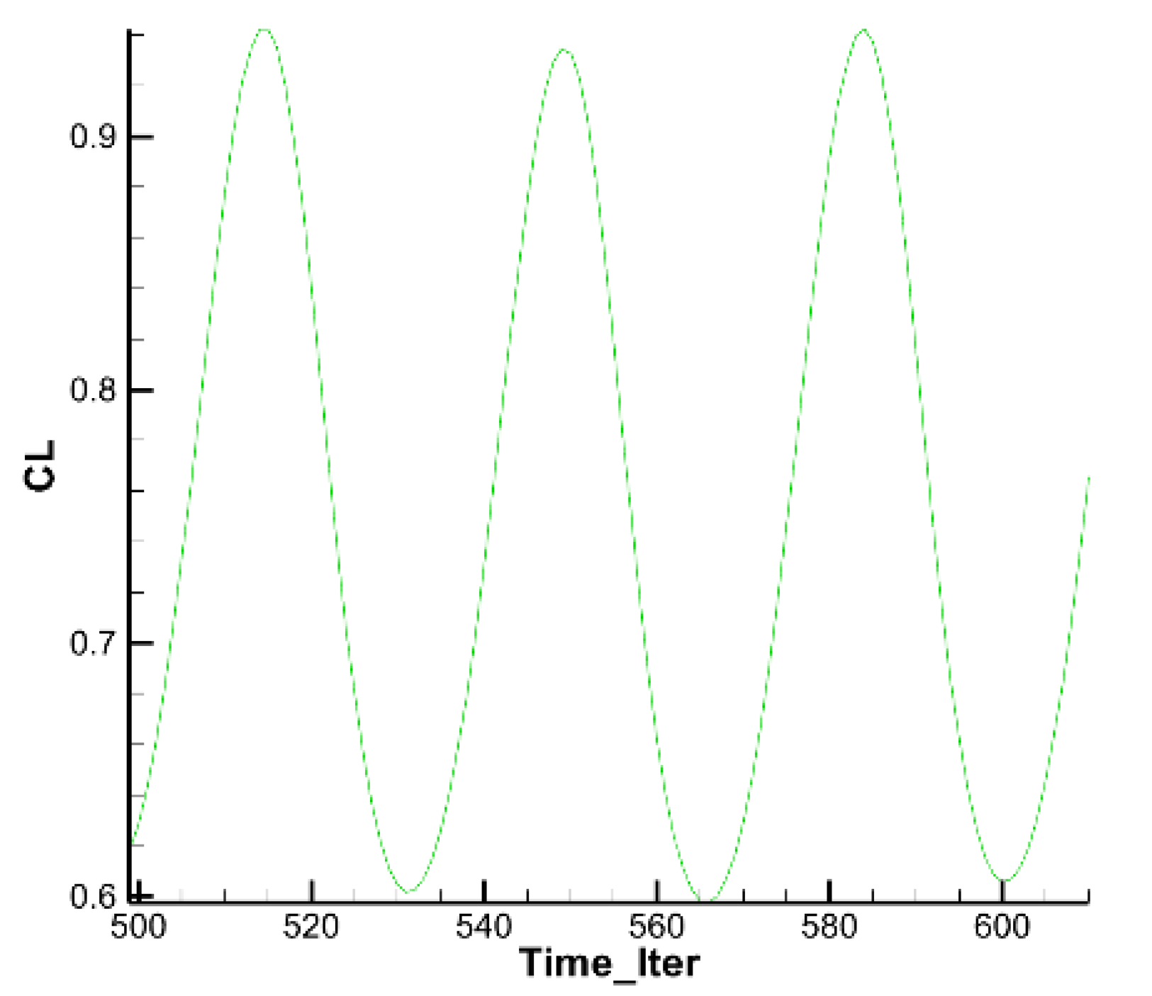
3. Airfoil Case Study

This study selects the two-dimensional NACA0012 airfoil provided by SU2 (version 7.0.1) as a case study for DMD analysis [23]. NACA0012 airfoil is widely used in fluid dynamics and aerodynamics research due to its simple geometric shape and complex flow characteristics, making it an ideal candidate for validating new methods and theories. The computation in this study utilized a mesh in SU2 format. The mesh consists of 14,576 nodes and 14,336 elements. The computational domain defines two boundary conditions: the airfoil surface and the farfield. The airfoil boundary is represented by 128 elements, while the farfield boundary is defined by 352 elements. The chord length of the airfoil model is 1 m, and the dimensions of the computational domain are approximately 1000 m in both the X and Y directions [24]. In this case, the flow conditions are set with a Mach number Ma = 0.3, Reynolds number Re = 1000.0 (set as a simplified parameter for computational purposes in SU2), and angle of attack α = 17.0°. The free-stream temperature is set at 293.0 K, and the free-stream pressure at 101325.0 Pa [25].

In the numerical computations, the Unsteady Reynolds-Averaged Navier–Stokes (URANS) method, based on RANS equations [26], is employed. The Spalart–Allmaras (SA) [27] turbulence model is used to simulate turbulent effects. A dual-time-stepping method is applied for time advancement, with a time step size of 5 × 10⁻⁴ s. A total of 112 snapshots are extracted, resulting in a snapshot matrix size of 14,576 × 112, where 14,576 corresponds to the spatial resolution (the number of grid points in the computational domain) and 112 represents the number of snapshots in the time series. Figure 1 illustrates the variation in the lift coefficient (C_L) with the number of iterations (Time_Iter) after the flow achieves stable unsteady periodic oscillations. The consistent amplitude and frequency of the oscillations indicate that the solution has reached a quasi-steady periodic state, demonstrating the convergence of the unsteady flow simulation.

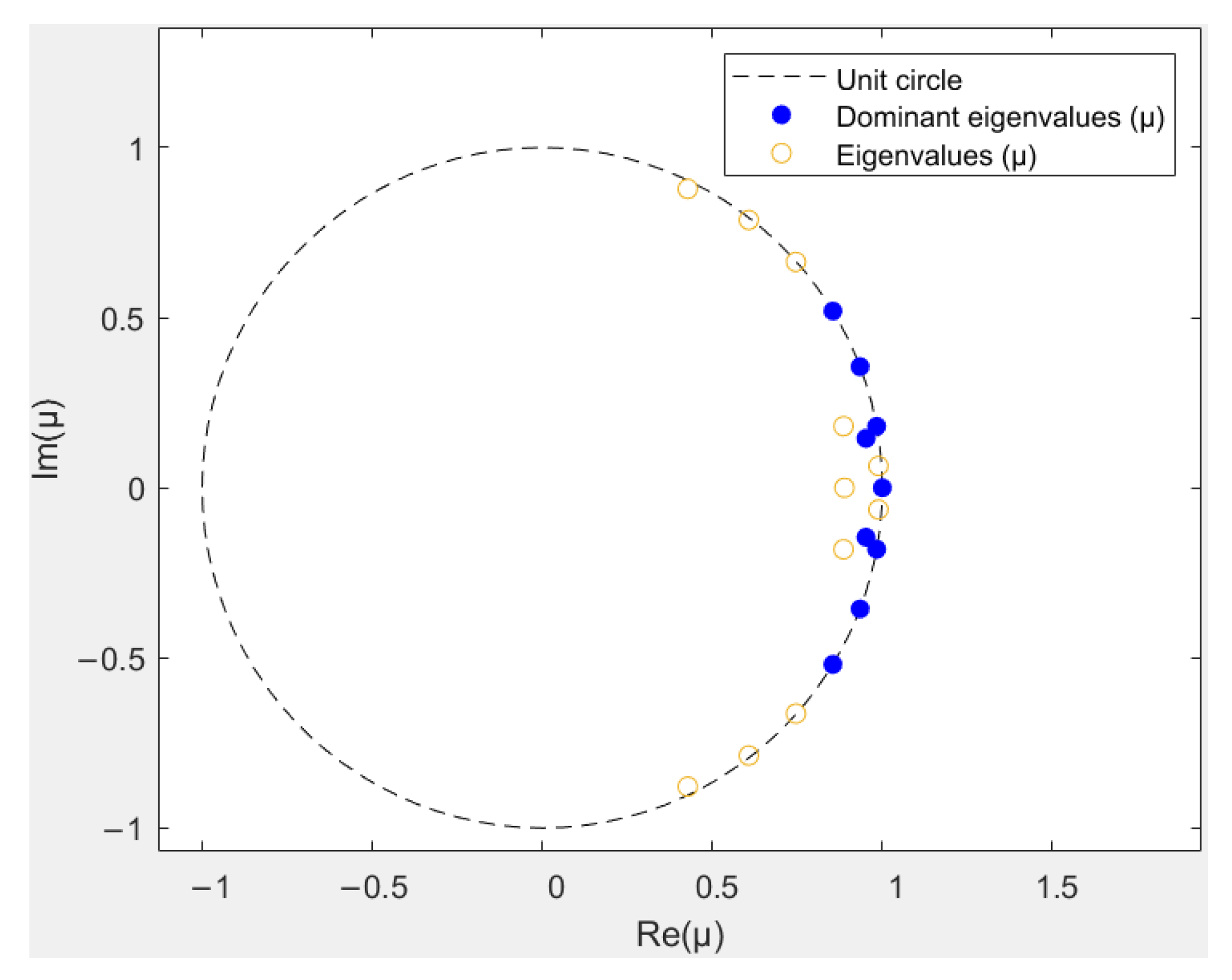
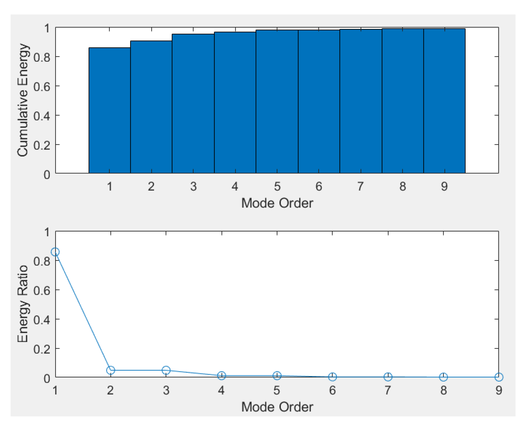
3.1. DMD Modal Analysis of Airfoil Case

The time snapshots are directly processed to construct a Mach number snapshot matrix, which is subsequently analyzed using DMD. In some studies, modes are ranked based on their modal amplitude [28]. However, to better reflect the energy contribution of each mode, this study combines the modal amplitude with the Frobenius norm for ranking [29]. A total of 20 DMD modes are computed, with special focus on the first mode and four pairs of conjugate modes. Since conjugate modes always appear in pairs, each pair is considered a single mode [30]. The first five modes are represented as solid blue circles.

As shown in Figure 2, the eigenvalues of the DMD modes are plotted on the complex plane. The eigenvalues of stationary modes lie on the unit circle, while the others are located near, but not exactly on, the unit circle. The eigenvalues on the unit circle represent periodic and neutrally stable modes whose amplitudes remain constant over time, reflecting the system’s primary periodic behavior. The eigenvalues inside of the unit circle correspond to decaying modes, whose amplitudes decrease over time, indicating stable behavior. Conversely, eigenvalues outside of the unit circle represent unstable modes, as their amplitudes grow with time.

To calculate the energy contribution of each mode, the following equation was used:

$$I_j=\sum _{i=1}^n\left|a_j\times {\lambda }_j^{i-1}\right|\times {{‖{\mathit{\varphi }}_{\mathit{j}}‖}_F}^2$$

(12)

where $a_j$ represents the modal amplitude, ${\lambda }_j$ denotes the modal eigenvalue, and ${‖{\mathit{\varphi }}_{\mathit{j}}‖}_F$ is the Frobenius norm of the modal vector. The energy contribution of each mode has been normalized as a ratio of the total energy.

The energy contribution of the first five modes is shown in Figure 3, demonstrating that the primary dynamic characteristics of the system are dominated by a few modes. The upper part of the two graphs displays the cumulative energy contribution, while the lower part illustrates the individual contribution of each mode. The results indicate that the first few modes account for the majority of the total energy, showing that the system’s primary behavior can be effectively captured by these modes. The first mode occupies a significant portion of the total energy, indicating that it captures the system’s core dynamic characteristics. As the mode order increases, the energy contribution of individual modes drops rapidly, suggesting that higher-order modes contain less information and have a limited impact on the overall dynamics.

Figure 4 shows the amplitude distribution of the DMD modes across different frequencies. The horizontal axis represents the frequency (f), while the vertical axis represents the amplitude (α), plotted on a logarithmic scale to better illustrate the data distribution. Since the modes are selected based on their energy contribution, they are not necessarily arranged in descending order of amplitude.

In DMD, the first mode typically represents the mean state of the system and is a static mode, with the highest amplitude and a frequency of 0. The growth rates and frequencies of the first five modes are listed in

Table 1. Growth rates and frequencies of dominant DMD modes.

DMD Mode	Growth Rate	Frequency/kHz
1	0	0
2	−0.2432	0.3633
3	−0.0049	0.7279
4	0.1672	1.0922
5	−75.599	0.3028

. As the first mode is static and analogous to a uniform flow field, both its growth rate and frequency are 0. The remaining four modes are conjugate modes, appearing in pairs.

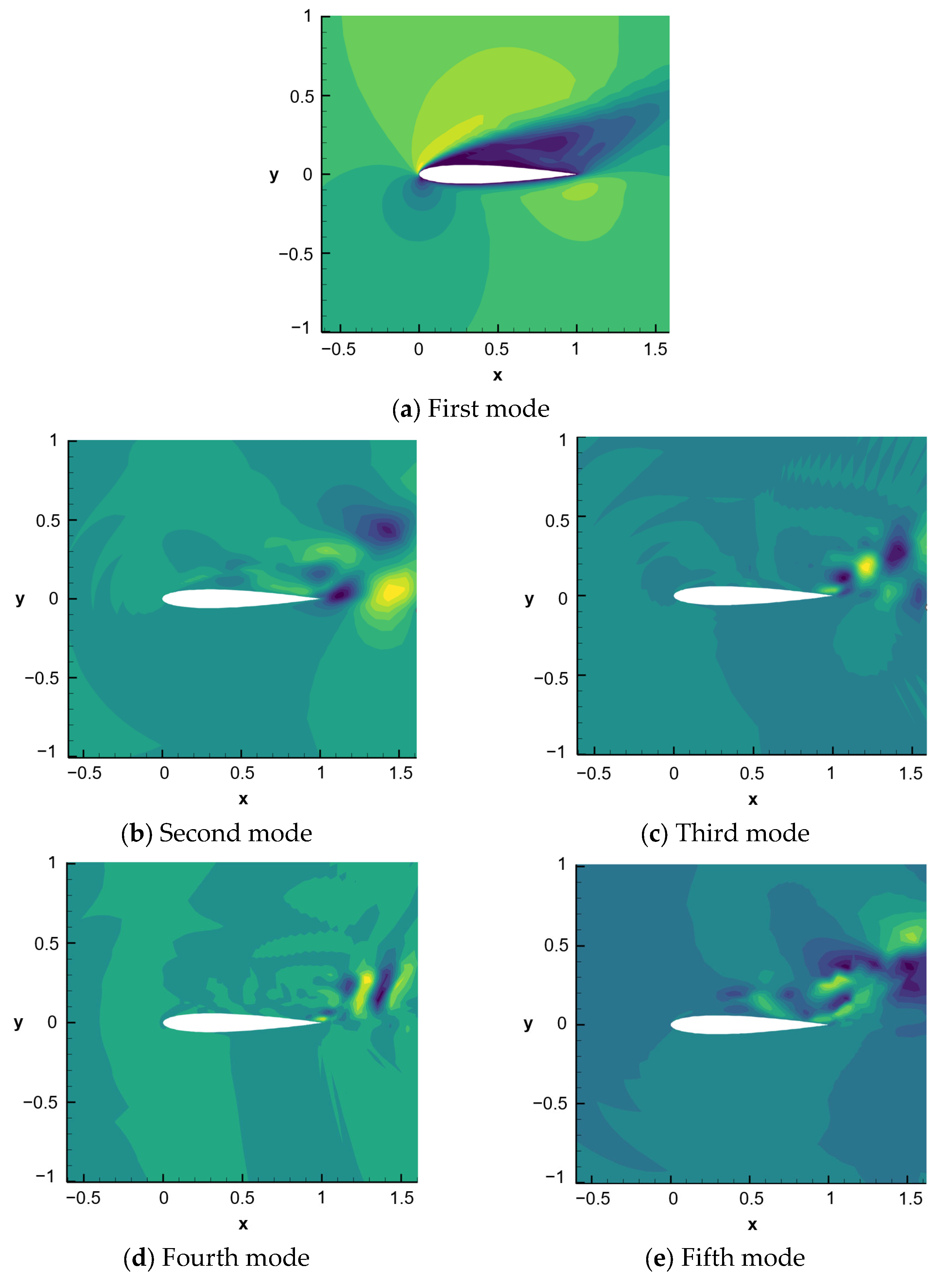
3.2. DMD Modal Contour Plot of Airfoil Case

The first five DMD modes with the highest energy are selected for processing, and the real part of the data contour plots obtained is shown in Figure 5. The first mode represents the mean characteristics of the flow field and the primary flow structure. The second and subsequent modes reveal instabilities and the presence of shedding vortex structures within the system. Through these modes, periodic variations and local instabilities in the flow can be observed, with unsteady phenomena mainly occurring in the wake region of the airfoil [31].

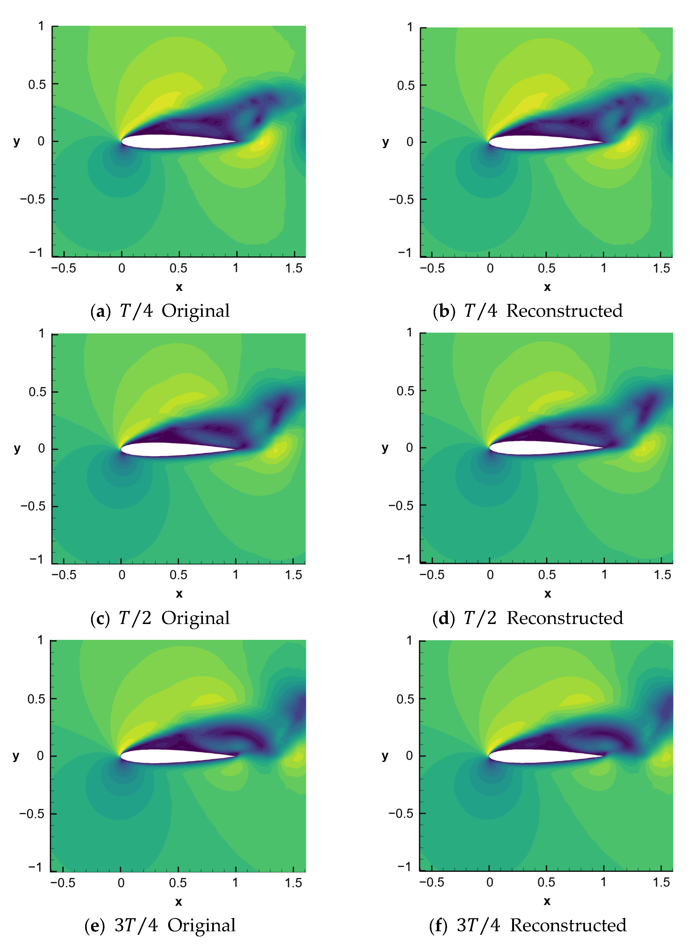
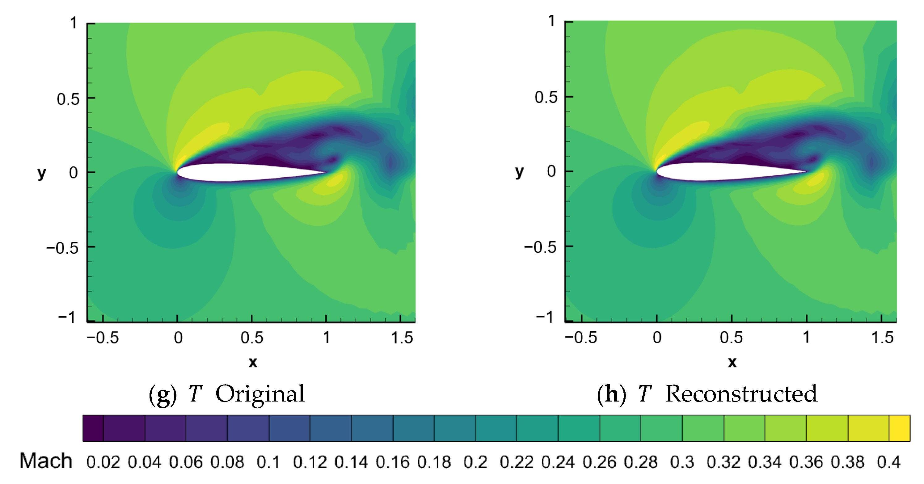
3.3. Reconstruction of Airfoil Case

The first five modes obtained through modal decomposition are used to reconstruct the flow field. The reconstruction process follows the following equation:

$$\tilde{X}(t)=\sum _{k=1}^n{a}_k{\mathit{\varphi }}_{\mathit{k}}{\lambda }_k^{t-1}$$

(13)

where $a_k$ represents the modal amplitude, ${\mathit{\varphi }}_{\mathit{k}}$ is the $k$-th mode, ${\lambda }_k$ is the eigenvalue associated with the mode, and $t$ denotes the time step.

A comparison of the Mach number between the reconstructed and original flow fields is shown in Figure 6, presenting the flow fields at four time instants within one period [32], as follows: T/4, T/2, 3T/4, and T. The comparison demonstrates that the reconstructed and original flow fields are almost identical, indicating that the reconstructed flow field accurately captures the structures within the flow. Combined with the previous energy distribution results, it can be concluded that the first five DMD modes contain sufficient information to represent the entire flow process effectively.

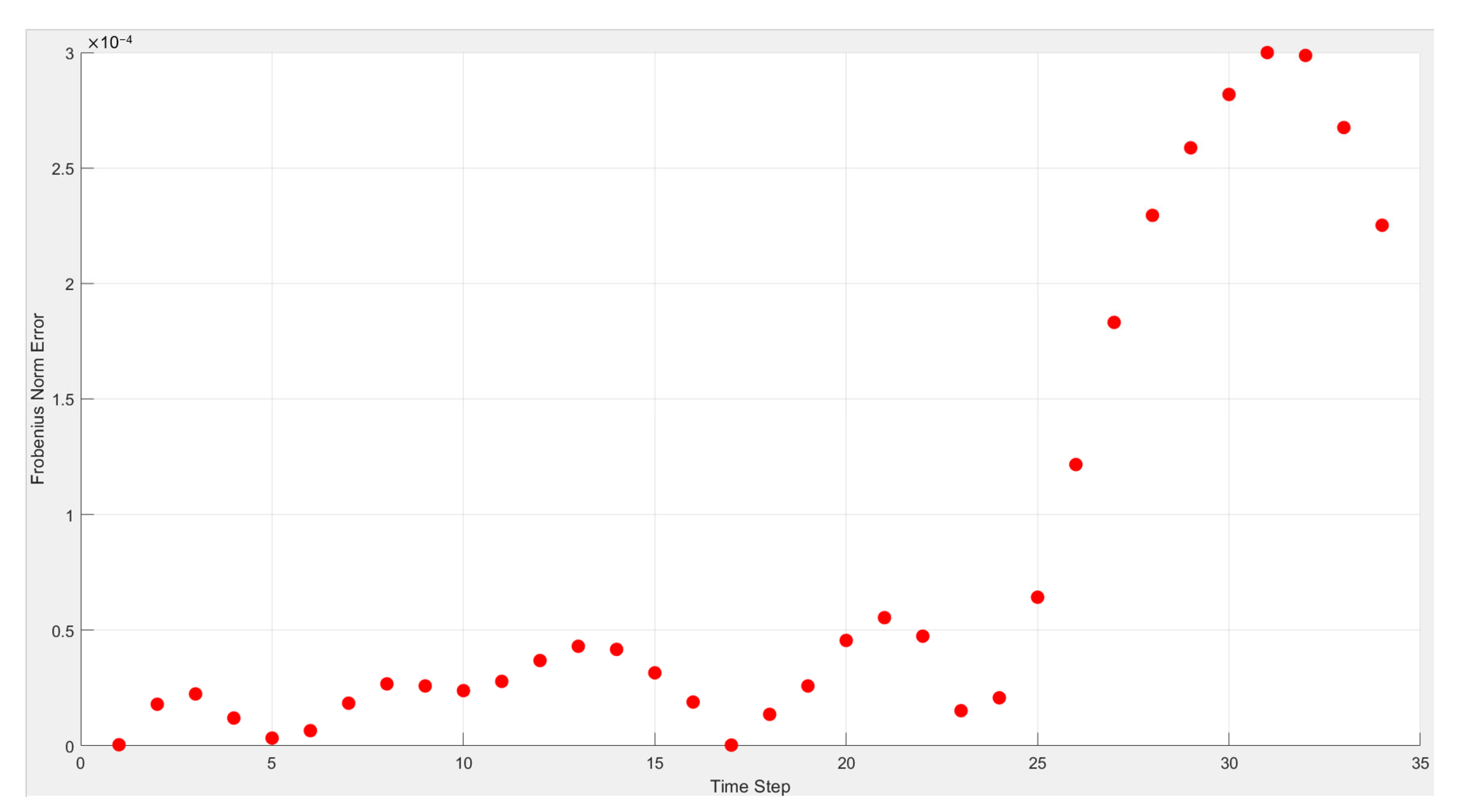
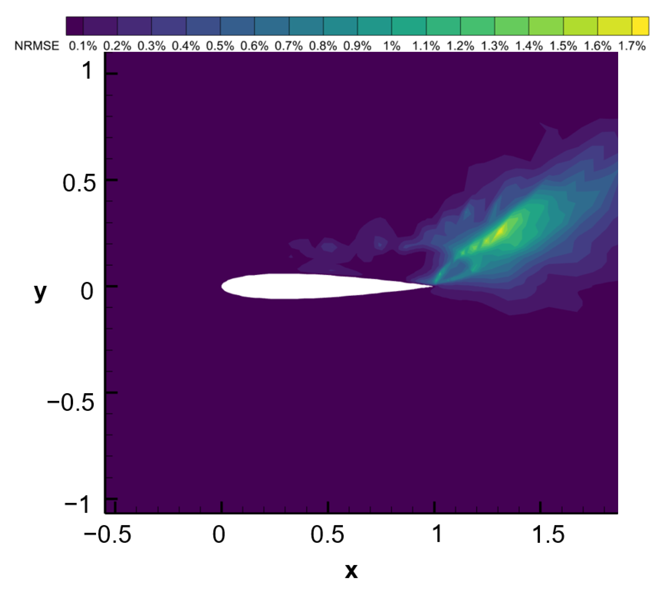
3.4. Error Analysis of Airfoil Case

To further validate the accuracy of DMD in reconstructing the unsteady flow field for this case study, we first conducted an error analysis on the reconstruction results over one complete period (34 time steps) of the simulation. The error is defined as the normalized difference between the Frobenius norm of the original pressure field and that of the DMD-reconstructed flow field. The specific calculation formula is as follows:

$$e\left(i\right)={\displaystyle \frac{\left|{‖M_i‖}_F-{‖D_i‖}_F\right|}{{‖M_i‖}_F}}$$

(14)

where ${‖M_i‖}_F$ represents the Frobenius norm of the original Mach number field at time step I, and ${‖D_i‖}_F$ denotes the Frobenius norm of the real part of the DMD-reconstructed Mach number field at the same time step. Figure 7 shows the relative error at each time step.

From the error plot, it can be clearly observed that the reconstruction error shows a significant increasing trend over time. In the first half of the period (approximately time steps 1 to 17), the error remains relatively small, staying below 5 × 10⁻⁵. However, in the later stages, the error increases rapidly, reaching its peak near the end of the period (around time steps 30 to 34), with a value close to 3 × 10⁻⁴. Although the error at each individual time step is relatively small, these errors can accumulate over time, especially in long-term reconstructions, where the effect becomes more pronounced. Due to modal truncation, only the modes with the highest energy contributions are retained, while the truncated modes, although contributing less energy, play a significant role in the long-term dynamic evolution of the system. In the reconstruction formula, time dependence is exponential, which further amplifies these errors over time. As the unsteady flow evolves, some dynamic behaviors in the system become more complex—such as vortex shedding and nonlinear oscillations, often associated with higher frequencies and finer flow structures—which contribute to the increase in error.

Overall, despite the slight increase in errors towards the end of the period, the error level remains low. The increase is mainly due to cumulative numerical errors and the growing complexity of the flow field. This indicates that the DMD method maintains a high level of reconstruction accuracy throughout the entire period, reliably capturing the primary dynamic behavior of the flow field.

However, the limitation of the Frobenius norm error lies in its ability to assess error only within individual time steps, making it difficult to capture the overall coupling of errors across different time steps throughout the entire period. As a result, it is challenging to comprehensively analyze the reconstruction accuracy from the perspective of the error distribution within the flow field structure. To address this limitation, we further introduce the root mean square error (RMSE) for a more comprehensive evaluation of the reconstruction error.

As an effective tool for measuring global error, the RMSE takes into account the accumulated errors across all time steps, reflecting the overall reconstruction error of the flow field throughout the entire period. With the RMSE, we can quantify the reconstruction error at each grid point over the entire time series and generate an error contour plot to visually display which regions have higher or lower errors. The specific calculation formula is as follows:

$${\epsilon }_{RMSE}\left(x_i\right)=\sqrt{{\displaystyle \frac{1}{T}}\sum _{t=1}^T{(M_{i,t}-D_{i,t})}^2}$$

(15)

where ${\epsilon }_{RMSE}\left(x_i\right)$ represents the cumulative root mean square error at grid point i; $M_{i,t}$ denotes the original Mach number value at grid point i and time step t; and $D_{i,t}$ represents the reconstructed Mach number value at the same grid point and time step. To better observe the relative error, the RMSE values are further normalized (NRMSE) by dividing them by the range (the difference between the maximum and minimum) of the original flow field data. Figure 8 shows the error contour plot after normalization.

Near the leading edge and surface of the airfoil, the DMD reconstruction error is relatively small, generally below 0.3%, indicating that the method can accurately capture the flow characteristics in these regions. However, at the trailing edge and wake regions, the NRMSE increases significantly, reaching approximately 1.5% in some areas. These regions exhibit complex flow behavior and are heavily influenced by unsteady vortex shedding and turbulence. This highlights the limitations of DMD in capturing the flow characteristics of highly nonlinear, turbulence-dominated flows, resulting in larger reconstruction errors in the wake region.

The normalized RMSE contour plot clearly illustrates the error distribution across different regions of the flow field. While the DMD method achieves high reconstruction accuracy in relatively stable regions, it shows certain limitations in areas with complex flow structures. These insights provide a valuable basis for the future optimization of reduced-order modeling for flow fields.

4. Compressor Cascade Analysis

In the calculations for this chapter, the URANS method is employed, along with the SST turbulence model [33] to simulate turbulent effects. The flow field is computed using unsteady simulations, with time advancement being achieved through a dual-time-stepping method [34]. The time step is set to 5 × 10⁻⁴ s, allowing the numerical solution of pressure and Mach number fields. Regarding the boundary conditions, the total pressure and static pressure are specified at the inlet and outlet, respectivley. The total inlet pressure is set to 101,400.0 Pa, with an inlet temperature of 288.0 K, and the outlet static pressure is 85,000 Pa. A mixed outlet averaging method is applied to manage the variations in pressure and Mach number during the computation. The Sutherland model [35] is used for the viscous effects, with appropriate reference viscosity and temperature settings. To ensure the accuracy of the numerical simulations, various numerical methods and solver parameters are utilized, including the weighted least-squares gradient calculation method, the ROE numerical scheme [36] for flows, and the Venkata limiter. Convergence is guaranteed by setting appropriate CFL numbers and configuring the linear solver parameters.

Figure 9 shows the variation in outlet mass flow rate with the number of iterations after the unsteady periodic oscillations reach a stable state.

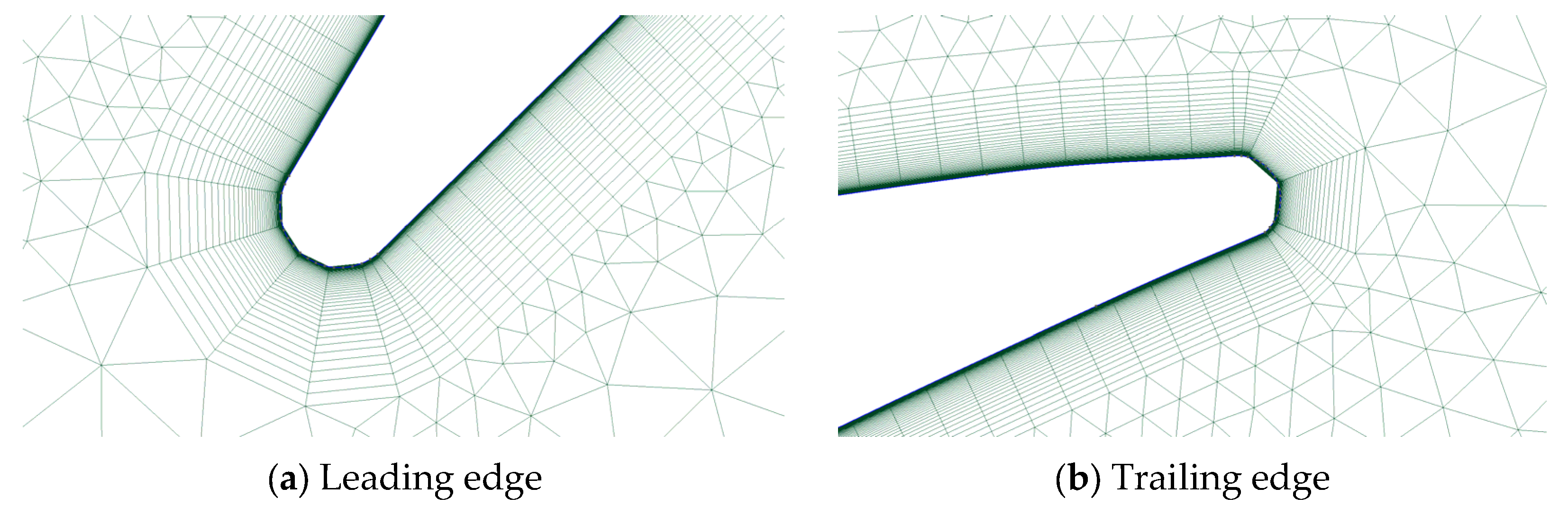
4.1. Research Object

In this chapter, the compressor cascade at a radial position of 100% (at the blade root) on the Stage35 compressor blade is selected as the research object for complete modeling, simulation, and DMD analysis. The model is first established based on the 2D parameters provided by NASA [37]. Some parameters of the blade are shown in

Table 2. Key parameters of compressor blade.

Inlet Angle	Outlet Angle	Chord	Solidity Rate	Setting Angle	Max Relative Thickness
51.69°	25.7°	5.622 cm	1.765	41.5°	0.458 cm

.

This study uses Gmsh software (version 4.10.4) for mesh generation. According to the flow characteristics of different regions, high-precision mesh division is performed on the Stage35 compressor cascade using a combination of structured and unstructured meshes. The mesh growth rate is set to 1.1, and prism elements are applied. The global control parameters are configured using the Frontal algorithm, with a random factor of 1 × 10⁻¹² and a geometric tolerance of 1 × 10⁻¹⁶. The final mesh model consists of 53,904 elements. The resulting snapshot matrix has a size of 50,650 × 1000. The overall mesh structure is shown in Figure 10, and the detailed mesh at the leading and trailing edges is shown in Figure 11.

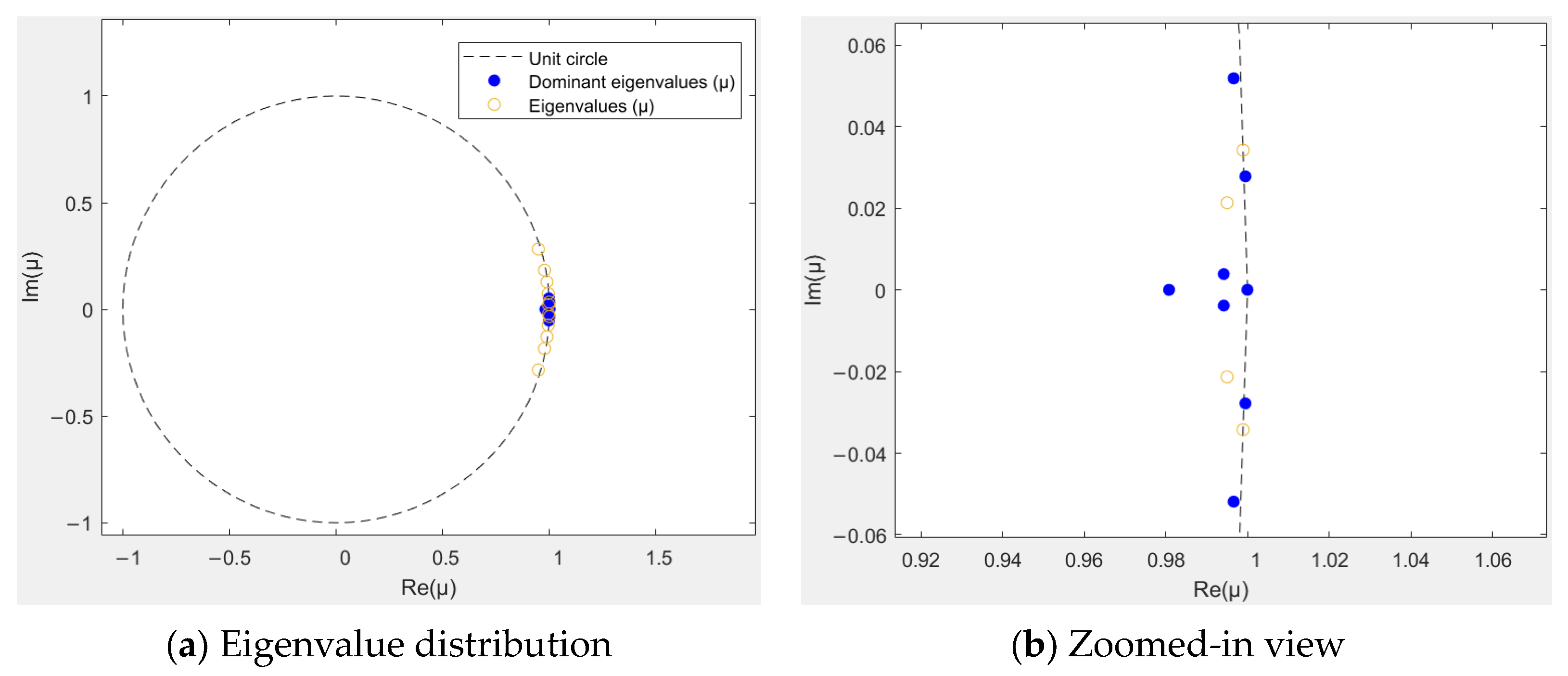
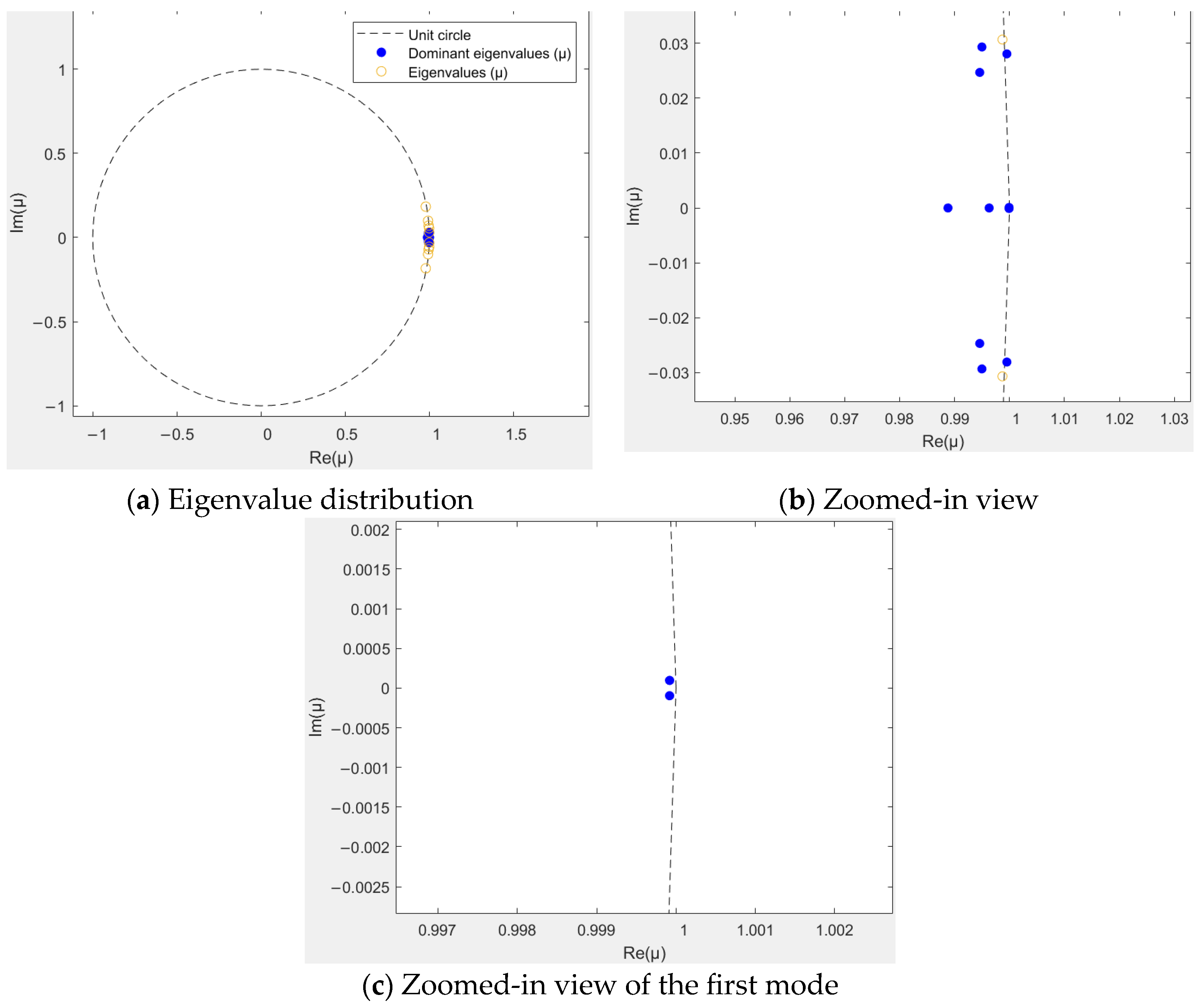
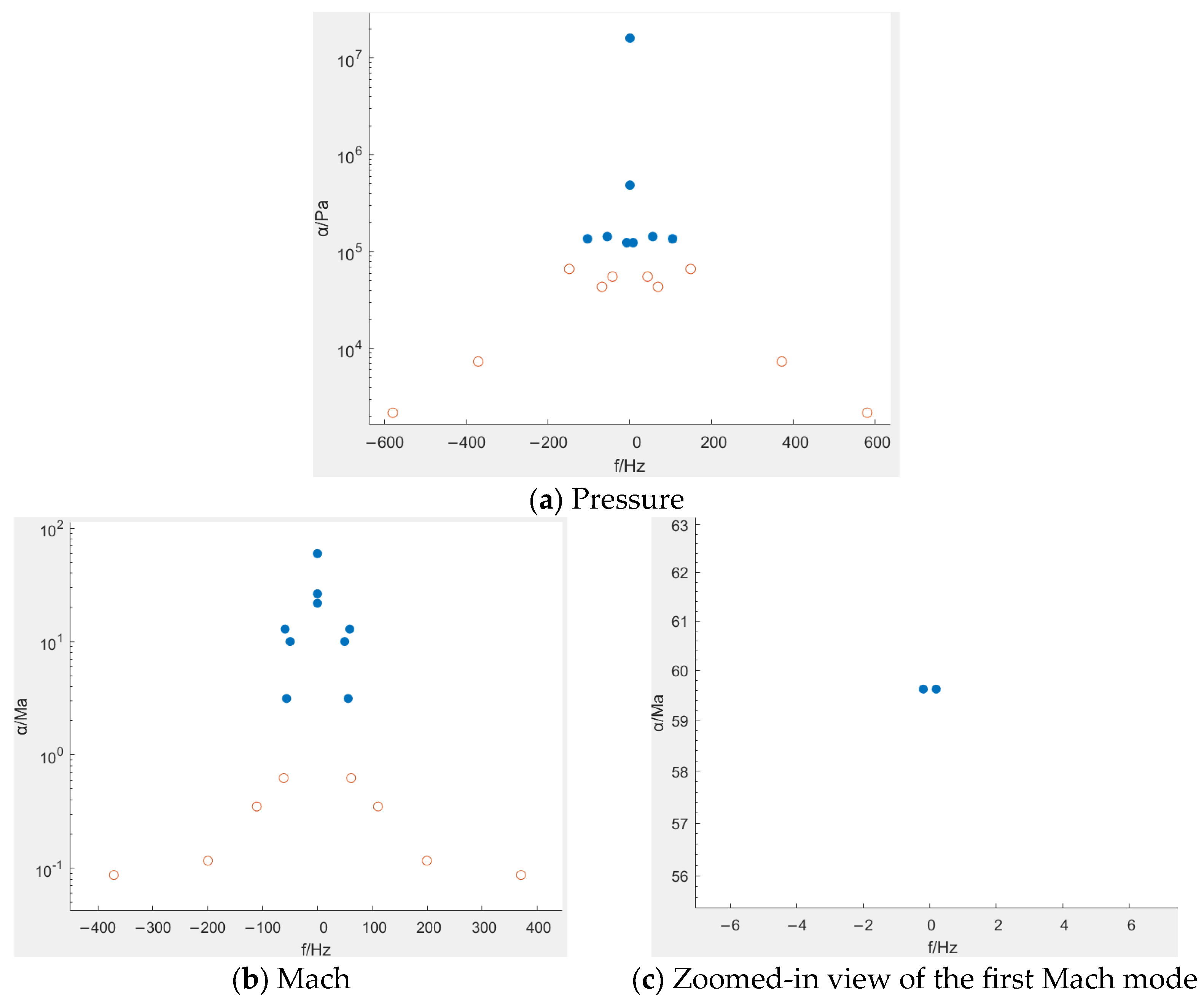
4.2. DMD Modal Analysis

Similar to the airfoil case study outlined in the previous chapter, a series of time snapshots obtained from the direct solution are processed to generate pressure snapshot matrices and Mach number snapshot matrices, which are then analyzed using DMD. The modes are ranked based on their energy contribution. A total of 20 DMD modes are calculated. For the pressure data, the focus is on the first mode, three pairs of conjugate modes, and one drift mode. These five modes are represented by solid blue circles in Figure 12. For the Mach number data, the focus is on the first mode, three pairs of conjugate modes, and two drift modes, represented by solid blue circles in Figure 13.

The drift modes reflect changes in the mean value of the flow field over time, and, therefore, have a frequency of 0 [20]. The modes with eigenvalues on the unit circle maintain a constant amplitude over time, reflecting the system’s primary periodic characteristics. On the other hand, the modes with eigenvalues inside of the unit circle represent decaying modes whose amplitudes gradually decrease over time, indicating energy loss or dissipation in the system. The farther the eigenvalues are from the unit circle, the faster the corresponding modes decay. Although these modes exist within the system, their influence is short-lived and has little impact on the system’s long-term behavior.

As shown in Figure 14, the energy distribution plot for the pressure data reveals that the first mode accounts for nearly 90% of the total energy, indicating that the primary dynamic behavior of the pressure data is almost entirely governed by the first mode, with the remaining modes contributing very little energy. In the energy distribution plot for the Mach number data, the first and second modes capture the majority of the total energy. Although their proportion is significantly lower than that observed in the pressure data, they still play a dominant role. The energy contribution plot for each mode reveals that, beyond the first and second modes, the energy of the remaining modes decays rapidly. The cumulative energy of these displayed modes accounts for 97% of the total energy. This suggests that, for both the pressure data and Mach number data, the primary dynamic characteristics of the system are dominated by the first few modes, with the remaining modes having minimal impact on the system’s dynamic behavior.

Figure 15 shows the amplitude distribution of DMD modes across different frequencies, with the horizontal axis representing frequency (f) and the vertical axis representing amplitude (α), using a logarithmic scale to better display the data distribution. According to

Table 3. Growth rates and frequencies of dominant DMD modes.

DMD Mode	Growth Rate (Pressure)	Frequency/kHz (Pressure)	Growth Rate (Mach)	Frequency/kHz (Mach)
1	0	0	−0.1618	0.0002
2	−11.618	0.0078	−7.4182	0
3	−38.836	0	−22.530	0
4	−0.2379	0.0557	−9.2040	0.0589
5	−4.0631	0.1040	−10.251	0.0496
6	——	——	−0.1782	0.0561

, for the pressure data, the first mode represents the system’s average state, which is a static mode and is similar to a uniform flow field. Therefore, it has the largest amplitude, with both the growth rate and the frequency being 0. In contrast, for the Mach number data, the first mode is composed of a pair of conjugate modes, indicating the presence of periodic oscillations in the Mach number field. This suggests that the Mach number flow system is governed by low-frequency oscillation modes, rather than steady-state flow. The first DMD mode of the pressure data represents the average flow field, while the first DMD mode of the Mach number data is composed of conjugate modes, illustrating the differences in the dominant dynamic characteristics of different physical quantities within the flow system [38].

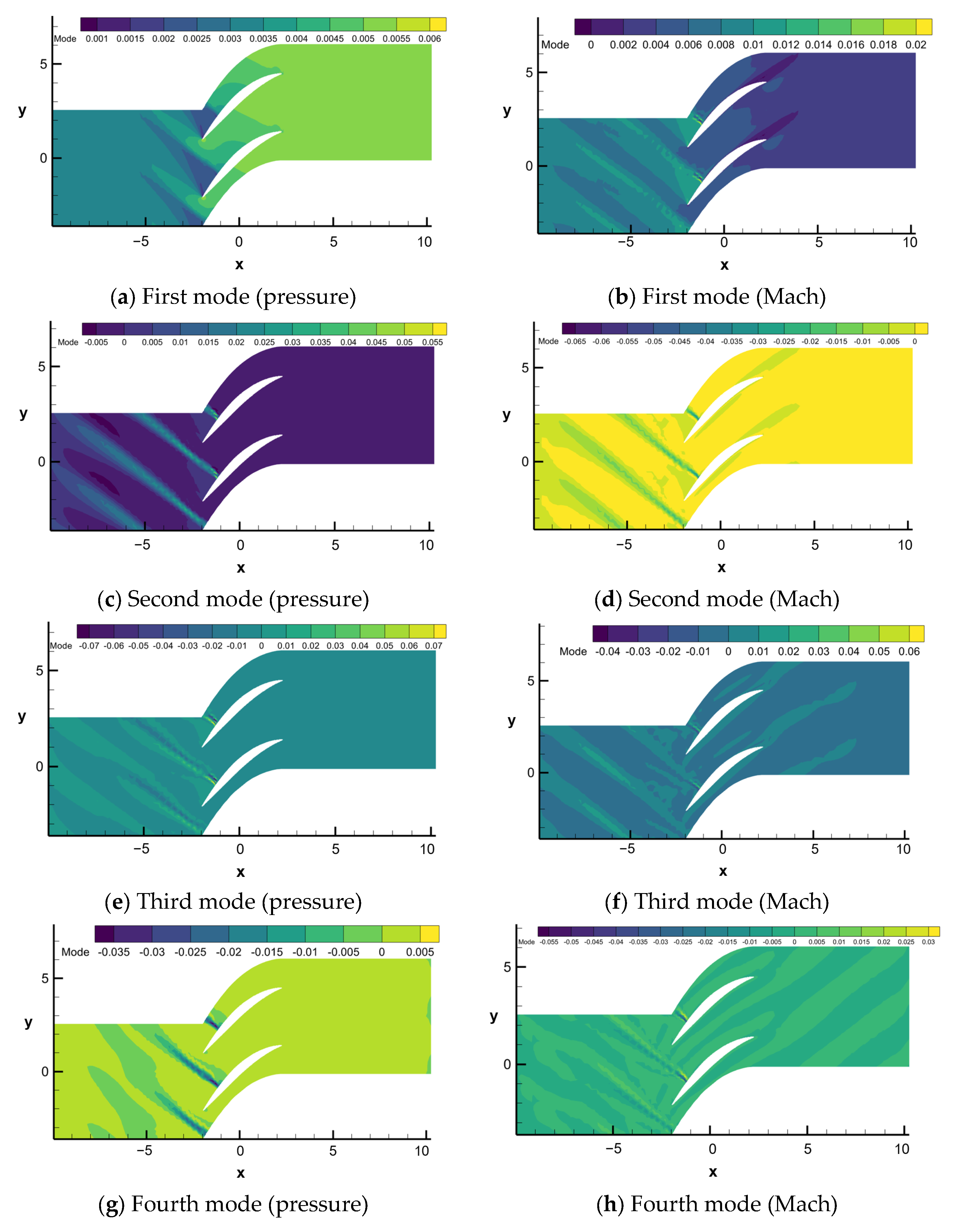
4.3. DMD Modal Contour Plot

The first five DMD modes are selected for processing, and the real part of the data contour plots is shown in Figure 16. The first mode of the pressure data represents the average characteristics of the flow field and the primary flow structure. Meanwhile, the first mode of the Mach number data, despite being a pair of conjugate modes, has an extremely low frequency, close to 0. This low-frequency oscillation mode contour plot is somewhat similar to steady-state average flow. Each mode exhibits significant numerical variations at the shock wave discontinuities, indicating that these modes can, to some extent, reflect the periodic changes of the shock waves [39].

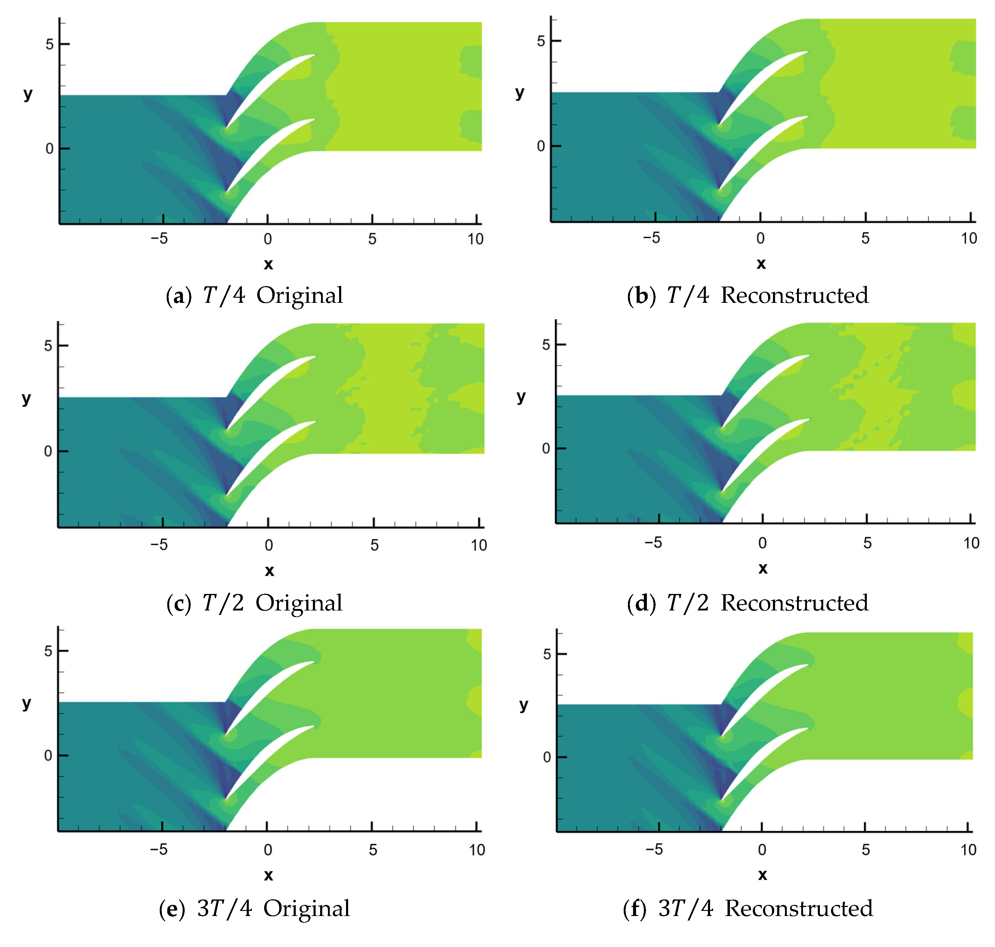
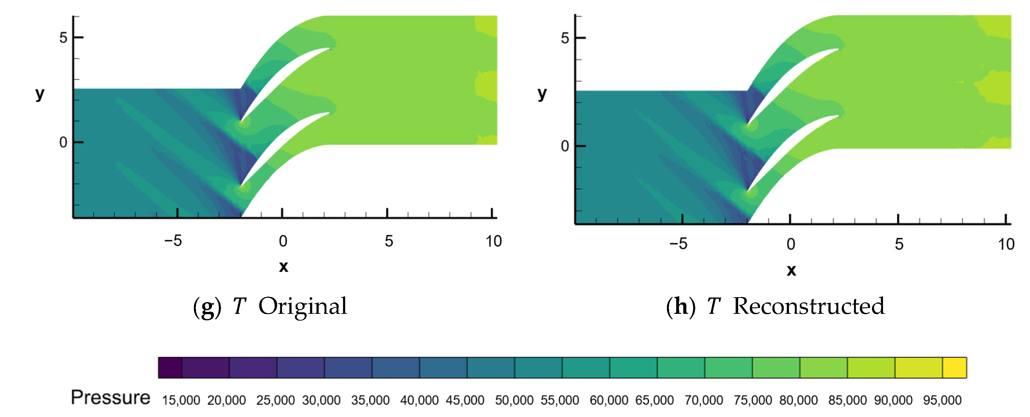
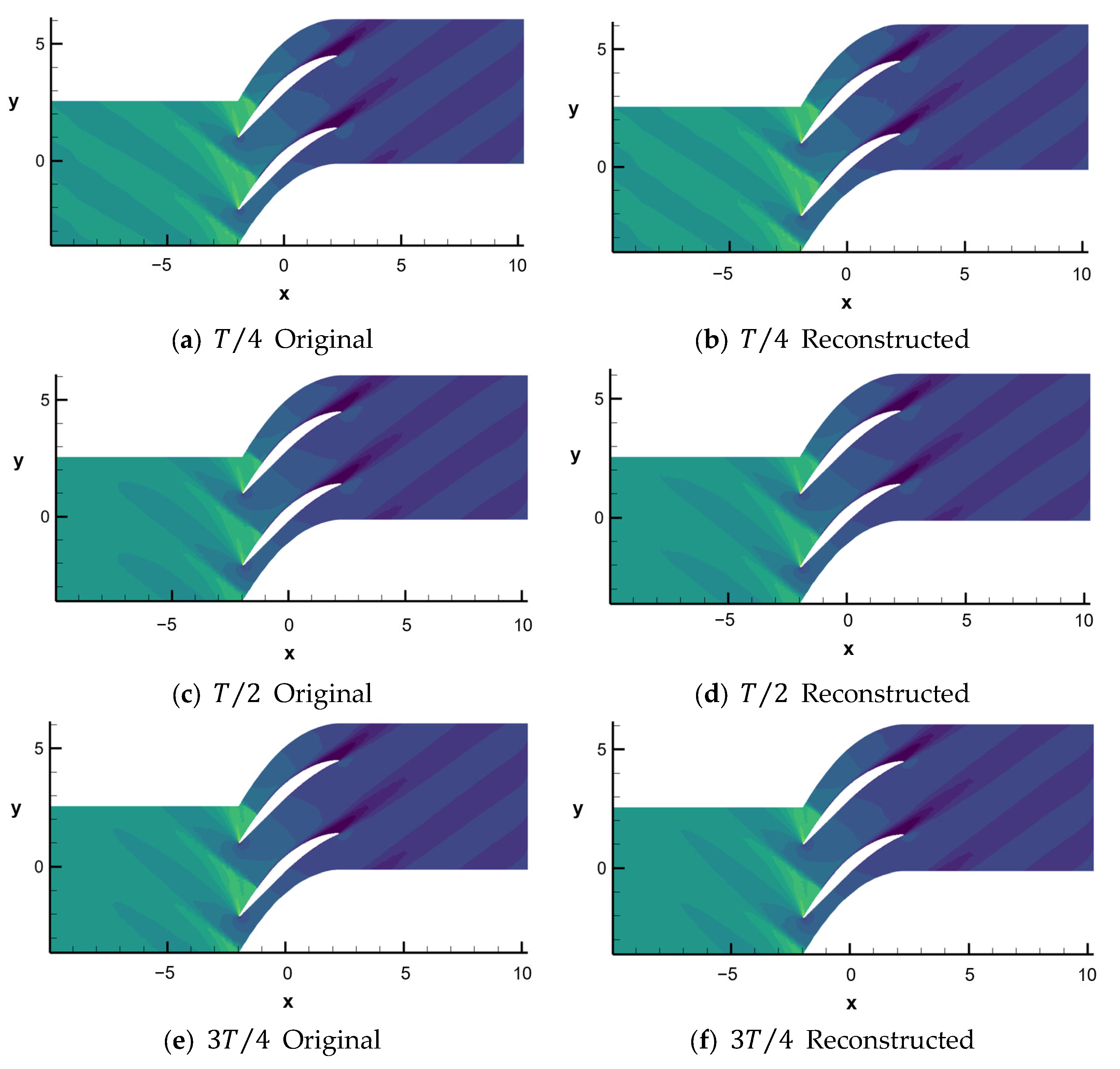
4.4. Reconstruction

The flow field is reconstructed using the first five pressure modes and the first ten Mach modes obtained through modal decomposition. The pressure and Mach number comparisons are shown in Figure 17 and Figure 18, presenting the reconstructed and original flow fields at four time instants—T/4, T/2, 3T/4, and T—within one period. The comparison shows that the contour structure distributions of both are almost identical, indicating that the reconstructed flow field accurately describes the various structures within the flow. Combined with the previous energy distribution results, it can be concluded that the DMD modes studied here contain sufficient information to effectively represent the entire flow process.

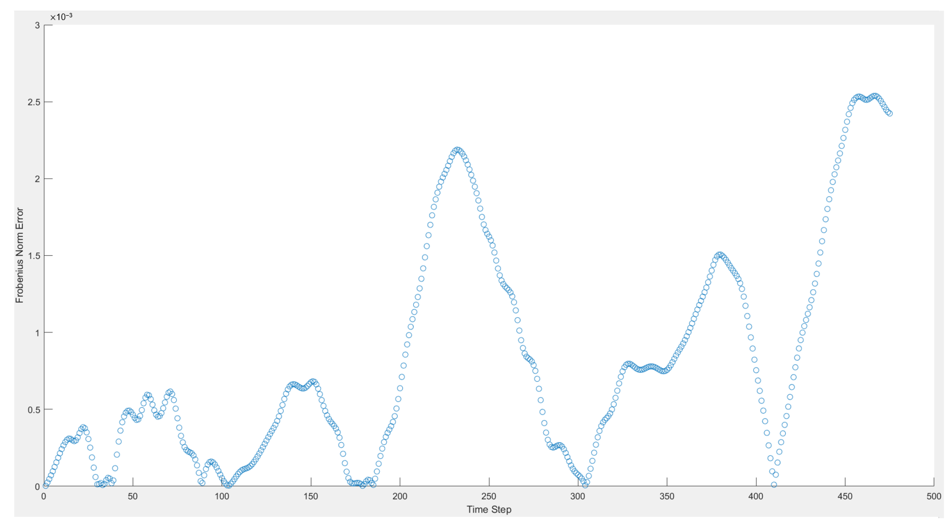
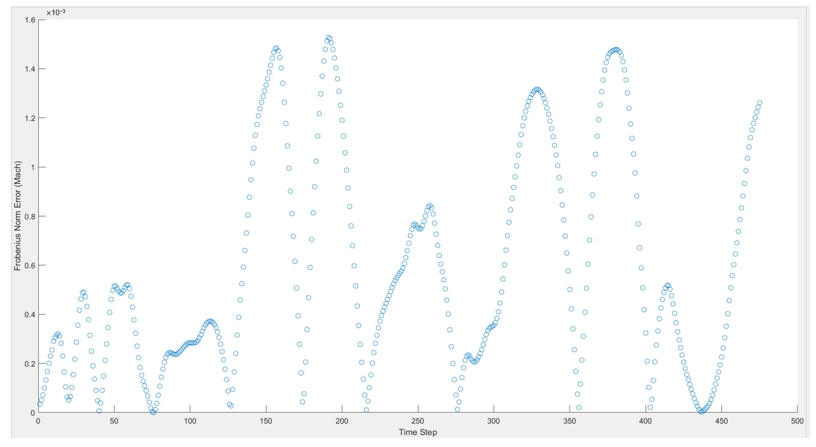
4.5. Error Analysis

Similar to the previous chapter, an error analysis is performed on the reconstructed flow field of the compressor cascade over one period. The Frobenius norm error is shown in Figure 19 and Figure 20.

The relative error distribution curve of the pressure data shows a certain periodic fluctuation. In the first half (approximately time steps 1 to 200), the error remains relatively small and stable, staying mostly below 5 × 10⁻⁵. However, the error gradually increases in the latter half of the period, especially near the end, with the error reaching a maximum close to 2.5 × 10⁻⁴ at around time step 400. The relative error distribution of the Mach number data is similar to that of the pressure data, also exhibiting periodic fluctuations. However, the Mach number data show larger fluctuations earlier on, with higher peak errors. This difference may be related to the turbulence characteristics in the Mach number field and the influence of shock wave structures on the flow field. The Mach number is more sensitive to high-speed variation regions in the flow field, such as vortex shedding and other unsteady phenomena. Throughout the period, although the error fluctuates, the reconstruction error remains at a relatively low level and shows a periodic growth trend. This trend aligns with the evolution of unsteady dynamic behaviors in the flow field.

The RMSE after normalization is shown in Figure 21. The pressure data reconstruction error plot shows that most regions of the cascade structure have relatively low errors, with NRMSE values mostly below 1%. However, a diagonal high-error zone forms within the blade passages, with the highest NRMSE being around 9.5%. The Mach number reconstruction error plot exhibits a similar spatial distribution, but the overall error level is lower, with NRMSE values being below 0.5% in most regions. A diagonal high-error zone also forms in the blade passages, with the maximum NRMSE being around 6.5%. The error in most areas of the reconstructed flow field remains low, reflecting the accuracy of DMD in capturing the flow characteristics. However, near the shock wave discontinuities, where the flow is more complex, the ability of DMD to capture these characteristics is insufficient, leading to relatively larger errors. Future research can focus on optimizing the DMD reconstruction capability for these complex flow regions.

5. Conclusions

In this paper, the flow fields of the NACA0012 airfoil case and the Stage35 compressor cascade were analyzed using the standard DMD method, leading to the following conclusions:

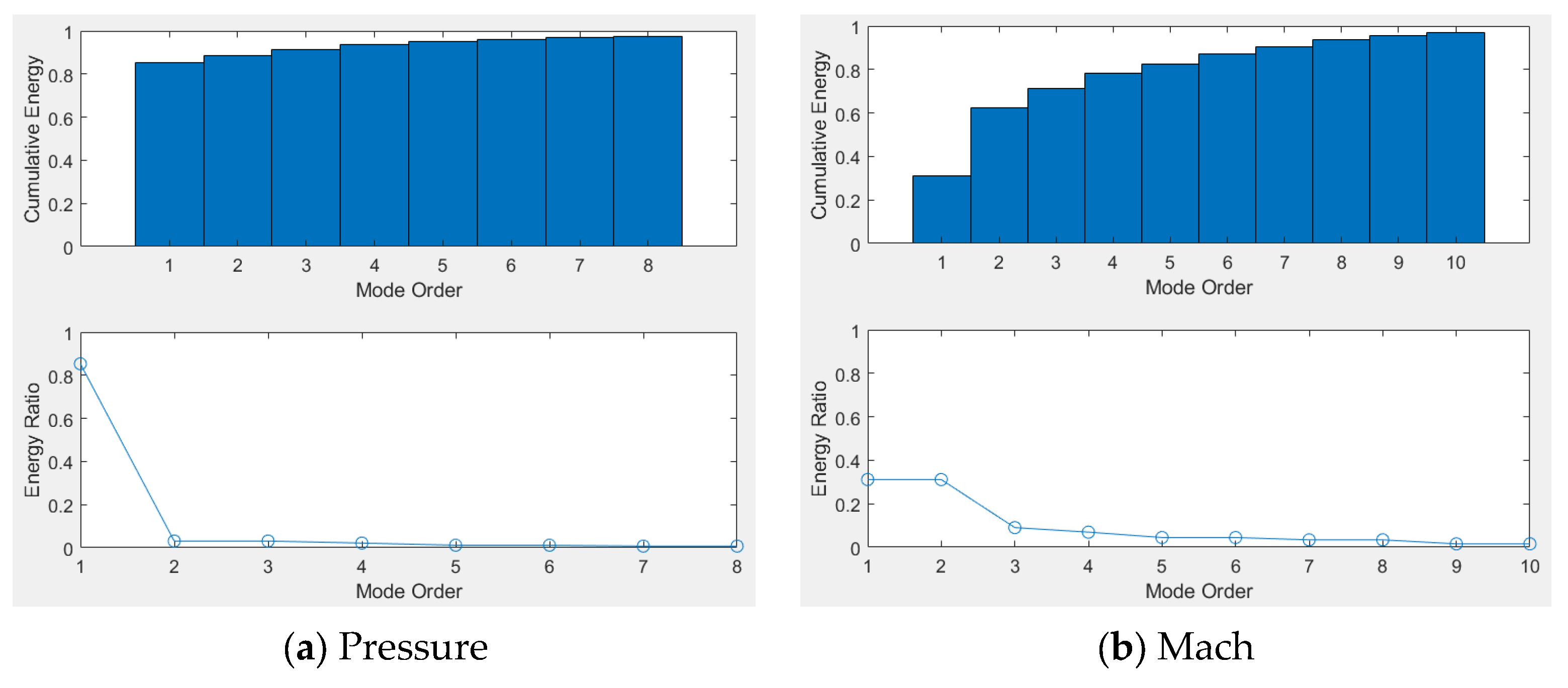
• The DMD analysis of the unsteady flow field of the Stage35 compressor cascade verified the effectiveness of the DMD method in addressing complex flow problems. The results show that the first six modes captured the majority of the system’s energy, effectively capturing the primary dynamic behavior of the flow field;
• Using the dominant DMD modes obtained from the decomposition, the flow field was reconstructed. The contour plots generated from the reconstructed data for both the pressure field and the Mach number field closely match the original flow field, indicating that the DMD modes can accurately reproduce the primary structures in the flow field;
• Through error analysis, we found that the overall reconstruction error when using DMD was relatively low, with higher errors only occurring in regions with complex flow structures. Future work can focus on optimizing the DMD method to improve the reconstruction accuracy in these regions.

However, in practical applications, due to the high dimensionality of the data, large sample sizes, and the presence of noise and errors, the standard DMD method still faces many challenges. To address these issues, researchers have proposed various improved DMD algorithms, such as Optimal Mode Decomposition [40], Sparsity-Promoting DMD [41], Multi-Resolution DMD [42], DMD with Control [43], Total DMD [44], and Streaming DMD [45]. With these improvements, future applications and research on DMD will become more extensive and in-depth.

References

- Zhang, L.; Deng, X.; He, L.; Li, M.; He, X. The opportunity and grand challenges in computational fluid dynamics by exascale computing. Acta Aerodyn. Sin. 2016, 34, 405–417. [Google Scholar] [CrossRef]
- Pearson, K.L., III. On lines and planes of closest fit to systems of points in space. Lond. Edinb. Dublin Philos. Mag. J. Sci. 1901, 2, 559–572. [Google Scholar] [CrossRef]
- Hotelling, H. Analysis of a complex of statistical variables into principal components. J. Educ. Psychol. 1933, 24, 417. [Google Scholar] [CrossRef]
- Lu, K.; Jin, Y.; Chen, Y.; Yang, Y.; Hou, L.; Zhang, Z.; Li, Z.; Fu, C. Review for order reduction based on proper orthogonal decomposition and outlooks of applications in mechanical systems. Mech. Syst. Signal Process. 2019, 123, 264–297. [Google Scholar] [CrossRef]
- Fogleman, M.; Lumley, J.; Rempfer, D.; Haworth, D. Application of the proper orthogonal decomposition to datasets of internal combustion engine flows. J. Turbul. 2004, 5, 023. [Google Scholar] [CrossRef]
- Zhu, J.; Huang, G.; Fu, X. Spatiotemporal characteristics analysis for controlling flow separation in divergent curved channels with POD method. Acta Aeronaut. Astronaut. Sin. 2014, 35, 921–932. [Google Scholar] [CrossRef]
- Dong, S.; Shi, A.; Ye, Z.; Tian, H. CFD computation and POD analysis for transonic buffet on a supercritical airfoil. Acta Aerodyn. Sin. 2015, 33, 481–487. [Google Scholar] [CrossRef]
- Hall, K.C.; Thomas, J.P.; Dowell, E.H. Proper orthogonal decomposition technique for transonic unsteady aerodynamic flows. AIAA J. 2000, 38, 1853–1862. [Google Scholar] [CrossRef]
- Chen, L.; Xu, C.; Lu, X. Numerical investigation of the compressible flow past an aerofoil. J. Fluid Mech. 2010, 643, 97–126. [Google Scholar] [CrossRef]
- Yu, H.; Chen, Y. Application of POD method to reduce dimensions of rotor system. J. Harbin Univ. Commer. Nat. Sci. Ed. 2012, 28, 365–368. [Google Scholar] [CrossRef]
- Chen, K.; Zhang, Y.; Lei, Y.; Lu, A.; Zhang, D. Wake analysis of pulsed jet based on proper orthogonal decomposition. Chin. J. Appl. Mech. 2022, 39, 834–844. [Google Scholar] [CrossRef]
- Zhang, Y.; Wang, Z.; Qiu, R.; Xi, G. Improved POD-Galerkin reduced order model with long short-term memory neural network and its application in flow field prediction. J. Xi’an Jiaotong Univ. 2024, 58, 12–21. [Google Scholar] [CrossRef]
- Kou, J. Reduced-Order Modeling Methods for Unsteady Aerodynamics and Fluid Flows. Master’s Thesis, Northwestern Polytechnical University, Xi’an, China, 2018. [Google Scholar] [CrossRef]
- Schmid, P.J. Dynamic mode decomposition of numerical and experimental data. J. Fluid Mech. 2010, 656, 5–28. [Google Scholar] [CrossRef]
- Tissot, G.; Cordier, L.; Benard, N.; Noack, B.R. Model reduction using dynamic mode decomposition. Comptes Rendus. Mécanique 2014, 342, 410–416. [Google Scholar] [CrossRef]
- Barocio, E.; Pal, B.C.; Thornhill, N.F.; Messina, A.R. A dynamic mode decomposition framework for global power system oscillation analysis. IEEE Trans. Power Syst. 2014, 30, 2902–2912. [Google Scholar] [CrossRef]
- Al-Jiboory, A.K. Adaptive quadrotor control using online dynamic mode decomposition. Eur. J. Control 2024, 80, 101117. [Google Scholar] [CrossRef]
- Zhu, J.; Zhou, X.; Kikumoto, H. Source term estimation in the unsteady flow with dynamic mode decomposition. Sustain. Cities Soc. 2024, 115, 105843. [Google Scholar] [CrossRef]
- Santana, G.; Fabro, A.; Miserda, R. Analysis of the dynamic modes of the transonic flow around a cylinder. J. Braz. Soc. Mech. Sci. Eng. 2024, 46, 581. [Google Scholar] [CrossRef]
- Li, Z.; Zhou, J.; Zhu, X.; Zhou, J.; Pan, T. Investigation of Reynolds number effects on flow stability of a transonic compressor using a dynamic mode decomposition method. Aerosp. Sci. Technol. 2024, 153, 109421. [Google Scholar] [CrossRef]
- Gilotte, P.; Mortazavi, I.; Edwige, S. Active control and modal decomposition for the flow over a ramp. Int. J. Heat Fluid Flow 2024, 107, 109374. [Google Scholar] [CrossRef]
- Schmid, P.J. Application of the dynamic mode decomposition to experimental data. Exp. Fluids 2011, 50, 1123–1130. [Google Scholar] [CrossRef]
- SU2 Tutorials. Available online: https://github.com/su2code/Tutorials/tree/master/compressible_flow/Unsteady_NACA0012 (accessed on 20 June 2024).
- Aasha, G.C.; Raj, V.; Kolluru, R.; Chalkapure, R.M.; Srikanth, R.; Ajit, H.A. Numerical Simulation of Flow over NACA-0012 Airfoil Pitching at Low Frequencies. In Proceedings of the SU2 Conference 2020, Bengaluru, India, 10–12 June 2020. [Google Scholar]
- Kurtulus, D.F. Aerodynamic Loads of Small-Amplitude Pitching NACA 0012 Airfoil at Reynolds Number of 1000. AIAA J. 2018, 56, 3328–3331. [Google Scholar] [CrossRef]
- Reynolds, O. XXIX. An Experimental Investigation of the Circumstances Which Determine Whether the Motion of Water Shall Be Direct or Sinuous, and of the Law of Resistance in Parallel Channels. Philos. Trans. R. Soc. Lond. 1883, 174, 935–982. [Google Scholar] [CrossRef]
- Spalart, P.; Allmaras, S. A One-Equation Turbulence Model for Aerodynamic Flows. Aerosp. Sci. Meet. 1992, 30, 439. [Google Scholar] [CrossRef]
- Hu, W.; Yu, J.; Liu, H.; Yan, C. Dynamic modal analysis of circular-arc airfoil transonic flow. J. Beijing Univ. Aeronaut. Astronaut. 2019, 45, 1026–1032. [Google Scholar] [CrossRef]
- Kou, J.; Zhang, W. An improved criterion to select dominant modes from dynamic mode decomposition. Eur. J. Mech. -B/Fluids 2017, 62, 109–129. [Google Scholar] [CrossRef]
- Kou, J.; Zhang, W. Dynamic mode decomposition and its applications in fluid dynamics. Acta Aerodyn. Sin. 2018, 36, 163–179. [Google Scholar] [CrossRef]
- Hu, S.; Chen, B.Z.; Kang, W. Lift improvement and mechanism study of membrane airfoil using dynamic mode decomposition. Acta Aeronaut. Astronaut. Sin. 2021, 42, 61–72. [Google Scholar] [CrossRef]
- Liu, P.Y.; Chen, J.G.; Shen, X. Dynamic mode decomposition analysis of wind turbine airfoil in high angle flowfield. J. Shanghai Jiao Tong Univ. 2017, 51, 805–811. [Google Scholar] [CrossRef]
- Menter, F.R. Two-Equation Eddy-Viscosity Turbulence Models for Engineering Applications. AIAA J. 1994, 32, 1598–1605. [Google Scholar] [CrossRef]
- Jameson, A. Time Dependent Calculations Using Multigrid, with Applications to Unsteady Flows Past Airfoils and Wings. In Proceedings of the 10th Computational Fluid Dynamics Conference, Honolulu, HI, USA, 24–26 June 1991; p. 1596. [Google Scholar] [CrossRef]
- Sutherland, W. The Viscosity of Gases and Molecular Force. Lond. Edinb. Dublin Philos. Mag. J. Sci. 1893, 36, 507–531. [Google Scholar] [CrossRef]
- Roe, P.L. Approximate Riemann Solvers, Parameter Vectors, and Difference Schemes. J. Comput. Phys. 1981, 43, 357–372. [Google Scholar] [CrossRef]
- Messenger, H.E.; Kennedy, E.E. Two-Stage Fan I: Aerodynamic and Mechanical Design; NASA Contractor Report, NASA CR-120859; Glenn Research Center: Cleveland, OH, USA, 1972. [Google Scholar]
- Hu, J.; Wang, Y.; Liu, H. Comparative Study on Modal Decomposition Methods of Unsteady Separated Flow in Compressor Cascade. J. Northwestern Polytech. Univ. 2020, 38, 121–129. [Google Scholar] [CrossRef]
- Wang, J.; Liu, X.D.; Xia, J.Z. Flow field reconstruction and characteristic analysis of dual-throat control vector nozzle based on dynamic mode decomposition. Acta Aeronaut. Astronaut. Sin. 2024, 39, 191–200. [Google Scholar] [CrossRef]
- Wynn, A.; Pearson, D.S.; Ganapathisubramani, B.; Goulart, P.J. Optimal mode decomposition for unsteady flows. J. Fluid Mech. 2013, 733, 473–503. [Google Scholar] [CrossRef]
- Jovanović, M.R.; Schmid, P.J. Sparsity-promoting dynamic mode decomposition. Phys. Fluids 2014, 26, 024103. [Google Scholar] [CrossRef]
- Kutz, J.N.; Fu, X.; Brunton, S.L. Multiresolution dynamic mode decomposition. SIAM J. Appl. Dyn. Syst. 2016, 15, 713–735. [Google Scholar] [CrossRef]
- Nedzhibov, G. An Improved Approach for Implementing Dynamic Mode Decomposition with Control. Computation 2023, 11, 201. [Google Scholar] [CrossRef]
- Hemati, M.S.; Rowley, C.W.; Deem, E.A.; Cattafesta, L.N. De-biasing the dynamic mode decomposition for applied Koopman spectral analysis of noisy datasets. Theor. Comput. Fluid Dyn. 2017, 31, 349–368. [Google Scholar] [CrossRef]
- Hemati, M.S.; Williams, M.O.; Rowley, C.W. Dynamic mode decomposition for large and streaming datasets. Phys. Fluids 2014, 26, 111701. [Google Scholar] [CrossRef]