A Study on the Aerodynamic Impact of Rotors on Fixed Wings During the Transition Phase in Compound-Wing UAVs

Abstract

Compound-wing unmanned aerial vehicles (UAVs) are highly valued for their performance. However, during the transition from vertical take-off to the cruise phase, the rotor wake can be coupled with the fixed wing. In this study, the aerodynamic effects of a DJI 9450 rotor on a NACA2415 fixed wing during transition were investigated using the computational fluid dynamics (CFD) method. The rotor-to-wing distances (R/L = 0.25, 0.5, and 0.9) were varied to analyze their impact on aerodynamic performance. The results show that increasing the distance between the front rotor and the fixed wing enhances the lift and drag of the fixed wing, while increasing the distance between the rear rotor and the fixed wing decreases the lift and drag of the fixed wing. During the rotor’s rotation, the fluctuation in the lift and drag of the fixed wing changes periodically due to the rotor wake, and the smaller the distance between the rotor and the fixed wing, the larger the fluctuation. When R/L = 0.25, the fluctuation of the fixed wing is minimized. Compound-wing UAVs with rotors mounted at R/L = 0.25 during the design stage can improve the flight stability during the transition phase in UAVs.

1. Introduction

With the rapid development of drone technology, new demands are constantly emerging across various fields due to their small size, low prices, and minimal risks of harm to the environment and humans. Drones have already been widely used in the realm of smart cities [1,2]. Additionally, they hold great potential in fire monitoring [3,4,5], medical rescue [6,7], and military applications [8,9]. Due to the growing demand, it is necessary to develop unmanned aerial vehicles (UAVs) of various shapes and sizes to complete a variety of different missions.

The compound-wing vertical take-off and landing (VTOL) UAV adopts a design layout that combines fixed wings and rotors [10]. This design not only inherits the advantages of high cruising speeds and a long range from fixed-wing UAVs but also incorporates the vertical take-off, landing, and hovering capabilities of multi-rotor UAVs, as shown in Figure 1 [11]. Unlike tilt-rotor aircraft [12,13,14], which also possess vertical take-off, landing, and cruising capabilities, the compound-wing UAV has two separate propulsion systems. During vertical take-off and landing, the rotors provide lift and are responsible for attitude control. During cruise flight, the engines located at the front or rear of the fuselage provide pull or thrust, and the fixed wings gradually replace the rotors to provide the necessary lift [15]. Therefore, the propulsion system of the compound-wing UAV can operate independently, which facilitates their design and application, resulting in a huge market demand and broad application prospects. There are now many compound-wing UAVs, whose performance and parameters are shown in

Table 1. Different compound-wing UAVs and their performance.

UAV Model	Photo	Dimensions/Performance
CW-20 [16]		Wingspan 3.2 m, cruise speed 90 m/s, max take-off weight 24.8 kg.
AV-2 Pelican HTOL/VTOL Aircraft [17]		Max take-off weight 15 kg, endurance 12 h.
Chachihu M8 [18]		Wingspan 2.5 m, cruising speed 90 km/h, max take-off weight 6.5 kg.
Arcturus Jump-15 [19]		Endurance 20 h, range 185 km.

.

Due to the transition phase between vertical take-off and landing, fixed-wing UAVs are affected by rotor and fixed-wing propulsion systems. Moreover, their aerodynamics and flight control systems show some unique characteristics. Researchers have conducted a series of studies in this regard.

In the study of aerodynamic disturbances during the transition phase of flight, Antonio Jimenez Garcia [20] carried out CFD simulations and calculations considering the transition phase of a tilt-rotor UAV in order to research the aerodynamic interference between the rotor and the wing. A comparison with the experimental data proved the accuracy of the simulation. Li Peng [21] constructed an efficient method suitable for the aerodynamic characterization of the tilt rotor in the transition phase, verified the validity of the method through experimental comparisons, and carried out an aerodynamic analysis of an unmanned aerial vehicle’s rotor in the transition phase. D Linghua [22] established an analytical model of a UAV’s transient response during the transition phase to research the dynamics of the UAV’s aeroelastic coupling in this phase. Numerical calculations showed that the model could quickly and effectively reveal the transient characteristics of the UAV in the transition phase, and it could reflect the complex aeroelastic coupling dynamics between the rotor and wing. MR Hadytama [23] focused on the dynamic response of a UAV in the transition phase, seeking to understand the UAV’s flight characteristics, and presented simulation results. Zhenlong Wu [24] investigated the aerodynamic interactions of the rotor and wing in the transition phase via CFD and analyzed the aerodynamics and flow physics of the rotor in the transition phase, revealing the aerodynamic changes in the rotor during this phase.

Regarding research on flight control during the transition phase, Lin Kai [25] investigated the transition phase of a vertical take-off and landing unmanned aerial vehicle (VTOL) under environmental disturbances. He proposed a transition control scheme based on airspeed variations and used an adaptive sliding mode observer to estimate the external disturbances in order to solve the control instability problem. Finally, a simulation and field experiment demonstrated the effectiveness of the proposed control scheme. Gunarathna [26] distributed the control inputs among systems based on forward acceleration during the transition phase of the UAV and designed separate PID controllers for fixed-wing and quadrotor systems to calculate the control inputs required for each system. He [27] used a longitudinal dynamic model to study the pitch control of a composite UAV during the transition phase while maintaining the altitude during flight. Rogelio G [28] introduced the control of UAVs in the take-off, transition, and leveling phases based on a gain scheduling technique. He also used a numerical simulation to verify the effectiveness of the control strategy. These studies focused on the design of the flight control system in the transition phase after the rotor position is determined, but they did not consider the aerodynamic effects of the rotor position on the fixed wing.

In conclusion, although a great deal of research has been conducted on vertical take-off and landing fixed-wing UAVs, relatively little attention has been paid to the aerodynamic effects of rotors on fixed wings during the transition phase in compound-wing UAVs. During vertical take-off and landing, the rotors of compound-wing UAVs generate lift, while the fixed wings do not. In the cruise phase, the rotors are typically retracted or locked, leaving the fixed wings to provide lift. As a result, there is minimal aerodynamic coupling between the rotors and fixed wings during these phases. However, during the transition phase, both the rotors and fixed wings are active, creating significant aerodynamic coupling. This interaction changes the lift and drag of the fixed wing, leading to serious risks to flight safety and challenges for flight control. Moreover, the degree of aerodynamic coupling is closely related to the positioning of the rotors. Currently, the positioning of the rotors in the design of compound-wing UAVs is often based on experience, with little consideration of the aerodynamic coupling between the rotors and fixed wings. Therefore, research on the aerodynamic impact of the rotor positioning on the fixed wings during the transition phase is crucial in enhancing the stability of compound-wing UAVs during this phase, optimizing flight control systems, and making informed decisions about rotor placement.

In this study, the aerodynamic effect of the rotor on the fixed wings of a compound-wing UAV during the transition phase was investigated based on the incompressible unsteady Reynolds-averaged Navier–Stokes (URANS) equations. By changing the rotor position and monitoring the phase angle, the influence of the rotor on the fixed wings’ lift and drag, the lift fluctuation, and the drag fluctuation under different conditions is analyzed. Moreover, the changes in the fixed wings’ lift and drag, the upper and lower surface pressure distributions, and the airflow state are obtained, thus revealing the rule of change regarding the fixed wing under the rotor’s aerodynamic influence. This study also provides a reference for the aerodynamic analysis of the transition phase in the compound-wing UAV from the vertical take-off and landing phase to the cruise phase, and compound-wing UAVs are analyzed from the perspective of reducing the aerodynamic impact of the rotor blades on the fixed wings. It also offers suggestions on the rotor installation positioning from the perspective of reducing the lift and drag fluctuations of the fixed wing, seeking to aid in the design of compound-wing UAVs. This study not only contributes to the development of flight control systems and improvements in flight stability, but also provides a reference for the selection of the rotor placement position in compound-wing UAVs.

2. Models and Methods

2.1. Numerrical Simulation Methods

The computational software used in this study was Fluent 2021 R1. The CFD method is based on the finite volume method (FVM). The finite volume method discretizes the solution domain into a finite number of small control volumes using a computational grid. During finite volume integration, the incompressible URANS equations are given by

$${\displaystyle \frac{\partial u_i}{\partial x_i}}=0$$

(1)

$${\displaystyle \frac{\partial u_i}{\partial t}}+{\displaystyle \frac{\partial u_i}{\partial x_j}}{u}_j={\displaystyle \frac{{\partial }^2{u}_i}{\partial x_j\partial x_j}}(v+v_t)-{\displaystyle \frac{1}{\rho }}{\displaystyle \frac{\partial p}{\partial x_j}}$$

(2)

where p represents the pressure, v represents the molecular kinematic viscosity, ui repre-sents the velocity vector, and vt represents the turbulent kinematic viscosity.

This study employed the two-equation SST k-ω turbulence model [29]. The SST k-ω model combines the k-ω model and the k-ε model. The SST k-ω model [30] is based on an improvement to the k-ω model that combines the high accuracy of the k-ω model near the wall and the advantages of the k-ε model in the region away from the wall. By switching the k-ω and k-ε characteristics in different flow regions, the overall accuracy can be improved and the overall computational speed can be increased, facilitating the prediction of complex flow phenomena.

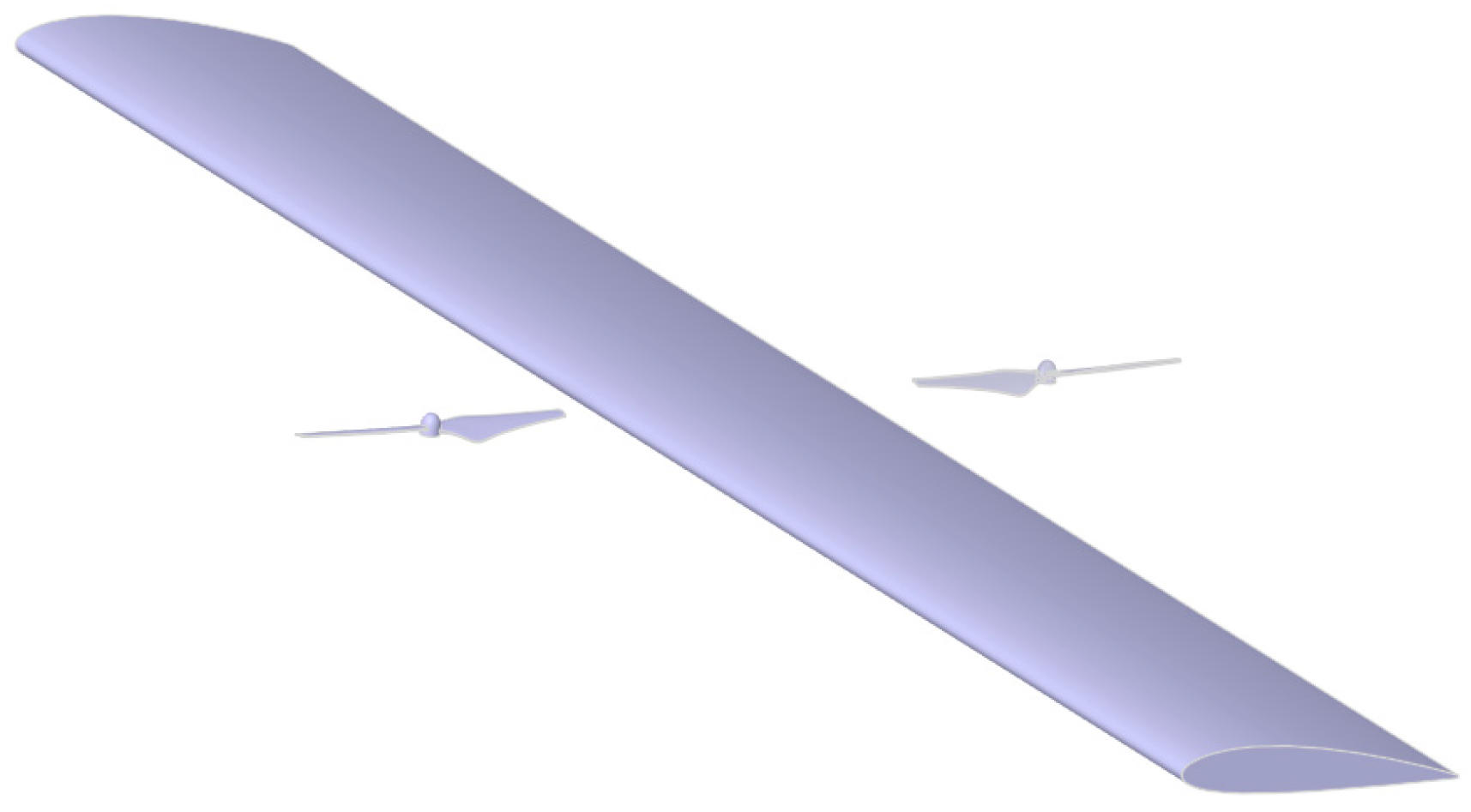
2.2. Computational Model

In this study, the fixed-wing chord length was 0.26 m, the length of the individual wings was 1.8 m, and the NACA2415 airfoil was used for the wings. The rotor model was DJI 9450 and the rotor radius was 0.12 m; these dimensions and models were taken from two relevant pieces of literature [31,32] to ensure the validity and accuracy of the models employed in this study. The rotor tip chord length was 0.012 m. Figure 2 illustrates the model used for the calculations.

2.3. Computational Domain

The computational domain used to study the aerodynamic interference of the rotor blades regarding the fixed wings was divided into three parts: the external flow field, rotational domain 1, and rotational domain 2. Figure 3 shows a schematic diagram of the computational area. According to the literature [33], the size of the external flow field should be 12–20 times the size of the research object. In this study, the external flow field was set as a rectangular domain of 4.8 m by 4.8 m, with the boundary conditions defined as the velocity inlet and pressure outlet. There were two rotating domains within the computational domain, each with a diameter of 0.25 m.

2.4. Mesh Generation

The mesh was divided into five computational domains: the external flow field region, the body of influence (BOI) in the external domain; the rotational domain; the BOI in the rotational domain; and the rotor. The meshing was performed using the Fluent Mesh software, with a maximum cell size of 0.5 m. The BOI in the rotational domain was used to better capture the rotor wake, and the BOI in the external domain was used to improve the computational accuracy. An interface was set between the outer side of the rotational domain and the inner side of the external flow field. Ten boundary layers were set on the rotor and fixed-wing surfaces, ensuring that y+ = 1. The overall mesh was a hybrid mesh generated from hexahedral and polyhedral cells. The mesh setup is shown in Figure 4.

2.5. Solver Settings

In this study, the Moving Reference Frame (MRF) method was used for the steady-state calculations, and the data from the steady-state calculations were used as the initial values for the transient calculations using the sliding mesh method. An interface was set between the rotating and non-rotating regions to exchange interpolated data. The simulations were performed using Fluent 2021R1, with the SST k-ω model selected for turbulence modeling. The semi-implicit method for pressure-linked equations (SIMPLE) was used for velocity and pressure coupling. For spatial discretization, second-order pressure discretization and a second-order upwind scheme were used for the turbulent kinetic energy, momentum equations, and turbulent dissipation terms. For temporal discretization, a second-order implicit upwind scheme was used, with each time step set to 2.0833333333 × 10⁻⁵ s, ensuring a Courant number < 5. Each time step corresponded to a 1° rotation of the rotor, and the maximum number of iterations per time step was set to 20 to ensure solver convergence. The velocity inlet was set to 5 m/s to simulate the low flight speed of the UAV when transitioning from VTOL to cruise. The angle of incidence of the fixed wing was set to 5°, and the rotational speeds of the front and rear rotors were both set to 8000 r/min.

2.6. Validation of Numerical Method

In this study, to validate the accuracy and reliability of the computational method, the rotors and fixed wings were first simulated. The fixed wing and rotor selected in this paper are based on the results of the existing literature [31,32], and the same fixed wing and rotor models are adopted to ensure the effectiveness and accuracy of the models used. The geometric model and mesh are shown in Figure 5. Figure 6 presents the lift coefficients for angles of attack from 0° to 10° and the lift for rotor speeds from 3000 r/min to 8000 r/min, with a comparison to the results in the literature. The overall error was within an acceptable range, indicating that the computational mesh and method used in this study had high accuracy and effectiveness.

2.7. Mesh Independence Study

To minimize the influence of the mesh on the computational results, a mesh independence study was conducted. This study established five computational grids, with grid counts of 3.4 million, 4.1 million, 5.22 million, 6.0 million, and 6.9 million, respectively. Figure 7 shows the variation in the total lift with the number of grid elements for the front and rear rotor and fixed wing. It can be seen that when the mesh count exceeded 5.2 million, the computed total lift values became stable and did not exhibit significant changes, indicating that the mesh count met the requirements. The subsequent calculations all used a mesh count of 5.2 million.

3. Results and Discussion

3.1. Setting of Rotor Position

To study the aerodynamic impact of the rotor position on the fixed wing, this study calculated the lift variations of the fixed wing with different positions of the front and rear rotors. To set the different positions of the rotors, the distance from the midpoint of the front rotor to the leading edge of the fixed wing was defined as L1; the distance from the midpoint of the rear rotor to the trailing edge of the fixed wing was defined as L2; and R was the rotor radius. By changing the values of R/L1 and R/L2, the positions of the front and rear rotors were varied. This setup is illustrated in Figure 8.

This study established nine computational models. Figure 9 illustrates the different positions of the front and rear rotors and the fixed wing, along with their physical significance. In Figure 9a–i, the position changes of the front and rear rotors with the fixed wing are shown. In these nine computational models, the size of the rotational domain, the mesh refinement, and the size of the external flow field were kept consistent.

3.2. Effect of Rotor Position on Magnitude of Fixed-Wing Lift and Drag

This study investigated the variation in the fixed-wing lift and drag with the spacing between the front and rear rotors and the fixed wing. When calculating the aerodynamic impact of the rotors on the fixed wing, the lift and drag of the fixed wing exhibited periodic variations. To facilitate the calculations and analysis, the average values of the instantaneous lift and drag of the fixed wing over three rotor rotations were used to denote the lift and drag of the fixed wing. Figure 10 shows the variations in the fixed-wing lift with changes in the rotor position. As shown in the figure, as the distance between the front rotor and the fixed wing increased, the lift of the fixed wing increased. Conversely, as the distance between the rear rotor and the fixed wing decreased, the lift of the fixed wing increased. Additionally, when the front rotor was positioned far from the fixed wing, a shorter distance between the rear rotor and the fixed wing resulted in a more significant increase in the fixed-wing lift. When the rear rotor was positioned far from the fixed wing, changes in the front rotor’s position had a smaller impact on the fixed-wing lift. Figure 11 shows the variations in the fixed-wing drag with changes in the rotor position. As shown in the figure, as the distance between the front rotor and the fixed wing increased, the drag of the fixed wing increased. As the distance between the rear rotor and the fixed wing decreased, the drag of the fixed wing increased.

Figure 12 and Figure 13 illustrate the pressure distributions on the upper and lower surfaces of the fixed wing with respect to the positions of the front and rear rotors. Upon comparing Figure 12a,e,i and Figure 13a,e,i, it can be found that the pressure distribution on the upper and lower surfaces of the fixed wing tended to be uniform when both the front and rear rotors were positioned far from the fixed wing, indicating that the aerodynamic influence of the rotors on the fixed wing was gradually weakened. This indicates that the rotor position had a significant effect on the pressure distribution of the fixed wing: the closer the rotor was to the fixed wing, the larger the effect; the further the rotor was from the fixed wing, the smaller the effect. From the boxed areas in Figure 12a and Figure 13a, it can be seen that when the rotor was close to the leading edge of the fixed wing, the upper and lower surfaces of the leading edge of the fixed wing produced a small, localized, positive-pressure region. From the boxed areas in Figure 12a,d,g and Figure 13a,d,g, it is evident that when the rear rotor was close to the trailing edge of the fixed wing, a negative-pressure area was formed on the upper surface near the trailing edge of the fixed wing, while a large, positive-pressure area was formed on the lower surface. Additionally, a localized high-pressure area was observed near the wingtip of the rear rotor. From the boxed areas in Figure 12d–f, it can be observed that as the distance between the rear rotor and the fixed wing increased, the negative-pressure areas on the upper surface of the fixed wing decreased. When comparing Figure 12e,f and Figure 13e,f, it is evident that the positive-pressure area on the trailing edge of the fixed wing’s upper surface increased significantly, while the pressure changes on the lower surface of the trailing edge were less pronounced. This indicates that when the rear rotor maintained a certain distance from the trailing edge of the fixed wing, changes in the position of the rear rotor had a greater impact on the pressure variation on the upper surface of the fixed wing than on the lower surface.

In order to further investigate the mechanism of the rotor position regarding the aerodynamic influence of the fixed wing, this study analyzed the rotor and fixed-wing surfaces from the perspective of the airflow streamlines, as shown in Figure 14. It is well-known that both the front and rear rotors will inhale the nearby airflow and change its initial flow direction. From Figure 14a,d,g, it can be seen that, when the front rotor approached the fixed wing, the airflow moving from left to right was influenced by the front rotor and changed its flow direction. This change caused the airflow between the front rotor and the leading edge of the fixed wing to approach the leading edge at an angle different from the initial 0-degree angle, resulting in a negative angle of attack at the leading edge of the fixed wing. When comparing Figure 15 (a), (d), (g), it can be seen that the closer the front rotor was to the leading edge of the fixed wing, the greater the extent of the negative angle of attack and the smaller the fixed-wing lift. Therefore, the closer the front rotor was to the leading edge of the fixed wing, the lower the fixed-wing lift. Additionally, when comparing Figure 16A,B, it is clear that the flow velocity on the lower surface of the trailing edge of the fixed wing increased as the distance between the rear rotor and the fixed wing increased. Therefore, it can be concluded that the front rotor affected the fixed-wing lift by influencing the airflow direction at the leading edge of the fixed wing, and the rear rotor affected the fixed-wing lift by influencing the airflow velocity at the lower surface of the trailing edge of the fixed wing.

3.3. Fluctuating Effects of Rotor on Lift and Drag in Fixed Wing

In this study, the change characteristics of the fixed wing’s lift and drag fluctuations in the transition phase in a compound-wing UAV were investigated, focusing on the analysis of the fixed wing’s lift and drag fluctuations and the changes in the upper and lower surface pressures when the rotor was in different phase angles in one rotation cycle. In Figure 17 and Figure 18, the curves with different colors represent the front and rear rotors at different positions, corresponding to cases (a) to (i) in Figure 18, respectively. Figure 17 and Figure 18 show the fluctuating changes in the fixed-wing lift and drag. From these figures, it can be seen that the fixed-wing lift and drag exhibited periodic fluctuations with the rotor’s rotation, and the shorter the distance between the front and rear rotors and the fixed wing, the greater the magnitude of the change in the lift and drag. This periodic change in the lift and drag will change the aerodynamic forces acting on the fixed wing during the transition phase, thus affecting the flight safety.

According to Figure 17(i) and Figure 18(i), the lift and drag fluctuations of the fixed wing were almost constant when the distances between the front and rear rotors and the fixed wing were R/L1 = 0.25 and R/L2 = 0.25. This indicates that the fixed wing will not be affected by the rotor wake in this configuration. Therefore, mounting the front and rear rotors at this position avoids fluctuations in the fixed-wing lift and drag due to the rotor wake during the transition phase. In addition, the curves in Figure 17 and Figure 18 show that, with fixed front and rear rotor positions, the instantaneous lift and drag of the fixed wing were minimized at rotor phase angles of 90° and 270°, while the instantaneous lift and drag of the fixed wing reached their maximum values at a phase angle of 180°. This shows that the fluctuations of the fixed wing were maximized at the rotor phase angles of 90°, 180°, and 270°.

The aerodynamic forces on the fixed wing will fluctuate due to the changes in the upper and lower surface pressures. Therefore, for the case with the smallest distance between the front and rear rotors and the fixed wing, as shown in Figure 16A, which is the case with the largest fluctuation in the aerodynamic force on the fixed wing, this study investigated the change in pressure on the upper and lower surfaces of the fixed wing with the phase angle of the rotors.

Figure 19 shows the pressure variations on the upper surface of the fixed wing when the rotor was at different phase angles during one rotation cycle. It can be seen that the pressure variation on the upper surface of the fixed wing in the phase angle range of 30° to 180° was consistent with that in the range of 180° to 360°, so only the range of 30° to 180° was analyzed. As shown in Figure 19a, when the front and rear rotor phase angles were 30°, a positive-pressure area was generated on the upper surface of the fixed wing near the front rotor, while a negative-pressure area was formed near the rear rotor tip at the trailing edge of the fixed wing. Figure 19b shows that when the phase angles of the front and rear rotors were 60°, a local high-pressure area was generated within the positive-pressure area on the upper surface of the leading edge of the fixed wing. As the rotor rotated, the low-pressure area on the upper surface of the trailing edge of the fixed wing decreased, and the localized high-pressure area on the upper surface of the leading edge of the fixed wing persisted from 90° to 150°, while the low-pressure area on the upper surface of the trailing edge was still located in the vicinity of the tip of the rear rotor. At 150°, the local high-pressure area on the leading edge of the fixed wing started to decrease, and the pressure on the trailing edge of the fixed wing near the tip of the rear rotor also started to decrease. When the phase angle of the front and rear rotor was 180°, the local high-pressure area on the leading and trailing edges of the fixed wing almost disappeared, the negative-pressure range of the upper surface of the fixed wing was the largest, and the total pressure on the upper surface reached the minimum.

In summary, the localized high-pressure area on the upper surface of the leading edge of the fixed wing initially increased as the front and rear rotors rotated from 30° to 180°; it then began to decrease at 150° and almost disappeared at 180°. At the same time, there was always a positive-pressure area near the front rotor on the upper surface of the leading edge of the fixed wing. The range of the negative-pressure area on the upper surface of the trailing edge of the fixed wing is mainly related to the position of the rear rotor tip. When the rotor tip is positioned far away from the fixed wing, the range of the negative-pressure area is smaller. When the front rear rotor is perpendicular to the wingspan direction, the range of the negative-pressure area on the upper surface of the trailing edge reaches the maximum, and the total pressure is the smallest.

Figure 20 shows the pressure variations on the lower surface of the fixed wing when the rotor was at different phase angles during a rotational cycle. As shown in the figure, when the rotor phase angle was between 30° and 120°, the range of the negative-pressure area on the lower surface of the fixed wing changed periodically depending on the rotor tip position. When the rotor phase angle was 150°, the negative-pressure area on the lower surface of the leading edge of the fixed wing was divided, and a small positive-pressure area started to form near the tip of the front rotor. When the rotor continued to rotate, the low-pressure area on the lower surface of the trailing edge of the fixed wing underwent periodic changes. When the phase angle of the rear rotor was 150°, the top of the rear rotor was adjacent to the trailing edge of the fixed wing, and the airflow at the trailing edge of the fixed wing formed a localized high-pressure area under the influence of the rear rotor. When the phase angle of the rear rotor was 180°, the localized high-pressure area on the lower surface of the trailing edge of the fixed wing reached its maximum. At the same time, the leading edge of the lower surface of the fixed wing was also affected by the front rotor to generate a local high-pressure area; at this time, the range of the negative-pressure area on the lower surface of the fixed wing reached the minimum, and the total pressure on the lower surface reached the maximum.

3.4. Discusstion

In summary, in the transition phase in the compound-wing UAV, the rotor position and phase angle have an effect on the magnitude of and fluctuations in the lift and drag on the fixed wings. The effect of the rotor position on the lift and drag of the fixed wings is as follows: when the distance between the front rotor and the fixed wing decreases, the fixed wing lift and drag decrease; and when the distance between the rear rotor and the fixed wing decreases, the fixed wing lift and drag increase. The influence of the rotor on the fluctuations in the fixed-wing lift and drag is as follows: the fixed-wing lift and drag fluctuate periodically with the rotation of the rotor; the fluctuations in the fixed-wing lift and drag decrease when the front and back of the rotor are located away from the fixed wing; and the wake generated by the rotor has little aerodynamic effect on the fixed wing when R/L1 = 0.25 and R/L2 = 0.25.

Upon comparing the calculation models described in

Table 2. The wing lift and total lift of the calculation models.

Model	Wing Lift (N)	Total Lift (N)
(a)	2.815	18.874
(b)	2.384	18.511
(c)	2.145	18.161
(d)	3.377	18.632
(e)	2.683	18.197
(f)	2.292	18.021
(g)	3.874	19.384
(h)	2.976	18.887
(i)	2.613	18.086

and

Table 3. The wing drag and total drag of the calculation models.

Model	Drag Lift (N)	Total Drag (N)
(a)	0.201	0.649
(b)	0.114	0.562
(c)	0.095	0.566
(d)	0.241	0.627
(e)	0.135	0.563
(f)	0.102	0.561
(g)	0.261	0.622
(h)	0.216	0.676
(i)	0.159	0.631

, it can be seen that a change in the front and rear rotor positions leads to a positive or negative influence on the magnitude of the fixed-wing lift and drag, but the influence on the magnitude of the total lift and total drag is smaller. Moreover, it can be seen from Figure 17 and Figure 18 that different rotor positions have a greater influence on the magnitude of the fluctuation in the fixed-wing lift and drag, and the fluctuations in the fixed wing have a significant influence on the flight safety. Therefore, in the design of compound-wing UAVs, the selection of the rotor mounting position should place a greater emphasis on the effect of the rotor on the fluctuations in the fixed-wing lift and drag, rather than the effect on the size of the total lift and total drag. In this study, it is suggested that the rotor mounting positions should be set as R/L1 = 0.25 and R/L2 = 0.25, which minimize the effect of the rotor wake on the lift and drag fluctuations of the fixed wing. It is worth noting that the aerodynamic characteristics of the compound-wing UAV during the transition phase are discussed in this study, and there are few related studies in the existing literature. Therefore, these results provide a new perspective for understanding the effects of rotor position on lift and drag fluctuations of fixed wings.

4. Conclusions

In this study, the aerodynamic influence of the rotor on the fixed wing in the transition phase in a compound-wing UAV was investigated using the RANS-based CFD method. Moreover, the magnitude of the lift and drag and the fluctuations of the fixed wing according to the rotor position and phase angle in the transition phase during low-speed flight were researched. The following conclusions were obtained.

(1)

The fixed wing’s lift and drag decreased with the decreasing distance of the front rotor; the fixed wing’s lift and drag increased with the decreasing distance of the rear rotor.

(2)

During the rotation of the rotor, the lift and drag fluctuations of the fixed wing changed periodically due to the influence of the rotor wake, and the fixed wing’s lift and drag fluctuations decreased as the distance between the front and rear rotors and the fixed wing increased.

(3)

During the design of the compound-wing UAV, the front and rear rotor mounting positions should be set as R/L1 = 0.25 and R/L2 = 0.25. With these values, it is possible to mitigate the lift and drag fluctuations of the fixed wing due to the rotor wake, while the total lift and total drag are only slightly changed.

The current model did not take into account the aerodynamic influence of the tail-thrust propeller on the fixed wing and rotor blades due to the long distance between the tail-thrust propeller and the fixed wing and rotor blades. However, during actual flight, this effect, although small, still exists. Further research will focus on the overall aerodynamic characterization of the tail-thrust propeller, fixed wing, and rotor.

References

1. Alsamhi, S.H.; Ma, O.; Ansari, M.S.; Almalki, F.A. Survey on Collaborative Smart Drones and Internet of Things for Improving Smartness of Smart Cities. IEEE Access 2019, 7, 128125–128152. [Google Scholar] [CrossRef]
2. Rejeb, A.; Abdollahi, A.; Rejeb, K.; Zailani, S.; Treiblmaier, H. Drones in agriculture: A review and bibliometric analysis. Comput. Electron. Agric. 2022, 198, 107017. [Google Scholar] [CrossRef]
3. Ghali, R.; Akhloufi, M.A. Deep learning approaches for wildland fires remote sensing: Classification, detection, and segmentation. Remote Sens. 2023, 15, 1821. [Google Scholar] [CrossRef]
4. Kinaneva, D.; Hristov, G.; Raychev, J.; Gadzhev, V. Early forest fire detection using drones and artificial intelligence. In Proceedings of the 2019 42nd International Convention on Information and Communication Technology, Electronics and Microelectronics (MIPRO), Opatija, Croatia, 20–24 May 2019; pp. 1060–1065. [Google Scholar]
5. Sungheetha, A.; Sharma, R. Real-time monitoring and fire detection using internet of things and cloud-based drones. J. Soft Comput. Paradigm 2020, 2, 168–174. [Google Scholar] [CrossRef]
6. Alsamhi, S.H.; Shvetsov, A.V.; Kumar, S.; Ansari, M.S.; Rajput, N.S.; Baker, T. UAV computing-assisted search and rescue mission framework for disaster and harsh environment mitigation. Drones 2022, 6, 154. [Google Scholar] [CrossRef]
7. Amukele, T. Current state of drones in healthcare: Challenges and opportunities. J. Appl. Lab. Med. 2019, 4, 296–298. [Google Scholar] [CrossRef]
8. Park, S.; Kim, H.T.; Lee, S.; Son, H.C.; Jeong, H.; Mohaisen, A. Survey on anti-drone systems: Components, designs, and challenges. IEEE Access 2021, 9, 42635–42659. [Google Scholar] [CrossRef]
9. Gregory, D. From a view to a kill: Drones and late modern war. Theory Cult. Soc. 2011, 28, 188–215. [Google Scholar] [CrossRef]
10. Yaacoub, J.P.; Noura, H.; Salman, O.; Chehab, A. Security analysis of drones systems: Attacks, limitations, and recommendations. Internet Things 2020, 11, 100218. [Google Scholar] [CrossRef]
11. Kai, J.M. Full-envelope flight control for compound vertical takeoff and landing aircraft. J. Guid. Control Dyn. 2024, 47, 1–17. [Google Scholar] [CrossRef]
12. Misra, A.; Jayachandran, S.; Kenche, S.; Sharma, M. A review on vertical take-off and landing (VTOL) tilt-rotor and tilt wing unmanned aerial vehicles (UAVs). J. Eng. 2022, 2022, 1803638. [Google Scholar] [CrossRef]
13. Sembiring, J.; Sasongko, R.A.; Bastian, E.I.; Hidayat, S. A deep learning approach for trajectory control of tilt-rotor UAV. Aerospace 2024, 11, 96. [Google Scholar] [CrossRef]
14. Anderson, R.B.; Marshall, J.A.; L’Afflitto, A. Constrained robust model reference adaptive control of a tilt-rotor quadcopter pulling an unmodeled cart. IEEE Trans. Aerosp. Electron. Syst. 2020, 57, 39–54. [Google Scholar] [CrossRef]
15. Filippone, A. Flight Performance of Fixed and Rotary Wing Aircraft; Elsevier: Oxford, UK, 2006. [Google Scholar]
16. Liu, Y. Vertical Takeoff and Landing Fixed-Wing UAV Design, Control, and Test. Master’s Thesis, Nanjing University of Aeronautics and Astronautics, Nanjing, China, 2018. [Google Scholar]
17. He, X.; Li, Y.; Zhu, F.; Yu, L. Development status and design and manufacturing key technology of foreign vertical take-off and landing unmanned aircraft. Fly. Missile 2016, 6, 22–27. [Google Scholar] [CrossRef]
18. Duan, H.; Zhao, C.; Wang, Q. Development of new vertical takeoff and landing unmanned aircraft. In Proceedings of the 2014 (Fifth) China UAV Conference; China Aeronautical Society: Beijing, China; Chinese People’s Liberation Army Air Force Equipment Department: Beijing, China; Chinese People’s Liberation Army Navy Aerospace Technology Department: Beijing, China; Aviation Industry Corporation of China: Beijing, China; Beijing University of Aeronautics and Astronautics: Beijing, China, 2014; p. 7. [Google Scholar]
19. Wei, Z.; Liu, F.; Yang, S. Development status and technical points of vertical take-off and landing fixed-wing UAV. Aircraft Design 2024, 44, 5–13. [Google Scholar] [CrossRef]
20. Garcia, A.J.; Barakos, G.N. Numerical simulations on the ERICA tiltrotor. Aerosp. Sci. Technol. 2017, 64, 171–191. [Google Scholar] [CrossRef]
21. Li, P.; Zhao, Q.; Wang, Z.; Wang, B. Highly-efficient CFD method for predicting aerodynamic force of tiltrotor in conversion mode. J. Nanjing Univ. Aeronaut. Astronaut. 2015, 47, 189–197. [Google Scholar]
22. Dong, D.; Yang, W. Transient response analysis of rotor/wing coupled during tiltrotor transition flight. J. Nanjing Univ. Aeronaut. Astronaut. 2006, 38, 361–366. [Google Scholar]
23. Hadytama, M.R.; Sasongko, R. Dynamics simulation and analysis of transition stage of tilt-rotor aircraft. Appl. Mech. Mater. 2016, 842, 251–258. [Google Scholar]
24. Wu, Z.; Li, C.; Cao, Y. Numerical simulation of rotor–Wing transient interaction for a tiltrotor in the transition mode. Mathematics 2019, 7, 116. [Google Scholar] [CrossRef]
25. Lin, K.; Qi, J.; Wu, C.; Tang, X. Control system design of a vertical take-off and landing unmanned aerial vehicle. In Proceedings of the 2020 39th Chinese Control Conference (CCC), Shenyang, China, 27–29 July 2020; pp. 6750–6755. [Google Scholar]
26. Gunarathna, J.; Munasinghe, R. Simultaneous execution of quad and plane flight modes for efficient take-off of quad-plane unmanned aerial vehicles. Appl. Sci. 2021, 1. [Google Scholar] [CrossRef]
27. Hangxuan, H.E.; Haibin, D. A multi-strategy pigeon-inspired optimization approach to active disturbance rejection control parameters tuning for vertical take-off and landing fixed wing UAV. Chin. J. Aeronaut. 2022, 35, 19–30. [Google Scholar]
28. Hernández-García, R.G.; Rodríguez-Cortés, H. Transition flight control of a cyclic tiltrotor UAV based on the Gain-Scheduling strategy. In Proceedings of the 2015 International Conference on Unmanned Aircraft Systems (ICUAS), Denver, CO, USA, 9–12 June 2015; pp. 951–956. [Google Scholar] [CrossRef]
29. Tang, S.; Liu, Z.; Zhou, Y.; Li, Z.; Guo, J. Investigation on aerodynamic performance of tandem wing UAV with rear wing dihedral. Trans. Beijing Inst. Technol. 2015, 35, 1211–1216. [Google Scholar]
30. Haci Sogukpinar, I.; Bozkurt, I. Implementation of different turbulence models to find the proper model to estimate aerodynamic properties of airfoils. AIP Conf. Proc. 2018, 1935, 020003. [Google Scholar]
31. Park, Y.M.; Jee, S. Numerical study on interactional aerodynamics of a quadcopter in hover with overset mesh in OpenFOAM. Phys. Fluids 2023, 35, 8. [Google Scholar]
32. Kenneth, E.; Pinkerton, R.M. The Characteristics of 78 Related Airfoil Sections from Tests in the Variable-Density Wind Tunnel; Report No. 460; National Advisory Committee for Aeronautics: Washington, DC, USA, 1933; p. 14.
33. Yang, L.; Wang, S.; Quan, B. Correlation analysis between key simulation parameters and numerical accuracy of subsonic outflow field. J. Mianyang Norm. Coll. 2024, 43, 16–24. [Google Scholar]
Figure 1. Compound-wing vertical take-off and landing fixed-wing unmanned aerial vehicle.
Aerospace 11 00945 g001
Figure 2. Illustration of rotary and fixed-wing computational models.
Aerospace 11 00945 g002
Figure 3. Computational domain for R1/L = 0.9, R2/L = 0.9: (a) top view; (b) left view.
Aerospace 11 00945 g003
Figure 4. Mesh of the entire domain.
Aerospace 11 00945 g004
Figure 5. Geometric Models and Meshes.
Aerospace 11 00945 g005
Figure 6. Comparison of calculation results with references: (a) variation in fixed-wing lift coefficient with angle of attack; (b) variation in rotor lift with RPM.
Aerospace 11 00945 g006
Figure 7. The lift change of wing and rotor with mesh.
Aerospace 11 00945 g007
Figure 8. Rotor and wing position parameter.
Aerospace 11 00945 g008
Figure 9. Rotor and wing positional relationships and physical meanings.
Aerospace 11 00945 g009
Figure 10. The variation in the wing lift with the rotor position.
Aerospace 11 00945 g010
Figure 11. The variation in the wing drag with the rotor position.
Aerospace 11 00945 g011
Figure 12. Pressure contours on the upper surfaces of the wing with different rotor positions: (a) R1/L = 0.9, R2/L = 0.9; (b) R1/L = 0.9, R2/L = 0.5; (c) R1/L = 0.9, R2/L = 0.25; (d) R1/L = 0.5, R2/L = 0.9; (e) R1/L = 0.5, R2/L = 0.5; (f) R1/L = 0.5, R2/L = 0.25; (g) R1/L = 0.25, R2/L = 0.9; (h) R1/L = 0.25, R2/L = 0.5; (i) R1/L = 0.25, R2/L = 0.25.
Aerospace 11 00945 g012
Figure 13. Pressure contours on the lower surfaces of the wing with different rotor positions: (a) R1/L = 0.9, R2/L = 0.9; (b) R1/L = 0.9, R2/L = 0.5; (c) R1/L = 0.9, R2/L = 0.25; (d) R1/L = 0.5, R2/L = 0.9; (e) R1/L = 0.5, R2/L = 0.5; (f) R1/L = 0.5, R2/L = 0.25; (g) R1/L = 0.25, R2/L = 0.9; (h) R1/L = 0.25, R2/L = 0.5; (i) R1/L = 0.25, R2/L = 0.25.
Aerospace 11 00945 g013
Figure 14. Streamline of airflow through rotor and wing surfaces at different rotor positions: (a) R1/L = 0.9, R2/L = 0.9; (b) R1/L = 0.9, R2/L = 0.5; (c) R1/L = 0.9, R2/L = 0.25; (d) R1/L = 0.5, R2/L = 0.9; (e) R1/L = 0.5, R2/L = 0.5; (f) R1/L = 0.5, R2/L = 0.25; (g) R1/L = 0.25, R2/L = 0.9; (h) R1/L = 0.25, R2/L = 0.5; (i) R1/L = 0.25, R2/L = 0.25.
Aerospace 11 00945 g014
Figure 15. Schematic diagram of the change in the angle of attack with a change in the front rotor position: (a) R1/L = 0.9, R2/L = 0.9; (d) R1/L = 0.5, R2/L = 0.9; (g) R1/L = 0.25, R2/L = 0.9.
Aerospace 11 00945 g015
Figure 16. (A,B) Detailed diagrams of (a,b) in Figure 14.
Aerospace 11 00945 g016
Figure 17. Variation in wing lift with rotor phase angle: (a) R1/L = 0.9, R2/L = 0.9; (b) R1/L = 0.9, R2/L = 0.5; (c) R1/L = 0.9, R2/L = 0.25; (d) R1/L = 0.5, R2/L = 0.9; (e) R1/L = 0.5, R2/L = 0.5; (f) R1/L = 0.5, R2/L = 0.25; (g) R1/L = 0.25, R2/L = 0.9; (h) R1/L = 0.25, R2/L = 0.5; (i) R1/L = 0.25, R2/L = 0.25.
Aerospace 11 00945 g017
Figure 18. Variation in wing drag with rotor phase angle: (a) R1/L = 0.9, R2/L = 0.9; (b) R1/L = 0.9, R2/L = 0.5; (c) R1/L = 0.9, R2/L = 0.25; (d) R1/L = 0.5, R2/L = 0.9; (e) R1/L = 0.5, R2/L = 0.5; (f) R1/L = 0.5, R2/L = 0.25; (g) R1/L = 0.25, R2/L = 0.9; (h) R1/L = 0.25, R2/L = 0.5; (i) R1/L = 0.25, R2/L = 0.25.
Aerospace 11 00945 g018
Figure 19. Variations in pressure contours on the upper surface of the wing with different rotor angles: (a) 30°; (b) 60°; (c) 90°; (d) 120°; (e) 150°; (f) 180°; (g) 210°; (h) 240°; (i) 270°; (j) 300°; (k) 330°; (l) 360°.
Aerospace 11 00945 g019
Figure 20. Variations in pressure contours on the lower surface of the wing with different rotor angles: (a) 30°; (b) 60°; (c) 90°; (d) 120°; (e) 150°; (f) 180°; (g) 210°; (h) 240°; (i) 270°; (j) 300°; (k) 330°; (l) 360°.
Aerospace 11 00945 g020