Three-Dimensional Flutter Numerical Simulation of Wings in Heavy Gas and Transonic Flutter Similarity Law Correction Method

Abstract

Wind tunnel testing is a crucial method for studying aircraft flutter. Using heavy gas as the wind tunnel medium can mitigate the escalating issue of test models being overweight as advanced aircraft develop. This paper employs an analytical method for numerical calculations of three-dimensional (3D) wing flutter based on fluid–structure interaction (FSI). Flutter calculations for the Goland wing are conducted, and the results in the air medium are consistent with the literature. In contrast, significant differences in flutter behavior are observed in the heavy gas R134a medium. Compared to air, when the model reaches a critical state in R134a, the incoming flow velocity is lower, the incoming flow density is approximately 3 to 5 times air, and the incoming flow dynamic pressure is about 1.1 to 1.2 times that of air. The correction of heavy gas flutter data is crucial for wind tunnel testing. This paper proposes a correction method based on the unsteady transonic flow similarity law proposed by Bendiksen under quasi-steady conditions. Attempts are made to revise relevant published wind tunnel tests and heavy gas flutter calculation results. The transonic flutter similarity law effectively explains the flutter similarity of rigid models in both heavy gas and air media. Still, it fails in cases with highly reduced frequencies and low mass ratios, such as those encountered with flexible wings.

1. Introduction

Flutter represents a significant challenge in the domain of aircraft aeroelasticity. Due to the interplay of structural inertia, elastic, damping, and aerodynamic forces, an aircraft can experience self-excited vibrations characterized by unattenuated amplitudes, commonly called flutter. During flutter events, the aircraft continuously extracts energy from the airflow, resulting in pronounced structural vibrations that can lead to failure. In aircraft design, considerable attention has been devoted to the issue of flutter [1].

Wind tunnel testing is a crucial methodology for investigating the flutter phenomenon in aircraft. Wind tunnel testing is grounded in similarity theory, which utilizes dynamic scale models to conduct experiments within wind tunnels. The results obtained from these tests can validate and enhance the aircraft’s structural design and performance metrics while also serving as a reference for related flight evaluations. Since the completion of the National Aeronautics and Space Administration’s (NASA) Transonic Dynamic Tunnel (TDT) for advanced aircraft, over 600 aeroelastic tests involving various aircraft configurations have been conducted [2], demonstrating that wind tunnel tests play a crucial role in type design, engineering applications, and numerical simulation calculations.

Conventional wind tunnel tests necessitate that both the test model and the actual aircraft adhere to a series of Similarity criteria, among which parameters such as Mach number M refer to Equation (1), mass ratio μ refer to Equation (2), and reduced frequency k refer to Equation (3) are critical factors influencing the flutter characteristics of aircraft.

$$M={\displaystyle \frac{U}{a}}$$

(1)

$$\mu ={\displaystyle \frac{m}{\pi \rho b^2}}$$

(2)

$$k={\displaystyle \frac{\omega b}{U}}$$

(3)

U is the velocity of flow, and a denotes the local sound speed in Equation (1). ρ signifies the fluid density traversing through the structure, and m refers to the mass per unit extension in Equation (2). b indicates the half chord length of the wing, and ω represents the natural frequency of the aircraft structure in Equation (3). Because the dimensions of the wind tunnel are conspicuously smaller than those of the actual aircraft, attaining mass ratio similarity proves arduous while guaranteeing that the scaled test model conforms to geometric similarity. The mass ratio of the fluid is markedly lower than that of the solid structure, thereby giving rise to a severely exacerbated problem of model overweight. The progression of future aircraft design persistently focuses on high efficiency, cost-effectiveness, longevity, and exceptional reliability, imposing increasingly rigorous comprehensive demands on materials and structures [3]. Lightweight composite material architectures are extensively employed to alleviate aircraft’s structural weight and enhance aeroelasticity [4]. On the other hand, in the quest for stealth capabilities, modern advanced combat aircraft prevalently adopt a flying-wing configuration [5]. The aerodynamic interdependency among the components of flying-wing aviation cannot be disregarded; thus, a full-scale flutter test is indispensable to determine both aerodynamic and flutter characteristics; all these novel requirements exacerbate the problem of excessive weight of test models to a greater extent.

Adopting heavy gases as the operational medium in wind tunnel tests can efficaciously mitigate the issue of overweight test models. Heavy gases typically denote polymeric gases whose molecular weight is approximately thrice that of air. Commonly employed heavy gas media encompass R12 (Freon, CCl2F2), R134a (tetrafluoromethane, CH2FCF3), and SF6 (sulfur hexafluoride, utilized as insulation gas in power plants), and so on.

Table 1. Comparison of thermodynamic parameters of heavy gas medium and air.

Title 1	Air	R12	R134a	SF6
Eelative molecular mass	29	121	102	146
Standard status density/(kg/m3)	1.29	5.40	4.55	6.52
Specific heat ratio γ	1.40	1.14	1.13	1.095
Viscosity coefficient	38.6	31.3	28.6	32.6
Speed of sound/(m/s)	340	154	165	134

exhibits a detailed comparative assessment of several thermodynamic parameters between the heavy gas medium and air.

Heavy gas media have low sound velocity and high density, which can effectively solve the problem of mass simulation in wind tunnel test aircraft. Concurrently, the heavy gas wind tunnel can effectively reduce the test model’s vibration frequency, augment the experimental data’s signal-to-noise ratio, prominently escalate the Reynolds number, curtail the power consumption of the compressor, and mitigate the operational expenditure and the like. The TDT wind tunnel in the United States is endowed with the capacity to operate within a heavy gas medium. Its technical ability of heavy gas wind tunnel test has made substantial contributions to the research on aircraft flutter technology [6], investigations on rotorcraft [7,8], explorations of space vehicles and launch vehicles [9], as well as research on active control of aerodynamic responses [10].

The ramifications of the thermodynamic dissimilarities between heavy gas medium and air, such as the variances in the ratio of specific heats, on wind tunnel tests constitute a matter that demands meticulous attention. In the 1960s, the TDT executed wind tunnel trials involving heavy gases and promulgated a fraction of the resultant test data. Moreover, they proposed amendment approaches like the area similarity law based on the streamline similarity in the nozzle flow test [11,12] and the transonic flow similarity criterion [13]. In recent years, the high-speed aerodynamic research endeavors of the China Aerodynamics Research and Development Center (CARDC) have delved into isentropic flow within heavy gas media [14], the Binary wing aerodynamics in heavy gas [15] and Correction of aerodynamics [16]. However, there is still a lack of relevant research on the flutter characteristics of heavy gas and the appropriate correction methods.

This paper, utilizing the analytical method based on FSI, conducts a numerical analysis of the 3D Goland wing model within a heavy gas, examining the variations in flutter characteristics induced by introducing heavy gas medium. At the same time, a correction method suitable for the flutter characteristics of heavy gas was established based on the unsteady transonic flutter similarity law proposed by Bendiksen [17,18] under the quasi-steady limit. The relevant TDT test data and calculation data, as well as the calculation data in this paper, were modified by using the established method. The application scope of the proposed correction method was studied.

2. Goland Wing Numerical Calculation Method

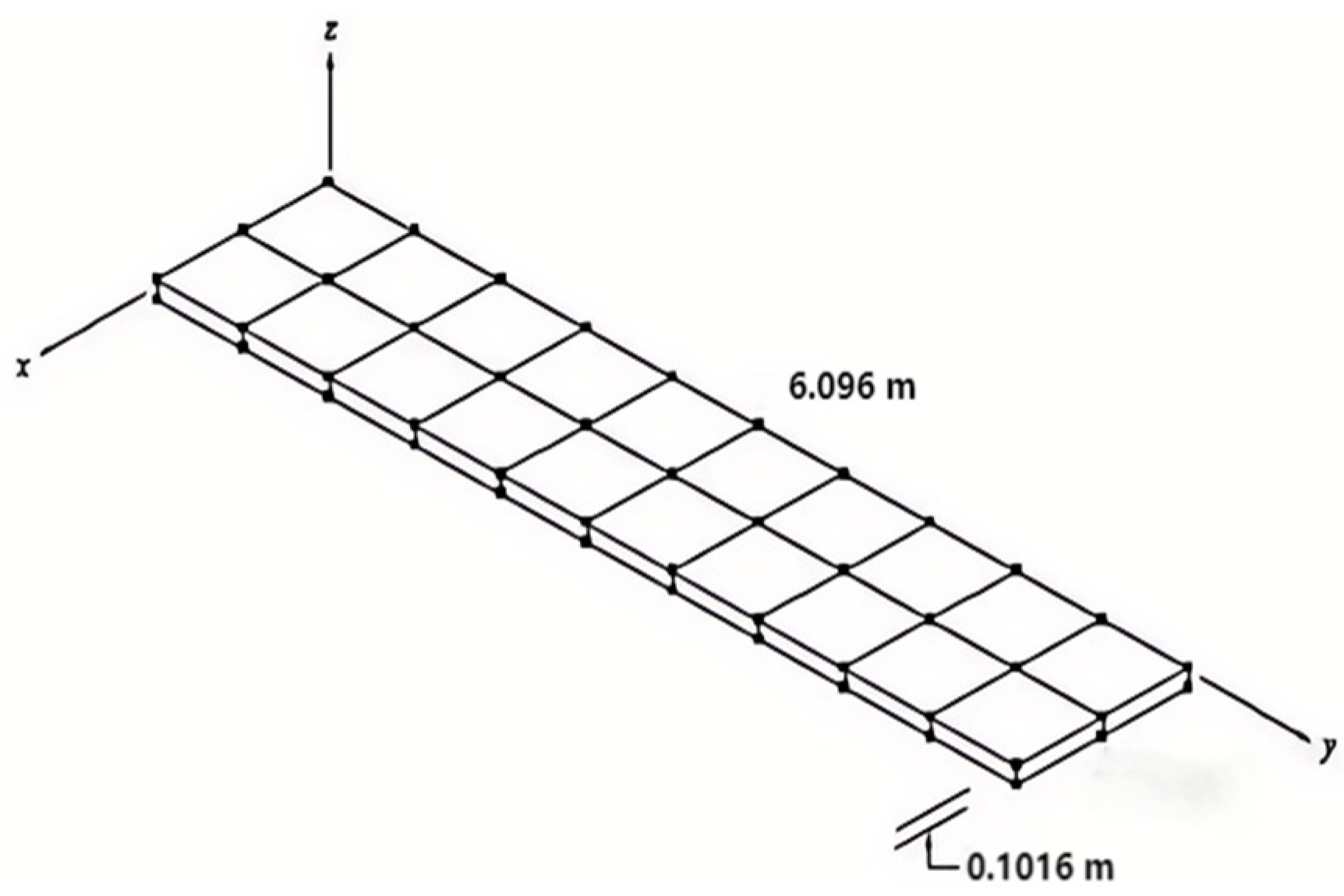
2.1. Structural

This paper employs a finite element model of the Goland wing, as illustrated in Figure 1. Martin Goland designed the Goland wing in 1945 [19], and it has been widely used to validate 3D flutter numerical calculation methods.

The Goland wing has a chord length of 1.8288 m and a half span of 6.096 m. The finite element model is a rectangular box structure beam extended in an infinite plane. The wing box model is a shear plate composed of 3 wing spars, each spaced at an interval of 0.6096 m (2 feet), and eleven wing ribs, each rib positioned at a height of 0.14016 m (4 inches). The elastic axis is 33% of the chord length from the wing’s leading edge, while the center of gravity is 44% of the chord length. The Goland model was fixed at the wing root.

Table 2. Structural parameters of Goland wing finite element model.

Parameter	Value	Parameter	Value
Young’s modulus E	2.307 × 10³ (GPa)	Shear modulus	8.65 × 102 (GPa)
Skin thickness of upper and lower surfaces (kg/m3)	4.7244 × 10−3 (m)	Thickness of front and rear edge spar	1.8288 × 10−4 (m)
Center spar thickness	2.7097 × 10−2 (m)	Thickness of wing ribs	1.0577 × 10−2 (m)
The area of the transition area	7.4322 × 10−5 (m2)	The area of the top area of the front and rear edge spar	3.8648 × 10−3 (m2)
The area of the top area of the center spar	1.3898 × 10−2 (m2)	The area of the top area of the wing rib	3.9205 × 10−3 (m2)

presents the other structural parameters.

Nastran2020 software was used to conduct modal analysis of the Goland wing model. Figure 2 shows the results of the first four natural modes of vibration.

Table 3. Comparison of mode frequencies across the initial four stages.

	This Paper	Liu Nan [20]	Rakesh Sarma [21]
mode 1	1.9836	1.98	1.98
mode 2	4.0501	4.05	4.04
mode 3	9.6965	9.69	9.68
mode 4	13.29	13.29	13.28

presents a comparison of the frequencies of the four modes shapes with those reported in existing literature. The results of comparison indicate that the Goland finite element model is accurate.

2.2. Fluid and FSI

The open-source computational fluid dynamics (CFD) solver SU2 was employed for flow numerical simulations. The structural information is provided to the SU2 through files with the extensions .f06 and .pch from Nastran. The analysis captures only the first four modes, with modal damping configured to zero. The internal module is established and activated through the configuration file su2.cfg.

The aerodynamic model is based on the compressible Reynolds-averaged Navier–Stokes (RANS), the conservation Equation of the RANS reads

$${\displaystyle \frac{\mathsf{\partial }}{\mathsf{\partial }t}}{\displaystyle \underset{\mathrm{\Omega }}{\int }W}\mathrm{d}\mathrm{\Omega }+{\displaystyle \underset{\mathsf{\partial }\mathrm{\Omega }}{\oint }(F_c-F_v)}\mathrm{d}S={\displaystyle \underset{\mathrm{\Omega }}{\int }Q\mathrm{d}\mathrm{\Omega }}$$

(4)

where W is conservative variables, F_c is a vector of the convective fluxes, F_v is a vector of the viscous fluxes, and Q is a source term, which comprises all volume sources due to body forces and volumetric heating. Meanwhile, t represents the time, S is the control volume surface area, Ω is the control volume, ∂Ω is the boundary of the control volume, the specific expression is as follows:

$$W=\left[\begin{array}{c}\rho \\ \rho u\\ \rho v\\ \begin{array}{c}\rho w\\ \rho E\end{array}\end{array}\right]F_C=\left[\begin{array}{c}\rho (n_{x}u+n_{y}v+n_{z}w)\\ \rho uV+n_{x}p\\ \rho vV+n_{y}p\\ \begin{array}{c}\rho wV+n_{z}p\\ \rho H_{t}V\end{array}\end{array}\right]F_v=\left[\begin{array}{c}0\\ n_x{\tau }_{xx}+n_y{\tau }_{xy}+n_z{\tau }_{xz}\\ n_x{\tau }_{yx}+n_y{\tau }_{yy}+n_z{\tau }_{yz}\\ \begin{array}{c}{n}_x{\tau }_{zz}+n_y{\tau }_{zy}+n_z{\tau }_{zz}\\ n_x{\mathrm{\Theta }}_x+n_y{\mathrm{\Theta }}_y+n_z{\mathrm{\Theta }}_z\end{array}\end{array}\right]Q=\left[\begin{array}{c}0\\ \rho f_{e.x}\\ \rho f_{e.y}\\ \begin{array}{c}\rho f_{e.z}\\ \rho f_e.v+q_h\end{array}\end{array}\right]$$

(5)

$$\begin{array}{c}{\mathrm{\Theta }}_x=u{\tau }_{xx}+v{\tau }_{xy}+w{\tau }_{xz}+\kappa \frac{\mathsf{\partial }T}{\mathsf{\partial }x}\\ {\mathrm{\Theta }}_y=u{\tau }_{yx}+v{\tau }_{yy}+w{\tau }_{yz}+\kappa \frac{\mathsf{\partial }T}{\mathsf{\partial }y}\\ {\mathrm{\Theta }}_z=u{\tau }_{zx}+v{\tau }_{zy}+w{\tau }_{zz}+\kappa \frac{\mathsf{\partial }T}{\mathsf{\partial }z}\end{array}$$

(6)

where u, v, and w are the components of the velocity vector in the x, y, and z coordinates; τ_ij, E, H_t, κ, q_h, and f_e are, respectively, the components of the stress tensor, the total energy per unit mass, total enthalpy, thermal diffusivity coefficient, time rate of heat transfer per unit mass, body force per unit volume; f_e.x, f_e.y, and f_e._z in Equation (5) denote the components of the f_e in the x, y, and z coordinates; and n_x, n_y, and n_z denote the components of the normal vector in the x, y, and z coordinates.

The RANS equation is spatially discretized using a finite volume method based on a lattice scheme. The implicit Euler method is used for time discretization. A central JST (Jameson–Schmidt–Turkel) scheme is used for the convective fluxes, and a weighted least square scheme is used for the gradients. The turbulence model is the SST (shear stress transport). The temporal increment is 0.0025 s, and the maximum physical elapsed time is 100 s.

The coupling strategy is loose coupling, and the structure and flow field information are transferred through the RBF radial basis function interpolation method. The radius of RBF is set to 6.5, and the calculation process is roughly as follows:

The initial attack angle of the Goland model is set at 0 degrees, and a non-reflecting far-field boundary condition is implemented.

(1)

The finite element model of the structure is established, and Nastran obtains the vibration mode and frequency information.

(2)

The structural information at time t_n is interpolated from the structural grid to the aerodynamic grid by RBF interpolation method.

(3)

Using dynamic mesh technology to update the pneumatic mesh, performing pseudo-time iteration until convergence.

(4)

The aerodynamic information at time t_n+1 is calculated and interpolated into the structural grid. The generalized and actual displacement on the structural grid at time t_n+1 are obtained by solving the structural Equation.

(5)

Determine whether the requirements for the end of calculation are met; if not, return to step 1 and repeat the iterative calculation.

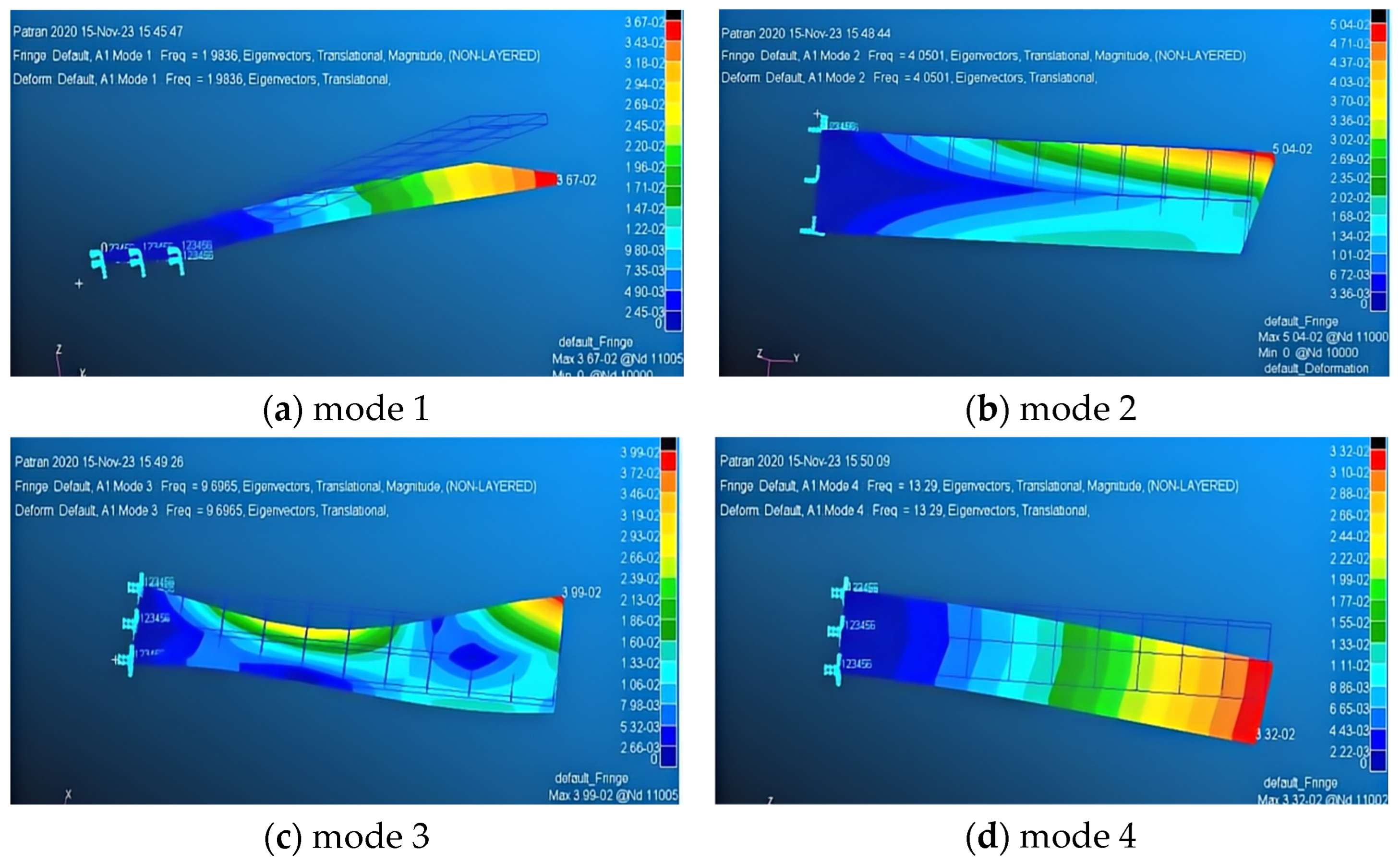
2.3. Verification of Algorithms

The flutter boundary of the Goland model is computed and compared with existing literature results to validate the accuracy of the numerical method. In the context of wind tunnel flow field control, the computational strategy is outlined as follows: a fixed incoming flow temperature of 288.15 K and a constant incoming flow Mach number are maintained, allowing for the derivation of the incoming flow flutter density “ρ_∞” curve across varying incoming flow Mach numbers “Ma_∞”, as illustrated in Figure 3.

The findings presented in this paper align closely with those reported by Rakesh Sarma. Simultaneously, the Goland model is associated with the critical flutter state at standard sea level conditions, specifically characterized by an air temperature of 288.15 K and a density of 1.225 kg/m³, where the Mach number is 0.420 and the velocity of flow reaches 142.92 m/s. As shown in

Table 4. Goland wing flutter results comparison.

Referencerefer	Modeling Approach	Flutter Velocity (m/s)
Goland and Luke	Analytical	137.25
Patil	Intrinsic beam + strip theory	135.25
This paper	Wingbox + RANS	142.92
Carmelo	Wingbox + 2-D unsteady aerodynamics	137.40

, the results derived from various methodologies exhibit slight discrepancies. For instance, the theoretical analysis conducted by Goland and Luke [22] yields a flutter velocity of 137.25 m/s, whereas Patil [23], utilizing intrinsic beam and strip theory, reports a flutter velocity of 135.60 m/s. Carmelo [24] adopted the same model as this paper and two-dimensional unsteady aerodynamics to obtain a flutter velocity of 137.40 m /s. The results obtained in this study fall within an acceptable margin of error, indicating that the algorithm used in this paper is appropriate for the numerical analysis of flutter in the Goland model.

3. Flutter of Goland Wing in Heavy Gas

R134a is used as the medium for calculating the flutter data of the Goland wing in a heavy gas environment, and its thermodynamic parameters are retrieved from the REFPROP9.1 software, which is developed by the National Institute of Standards and Technology (NIST) and dedicated to refrigerant physical property inquiries. As a typical non-ideal gas, R134a fails to comply with the ideal gas equation of state. Instead, the Peng–Robinson equation typically delineates its thermodynamic properties [25], as in Equation (7).

$$P={\displaystyle \frac{\mathrm{R}T}{\overline{v}-b}}-{\displaystyle \frac{\xi (T)}{\overline{v}(\overline{v}+b)+b(\overline{v}-b)}}$$

(7)

Herein, P, R, and T, respectively, denote the gas pressure, the gas constant, and the gas temperature; $\overline{v}$ denotes specific volume, while other parameters are elaborated in Equation (8).

$$\begin{array}{c}b={\displaystyle \frac{0.0778{\mathrm{RT}}_{\mathrm{c}}}{{\mathrm{P}}_{\mathrm{c}}}}\\ \xi (T)={\displaystyle \frac{0.45725{({\mathrm{RT}}_{\mathrm{c}})}^2}{{\mathrm{P}}_{\mathrm{c}}}}[1+f_w(1-\sqrt{T_r})]\\ f_w=0.37464+1.54226\omega -0.26992{\omega }^2\end{array}$$

(8)

Among these parameters, P_c and T_c represent the gas’s critical pressure and critical temperature, while T_r = T/T_c signifies the relative temperature, and ω refers to the gas molecule’s acentric factor.

The flutter characteristics of the Goland wing in an R134a were computed utilizing the same flutter analysis strategy as employed in air medium conditions. The temperature was maintained at 288.15 K, while the flow density was adjusted accordingly.

Table 5. The numerical calculation results of the Goland wing in R134a.

Mach number/M	0.421	0.550	0.650	0.750	0.880
Density/ρ (kg/m3)	6.962	3.641	2.439	1.696	1.049
flutter boundary/U (m/s)	66.8	88.0	104.3	120.6	141.7
Dynamic pressure/q (kpa)	15.533	14.098	13.266	12.334	10.531
speed of sound/a (m/s)	156.98	159.15	159.93	160.41	160.83
specific heat ratio/γ	1.132	1.122	1.118	1.115	1.114
Reynolds number/Re	4.07 × 107	2.80 × 107	2.22 × 107	1.79 × 107	1.30 × 107

shows the computational results for the R134a medium.

Table 6. The numerical calculation results of Goland wing in air.

Mach number/M	0.421	0.550	0.650	0.750	0.825	0.880
Density/ρ (kg/m3)	1.225	0.719	0.467	0.334	0.244	0.184
flutter boundary/U (m/s)	143.3	187.2	221.2	255.2	280.7	299.5
Dynamic pressure/q (kpa)	12.577	12.598	11.425	10.876	9.613	8.252
speed of sound/a (m/s)	340.40	340.37	340.35	340.34	340.34	340.33
specific heat ratio/γ	1.402	1.401	1.401	1.400	1.400	1.400
Reynolds number/Re	9.77 × 106	7.49 × 106	5.75 × 106	4.74 × 106	3.82 × 106	3.07 × 106

shows the computational results for the air medium to facilitate comparison.

The numerical calculation of the flutter behavior of the Goland wing in the R134a medium reveals significant differences compared to those observed in the air medium. In the conditions corresponding to the critical flutter state, the incoming flow density of the R134a medium is approximately three to five times greater than that of air, and the Reynolds number is roughly four to five times higher than that of air. The specific heat ratio and sound velocity for R134a and air demonstrate negligible variance with the Mach number under a constant air temperature of 288.15 K. Moreover, the specific heat ratio and velocity of sound of R134a are conspicuously lower than that of the airflow in air. The flutter boundary of the Goland wing within the heavy gas R134a exceeds that within the air. The incoming flow dynamic pressure within the R134a medium is approximately 1.1 to 1.2 times greater than that within the air medium; conversely, the free-stream velocity of the flutter boundary within the R134a medium is merely 0.4 to 0.5 times that within the air medium.

The disparity in flutter boundary and flow density also results in variations of critical parameters such as mass ratio and reduced frequency, thereby causing identical models to manifest disparate flutter characteristics in the air medium and the R134a medium.

4. Similarity Law for Transonic Flutter in Heavy Gases

In 1998, Bendiksen formulated the similarity law for unsteady transonic flow by employing the binary wing flutter model under quasi-steady conditions. The similitude law of unsteady transonic flow is established for the similarity parameter Ψ of transonic flutter in Equation (9).

$$\mathrm{\Psi }={\displaystyle \frac{{\overline{U}}^2}{\pi \mu {\left[\left(\gamma +1\right){M_{\infty }}^2\delta \right]}^{1/3}}}={\displaystyle \frac{\widehat{q}}{{\left[\left(\gamma +1\right){M_{\infty }}^2\delta \right]}^{1/3}}}$$

(9)

where δ is the thickness ratio of airfoil, γ is the specific heat ratio of gas, M_∞ is the incoming Mach number, $\overline{U}$ is shown in Equation (10), and $\widehat{q}$ is the dimensionless velocity pressure shown in Equation (11).

$$\overline{U}=U_{\infty }/b{\omega }_{\alpha }$$

(10)

$$\widehat{q}=q/{\displaystyle \frac{1}{2}}m{{\omega }_{\alpha }}^2={\displaystyle \frac{1}{2}}{\rho }_{\infty }{U_{\infty }}^2/{\displaystyle \frac{1}{2}}m{{\omega }_{\alpha }}^2={\displaystyle \frac{1}{\pi }}{\left({\displaystyle \frac{U_{\infty }}{b{\omega }_{\alpha }\sqrt{\mu }}}\right)}^2\hspace{0.33em}={\displaystyle \frac{1}{\pi }}{\left({\overline{U}}^{*}\right)}^2$$

(11)

where q is the flutter velocity pressure, U_∞ is the incoming flow velocity, ρ_∞ is the incoming flow density, and ω_α is the structure’s natural frequency. The similarity law for transonic is frequently utilized in the analysis of transonic flutter similarities across varying thickness ratios within the homologous airfoil. In the study of heavy gas flutter phenomena, similarity can be attained by utilizing airfoils with identical thickness ratios; similarity law for transonic flutter can be articulated through Equation (12) and Equation (13).

$${\psi }_{\mathrm{a}}={\psi }_h$$

(12)

$$\left({\displaystyle \frac{{\stackrel{⌢}{q}}_h}{{\stackrel{⌢}{q}}_a}}\right)={\left({\displaystyle \frac{\left({\gamma }_h+1\right){M_h}^2}{\left({\gamma }_a+1\right){M_a}^2}}\right)}^{1/3}$$

(13)

In the appeal equation, the subscript “a” denotes the corresponding parameter in the air medium, while the subscript “h” signifies the corresponding parameter in the heavy gas medium. The aerodynamic force, serving as a significant input parameter in the flutter, must not be disregarded. Liu of CARDC elaborates on the similarity law of transonic aerodynamic characteristics of the same thickness wing in heavy gas, as in Equations (14) and (15) [26].

$${\chi }_a={\chi }_h$$

(14)

$${\displaystyle \frac{1-M_{\mathrm{a}}^2}{{{\left[\right(1+\mathsf{\gamma }}_{\mathrm{a}}\left)M_{\mathrm{a}}^2\right]}^{2/3}}}={\displaystyle \frac{1-M_{\mathrm{h}}^2}{{{\left[\right(1+\mathsf{\gamma }}_{\mathrm{h}}\left)M_{\mathrm{h}}^2\right]}^{2/3}}}$$

(15)

where χ is the transonic aerodynamic similarity parameter. The transonic aerodynamic characteristics and flutter characteristics of the same wing in different media are expected to exhibit similarity; thus, Equations (12)~(15) must be concurrently satisfied. The relationship can be streamlined to Equations (16) and (17).

$${\displaystyle \frac{\left(1-{M_h}^2\right)/{M_h}^{4/3}}{\left(1-{M_a}^2\right)/{M_a}^{4/3}}}={\left({\displaystyle \frac{{\gamma }_h+1}{{\gamma }_a+1}}\right)}^{2/3}$$

(16)

$$\left({\displaystyle \frac{{\stackrel{⌢}{q}}_h}{{\stackrel{⌢}{q}}_a}}\right)={\left({\displaystyle \frac{\left({\gamma }_h+1\right){M_h}^2}{\left({\gamma }_a+1\right){M_a}^2}}\right)}^{1/3}$$

(17)

To ensure comparable aerodynamic characteristics, the specific heat ratio γ of the heavy gas medium differs from that of the air medium, necessitating the use of distinct Mach numbers for each medium; specifically, the M_h is marginally greater than the M_a. According to Equation (17), derived from the transonic flutter similarity law, the specific heat ratio of a heavy gas medium is typically lower than that of an air medium, and its actual dimensionless flutter velocity pressure boundary is also marginally lower than that of air.

Research on the aircraft flutter in a heavy gas must ensure that the reduced frequency k remains consistent with that observed in an air medium. Consequently, Equation (9) can be simplified as Equation (18).

$${\displaystyle \frac{{\mu }_h}{{\mu }_a}}={\left({\displaystyle \frac{\left({\gamma }_h+1\right){M_h}^2}{\left({\gamma }_a+1\right){M_a}^2}}\right)}^{1/3}$$

(18)

According to Equation (18), the mass ratio of a heavy gas needs to be slightly greater than that of air.

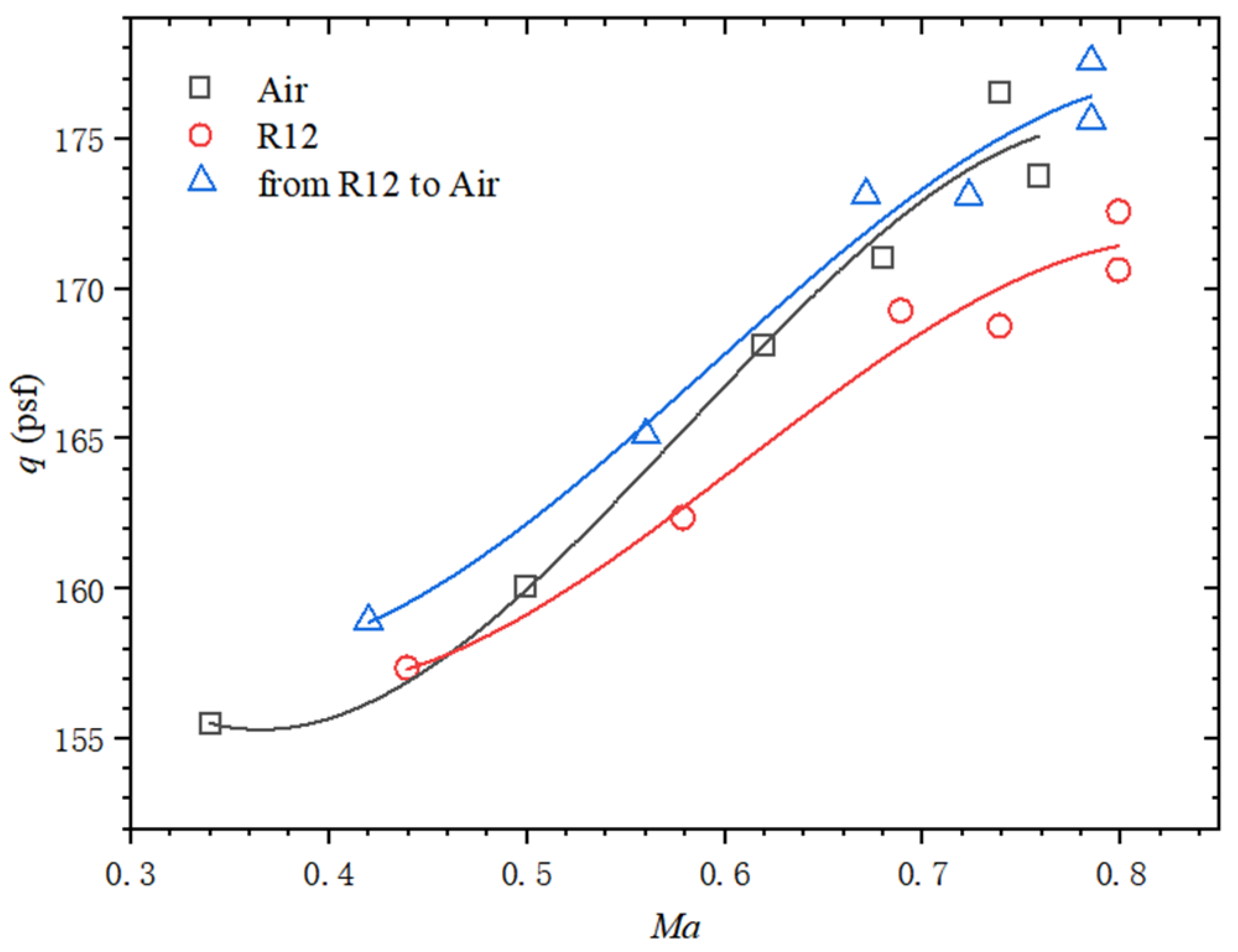
5. Correction of Flutter Data for Heavy Gas

Currently, the available data of heavy gas wind tunnel flutter tests and numerical calculations are minimal. This section attempts to rectify the sole dataset by employing the heavy gas transonic flutter similarity law. Some data are sourced from references, and the imperial units within those references remain unmodified (1 psf = 47.8803 Pa).

5.1. BSCW

In 1963, the Structural Dynamics Division of NASA’s Langley Research Center conducted flutter tests on the benchmark supercritical critical airfoil (BSCW) using a rigid body model within the pitch and plunge apparatus at the TDT [27]. The tests were performed in both air and R12 media. Simultaneously, a study [28] by the United States Air Force Academy reported numerical calculation results of BSCW in air and heavy gas media. The structural model employed for these calculations was identical to that used in the TDT test and incorporated findings related to the R134a medium. Figure 4 illustrates the results of flutter wind tunnel tests and numerical simulations for BSCW. The flutter boundary of the wing in a heavy gas is marginally lower than that observed in the air.

The transonic flutter similarity law is applied to rectify the wind tunnel test data for the R12 medium in Figure 5. The numerical simulation outcomes of the R134a medium are also calibrated in Figure 6. Based on the correction results presented in the figure, it can be concluded that modification of the transonic flutter similarity law methodology has a certain accuracy for the correction of the BSCW flutter boundary.

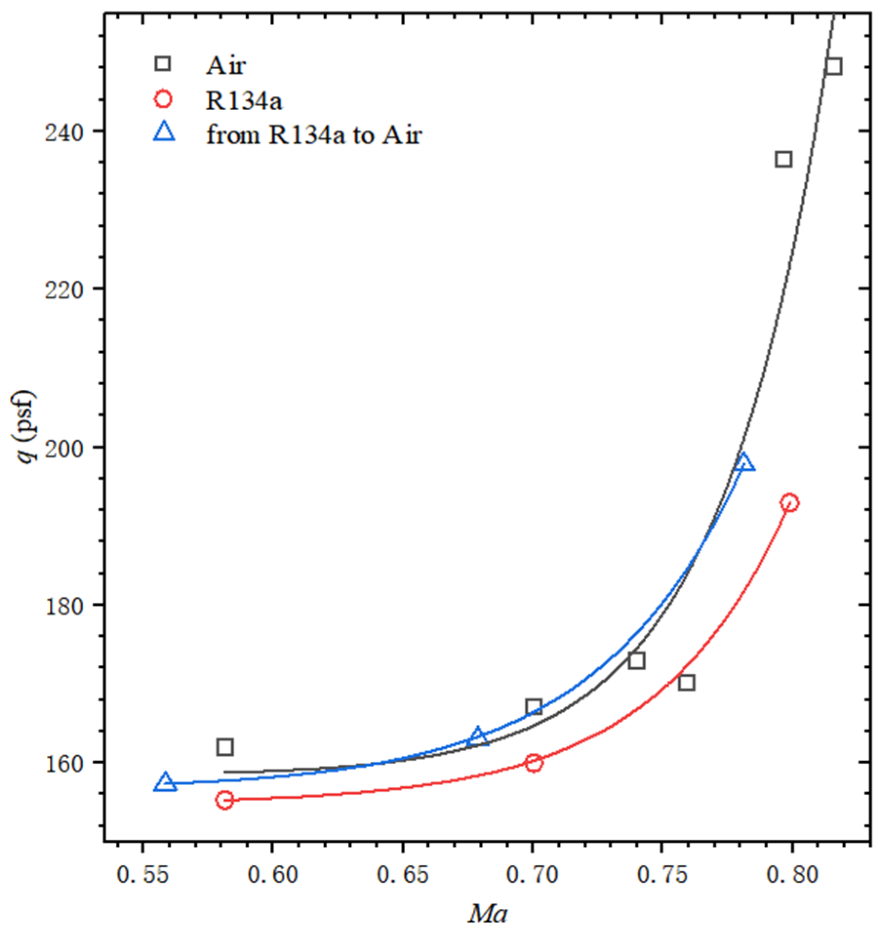
5.2. A 45° Sweptback Wing (NACA65A004)

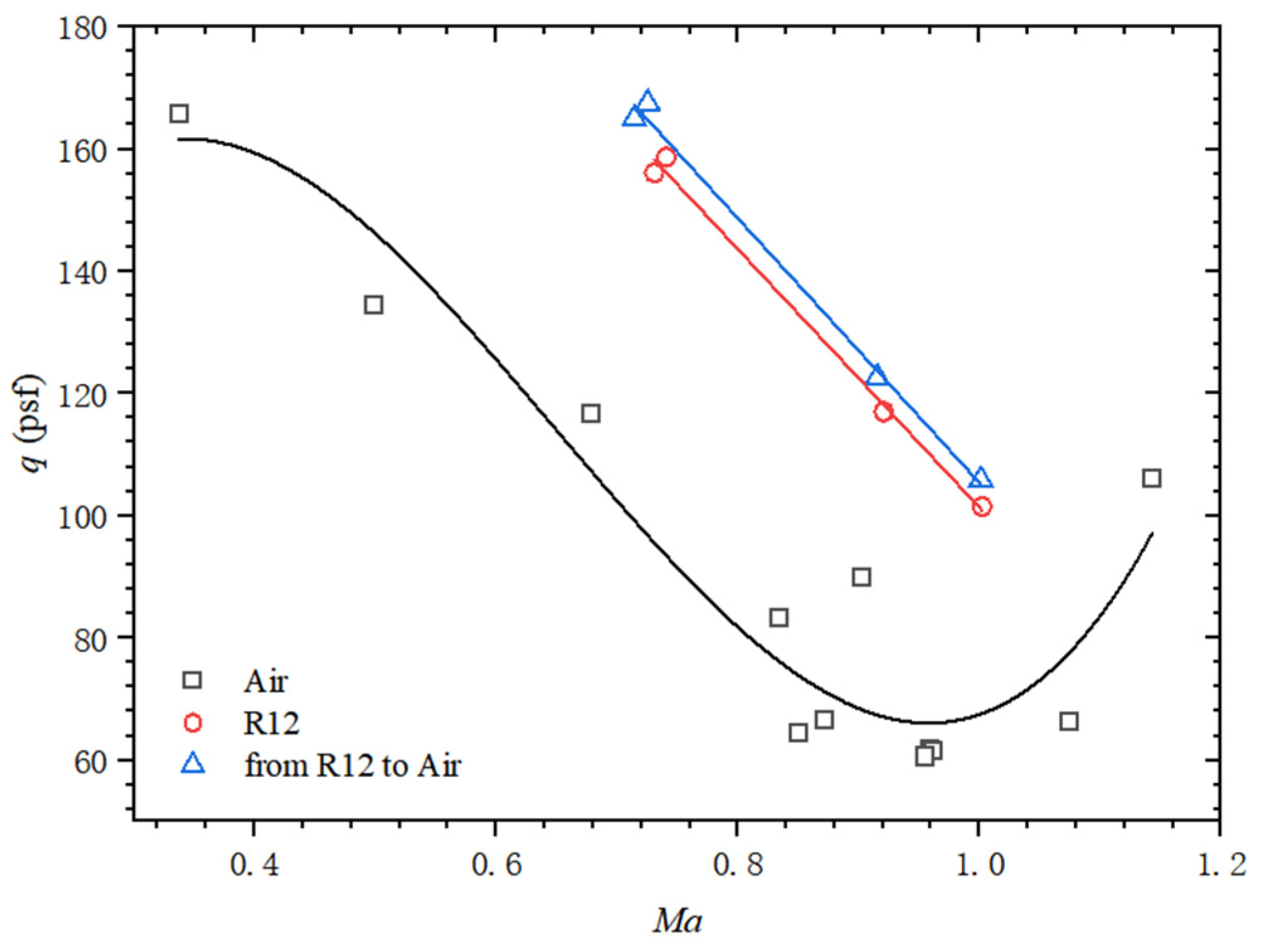
A 1963 report from NASA Langley documented a series of subsonic and transonic flutter tests conducted on a flexible wing with a 45°sweptback (NACA65A004) in the TDT and air and R12 media [29]. Figure 7 shows the results of flutter wind tunnel tests conducted in air and R12 medium and a revision of the R12 test data. In contrast to the previous rigid model, the transonic flutter boundary for the elastic wing in R12 is approximately twice that observed in air, and the transonic flutter similarity law does not adequately rectify the test data.

5.3. Goland Wing

The Goland wing employed in this study is also characterized as a flexible wing. Figure 8 shows the numerical results of the flutter boundary in both air and R134a medium, along with a revision of the R134a flutter data.

The transonic flutter similarity law is also suboptimal for correcting Goland wing flutter in a heavy gas environment. The numerical results show an opposite trend to the corrected results. The failure of the correction method can be attributed to two primary factors:

(1)

Compared with the binary rigid model, the flexible wing has more combined flutter modes. Due to the difference in mass ratio and reduced frequency, the dynamic characteristics of the model are different in air and heavy gas, and the flutter boundary has an opposite trend.

(2)

The transonic flutter similarity law is derived under quasi-steady conditions, neglecting the effects of unsteady aerodynamic derivatives. This approach is similar to the subsonic Theodorsen–Garrick theory and remains valid only at very low reduced frequencies and high mass ratios. Consequently, this may result in the inadequacy of the transonic flutter similarity law when applied to scenarios with high reduced frequencies and low mass ratios.

The transonic flutter similarity law can realize the flutter data similarity transformation well in some cases but fails in others, such as the flexible wing. A more comprehensive and sophisticated methodology is requisite for realizing the flutter data transformation in the heavy gas and air medium.

6. Conclusions

This paper presents a time-domain analysis method for the 3D flutter problem of the Goland wing, established through an analytical method based on FSI. The flutter boundary of the wing under conventional air medium conditions and the flutter velocity at standard sea level (142.92 m/s) are computed. The numerical results demonstrate strong agreement with existing literature.

The numerical simulation of the Goland flutter was conducted in a heavy gas environment using R134a as the medium. The results indicated that the flutter behavior in the R134a medium exhibited significant differences compared to that in the air. In the critical flutter state, the flutter boundary was lower than in the air. At the same time, the incoming flow density was approximately three to five times greater than that of air, and the dynamic pressure boundary ranged from about 1.1 to 1.2 times higher than that of air.

The correction of heavy gas flutter data is crucial for wind tunnel testing. This paper proposes a correction method based on the unsteady transonic flow similarity law proposed by Bendiksen under quasi-steady conditions. Furthermore, it revises the heavy gas wind tunnel test and numerical calculation results from the existing literature and the Goland numerical calculations presented herein. The transonic flutter similarity law elucidates the similarities observed in rigid models within heavy gas media and air; however, it does not account for the flutter similarities exhibited by flexible wings.

Further research is necessary to develop a comprehensive methodology for correcting wing flutter characteristics in heavy gas media.

References

1. Yu, Q.Y.; Yin, Y.P. Discussion on flutter of aircraft and bridge. Mech. Eng. 2023, 45, 721–727. [Google Scholar]
2. Robert, V.; Doggett. A Bibliography of Transonic Dynamics Tunnel (TDT) Publications; NASA Langley Research Center: Hampton, VA, USA, 2016. [Google Scholar]
3. Shi, G.H.; Wu, W.H.; Tao, R.; Luo, J.; Lin, H.; Li, Q.; Sun, Q. Application Requirement Analysis of Additive Manufacturing Technology in Aircraft Structure. J. Mech. Eng. 2024, 60, 74–84. [Google Scholar]
4. Corrado, G.; Ntourmas, G.; Sferza, M.; Traiforos, N.; Arteiro, A.; Brown, L.; Chronopoulos, D.; Daoud, F.; Glock, F.; Ninic, J.; et al. Recent progress, challenges and outlook for multidisciplinary structural optimization of aircraft and aerial vehicles. Prog. Aerosp. Sci. 2022, 135, 100861. [Google Scholar] [CrossRef]
5. Zhang, W.; Zhao, K.; Xia, L.; Gao, Z. A multi-disciplinary global/local optimization method for flying-wing airfoils design. Acta Aerodyn. Sin. 2021, 39, 37–52. [Google Scholar]
6. Perry, B.; Thomas, E.N. Activities in Aeroelasticity at NASA Langley Research Center. NASA Langley Res. Cent. 1997, 53, 77–88. [Google Scholar]
7. Yeager, J.W.T.; Kvaternik, R.G. Contributions of the Langley Transonic Dynamics Tunnel to Rotorcraft Technology and Development. In Proceedings of the AIAA Dynamics Specialists Conference, Atlanta, GA, USA, 5–6 April 2000; p. 1771. [Google Scholar]
8. Yeager, J.W.T. A Historical Overview of Aeroelasticity Branch and Transonic Dynamics Tunnel Contributions to Rotorcraft Technology and Development; NASA: Washington, WA, USA, 2001; TM-2001-211054. [Google Scholar]
9. Cole, S.; Keller, D.; Piatak, D. Contributions of the NASA Langley Transonic Dynamics Tunnel to launch vehicle and spacecraft development. In Proceedings of the AIAA Dynamics Specialists Conference, Atlanta, GA, USA, 5–6 April 2000; p. 1772. [Google Scholar]
10. Perr, B.; Noll, T.; Scott, R. Contributions of the Transonic Dynamics Tunnel to the testing of active control of aeroelastic response. In Proceedings of the AIAA Dynamics Specialists Conference, Atlanta, GA, USA, 5–6 April 2000; p. 1769. [Google Scholar]
11. Schuster, D.M.; Liu, D.D.; Huttsell, L.J. Computational aeroelasticity: Success, progress, challenge. J. Aircr. 2003, 40, 843–856. [Google Scholar] [CrossRef]
12. Fu, Q.; Zhang, X.; Zhao, M.; Zhang, C.H.; He, W. Research progress on the wind tunnel experiment of a bionic flapping-wing aerial vehicle. Chin. J. Eng. 2022, 44, 767–779. [Google Scholar]
13. Anders, J.B.; Anderson, W.K.; Murthy, A.V. Transonic similarity theory applied to a supercritical airfoil in heavy gas. J. Aircr. 1999, 36, 957–964. [Google Scholar] [CrossRef]
14. Liu, Y.P.; Kou, X.P.; Zha, J.; Yu, L.; Lu, B. The isentropic flow characteristics of heavy gas medium. J. Aerosp. Power 2023.
15. Zha, J.; Zeng, K.C.; Kou, X.P.; Yang, X.; Zhang, H. Transonic flow characteristics of supercritical airfoil in heavy gas medium. J. Aerosp. Power. 2021, 36, 1894–1905. [Google Scholar]
16. Liu, Y.P.; Zha, J.; Hu, Z.; Kou, X.P.; Yu, L.; Lu, B. Correction of Aerodynamic Characteristics in Heavy Gas Medium. J. Aerosp. Power, 2024; accepted. [Google Scholar]
17. Bendiksen, O.O. Transonic Similarity Rules for Flutter and Divergence. In Proceedings of the 39th AIAA/ASME/ASCE/AHS/ASC Structures, Structural Dynamics, and Materials Conference and Exhibit, Long Beach, CA, USA, 20–23 April 1998; p. 1726. [Google Scholar]
18. Bendiksen, O.O. Improved similarity rules for transonic flutter. In Proceedings of the 40th Structures, Structural Dynamics, and Materials Conference and Exhibit, St. Louis, MO, USA, 12–15 April 1999; p. 1350. [Google Scholar]
19. Goland, M. The Flutter of a Uniform Cantilever Wing. J. Appl. Mech. 1945, 12, 197–208. [Google Scholar] [CrossRef]
20. Liu, N. Investigation of Transonic Nonlinear Flutter and Efficient Analysis Approach; Northwestern Polytechnical University: Xi’an, China, 2016; pp. 73–74. [Google Scholar]
21. Sarma, R.; Dwight, R.P. Uncertainty Reduction in Aeroelastic Systems with Time-Domain Reduced-Order Models. AIAA J. 2017, 55, 2437–2449. [Google Scholar] [CrossRef]
22. Goland, M.; Luke, Y.L. The flutter of a uniform wing with tip weights. J. Appl. Mech. 1948, 15, 13–20. [Google Scholar] [CrossRef]
23. Patil, M.J.; Hodges, D.H.; Cesnik, C.E. Nonlinear aeroelastic analysis of complete aircraft in subsonic flow. J. Aircr. 2000, 37, 753–760. [Google Scholar] [CrossRef]
24. Carmelo, R.V.; Giuseppe, M.; Antonio, E.; Orlando, C.; Alaimo, A. An aeroelastic beam finite element for time domain preliminary aeroelastic analysis. Mech. Adv. Mater. 2023, 30, 1064–1072. [Google Scholar]
25. Poling, B.E.; Prausnitz, J.M.; O’connell, J.P. The Properties of Gases and Liquids; The McGRAW-Hill Companies: New York, NY, USA, 2001; Volume 5. [Google Scholar]
26. Liu, Y.P.; Xia, H.Y.; Zha, J.; Yu, L.; Lu, B. A Survey of the Test Data Correction Method in Heavy Gas Wind Tunnel. J. Aerosp. Power, 2024; accepted. [Google Scholar]
27. Bryan, E.; Dansberry, M.H.; Robert, M. Experimental unsteady pressures at flutter on the Supercritical Wing Benchmark Model. In Proceedings of the 34th Structures, Structural Dynamics and Materials Conference, La Jolla, CA, USA, 19–22 April 1993; p. 1592. [Google Scholar]
28. Jirasek, A.; Seidel, J. Study of Benchmark Super Critical Wing at Mach 0.8. In Proceedings of the AIAA SciTech Forum and Exposition, San Diego, CA, USA, 3–7 January 2022; p. 175. [Google Scholar]
29. Foughner, J.T., Jr.; Land, N.S.; Yates, E.C., Jr. Measured and Calculated Subsonic and Transonic Flutter Characteristics of a 45 Deg Sweptback Wing Planform in Air and in Freon-12 in the Langley Transonic Dynamics Tunnel; NASA: Washington, WA, USA, 1963; NASA-TN-D-1616.
Figure 1. Goland wing box model, left end fixed.
Aerospace 11 00932 g001
Figure 2. The results of the first four mode shapes.
Aerospace 11 00932 g002
Figure 3. The incoming flow flutter density curve in air.
Aerospace 11 00932 g003
Figure 4. The results of flutter wind tunnel tests and numerical calculation for BSCW.
Aerospace 11 00932 g004
Figure 5. Correction of R12 flutter wind tunnel test data (BSCW).
Aerospace 11 00932 g005
Figure 6. Correction of R134a flutter numerical calculation data (BSCW).
Aerospace 11 00932 g006
Figure 7. Correction of R12 flutter wind tunnel test data (a 45° sweptback wing).
Aerospace 11 00932 g007
Figure 8. Correction of R134a flutter numerical calculation data (Goland Wing).
Aerospace 11 00932 g008