A Convolution Auto-Encoders Network for Aero-Engine Hot Jet FT-IR Spectrum Feature Extraction and Classification

Abstract

Aiming at classification and recognition of aero-engines, two telemetry Fourier transform infrared (FT-IR) spectrometers are utilized to measure the infrared spectrum of the areo-engine hot jet, meanwhile a spectrum dataset of six types of areo-engines is established. In this paper, a convolutional autoencoder (CAE) is designed for spectral feature extraction and classification, which is composed of coding network, decoding network, and classification network. The encoder network consists of convolutional layers and maximum pooling layers, the decoder network consists of up-sampling layers and deconvolution layers, and the classification network consists of a flattened layer and a dense layer. In the experiment, data for the spectral dataset were randomly sampled at a ratio of 8:1:1 to produce the training set, validation set, and prediction set, and the performance measures were accuracy, precision, recall, confusion matrix, F1 score, ROC curve, and AUC value. The experimental result of CAE reached 96% accuracy and the prediction running time was 1.57 s. Compared with the classical PCA feature extraction and SVM, XGBoost, AdaBoost, and Random Forest classifier algorithms, as well as AE, CSAE, and CVAE deep learning classification methods, the CAE network can achieve higher accuracy and efficiency and can complete the spectral classification task.

1. Introduction

Airplane fault detection is a critical issue in the aviation industry and is essential for ensuring flight safety. Traditional methods of fault detection primarily rely on sensor monitoring and mechanical inspections, but these approaches have limitations regarding their limited detection range and difficulty in detecting early-stage faults. With the advancement of infrared spectroscopy technology, utilizing aero-engine hot jet infrared spectral classification for airplane fault detection has become an effective method. The infrared spectra present in the hot jet of aero-engines contain information about fuel composition and combustion processes. By analyzing and classifying different types of aero-engine hot jets’ spectra, faulty aero-engines can be quickly identified.

The classification characteristics of aero-engines are associated with the fuel type, combustion method, and emission properties. Various types of aero-engines generate hot plumes containing gaseous components and emissions post-combustion. The material molecules in the hot jet exhibit vibrational and rotational motions, giving rise to a distinct infrared spectrum. Infrared spectroscopy [1,2,3] is a technique used to examine the unique spectrum fingerprints generated by molecules when subjected to infrared radiation. Infrared spectroscopy helps in the analysis and identification of chemical bonds and molecular structures, ultimately allowing for the classification of aero-engines. The Fourier Transform Infrared Spectrometer (FT-IR Spectrometer) [4] is a significant method for the measurement of infrared spectra, facilitating the acquisition and conversion of interferograms of light signals in the wavelength range from 2.5 to 12 μm into continuous spectral data within a matter of seconds. Due to its capability to continuously, multi-directionally, and remotely measure and analyze targets in real-time, the FT-IR spectrometer has emerged as the preferred choice for conducting research on thermal radiation spectra in aero-engines.

Feature extraction and classification applications of infrared spectroscopy are currently prominent research areas. Classical methods for spectral feature extraction include wavelet transform (WT), principal component analysis (PCA), sparse representation, and auto-encoders (AE). In the field of deep learning, convolutional neural networks (CNNs), recurrent neural networks (RNNs), long short-term memory (LSTM) networks, and Transformer models have gained significant attention. Among these techniques, AE [5] are a widely adopted approach used for flexible feature extraction and dimensionality reduction that can effectively integrate various types of neural network structures such as CNNs, RNNs, and LSTMs to adapt to diverse data inputs. Common variations of AE models encompass stacked autoencoders (SAE), convolutional autoencoders (CAE), semi-supervised autoencoders (SSAE), generative adversarial encoders (GAE), etc. Furthermore, AEs have demonstrated successful applications in hyperspectral image (HSI) classification tasks. Chen [6] proposed a single-layer AE specifically designed for HSI classification. Kemker [7] compared the effectiveness of ICA features with Convolutional Autoencoders (CAE) and Stacked Convolutional Autoencoders (SCAE) in HSI classification. Duan [8] constructed three types of AE networks combined with transfer learning for near-infrared spectral analysis. Ma [9] improved the Deep Autoencoder (DAE) by incorporating regularization and contextual information, proposing a Spatially Updated Deep Autoencoder (SDAE) for spectral feature extraction. Zhao [10] used SAE for dimensionality reduction, employing 3D deep residual network. Wang [11] used the masked autoencoder framework (MAE) to complete hyperspectral image classification. Previous research [12] had already studied the suitability of the CNN framework for the author’s hyperspectral data set, so using the CAE network structure would have better feature extraction effects. Variants of CAE include Convolutional Variational Auto-Encoder (CVAE), Convolutional Sparse Autoencoder (CSAE), and ConvLSTM [13]. The CAE network model has also made further advancements in HSI processing tasks, as shown by Mei [14], who combined one-dimensional spectra with two-dimensional image information to construct a 3D-CAE network. Zhang [15] integrated local and global features by combining 3D-CAE with lightweight Transformers to capture nonlinear characteristics of spectra. Patel [16] utilized AE for enhancing image features, combining shallow CNNs for feature extraction and classification. Cao [17] employed CAEs to extract deep subspace representations while enhancing edge consistency through graph convolutional networks to improve semi-supervised convolutional neural networks’ classification performance. Chen [18], on the other hand, proposed the SCAE-MT classification method by combining SCAEs with transfer learning techniques. Zeng [19], meanwhile, combined deep subspace clustering with CAE for band selection purposes. Therefore, this paper aims to combine the advantages of AE feature learning and CNN local feature extraction to construct a CAE specifically designed for infrared spectral feature extraction and classification. While CAE demonstrates robust feature extraction capabilities, it is associated with significant computational resource consumption and faces challenges related to excessive memory usage when dealing with complex datasets. Furthermore, the current dataset was acquired under conditions of high signal-to-noise ratio, raising an important question regarding CAE’s ability to extract latent features in scenarios characterized by weak signals.

Given the limited availability of infrared spectral data for aero-engine hot jets, this study employs an experimental approach to measure the infrared spectra of six different types of aero-engine hot jet and generate a comprehensive spectral dataset. The paper proposes a CAE network for efficient extraction and classification of spectral features. The encoder network consists of three convolutional layers and three max-pooling layers, while the decoder network comprises three up-sampling layers and three deconvolution layers with symmetrical structure. The classification network predicts class labels based on the features extracted by the encoder through flattened and dense layers. Additionally, comparative experiments are conducted between CAE features and PCA features using Support Vector Machines (SVM), XGBoost, AdaBoost, and Random Forest classifiers. Furthermore, the performance of the CAE spectral classification network is compared with AE, CSAE, and CVAE networks. Experimental results demonstrate that the proposed CAE spectral classification network achieves an impressive accuracy rate of 96% with a running speed as fast as 1.57 s.

The main contributions of this paper can be summarized as follows:

(1) Paper presents a novel approach for measuring aero-engine hot jets using infrared spectroscopy, which is crucial for aero-engine classification and identification. Aero-engine hot jets emit important infrared radiation that can be captured by FT-IR spectrometers to provide molecular-level feature information. Use of the infrared spectrum for aero-engine classification is more scientific.

(2) The CAE spectrum feature extraction and classification network is developed to extract features from the aero-engine hot jets and employs a hybrid learning method to separately train the network for spectrum data reconstruction and classification prediction.

(3) Apply classical PCA, classifiers, AE, and their variants CSAE and CVAE to the classification task of infrared spectral data set of aero-engine hot jets.

The structure of this paper comprises five parts: Section 1 outlines the research background, summarizes current spectrum classification methods and AE research, and briefly describes the method, contribution, and structure of this paper. Section 2 provides a detailed explanation of the principle behind aero-engine hot jet infrared spectrum classification and datasets. Section 3 covers feature extraction and classification networks, including an overview of network design, the CAE network components, as well as training and prediction methods used in the network. In Section 4, experiment results are analyzed using performance measures to assess and interpret these methods. Comparative experiments were conducted on spectral classification using the classical PCA feature combined with SVM, XGBoost, AdaBoost, and Random Forest methods. Additionally, deep learning methods utilizing AEs and their variants were also employed for spectral classification experiments. In Section 5, this paper is summarized.

2. Classification Principle and Data Set of Aero-Engine Hot Jet Infrared Spectrum

Section 2 explains the classification principles of the aero-engine hot jet infrared spectrum, mainly including molecular rotation and the classification principles of the aero-engine hot jet infrared spectrum, as well as the infrared spectrum dataset of aero-engine hot jets.

2.1. Classification Principles of Aero-Engine Hot Jet Infrared Spectrum

Aero-engines are categorized into piston aero-engines and jet aero-engines. The former is seldom observed in contemporary aircraft due to its low efficiency, whereas the latter is the prevalent engine type in modern aircraft. Other studies also mention that the aforementioned aero-engines refer to jet aero-engines. Jet aero-engines can be classified into turbojet, turbofan, and turboprop types, all of which comprise an intake duct, compressor, combustion chamber, turbine, and exhaust nozzle. Figure 1 shows a schematic diagram of a jet aero-engine’s structure.

The operational procedure of an aero-engine is as follows: First, atmospheric air enters through the intake duct and undergoes compression by the compressor, resulting in elevated pressure and temperature. Subsequently, the compressed air enters the combustion chamber where it combines with fuel and undergoes combustion, releasing a substantial amount of energy while increasing the temperature. The high-temperature, high-pressure gas generated from this process then proceeds through turbine expansion to drive the turbine at a rapid rotational speed, subsequently propelling the compressor. Finally, after performing work on the turbine, the gas enters into the tailpipe where it further expands before being expelled from the nozzle to generate thrust.

The composition of exhaust gases emitted by aero-engines is determined by their combustion process and primarily consists of carbon dioxide (CO₂), water vapor (H₂O), carbon monoxide (CO), nitrogen oxides (NO_x), unburned hydrocarbons (HC), and particulate matter (PM) among other constituents. Analyzing these components within exhaust gases can aid in identifying classification characteristics specific to aero-engines.

Infrared spectroscopy is a widely utilized technique for the quantitative analysis of substances and the identification of compound structures. When a substance is exposed to infrared radiation, molecules selectively absorb specific frequencies, leading to molecular vibrations or rotations and resulting in changes in dipole moment and corresponding energy level transitions. The intensity of transmitted light in these absorption regions decreases, which can be recorded as an infrared spectrum showing the relationship between wave number and transmittance.

The FT-IR spectrometer enables non-contact measurements of infrared radiation emitted by thermal substances in the hot jet of an aero-engine, resulting in a spectrum that exhibits distinct peaks at various frequencies. This infrared spectrum accurately represents the transitions between different energy levels of chemical substances [20]. The primary constituent of the high-temperature gas flow in an aero-engine is gas. Gases are composed of atoms and molecules, both of which have energy that is the sum of their translational energy and internal energy, with the latter consisting of a series of specific, discrete energy levels. A schematic diagram of the quantized energy levels of molecules is shown in Figure 2.

In this Figure, V denotes the energy level while J signifies the energy.

The selective absorption of infrared radiation arises from molecular vibrations and rotations, leading to distinct absorption peaks at various wavelengths. The selection law governing molecular absorption of infrared radiation can be derived by solving the Schrödinger equation for the energy value $E_V$ corresponding to the V energy level:

$$E_V=\left(v_i+{\displaystyle \frac{1}{2}}\right)hf, v_i=\mathrm{0,1},2,\dots$$

(1)

In this equation, h represents Planck’s constant, f denotes the vibrational frequency, and $v_i$ signifies the vibrational quantum number of the ith mode. The energy difference between adjacent energy levels is determined by ${∆E}_V=hf$.

The analysis of unique absorption peaks in the molecular structures allows for the assessment of selective infrared radiation absorption by different molecules. Similarly, distinct spectrum features in the infrared spectra of hot jet gases from various types of aero-engines facilitate their classification. Therefore, this study focuses on data analysis of the gas infrared spectrum, specifically targeting the mid-wave infrared region that represents fundamental vibrational frequencies, to identify classification features within the infrared spectrum of aero-engine hot jet.

2.2. Data Set of Aero-Engine Hot Jet Infrared Spectrum

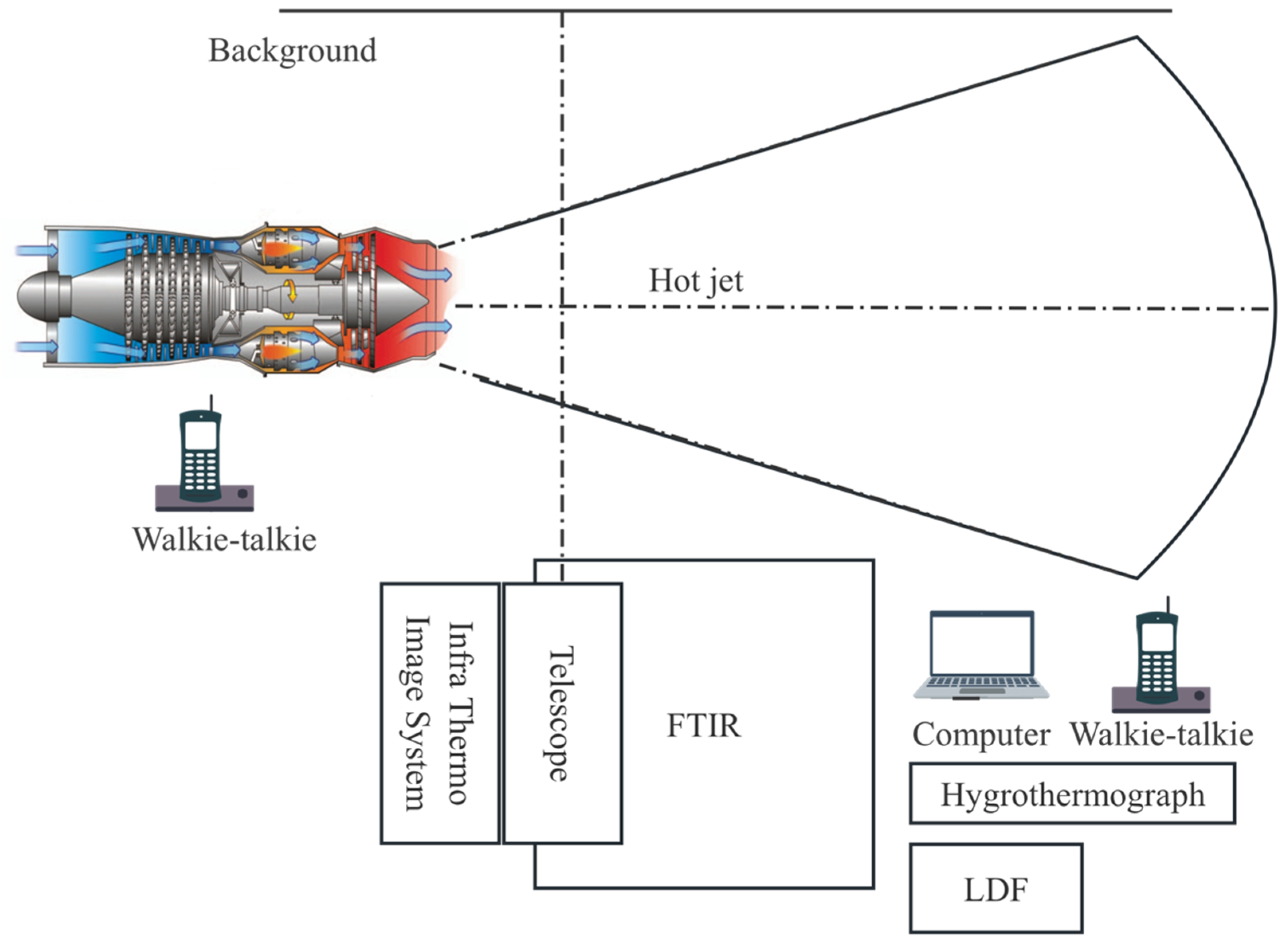
The study employs an outdoor experiment to gather infrared spectrum data on the hot jet from various types of aero-engines. Detailed specifications of the two telemetry FT-IR spectrometer devices utilized in the experiment are provided in

Table 1. Parameters for Fourier transform infrared spectrometers.

Name	Measurement Pattern	Spectral Resolution (cm−1)	Spectral Measurement Range (µm)	Full Field of View Angle
EM27	Active/Passive	Active: 0.5/1 Passive: 0.5/1/4	2.5~12	30 mrad (no telescope) (1.7°)
Telemetry Fourier Transform Infrared Spectrometer	Passive	1	2.5~12	1.5°

.

The experiment used two FT-IR spectrometers to measure the hot jet emitted from an aero-engine simultaneously. The spectrometers were positioned at a distance of five to ten meters from the aero-engine, allowing for measurement of the hot jet region of the aero-engine, ensuring that the hot jet energy filled the field of view and yielded high signal-to-noise ratio measurements. The layout of the experimental scene in the outfield is shown in Figure 3.

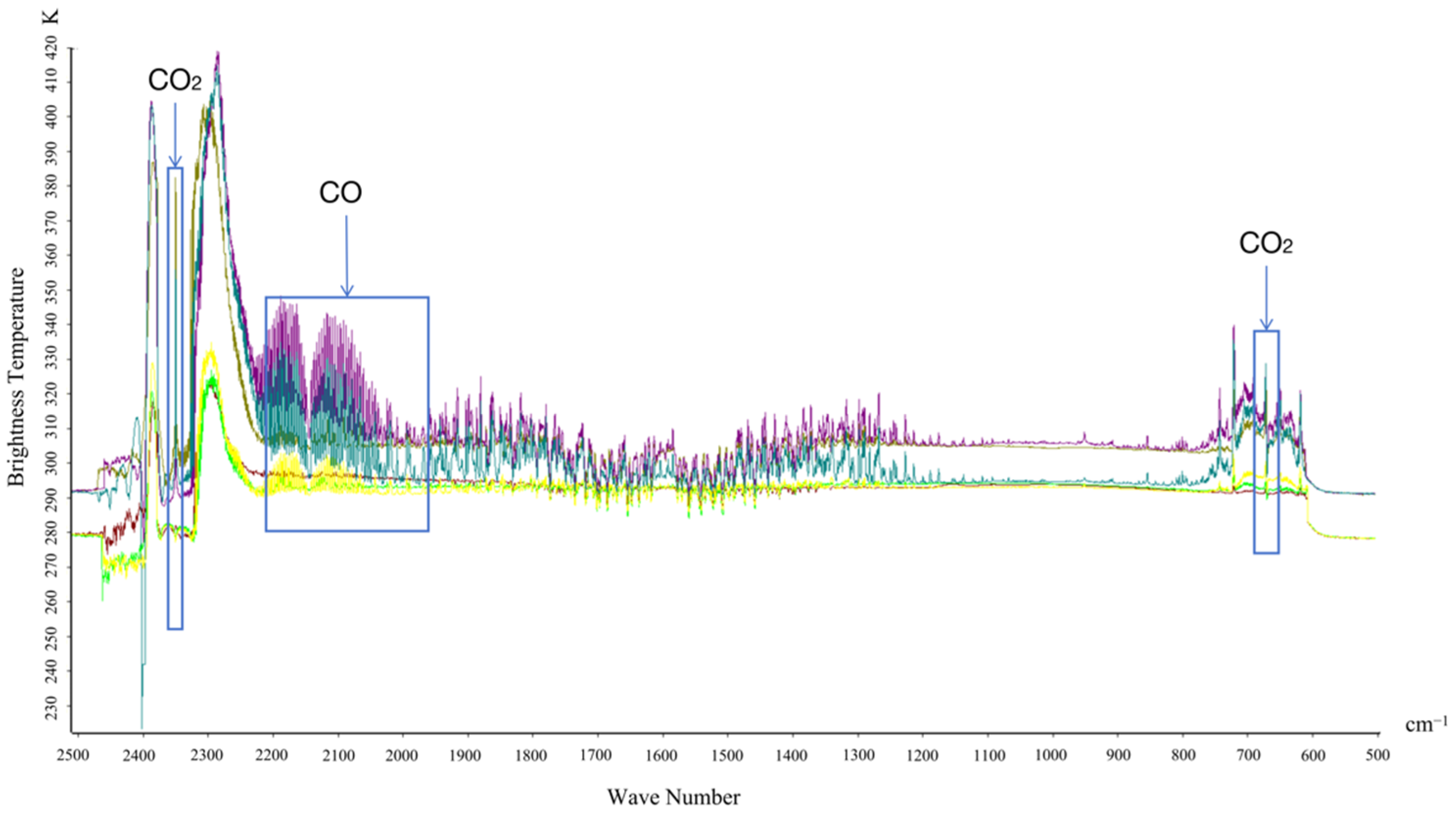
The bright temperature spectrum diagram of the six engine types obtained from the outdoor experiment is shown in Figure 4. The infrared characteristic peak positions of carbon monoxide and carbon dioxide emissions are highlighted and labeled in the graph, focusing on the distinct 660–2420 cm⁻¹ wavelength range.

This paper examines the peak values of three combustion byproducts, namely CO₂, H₂O, and CO. It is observed that the measured spectrum curve exhibits distinct and stable characteristic peaks at 2349 cm⁻¹ and 667 cm⁻¹ for the anti-symmetric stretching vibration and bending vibration of CO₂, respectively. These peaks are clearly visible in the spectral graph. Additionally, a characteristic peak at 2143 cm⁻¹ is formed due to the stretching vibration of the C≡O bond in CO; however, its intensity gradually weakens with increasing rotational speed. The characteristic band of water vapor does not exhibit prominence in the measured spectrum graph. Infrared spectra for common gases can be accessed from NIST and PCDL libraries. Based on the NIST library [21], we have compiled a list (

Table 2. Infrared characteristics of hot jet gas from aero-engines and molecular vibration modes.

Substance	Infrared Feature Location	Molecular Vibration Mode
Steam (H2O)	1600	Bending vibration
	3400	Symmetric stretching vibration
	3700	Asymmetric stretching vibration
Carbon monoxide (CO)	2150	Triple frequency vibration mode
Carbon dioxide (CO2)	667	Bending vibration
	2349	Asymmetric stretching vibration

) showcasing infrared spectral positions and molecular vibrations types specific to aero-engine jet gas.

Therefore, based on the reference of characteristic positions of CO₂ and CO in relation to measured spectral conditions, as well as the data requirements of CAE layers, the spectral range of 660–2420 cm⁻¹ was selected for feature extraction and classification experiments.

The data set of hot jet spectra of aero-engine collected from outdoor experiments is shown in

Table 3. A data set of hot jet spectra from six types of aero-engines.

Dataset	Type	Number of Data Pieces	Full Band Data Volume	Select Range Data Volume
1	Engine 1 (Turbojet)	193	16,384	832
2	Engine 2 (Turbojet)	48	16,384	832
3	Engine 3 (Turbojet)	199	16,384	832
4	Engine 4 (Turbofan)	775	16,384	832
5	Engine 5 (Turbofan)	256	16,384	832
6	Engine 6 (Turbojet)	380	16,384	832

:

The effective spectral data obtained from the field experiment comprises a total of 1851 records. Following the standard practice in deep learning, these data points are randomly sampled in an 8:1:1 ratio to generate a spectral training set, a spectral validation set, and a spectral test set. Subsequently, the analysis focuses on the spectral data ranging from 660–2420 cm⁻¹, where each spectrum consists of 3648 two-dimensional data points that serve as the input for feature extraction in this study.

3. Spectral Feature Extraction and Classification Network

Section 3 introduces a CAE feature extraction network for aero-engine hot jet spectra. It covers the overall network architecture design, the CAE network components, and the methods of network training and prediction.

3.1. Overall Network Architecture Design

The classic spectrum feature extraction method is to convert the data into a new feature space by projecting the data and retaining the identifying information. Methods include PCA, Independent Component Analysis (ICA), Linear Discriminant Analysis (LDA), and One-Dimensional Discrete Wavelet Transform (1D-DWT) [22]. Deep learning spectrum feature extraction methods mainly include supervised learning methods (1DCNN and RNN) and unsupervised learning methods (AE and PCA) [23].

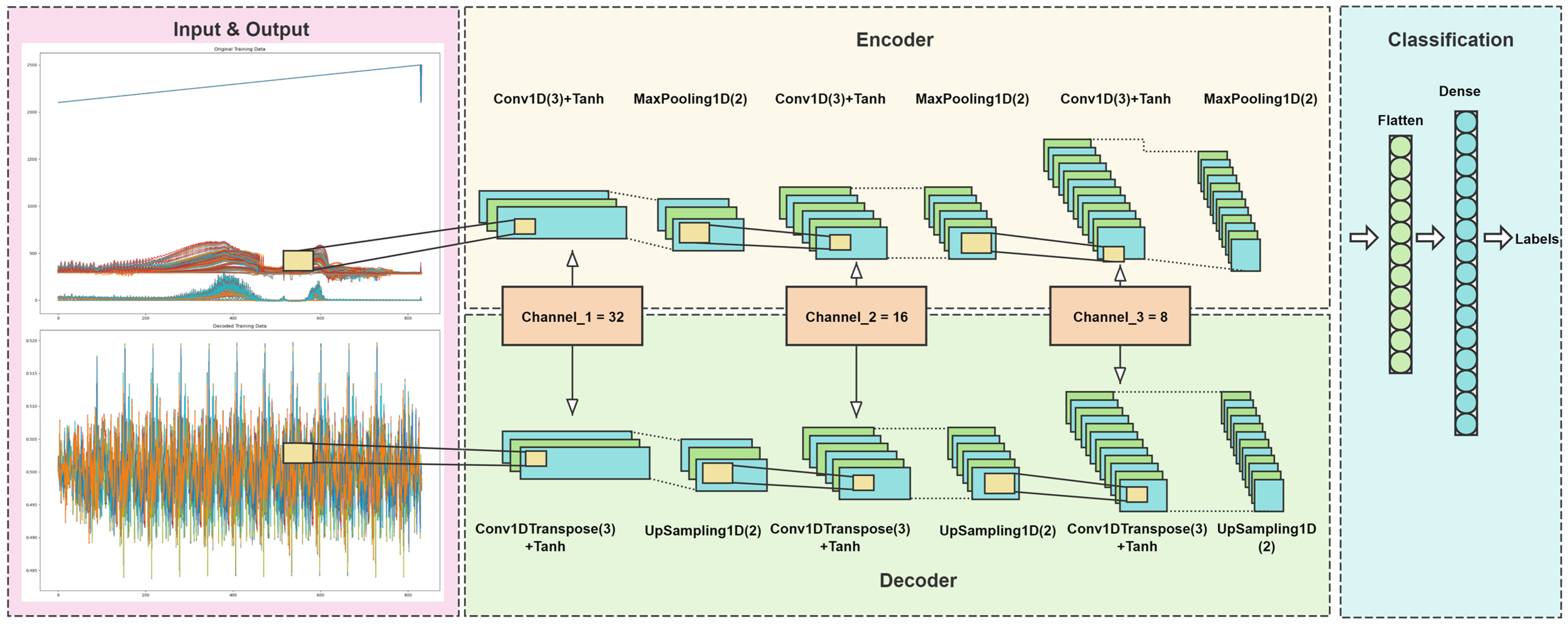
AE, a feature reduction technique in deep learning, comprises an encoder and a decoder. Through encoding, it acquires a low-dimensional representation of the input data and reconstructs the high-dimensional data using the decoded low-dimensional information. The structure of both the encoder and decoder in an AE is symmetrical. While shallow networks lack advantages in feature extraction, depth can significantly reduce function representation costs and training data requirements for learning functions. Hence, we employ a three-layer convolutional and max pooling structure (corresponding to three layers of deconvolution and up-sampling) to construct our base network for spec tral feature extraction and classification in our designed CAE, as depicted in Figure 5.

The CAE spectrum feature extraction and classification network consists of four modules: First, the input-output module is responsible for preprocessing spectral data by cropping the 660–2420 cm⁻¹ band as input to the network. Second, the encoding network comprises convolutional layers and max pooling layers. Convolutional layers are utilized to extract features and introduce nonlinearity through a Tanh activation function, while pooling layers reduce dimensionality of feature maps to decrease computational complexity. Third, the decoding network includes transpose convolutional layers and up-sampling layers. Up-sampling layers restore the original size of data, while transpose convolutions reconstruct data by performing inverse convolution operations to bring back features to their original scale. Lastly, the classification network consists of an expansion layer and a dense layer. The dense layer is employed for classification using softmax activation function that outputs class probabilities.

3.2. CAE Network Components

The paper improves the AE by designing a CAE spectrum feature extraction and classification network, which consists of convolution layers, max pooling layers, up-sampling layers, deconvolution layers, flattened layers, and dense layers.

(1) One-dimensional convolution layer (Cov1D): Convolution layers are the means by which CNNs extract features. Convolution layers perform linear and translation-invariant operations. Through convolution operations, we can extract features from data, which can enhance certain features of the original signal and reduce noise. The convolution between two functions can be defined as:

$$\left(f\times g\right)\left(x,y\right)={\sum }_i{\sum }_{j}f\left(i,j\right)\cdot g\left(x-i,y-j\right)$$

(2)

In this equation, $f$ denotes the spectrum data, $g$ represents the convolution kernel, $(x,y)$ signifies the output map position, and ($i,j$) indicates the position within the convolution kernel.

Convolution can be conceptualized as the superimposition of two functions with one being flipped and horizontally shifted. For a convolution layer, it can be expressed as follows:

$$\mathrm{Y}(\mathrm{x},\mathrm{y})=\mathrm{Activation}({\sum }_i{\sum }_{j}f(x\cdot stride+i,y\cdot stride+j)\cdot g(i,j)+b)$$

(3)

In the equation, $\mathrm{Y}$ represents the output feature map, $stride$ is the stride, $b$ is the bias term, and $\mathrm{Activation}$ is the activation function.

(2) Max pooling layer: Pooling is a down-sampling method in CNN that can reduce the data processing volume while retaining useful information. The convolution layer, pooling layer, and activation function layer can be understood as mapping the original data to the hidden feature space.

(3) Up-sampling layer: The up-sampling layer is used to increase the spatial resolution of the feature map.

(4) Convolution transpose layer: Also known as the deconvolution layer, it is used to perform up-sampling and feature map restoration. Its operation is similar to the inverse process of the convolution operation. The deconvolution layer can be represented as:

$$Y[i,j]={\sum }_m{\sum }_{n}X[i-m,j-n]\cdot K[m,n]$$

(4)

where $X$ represents the feature map, $Y$ represents the output feature map, $K$ represents the transposed convolution kernel, and $m$ and $n$ are the indices of the convolution kernel.

(5) Flattened layer: The flattened layer is used to concatenate multiple feature maps along the channel dimension. The resulting feature map contains all the channels from the input feature maps.

(6) Dense layer: Also known as a fully connected layer, it is used to convert the input feature map into a fixed-length output vector. Each output neuron is connected to all the input neurons. It is also used in CAE to combine Soft-max function for classification.

3.3. Network Training and Prediction Methods

(1) Optimizer: Adaptive learning rate optimization algorithms, including AdaGrad, RMSProp, Adam, and AdaDelta. Adaptive Moment Estimation (Adam) [24] estimates momentum and quadratic moments using exponentially weighted averages, with Adam’s state variables being:

$$\begin{array}{c}{\mathbf{v}}_t\leftarrow {\beta }_1{\mathbf{v}}_{t-1}+(1-{\beta }_1){\mathbf{g}}_t\\ {\mathbf{s}}_t\leftarrow {\beta }_2{\mathbf{s}}_{t-1}+(1-{\beta }_2){\mathbf{g}}_t^2\end{array}$$

(5)

where ${\beta }_1$ and ${\beta }_2$ are non-negative weighted parameters, usually set to ${\beta }_1$ = 0.9 and ${\beta }_2$ = 0.999. The standardized state variables can be obtained from the following equation:

$${\hat{\mathbf{v}}}_t={\displaystyle \frac{{\mathbf{v}}_t}{1-{\beta }_1^t}}$$

(6)

$${\hat{\mathbf{s}}}_t={\displaystyle \frac{{\mathbf{s}}_t}{1-{\beta }_2^t}}$$

(7)

The update formula for the gradient is obtained as follows:

$${\mathbf{g}}_t^{\prime }={\displaystyle \frac{\eta {\hat{\mathbf{v}}}_t}{\sqrt{{\hat{\mathbf{s}}}_t}+ϵ}}$$

(8)

where $\eta$ is the learning rate and $ϵ$ is a constant, which is usually set to 10⁻⁶. At the same time, the status update can be represented as:

$${\mathbf{x}}_t\leftarrow {\mathbf{x}}_{t-1}-{\mathbf{g}}_t^{\prime }$$

(9)

Adam optimizer dynamically adjusts the learning rate for each parameter, striking an optimal balance between computational complexity and performance by achieving low computational complexity while maintaining high performance.

(2) Loss function: the loss function consists of training loss and classification loss. The training loss uses the mean squared error ($MSE$) loss function, and the classification loss uses the sparse categorical cross entropy loss function. Two loss functions are set to contribute 50% each to the training.

The training loss $MSE$ can be expressed as:

$${\mathrm{Loss}}_{MSE}={\displaystyle \frac{1}{m}}{\sum }_{i=1}^m(y_i-{\hat{y}}_i)$$

(10)

In this equation, $m$ denotes the sample size, $y_i$ denotes the true value, and ${\hat{y}}_i$ denotes the predicted value. In the CAE, the loss function is utilized to compute the discrepancy between the input spectrum data and the reconstructed data, with the true value representing the spectrum data and the predicted value representing the reconstructed data.

Classification tasks often use the cross-entropy loss function, which is used to describe the difference in sample probability distributions and measure the difference between the distribution learned by the model and the true distribution. The cross-entropy loss function can be expressed as:

$${\mathrm{Loss}}_{cross entropy}=-{\displaystyle \frac{1}{N}}{\sum }_{i=0}^{N-1}{\sum }_{k=0}^{K-1}{y}_{i,k}\mathrm{l}\mathrm{n}{p}_{i,k}$$

(11)

In this equation, $y_{i,k}$ represents the true label of the $i$-th spectrum sample as $k$, with a total of $K$ label values and $N$ samples. Meanwhile, $p_{i,k}$ represents the probability that the $i$-th spectrum sample is predicted to be the $k$-th label value. The smaller the value of cross-entropy, the better the model’s predictive effect. In the CAE, the true label is the six types of aero-engine identification numbers (Class 0–5), and the samples are the dataset size.

(3) Activation function: the activation function in the convolution layer is the hyperbolic tangent function (Tanh). Tanh is a commonly used activation function that maps input values to continuous values within the range of −1 to 1. It can be expressed as:

$$\mathrm{T}\mathrm{a}\mathrm{n}\mathrm{h}(x)={\displaystyle \frac{e^x-e^{-x}}{e^x{+e}^{-x}}}$$

(12)

In this equation, $x$ represents the input value of a certain neuron in the neural network, which is the sum of the product of the neuron’s weight and the input, plus the bias term. The Tanh function has 0 as its symmetry center, converges quickly, improves the efficiency of weight updating, and alleviates the occurrence of gradient explosion.

(4) L2 regularization: L2 regularization is a method to prevent overfitting in models. The introduction of L2 regularization (weight decay) in convolutional layers aims to prevent model overfitting by limiting the size of weights, reducing excessive fitting to training data, and improving the generalization ability of the model towards unseen data. At the same time, L2 regularization encourages weights to be smaller but not completely zero, providing a smoothing effect that helps stabilize the model when facing new data. The L2 regularization term, denoted as $L_{\mathrm{total}}^{\prime }$, can be expressed as:

$$L_{\mathrm{total}}^{\prime }=w_1\cdot L_1+w_2\cdot L_2+\lambda {\sum }_i{w}_i^2$$

(13)

Among them, $L_1$ is the MSE loss function, $w_1$ is the weight of the loss function $L_1$, $L_2$ is the cross-entropy loss function, $w_2$ is the weight of the loss function $L_2$, λ represents regularization strength (usually set to 0.01), and $w_i$ represents the weights of convolutional layers.

4. Experiment Results and Analysis

Section 4 conducts an experiment on the infrared spectrum dataset of the aero-engine hot jet and analyzes the experiment results, including the experiment results and analysis of the CAE method and the comparison algorithms.

4.1. Experimental Results and Analysis of CAE

To assess the effectiveness of the CAE presented in this paper, computational experiments are carried out on a Windows 10 workstation (MSI Technology, Shanghai, China) with 32 GB of RAM, featuring an Intel Core i7-8750H processor and a GeForce RTX 2070 graphics card.

The performance measures for classifying aero-engine hot jet infrared spectra encompass Accuracy, Precision, Recall, F1-score, Confusion Matrix, ROC curve, and AUC value. Among these metrics, Accuracy is suitable for evaluating classification under balanced category distribution, while Precision is appropriate for assessing classification under balanced category distribution. Recall signifies the model’s capacity to capture positive samples and is applicable in scenarios where reducing false negatives is crucial. The F1-score is pertinent when balancing precision and recall becomes essential. The Confusion Matrix illustrates the comparison between the model’s predictions and true labels. The ROC curve offers a clear visual depiction of the model’s performance across all possible threshold values, where proximity to the upper left corner indicates superior overall performance by the model. The AUC value gauges the overall classification performance of the model and serves as an assessment tool under imbalanced category distribution. These metrics establish a standardized framework for comparing different models used in infrared spectrum classification; comprehensive evaluation enables selection of an optimal infrared spectrum classification model.

The specific parameters of the CAE spectrum feature extraction and classification network are given in

Table 4. CAE spectrum feature extraction and classification network parameter information.

Methods	Parameter Settings
CAE	Hidden layer: CHANNEL_1 = 32, CHANNEL_2 = 16 CHANNEL_3 = 8, CHANNEL_OUTPUT = 1
	Encoded: (CHANNEL_1 to CHANNEL_3) Conv1D (kernel_size = 3, activation = ‘Tanh’, padding = ‘same’, kernel_regularizer = l2(0.01)) MaxPooling1D (2, padding = ‘same’)
	Decoded: (CHANNEL_3 to CHANNEL_1) Conv1DTranspose (kernel_size = 3, strides = 1, activation = ‘Tanh’, padding = ‘same’) UpSampling1D(2)
	Classification: Flatten = Flatten() Dense (num_classes, activation = ‘softmax’)
	Train: optimizer = tf.keras.optimizers.Adam (learning rate = 0.0001) loss = [‘mse’, ‘sparse_categorical_crossentropy’], loss_weights = [0.5, 0.5] metrics = [‘accuracy’] epochs = 500 batch size = 64

:

The detailed shape parameters and number of parameters are shown in

Table 5. CAE spectrum feature extraction and classification network model structure parameter.

Model	Total Params: 26,424 Trainable Params: 26,424
Layer (type)	Output Shape	Param
data_input (InputLayer)	(3648, 2)	0
conv1d (Conv1D)	(3648, 32)	224
max_pooling1d (MaxPooling1D)	(1824, 32)	0
conv1d_1 (Conv1D)	(1824, 16)	1552
max_pooling1d_1 (MaxPooling1D)	(912, 16)	0
conv1d_2 (Conv1D)	(912, 8)	392
(Encoded) max_pooling1d_2 (MaxPooling1D)	(456, 8)	0
up_sampling1d (UpSampling1D)	(912, 8)	0
conv1d_transpose (Conv1DTranspose)	(912, 8)	200
up_sampling1d_1 (UpSampling1D)	(1824, 8)	0
conv1d_transpose_1 (Conv1DTranspose)	(1824, 16)	400
up_sampling1d_2 (UpSampling1D)	(3648, 16)	0
conv1d_transpose_2 (Conv1DTranspose)	(3648, 32)	1568
(Dncoded) conv1d_3 (Conv1D)	(3648, 2)	194
flatten (Flatten)	3648	0
dense (Dense)	6	21,894

:

According to the parameters in the table, 500 training experiments were conducted on the training and validation set of the spectrum dataset, and the change curve of the loss function and accuracy was obtained as Figure 6:

From the loss function, it can be seen that the model has been effectively trained in 500 epochs and that the loss function has gradually become proficient. The accuracy curve shows that the model has reached 90% correct classification after 250 epochs.

We selected the model with the lowest loss value as the best model for the experiment and used this model to conduct classification prediction experiments on the prediction set data. The experiment results were evaluated and obtained and are shown in

Table 6. Experiment results of CAE spectrum feature extraction and classification network spectral classification.

	Evaluation Criterion	Accuracy	Precision Score	Recall	Confusion Matrix	F1-Score	Running Time
Method
CAE		96.09%	98.72%	94.70%	[17  0  0   0  0   0] [0   7  0   0  0   0] [0   0  16  0  0   0] [0   0  0  84  0   0] [0   0  0   7  15  0] [0   0  0   0  0  33]	96.18%	1.5718 s

:

CAE performs well in terms of accuracy, precision, recall, and F1-score. Overall, 96.09% of the samples were correctly classified. A 98.72% precision means that the model is almost always correct when predicting categories, and 94.70% recall indicates that the model can recognize most positive samples but that there are still a small number of positive samples that have not been recognized. A 96.18% F1-score indicates that the model still performs well when dealing with class imbalance.

Using the experimental results, the confusion matrix and ROC curve of the CAE spectrum feature extraction and classification network were determined, as shown in Figure 7:

According to the analysis of the diagonal elements of the confusion matrix, categories 0, 1, 2, 3, and 5 were correctly predicted, while there were 7 cases of misclassification of category 3 in category 4, indicating difficulties in identifying category 4. The running time is 3.5753 s, indicating that the model also performs well in terms of efficiency. Further optimization of the model or adding more data for training can be considered to alleviate this. The running time is also within an acceptable range and is suitable for practical applications.

The ideal ROC curve will closely follow the top left corner (0, 1), which means that the model can perfectly distinguish between positive and negative cases in all cases. The green and dark blue curves in the figure indicate that there is misclassification between category 3 and category 4, while the other categories achieve correct classification. The AUC table obtained from the ROC chart is shown in

Table 7. AUC value results of CAE spectrum feature extraction and classification network.

AUC	Class 0	Class 1	Class 2	Class 3	Class 4	Class 5
CAE	1.00	1.00	1.00	0.96	0.84	1.00

:

The range of AUC values is 0 to 1, and the closer the value is to 1, the better the classification performance of the model. Overall, the classification performance of the model is very good in most categories. In Class 3, the classification performance of the model is also very high, but there are some small errors. In Class 4, the classification performance of the model is relatively weak and needs further optimization and adjustment to improve classification accuracy.

In summary, the CAE network shows excellent performance in the task of classifying aero-engines and has the potential for classification and recognition.

4.2. Comparison Algorithm Results and Analysis

4.2.1. Different Optimizers and Activation Functions in CAE Networks

(1) Different optimizers

The choice of an optimizer is a key point in network training. The CAE structure in Table 4 was tested on the dataset using different optimizers (SGD, SGDM, Adagrad, and RMSProp); the results are shown in

Table 8. Results of experiments with different optimizers.

Optimizers	Prediction Accuracy	Training Time/s	Prediction Time/s
SGD	37%	1340.58	1.04
SGDM	38%	1339.85	0.79
Adagrad	57%	1336.83	0.72
RMSProp	92%	1378.75	0.83
Adam	92%	1347.26	0.78

and Figure 8:

From Table 8, it can be seen that RMSProp and Adam not only provide the highest prediction accuracy, but also have relatively shorter prediction times, making them suitable for applications that require high accuracy. In contrast, the difference in training and prediction times among the five optimizers is not significant. From the curves of Loss and Accuracy, it can be seen that the convergence of SGD, SGDM, and Adagrad is poor, which may indicate that the model training has fallen into a local minimum.

Comparing the classification results with the curves of Loss and Accuracy can show that the Adam optimizer can converge very quickly and has a high classification accuracy.

(2) Different activation functions

The activation function determines the output of the neuron and the overall learning ability of the network. We conducted experiments on the CAE with the Table 4 structure using different activation functions such as ReLU, Tanh, Sigmoid, ELU, and LeakyReLU; the obtained results are shown in

Table 9. Results of experiments with different activation functions.

Optimizers	Prediction Accuracy	Training Time/s	Prediction Time/s
ReLU	94%	1174.17	1.16
Tanh	94%	1170.31	0.76
Sigmoid	69%	1164.32	0.7
ELU	94%	1159.69	0.75
LeakyReLU	92%	1150.72	0.77

and Figure 9:

Activation functions ReLU, Tanh, and ELU perform best in terms of accuracy and are suitable for tasks with high requirements for prediction accuracy.

4.2.2. Traditional Feature Extraction and Classifier Algorithms

PCA [25,26] is used to extract the most relevant features from high-dimensional data and project the original data into a new low dimensional space through linear transformation to maximize the variance of the projected data. Using dimensionality reduction, the complexity of the data can be reduced, the calculation of the model can be simplified, and the information of the original data can be preserved as much as possible. The process of using PCA for spectral feature extraction can be represented as:

(1) Centralization: subtracting the mean of each feature from the original data to make the mean of the data zero:

$${\mathbf{X}}_{\mathrm{c}\mathrm{e}\mathrm{n}\mathrm{t}\mathrm{e}\mathrm{r}\mathrm{e}\mathrm{d}}=\mathbf{X}-\mathsf{\mu }$$

(14)

where ${\mathbf{X}}_{\mathrm{c}\mathrm{e}\mathrm{n}\mathrm{t}\mathrm{e}\mathrm{r}\mathrm{e}\mathrm{d}}$ stands for centralized spectrum data, $X$ stands for spectrum data, and $\mu$ stands for the mean value.

(2) Calculate covariance matrix: perform covariance analysis on the data and calculate the covariance between features:

$$\mathrm{C}\mathrm{o}\mathrm{v}\mathrm{a}\mathrm{r}\mathrm{i}\mathrm{a}\mathrm{n}\mathrm{c}\mathrm{e} \mathrm{m}\mathrm{a}\mathrm{t}\mathrm{r}\mathrm{i}\mathrm{x}={\displaystyle \frac{1}{\mathrm{n}-1}}{{\mathbf{X}}_{\mathrm{c}\mathrm{e}\mathrm{n}\mathrm{t}\mathrm{e}\mathrm{r}\mathrm{e}\mathrm{d}}}^{\mathrm{T}}{\mathbf{X}}_{\mathrm{c}\mathrm{e}\mathrm{n}\mathrm{t}\mathrm{e}\mathrm{r}\mathrm{e}\mathrm{d}}$$

(15)

where $n$ represents the number of spectrum data and ${{\mathbf{X}}_{\mathrm{c}\mathrm{e}\mathrm{n}\mathrm{t}\mathrm{e}\mathrm{r}\mathrm{e}\mathrm{d}}}^{\mathrm{T}}$ represents the transpose of the ${\mathbf{X}}_{\mathrm{c}\mathrm{e}\mathrm{n}\mathrm{t}\mathrm{e}\mathrm{r}\mathrm{e}\mathrm{d}}$ matrix.

(3) Solving the feature space: perform feature value decomposition on the covariance matrix to obtain feature values and corresponding feature vectors.

$$\mathbf{C}=\mathbf{V}\mathsf{\Lambda }{\mathbf{V}}^{\mathrm{T}}$$

(16)

where $\mathbf{V}$ is the feature vector matrix and $\mathsf{\Lambda }$ is the diagonal matrix with feature values on the diagonal. Select the feature vectors corresponding to the first (k) largest feature values to form the matrix ${\mathbf{V}}_k$.

(4) For data dimensionality reduction: $Z$ is the reduced matrix, with each row corresponding to a sample and each column corresponding to a principal component:

$$\mathbf{Z}={\mathbf{X}}_{\mathrm{c}\mathrm{e}\mathrm{n}\mathrm{t}\mathrm{e}\mathrm{r}\mathrm{e}\mathrm{d}}{\mathbf{V}}_{\mathrm{k}}$$

(17)

Through these steps, PCA transforms the original data $X$ into a new feature space $Z$, achieving feature extraction and data dimensionality reduction. PCA features need to be combined with classifier methods to complete the task of spectral classification.

To verify the effectiveness of PCA features, we selected data from the same frequency band and used PCA to extract features. We combined representative classifier algorithms SVM [27], XGBoost [28], AdaBoost [29], and Random Forest [30] to conduct classification experiments on the infrared spectra of aero-engine hot jets.

Table 10. Table of parameters for classifier methods.

Methods	Parameter Settings
SVM	decision_function_shape = ‘ovr’, kernel = ‘rbf’, max_iter = 100, tol = 1 × 10−3
XGBoost	objective = ‘multi:softmax’, n_estimators = 100
Adaboost	n_estimators = 100
Random Forest	n_estimators = 100

provides the parameter settings for the classification algorithm:

This paper conducted a comparative experiment by combining PCA features and classifiers using the same band data, and obtained the classification results shown in

Table 11. Experiment results of spectrum classification using PCA feature classifier.

	Evaluation Criterion	Accuracy	Precision Score	Recall	Confusion Matrix	F1-Score	Running Time
Method
PCA + SVM		73.18%	53.59%	57.38%	[5  0  12  0   0  0] [0  0  0   0   2  5] [3  0  6   5   2  0] [0  0  0  65  16  3] [0  0  0   0  22  0] [0  0  0   0   0 33]	52.94%	0.7325 s
PCA + XGBoost		73.18%	53.59%	57.38%	[5  0  12  0  0   0] [0  0  0  0   2   5] [3  0  6  5   2   0] [0  0  0  65  16  3] [0  0  0  0  22   0] [0  0  0  0   0  33]	52.94%	7.0440 s
PCA + Adaboost		43.02	43.32	37.77	[0   0  0   0  0  17] [0   3  4   0  0   0] [0   0  16  0  0   0] [0   0  0  50  0  34] [0   0  0  11  0  11] [13  0  0  12  0   8]	38.02%	17.0578 s
PCA + Random Forest		99.44%	99.80%	98.95%	[17  0  0   0  0   0] [0   7  0   0  0   0] [0   0  15  1  0   0] [0   0  0  84  0   0] [0   0  0   0  22  0] [0   0  0   0  0  33]	99.36%	2.1833 s

:

The results of PCA classification analysis show that the performance of SVM and XGBoost is very similar, with an accuracy rate of 73.18% and F1-score of 52.94%, but the running time of XGBoost is significantly longer. The performance of AdaBoost is poor, with an accuracy rate of only 43.02%, F1-score of 38.02%, and the longest running time. Random Forest performs best, with an accuracy rate of 99.44% and F1-score of 99.36%, and a relatively shorter running time. From the confusion matrix analysis, the classification performance of SVM and XGBoost is the same, and the classifiers have large errors in predicting Class 0 and Class 1, while the performance in Classes 3, 4, and 5 is good. The overall performance of the AdaBoost classifier is poor, especially the misclassification of Class 0 and Class 5, while the performance in Classes 2 and 3 is better. The overall performance of Random Forest is the best, with high accuracy rates for almost all classes and fewer misclassifications. Combining PCA features and the classifier’s classification results, PCA features and Random Forest have outstanding performance in terms of classification accuracy and running efficiency when performing spectrum classification tasks. To compare the contribution of PCA features and CAE features to classification, we conducted experiments by combining CAE features with the same classifier, and the experimental results are shown in

Table 12. Experiment results of spectrum classification using CAE feature classifier.

Evaluation Criterion Method	Accuracy	Precision Score	Recall	Confusion Matrix	F1-Score	Running Time
CAE + SVM	79.89%	89.66%	92.55%	[17  0  0   0   0  0] [0   7  0   0   0  0] [0   0  16  0   0  0] [0   0  0  49  35  0] [0   0  0   0  22  0] [0   0  0   0  1  32]	87.85%	0.3261 s
CAE + XGBoost	79.89%	89.65%	92.55%	[17  0  0   0  0   0] [0   7  0   0  0   0] [0   0  16  0  0   0] [0   0  0  49  35  0] [0   0  0   0  22  0] [0   0  0   0  1  32]	87.86%	2.2100 s
CAE + Adaboost	61.45%	41.31%	46.43%	[0  0  17  0   0   0] [0  0   7  0   0   0] [0  0  16  0   0   0] [0  0  0  66  18   0] [0  0  0  12  10   0] [0  0  0   0  15  18]	40.00%	4.3493 s
CAE + Random Forest	96.65%	98.89%	95.45%	[17  0   0  0   0   0] [0   7   0  0   0   0] [0   0  16  0   0   0] [0   0   0  84  0   0] [0   0   0  6  16   0] [0   0   0  0   0  33]	96.79%	1.2437 s

:

Although the CAE has already shown a 96% accuracy rate in network prediction, the classification experiment results of comparing PCA features with CAE features show that when CAE is used as a feature extraction method combined with a classifier for classification tasks, SVM, XGBoost, Adaboost classifiers outperform PCA, with significantly higher accuracy and F1-score. In the same feature extraction method, the Random Forest classifier performs best in both tables and is more suitable for our spectral features, achieving accurate classification results. Comprehensively considering CAE’s classification performance for each category in the confusion matrix, the misclassification between categories 3 and 4 indicates that CAE features are lacking when trying to distinguish between categories 3 and 4, while other categories can achieve very high classification results. In most cases, the CAE method has a shorter running time, especially when combined with the SVM classifier, with CAE’s running time far lower than PCA.

Overall, the CAE features have better performance in spectrum classification than PCA features, especially in terms of precision, recall, and F1-score. In addition, the running time of CAE prediction is shorter, which will lead to greater efficiency in actual applications.

4.2.3. Deep Learning Classification Algorithm

To evaluate the performance of our designed CAE within deep learning methodologies, we developed three variants of autoencoders, AE, CSAE, and CVAE, for comparative analysis.

The CSAE and CVAE are both variant models based on CAE. Specifically, CSAE incorporates L1 regularization as a sparsity constraint within the encoder, while also integrating a sparse regularization term into the loss function. This approach enhances the model’s capacity to compress input features and improves its robustness against noise through enforced sparsity. In contrast, CVAE leverages concepts from VAE by employing a probabilistic framework for encoding, enabling the model to conduct probabilistic modeling and effectively learn the distribution characteristics of the input data.

We conducted a comparative experimental study on deep learning classification methods utilizing an identical wavelength range (660–2420 cm⁻¹), along with consistent parameters such as layer structure for AE, batch size, learning rate, optimizer settings, and epochs as outlined in Table 4. The key parameters for these models are detailed in

Table 13. Spectral feature extraction algorithm and the classification comparison networks parameter information.

Methods	Parameter Settings
AE	CHANNEL_1 = 32, CHANNEL_2 = 16 CHANNEL_3 = 8, CHANNEL_OUTPUT = 1 Encoded: (CHANNEL_1 to CHANNEL_3) Flatten = Flatten() Dense (CHANNEL activation = ‘Tanh’) Decoded: (CHANNEL_2 to CHANNEL_1) Dense (CHANNEL, activation = ‘Tanh’) Dense (np.prod (input_shape_data), activation = ‘sigmoid’) Classification: Dense (num_classes, activation = ‘softmax’) optimizer = tf.keras.optimizers.Adam (lr = 0.0001) loss = [‘mse’, ‘sparse_categorical_crossentropy’], loss_weights = [0.5, 0.5] metrics = [‘accuracy’] epochs = 500 batch size = 64
CSAE	CHANNEL_1 = 32, CHANNEL_2 = 16 CHANNEL_3 = 8, CHANNEL_OUTPUT = 1 Encoded: (CHANNEL_1 to CHANNEL_3) Conv1D (kernel_size = 3, activation = ‘Tanh’, padding = ‘same’, kernel_regularizer = l1(0.01)) MaxPooling1D (2, padding = ‘same’) Decoded: (CHANNEL_3 to CHANNEL_1) Conv1DTranspose (kernel_size = 3, strides = 1, activation = ‘Tanh’, padding = ‘same’) UpSampling1D(2) Flatten = Flatten() Dense (num_classes, activation = ‘softmax’) optimizer = tf.keras.optimizers.Adam (lr = 0.0001) reconstruction_loss = K.binary_crossentropy (x_true, x_pred) sparsity_loss = K.mean(K.square(K.sum(x_pred, axis = (1, 2))− alpha)) loss = [sparse_coding_loss(alpha), ‘categorical_crossentropy’], loss_weights = [0.5, 0.5] metrics = [‘accuracy’] epochs = 500 batch size = 64
CVAE	CHANNEL_1 = 32, CHANNEL_2 = 16 CHANNEL_3 = 8, CHANNEL_OUTPUT = 1 Encoded: (CHANNEL_1 to CHANNEL_3) Conv1D (kernel_size = 3, activation = ‘Tanh’, padding = ‘same’, kernel_regularizer = l2(0.01)) MaxPooling1D (2, padding = ‘same’) Latent space: Dense (z_mean) Dense (z_log_var) Lambda (z = z_mean + tf.exp(0.5 × z_log_var) × epsilon) Decoded: (CHANNEL_3 to CHANNEL_1) Conv1DTranspose (kernel_size = 3, strides = 1, activation = ‘Tanh’, padding = ‘same’) UpSampling1D(2) Flatten = Flatten() Dense (num_classes, activation = ‘softmax’) optimizer = tf.keras.optimizers.Adam (lr = 0.0001) loss = [‘mse’, ‘sparse_categorical_crossentropy’], loss_weights = [0.5, 0.5] metrics = [‘accuracy’] epochs = 500 batch size = 64

.

We conducted spectral classification experiments using deep learning methods based on the model information provided in the parameter table and obtained evaluation results as presented in

Table 14. Experiment results of spectrum classification using spectral feature extraction algorithm and the classification comparison networks.

	Evaluation Criterion	Accuracy	Precision Score	Recall	Confusion Matrix	F1-Score	Running Time/s
Method
AE		46.92%	7.82%	16.67%	[0  0  0  17  0  0] [0  0  0  7   0  0] [0  0  0  16  0  0] [0  0  0  84  0  0] [0  0  0  22  0  0] [0  0  0  33  0  0]	10.65%	0.4111
CSAE		94.41%	96.81%	93.26%	[17  0  0   0   0  0] [0   7  0   0   0  0] [1   0  15  0   0  0] [0   0  0  82   0  2] [0   0  0  7   15  0] [0   0  0  0   0  33]	94.47%	1.6997
CVAE		88.83%	92.16%	84.96%	[17  0  0   0  0   0] [1   5  1   0  0   0] [0   0  16  0  0   0] [0   0  0  78  1   5] [0   0  0  12  10  0] [0   0  0   0  0  33]	86.78%	1.2863

and

Table 15. AUC value results of spectral feature extraction algorithm and the classification comparison networks.

AUC	Class 0	Class 1	Class 2	Class 3	Class 4	Class 5
AE	0.50	0.50	0.50	0.50	0.50	0.50
CSAE	1.00	1.00	0.97	0.95	0.84	0.99
CVAE	1.00	0.86	1.00	0.90	0.72	0.98

and Figure 10 and Figure 11.

Based on the analysis of AE, it is evident that its classification accuracy is merely 46.92% under identical parameter conditions. This indicates an insufficient acquisition of discriminative features necessary for successful classification. Despite exhibiting the highest computational efficiency, most categories remain misclassified. Conversely, CSAE achieves an impressive accuracy rate of 94.41%, and surpassing 90% in all other performance metrics. These results demonstrate accurate classification across most samples, particularly in class 0, class 1, and class 5 where CSAE performs exceptionally well. However, some misclassifications are observed in class 2 and class 3, while the majority occur within class 4. Although CSAE’s runtime slightly exceeds that of AE’s, it still maintains acceptable efficiency levels. CVAE attains an accuracy rate of 88.83%. The confusion matrix reveals complete correct classifications for classes 0, 2, and 5; only a few misclassifications are present in classes 1 and 3. Despite this, a significant issue arises with misclassification between class four and three where a considerable number of samples are erroneously assigned.

Simultaneously, the spectral data set was utilized to assess the performance of AE, CSAE, and CVAE models, with their corresponding AUC values presented in Table 13 for reference.

The AUC for the AE was 0.50, indicating that the current network architecture did not effectively learn the classification features. In contrast, both CSAE and CVAE exhibited strong performance, with AUC values approaching 1. CSAE outperformed both CVAE and AE across most categories, particularly excelling in Class 0, Class 1, and Class 5. While CVAE demonstrated superior performance compared to AE in certain categories, it showed suboptimal results in Class 4.

The proposed CAE in this study is a superior choice for classifying hot jet spectra of aero-engines, achieving a remarkable classification accuracy of 96% and a prediction precision of 1.57 s. However, the current spectral data set used in this research has certain limitations, including a restricted range of aero-engine models and imbalanced data distribution among different models. Therefore, future investigations will focus on establishing a more comprehensive spectral dataset.

The establishment of the dataset for hot jet spectra in aero-engines is still in its infancy. The resolution and composition of the data differ greatly from HSIs, which also poses more requirements for parameter research in paper models. Increasing the width of the hidden layer can accelerate the convergence speed of the model, enabling it to quickly achieve better classification accuracy but significantly increasing training parameters and time. Smaller network models have relatively slower convergence speeds during training but can also achieve good accuracy within a shorter time frame with the same number of epochs. Finding a balance between network parameters, training time, and memory consumption is a challenging aspect of research. Additionally, addressing CNN’s weakness in global feature extraction would be an excellent direction for improvement. Currently, successful applications of Transformer models on HSI data will become new avenues for exploration in papers. Combining Transformer models with current spectral datasets to achieve higher classification accuracy will present opportunities and challenges for new attempts.

5. Conclusions

In response to the classification problem of aero-engines in aero-engine failure detection, this study employs telemetry FT-IR spectrometers to measure the infrared spectra of hot jets for six types of aero-engines. A CAE spectral classification network is designed, achieving an impressive accuracy rate of 96% and a rapid classification speed of 1.57 s for aero-engine classification, thereby meeting the real-time prediction requirements of aero-engines. The specific contributions made in this paper are as follows: (1) Utilizing telemetry FT-IR spectrometers to measure the infrared spectral data from hot jets emitted by aero-engines and establishing a comprehensive data set for these six types of hot jet. By analyzing CO₂ and CO composition components within these plumes, we determine that the wavelength range from 660–2420 cm⁻¹ exhibits distinct classification features suitable for input into our classification network. (2) We propose a CAE network for spectral classification based on an AE combined with CNNs. The encoder network comprises convolutional layers and max pooling layers, while the decoder network consists of up-sampling layers and deconvolutional layers. Additionally, a flattened layer and a dense layer are incorporated into the classifier network. (3) Classic PCA combined with various classifiers such as SVM, XGBoost, AdaBoost, and Random Forest, along with AE and their variants CSAE and CVAE, are applied to classify our dataset containing infrared spectra data obtained from aero-engine hot jets. Research on the spectral data of jet engine exhaust is rapidly advancing; however, the significant differences in data resolution and composition between it and HSI pose new application requirements for deep learning classification models. Following this paper, we will focus on expanding the dataset of hot jet spectral data and studying higher-precision classification models. Additionally, the CAE network can be integrated with a real-time health monitoring system for aero-engines. By collecting FT-IR spectral data from these engines, the network is capable of rapidly identifying faults. This paper will also undertake systematic research on the integration methodology in future work.