
Statistical Analysis of LEO and GEO Satellite Anomalies and Space Radiation

 , , and
Abstract
1. Introduction
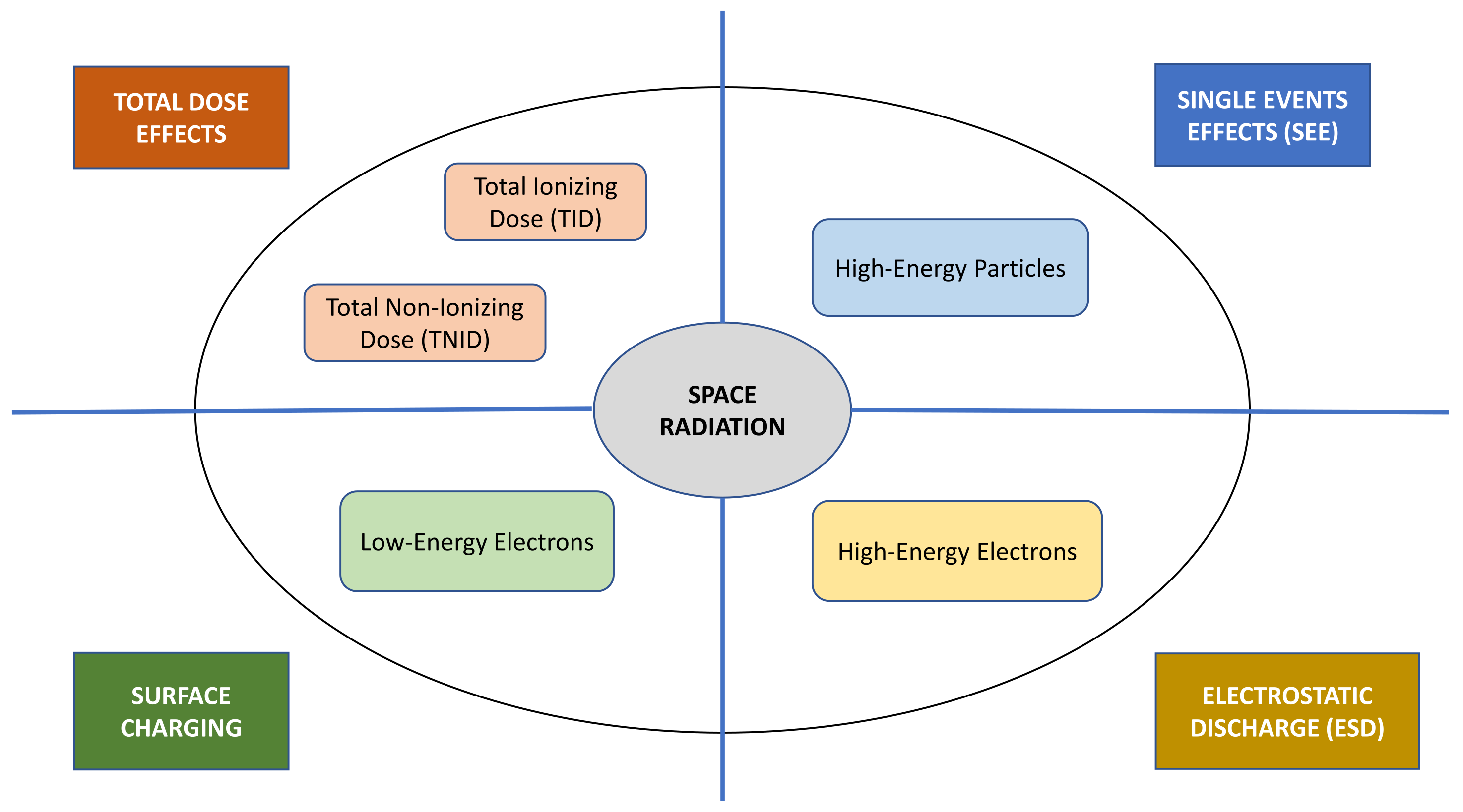
2. Space Weather Effects on Satellite Systems
- Surface charging of satellite: Caused by low-energy electrons (<100 keV), observed typically in the inner magnetosphere during geomagnetic storms [12].
- Satellite internal electrostatic discharge: Caused by high-energy electrons (>100 keV), observed in Earth’s dynamic outer radiation belt.
- Single event effects: Caused by high-energy protons (>10 MeV) and heavier ions, derived from solar flares, and coronal mass ejections (CMEs).
- Total dose effects: Caused by cumulative charged protons and electrons derived from several space weather events.
- Others: Other effects such as those related to communications and attitude control failures, due to magnetic field variations, and ionospheric anomalies, among others [31].
3. Data and Methods
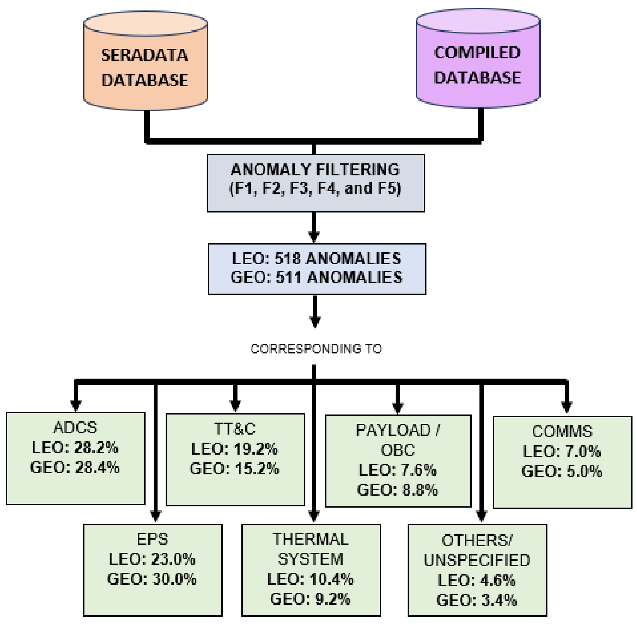
3.1. LEO and GEO Satellite Anomalies
- Anomalies lacking a clear specification of the month and day of occurrence in their description were discarded, given the significance of the anomalies’ date in the analysis.
- Launch failures were removed as their occurrence is typically attributed to mechanical or procedural errors unrelated to space radiation.
- Unless the cause of the specified anomaly is closely related to radiation effects (e.g., ESD), failures occurring within the first month after launch were excluded, as they may be due to “infancy failures” [41] or lack of testing processes.
- Anomalies whose cause is not exclusively attributable to radiation effects are discarded. Clear examples are those anomalies related to specific mechanical failures (e.g., related to antenna and solar panel deployment), propulsion systems (e.g., fuel loss), and data misinterpretation by operators, among others.
- Only one anomaly—the first failure, if specified—is taken into consideration for satellites that have multiple reported failures in a single day. Thus, anomalies that can be derived from the malfunctioning of the initial one are removed.
3.2. Space Radiation Indicators
4. Results
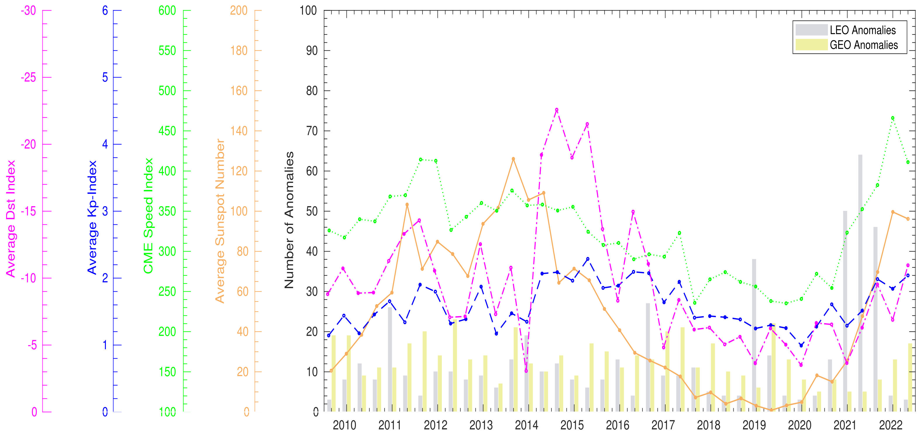
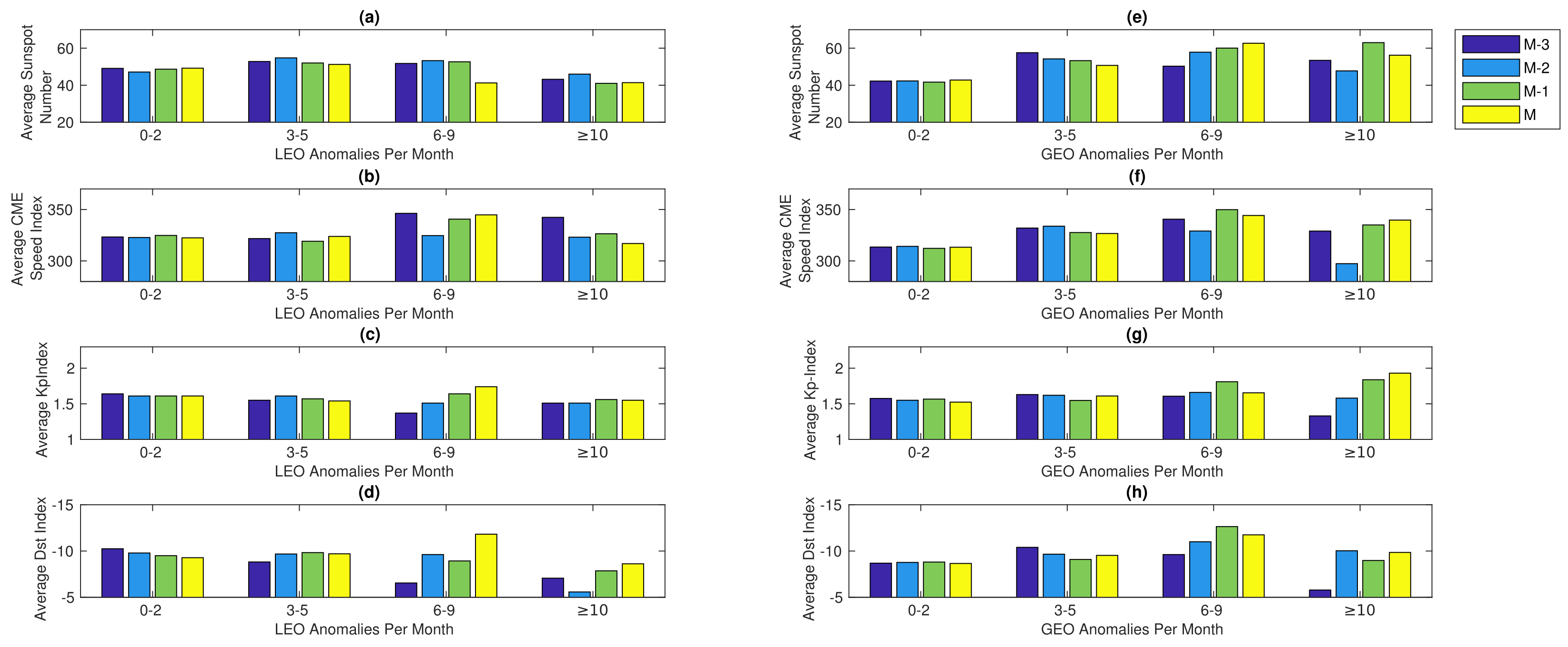
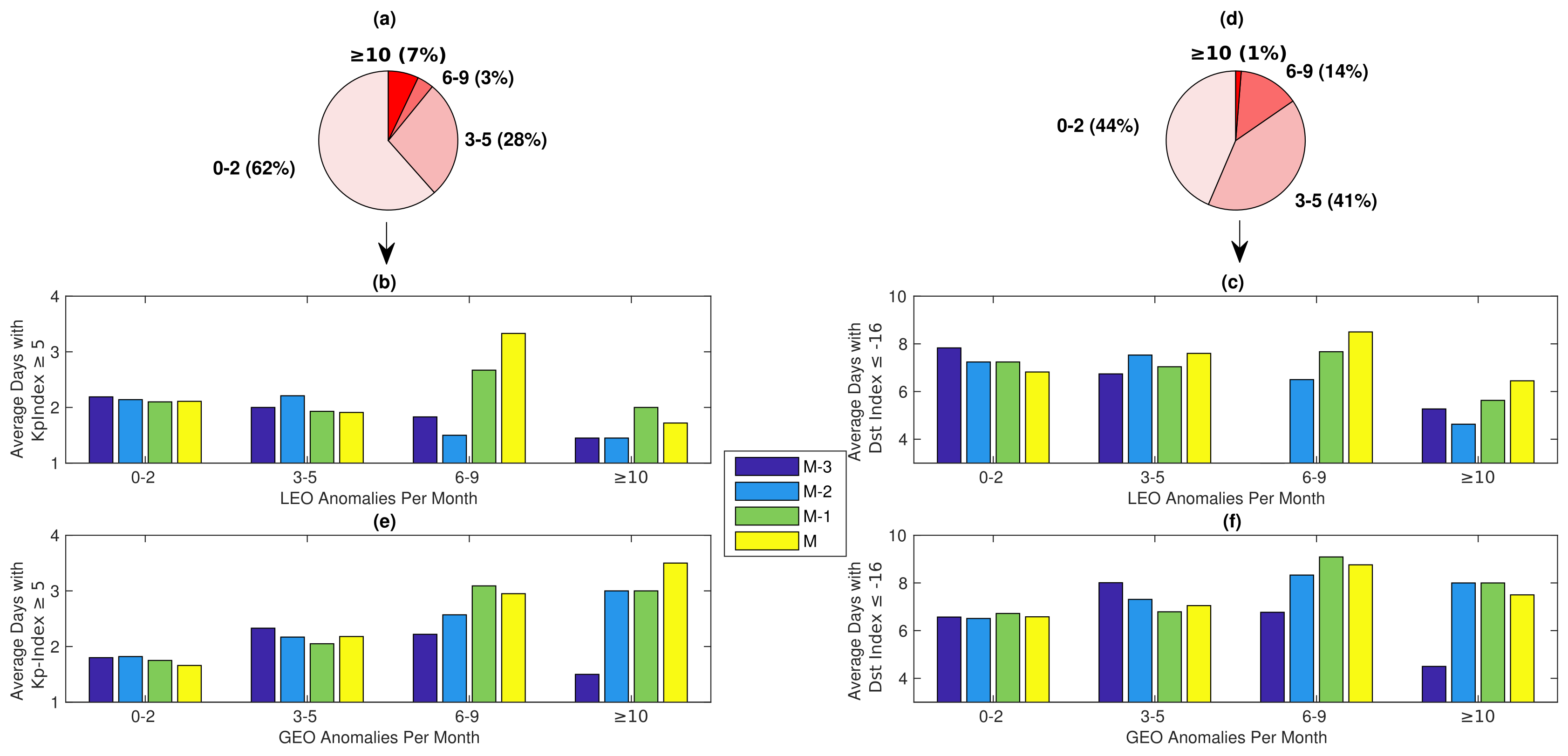
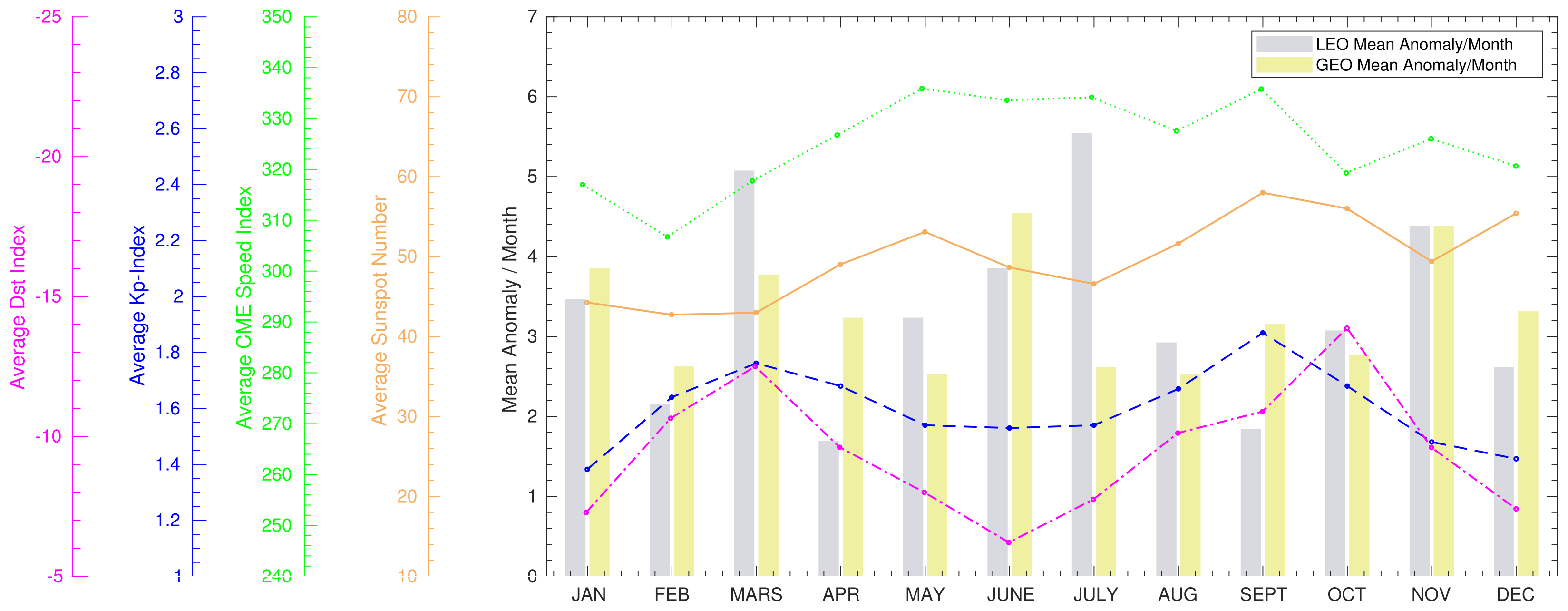
4.1. Monthly Analysis
Seasonal Variations
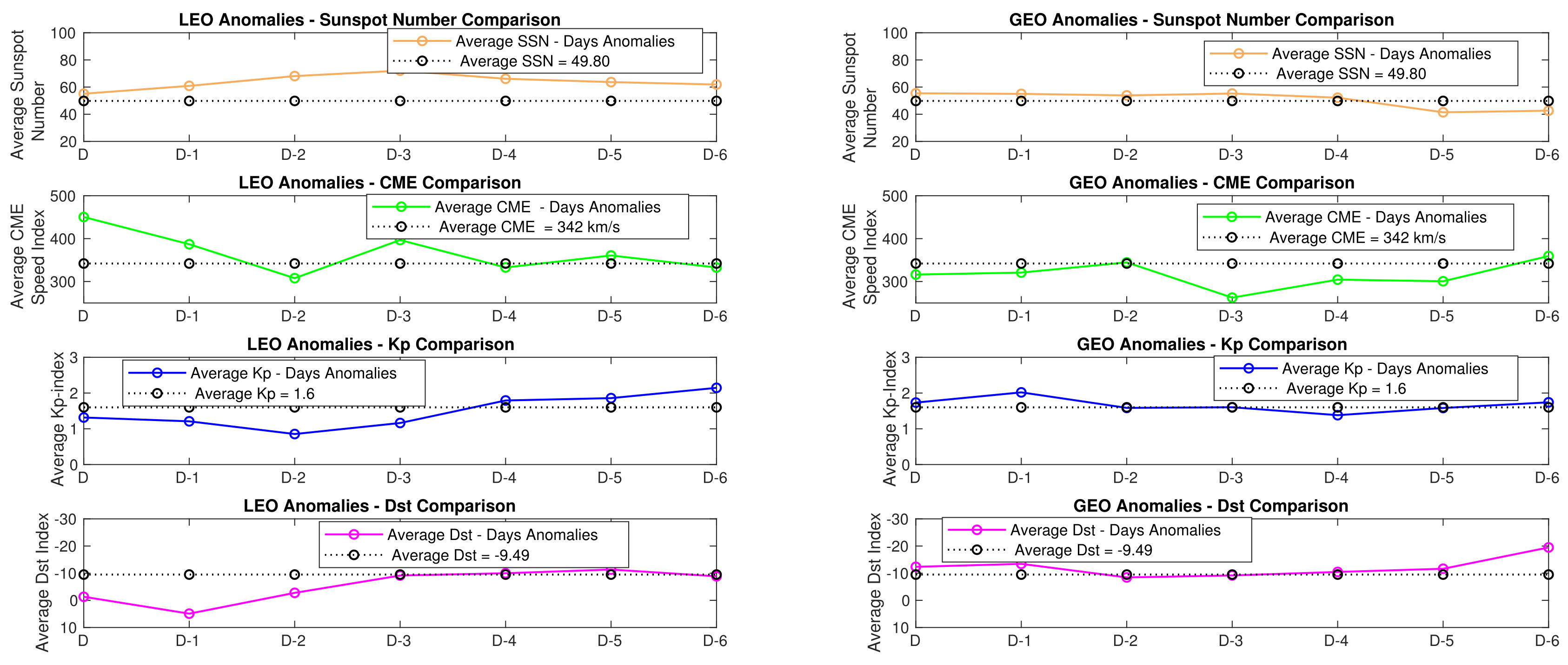
4.2. Daily Analysis
4.2.1. Solar and Magnetic Activity Assessment
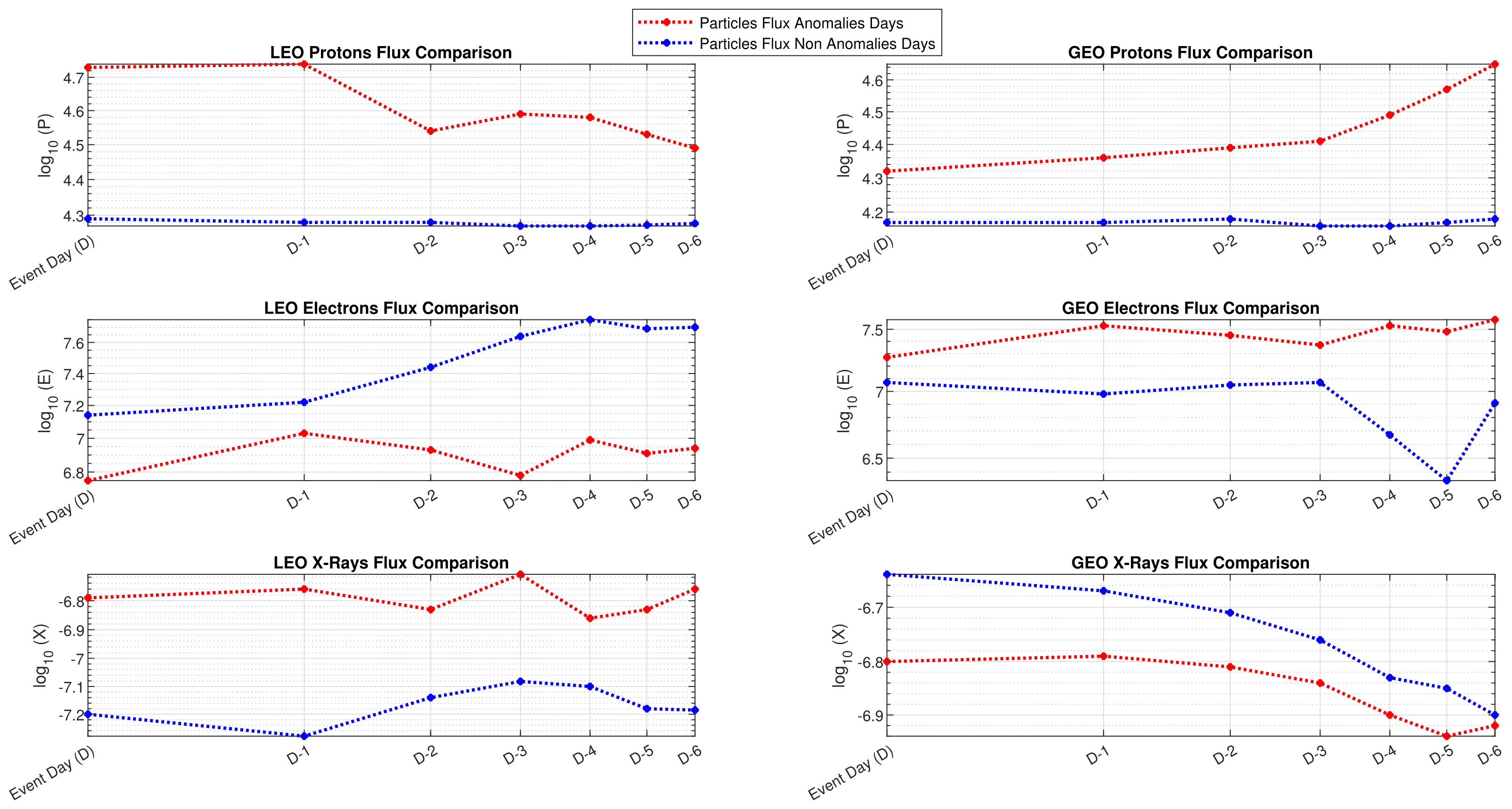
4.2.2. Particles Flux Density Assessment
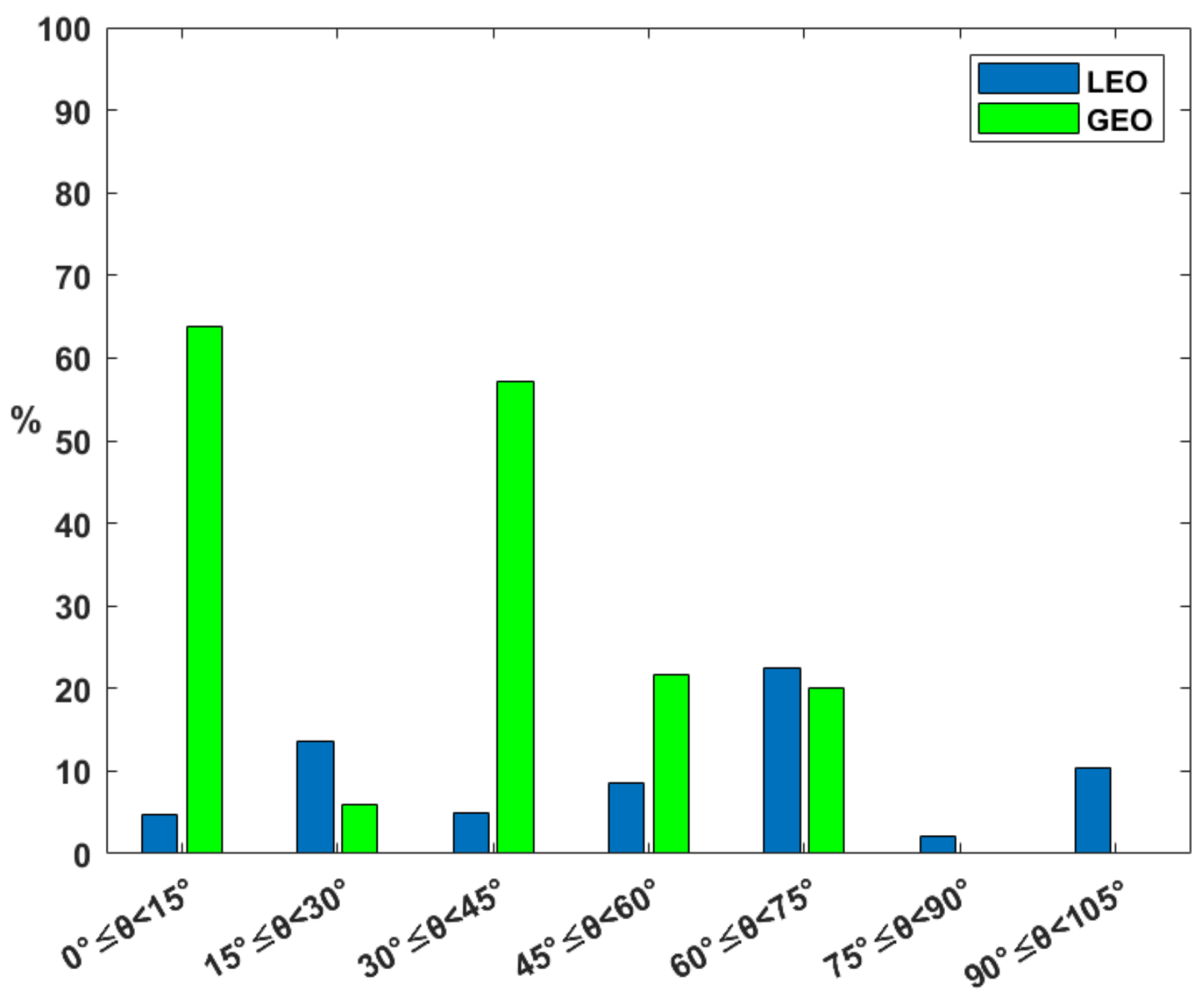
4.3. Orbit Inclination’s Impact on Anomaly Rate
5. Discussion and Conclusions
Author Contributions
Funding
Data Availability Statement
Conflicts of Interest
Abbreviations
| A | Number of Anomalies |
| Number of Anomalies per Day | |
| Number of Anomalies per Month | |
| ADCS | Attitude Determination Control System |
| BA | Brightness Asymmetry |
| CMEs | Coronal Mass Ejections |
| COMMS | Communication System |
| CPA | Central Position Angle |
| Dst | Disturbance Storm Time |
| EPS | Electrical Power System |
| ESA | European Space Agency |
| ESD | Electrostatic Discharge |
| FMPL-2 | Flexible Microwave Payload—Version 2 |
| FOV | Field of View |
| GCR | Galactic Cosmic Rays |
| GEO | Geosynchronous Orbit |
| LASCO | Large Angle and Spectrometric Coronagraph |
| LEO | Low Earth Orbit |
| NASA | National Aeronautics and Space Administration |
| NOAA | National Oceanic and Atmospheric Administration |
| OA | Outline Asymmetry |
| OBC | On-Board Computer |
| RadHard | Radiation Hardened |
| SAA | South Atlantic Anomaly |
| SEB | Single Event Burnout |
| SEL | Single Event Latch-up |
| SEU | Single Event Upset |
| SOHO | Solar and Heliospheric Observatory Satellite |
| SPEs | Solar Particle Events |
| SSN | Sunspot Number |
| TD | Total Dose |
| TT&C | Telemetry, Tracking, and Command |
| UV | Ultraviolet |
References
- Telastra Inc. Public Record Satellite Anomaly Database (PRSADB). 2021. Communications Satellite Databases. Available online: https://scholar.google.com/scholar_lookup?title=Communications%20satellite%20databases&publication_year=2021&author=N.H.%20Telastra%20Inc.Public%20Record%20Satellite%20Anomaly%20Database%20(PRSADB) (accessed on 2 February 2022).
- Jacklin, S.A. Small-Satellite Mission Failure Rates. 2019. Available online: https://ntrs.nasa.gov/api/citations/20190002705/downloads/20190002705.pdf (accessed on 11 July 2024).
- Quan, L.; Wang, D.; Zhang, Q.; Zhang, S.; Li, L.; Wang, S.; Jing, T.; Meng, Y.; Liu, Y.; Tian, C. Radiation environment and effect detection based on global navigation constellation. Open Astron. 2023, 32, 20220204. [Google Scholar] [CrossRef]
- Venkatesan, A.; Lowenthal, J.; Prem, P.; Vidaurri, M. The impact of satellite constellations on space as an ancestral global commons. Nat. Astron. 2020, 4, 1043–1048. [Google Scholar] [CrossRef]
- Novak, J.; Hastings, D. Analysis of proliferated low Earth orbit constellation resilience against solar weather radiation effects. Acta Astronaut. 2023, 202, 292–302. [Google Scholar] [CrossRef]
- Ecoffet, R. Overview of in-orbit radiation induced spacecraft anomalies. IEEE Trans. Nucl. Sci. 2013, 60, 1791–1815. [Google Scholar] [CrossRef]
- Mullen, E. Space Radiation Environments for Parts Selection/Test Considerations in Typical Satellite Orbits; Tech. Rep.; Assurance Technology Corporation: Carlisle, MA, USA, 2003; Volume 1. [Google Scholar]
- Tribble, A.C. The Space Environment: Implications for Spacecraft Design-revised and Expanded Edition; Princeton University Press: Princeton, NJ, USA, 2020. [Google Scholar]
- Purvis, C.K.; Garrett, H.B.; Whittlesey, A.C.; Stevens, N.J. Design Guidelines for Assessing and Controlling Spacecraft Charging Effects; National Aeronautics and Space Administration: Washington, DC, USA, 1984. [Google Scholar]
- Jia, X.; Liu, J.; Zhang, X. The Analysis of Ionospheric TEC Anomalies Prior to the Jiuzhaigou Ms7.0 Earthquake Based on BeiDou GEO Satellite Data. Remote Sens. 2024, 16, 660. [Google Scholar] [CrossRef]
- Iucci, N.; Levitin, A.E.; Belov, A.V.; Eroshenko, E.A.; Ptitsyna, N.G.; Villoresi, G.; Chizhenkov, G.V.; Dorman, L.I.; Gromova, L.I.; Parisi, M.; et al. Space weather conditions and spacecraft anomalies in different orbits. Space Weather 2005, 3, 16. [Google Scholar] [CrossRef]
- Choi, H.-S.; Lee, J.; Cho, K.-S.; Kwak, Y.-S.; Cho, I.-H.; Park, Y.-D.; Kim, Y.-H.; Baker, D.N.; Reeves, G.D.; Lee, D.-K. Analysis of GEO spacecraft anomalies: Space weather relationships. Space Weather 2011, 9, S06001. [Google Scholar] [CrossRef]
- Pilipenko, V.; Yagova, N.; Romanova, N.; Allen, J. Statistical relationships between satellite anomalies at geostationary orbit and high-energy particles. Adv. Space Res. 2006, 37, 1192–1205. [Google Scholar] [CrossRef]
- Paladini, S. The New Frontiers of Space; Springer: Berlin/Heidelberg, Germany, 2019. [Google Scholar]
- Foreman Campins, L. NewSpace and the European Space Economy. Master’s Thesis, Universitat Politècnica de Catalunya, Barcelona, Spain, 2023. [Google Scholar]
- Cloitre, A.; Dos Santos Paulino, V.; Theodoraki, C. The quadruple/quintuple helix model in entrepreneurial ecosystems: An institutional perspective on the space case study. R&D Manag. 2023, 53, 675–694. [Google Scholar]
- Mertens, C.J.; Kress, B.T.; Wiltberger, M.; Tobiska, W.K.; Grajewski, B.; Xu, X. Atmospheric Ionizing Radiation from Galactic and Solar Cosmic Rays; InTech Open Access Publisher: Rijeka, Croatia, 2012. [Google Scholar]
- Serrano Gonçalves, P.C. The Ionising Radiation Environment in the Solar System. 2021. Available online: https://pages.lip.pt/space/wp-content/uploads/sites/9/2023/02/The-Ionising-Radiation-Environment-in-the-Solar-System-Lesson.pdf (accessed on 2 February 2022).
- Miroshnichenko, L. Energetic Particles in the Geosphere. In Solar-Terrestrial Relations: From Solar Activity to Heliobiology; Springer: Berlin/Heidelberg, Germany, 2023; pp. 123–148. [Google Scholar]
- Miroshnichenko, L.I. Solar cosmic rays: 75 years of research. Phys. Uspekhi 2018, 61, 323. [Google Scholar] [CrossRef]
- Xu, J.; Guo, M.; Lu, M.; He, H.; Yang, G.; Xu, J. Effect of Alpha-Particle Irradiation on InGaP/GaAs/Ge Triple-Junction Solar Cells. Materials 2018, 11, 944. [Google Scholar] [CrossRef] [PubMed]
- Waets, A.; Bilko, K.; Coronetti, A.; Emriskova, N.; Barbero, M.S.; Alia, R.G.; Durante, M.; Schuy, C.; Wagner, T.; Esposito, L.S.; et al. Very-High-Energy Heavy Ion Beam Dosimetry using Solid State Detectors for Electronics Testing. IEEE Trans. Nucl. Sci. 2024, 71, 1837–1845. [Google Scholar] [CrossRef]
- Lu, Y.; Shao, Q.; Yue, H.; Yang, F. A review of the space environment effects on spacecraft in different orbits. IEEE Access 2019, 7, 93473–93488. [Google Scholar] [CrossRef]
- Barth, J.L. Space and atmospheric environments: From low earth orbits to deep space. In Protection of Materials and Structures from Space Environment: ICPMSE-6; Springer: Berlin/Heidelberg, Germany, 2004; pp. 7–29. [Google Scholar]
- Ya’acob, N.; Zainudin, A.; Magdugal, R.; Naim, N.F. Mitigation of space radiation effects on satellites at Low Earth Orbit (LEO). In Proceedings of the 6th IEEE International Conference on Control System, Computing and Engineering ICCSCE2016, Penang, Malaysia, 25–27 June 2016; pp. 56–61. [Google Scholar]
- Baker, D.N.; Erickson, P.J.; Fennell, J.F.; Foster, J.C.; Jaynes, A.N.; Verronen, P.T. Space Weather Effects in the Earth’s Radiation Belts. Space Sci. Rev. 2018, 214, 17. [Google Scholar] [CrossRef]
- McMurchie, E.J. Quantifying Radiation Effects of Energetic Electron Precipitation from the Van Allen Radiation Belts into the Earth’s Atmosphere. Master’s Thesis, University of Colorado at Boulder, Boulder, CO, USA, 2022. [Google Scholar]
- Bolin, J.A. Comparative Analysis of Selected Radiation Effects in Medium Earth Orbits. Ph.D. Thesis, Naval Postgraduate School, Monterey, CA, USA, 1997. [Google Scholar]
- Baker, D.N. Satellite anomalies due to space storms: The effects of space weather on spacecraft systems and subsystems; Space Storms and Space Weather Hazards; Springer: Berlin/Heidelberg, Germany, 2001; pp. 285–311. [Google Scholar]
- Garrett, H.B.; Close, S. Impact-induced ESD and EMI/EMP effects on spacecraft—A review. IEEE Trans. Plasma Sci. 2013, 41, 3545–3557. [Google Scholar] [CrossRef]
- Jun, I.; Garrett, H.; Kim, W.; Zheng, Y.; Fung, S.F.; Corti, C.; Ganushkina, N.; Guo, J. A review on radiation environment pathways to impacts: Radiation effects, relevant empirical environment models, and future needs. Adv. Space Res. 2024. ISSN 0273-1177. [Google Scholar] [CrossRef]
- Nwankwo, V.U.J.; Jibiri, N.N.; Kio, M.T. The Impact of Space Radiation Environment on Satellites Operation in Near-Earth Space. In Satellites Missions and Technologies for Geosciences; IntechOpen: London, UK, 2020; Volume 1, pp. 73–90. [Google Scholar]
- Johnson, R.E.; Carlson, R.W.; Cooper, J.F.; Paranicas, C.; Moore, M.H.; Wong, M.C. Radiation effects on the surfaces of the Galilean satellites. In Jupiter: The Planet, Satellites and Magnetosphere; Cambridge University Press: Cambridge, UK, 2004; Volume 1, pp. 485–512. [Google Scholar]
- Qiu, F.; Gong, J.; Tong, G.; Han, S.; Zhuang, X.; Zhu, X. Near-infrared Light-Induced Polymerizations: Mechanisms and Applications. ChemPlusChem 2024, 89, e202300782. [Google Scholar] [CrossRef]
- Likar, J.J.; Bogorad, A.; August, K.A.; Lombardi, R.E.; Kannenberg, K.; Herschitz, R. Spacecraft Charging, Plume Interactions, and Space Radiation Design Considerations for All-Electric GEO Satellite Missions. IEEE Trans. Plasma Sci. 2015, 43, 3099–3108. [Google Scholar] [CrossRef]
- Schwadron, N.A.; Cooper, J.F.; Desai, M.; Downs, C.; Gorby, M.; Jordan, A.P.; Joyce, C.J.; Kozarev, K.; Linker, J.A.; Mikíc, Z.; et al. Particle Radiation Sources, Propagation and Interactions in Deep Space, at Earth, the Moon, Mars, and Beyond: Examples of Radiation Interactions and Effects. Space Sci. Rev. 2017, 212, 1069–1106. [Google Scholar] [CrossRef]
- Fortescue, P.; Swinerd, G.; Stark, J. Spacecraft Systems Engineering; John Wiley & Sons: Hoboken, NJ, USA, 2011. [Google Scholar]
- SpaceTrack. SpaceTrack database: Number of Spacecraft’s Launches 2010–2023. Available online: https://spacetrak.seradata.com/Queries (accessed on 1 April 2024).
- Agency European Space. EO PORTAL. Available online: https://www.eoportal.org/ (accessed on 30 November 2022).
- National Aeronautics and Space Administration. Small Satellites Mission Failures Rate [Online]. Available online: https://ntrs.nasa.gov/citations/20190002705 (accessed on 12 December 2022).
- Buitrago-Leiva, J.N.; El Khayati Ramouz, M.; Camps, A.; Ruiz-de-Azua, J.A. Towards a second life for Zombie Satellites: Anomaly occurrence and potential recycling assessment. Acta Astronaut. 2024, 217, 238–245. [Google Scholar] [CrossRef]
- Zheng, Y.; Ganushkina, N.Y.; Jiggens, P.; Jun, I.; Meier, M.; Minow, J.I.; O’Brien, T.P.; Pitchford, D.; Shprits, Y.; Tobiska, W.K.; et al. Space Radiation and Plasma Effects on Satellites and Aviation: Quantities and Metrics for Tracking Performance of Space Weather Environment Models. Space Weather 2019, 17, 1384–1403. [Google Scholar] [CrossRef] [PubMed]
- Stassinopoulos, E.; Brucker, G.; Adolphsen, J.; Barth, J. Radiation-induced anomalies in satellites. J. Spacecr. Rocket. 1996, 33, 877–882. [Google Scholar] [CrossRef]
- NASA. Solar Activity. Available online: https://spaceplace.nasa.gov/solar-activity/en/ (accessed on 23 April 2024).
- Royal Observatory of Belgium. 2024. Available online: http://www.sidc.be/silso/home (accessed on 12 April 2024).
- NOAA National Centers for Environmental Information. Kp and Ap indices. 2024. Available online: https://www.ngdc.noaa.gov/geomag/indices/kp_ap.html (accessed on 12 April 2024).
- Bryant, K.; Young, R.P.; LeFevre, H.J.; Kuranz, C.C.; Olson, J.R.; McCollam, K.J.; Forest, C.B. Creating and studying a scaled interplanetary coronal mass ejection. Phys. Plasmas 2024, 31, 042901. [Google Scholar] [CrossRef]
- Jain, S.; Podladchikova, T.; Chikunova, G.; Dissauer, K.; Veronig, A.M. Coronal dimmings as indicators of the direction of early coronal mass ejection propagation. Astron. Astrophys. 2024, 683, A15. [Google Scholar]
- Singh, R.; Powar, V. The Future of Generation, Transmission, and Distribution of Electricity. In The Advancing World of Applied Electromagnetics: In Honor and Appreciation of Magdy Fahmy Iskander; Springer: Berlin/Heidelberg, Germany, 2024; pp. 349–383. [Google Scholar]
- NASA.SOHO LASCO CME CATALOG—Version 2. Available online: https://cdaw.gsfc.nasa.gov/CME_list/UNIVERSAL_ver2/1996_01/univ1996_01.html (accessed on 2 February 2024).
- Solanki, S.K.; Teriaca, L.; Barthol, P.; Curdt, W.; Inhester, B. European Solar Physics: Moving from SOHO to Solar Orbiter and Beyond. Mem. Soc. Astron. Ital. 2013, 84, 286. [Google Scholar]
- Kilcik, A.; Yurchyshyn, V.B.; Abramenko, V.; Goode, P.R.; Gopalswamy, N.; Ozguc, A.; Rozelot, J.P. Maximum Coronal Mass Ejection Speed as an Indicator of Solar and Geomagnetic Activities. Astrophys. J. 2011, 727, 44. [Google Scholar] [CrossRef]
- Welling, D.T. The long-term effects of space weather on satellite operations. Ann. Geophys. 2010, 28, 1361–1367. [Google Scholar] [CrossRef]
- Tacza, J.; Li, G.; Raulin, J.-P. Effects of Forbush Decreases on the global electric circuit. Space Weather 2024, 22, e2023SW003852. [Google Scholar] [CrossRef]
- Banerjee, A.; Bej, A.; Chatterjee, T.N. On the existence of a long range correlation in the geomagnetic disturbance storm time (Dst) index. Astrophys. Space Sci. 2012, 337, 23–32. [Google Scholar] [CrossRef]
- Dachev, T.P. South-Atlantic Anomaly magnetic storms effects as observed outside the International Space Station in 2008–2016. J. Atmos. Sol. Terr. Phys. 2018, 179, 251–260. [Google Scholar] [CrossRef]
- Kyoto University. Dst Provisional Values. Available online: https://wdc.kugi.kyoto-u.ac.jp/dst_provisional/index.html (accessed on 1 February 2024).
- Filippov, B.P. Mass ejections from the solar atmosphere. Phys. Uspekhi 2019, 62, 847. [Google Scholar] [CrossRef]
- Boenig, H. Plasma Science and Technology; Cornell University Press: Ithaca, NY, USA, 2019. [Google Scholar]
- Space Weather Prediction Center, National Oceanic and Atmospheric Administration. GOES Electron Flux. 2024. Available online: https://www.swpc.noaa.gov/products/goes-electron-flux (accessed on 10 April 2024).
- Space Weather Prediction Center, National Oceanic and Atmospheric Administration. GOES Proton Flux. 2024. Available online: https://www.swpc.noaa.gov/products/goes-proton-flux (accessed on 10 April 2024).
- Höeffgen, S.K.; Metzger, S.; Steffens, M. Investigating the effects of cosmic rays on space electronics. Front. Phys. 2020, 8, 318. [Google Scholar] [CrossRef]
- Ziemacki, T.; Drzazga, R. The impact of radiation on electronics in space: A review. Acta Astronaut. 2019, 157, 172–179. [Google Scholar] [CrossRef]
- The Bureau of Meteorology. Australian Space Weather Forecasting Centre. Meaning of X-Ray Fluxes From the Sun. 2024. Available online: https://www.sws.bom.gov.au/Educational/2/1/3 (accessed on 10 April 2024).
- Miteva, R.; Samwel, S.W.; Tkatchova, S. Space weather effects on satellites. Astronomy 2023, 2, 165–179. [Google Scholar] [CrossRef]
- Nirmal Kumar, R.; Ranjith Dev Inbaseelan, C.; Karthikeyan, E.; Nithyasree, M.; Johnson Jeyakumar, H. Analysis of solar energetic particle (SEP) event on the geomagnetic environment during 24th solar cycle. Astrophys. Space Sci. 2024, 369, 56. [Google Scholar]
- Rodriguez, L.; Shukhobodskaia, D.; Niemela, A.; Maharana, A.; Samara, E.; Verbeke, C.; Magdalenic, J.; Vansintjan, R.; Mierla, M.; Scolini, C.; et al. Validation of EUHFORIA cone and spheromak Coronal Mass Ejection Models. arXiv 2024, arXiv:2405.04637. [Google Scholar] [CrossRef]
- Camps, A.; Munoz-Martin, J.F.; Ruiz-de-Azua, J.A.; Fernandez, L.; Perez-Portero, A.; Llaveria, D.; Herbert, C.; Pablos, M.; Golkar, A.; Gutiérrez, A.; et al. FSSCat: The Federated Satellite Systems 3 Cat Mission: Demonstrating the capabilities of CubeSats to monitor essential climate variables of the water cycle [Instruments and Missions]. IEEE Geosci. Remote Sens. Mag. 2022, 10, 260–269. [Google Scholar] [CrossRef]
- NASA. NASA Lesson: Solar Flares and Their Effect on Earth’s Magnetosphere. 2024. Available online: https://llis.nasa.gov/lesson/824 (accessed on 12 May 2024).
- Nasuddin, K.A.; Abdullah, M.; Abdul Hamid, N.S. Characterization of the South Atlantic Anomaly. Nonlinear Process. Geophys. 2019, 26, 25–35. [Google Scholar] [CrossRef]
- Velazco, R.; Fouillat, P.; Reis, R. Radiation Effects on Embedded Systems; Springer: Dordrecht, The Netherlands, 2007. [Google Scholar]
- Samwel, S.W.; El-Aziz, E.A.; Garrett, H.B.; Hady, A.A.; Ibrahim, M.; Amin, M.Y. Space radiation impact on smallsats during maximum and minimum solar activity. Adv. Space Res. 2019, 64, 239–251. [Google Scholar] [CrossRef]

| LEO (9 Days) | GEO (16 Days) | |
|---|---|---|
| 15 July 2014 | 15 March 2010 | 15 October 2015 |
| 15 July 2017 | 30 June 2010 | 1 March 2016 |
| 6 May 2021 | 15 February 2011 | 12 June 2017 |
| 23 August 2021 | 15 March 2012 | 15 November 2017 |
| 21 November 2021 | 30 June 2012 | 15 May 2018 |
| 9 January 2022 | 15 November 2012 | 15 June 2018 |
| 15 August 2022 | 15 January 2013 | 5 November 2019 |
| 15 September-2022 | 15 January 2014 | - |
| 15 December 2022 | 30 June 2014 | - |
| LEO (6 Days) | GEO (6 Days) |
|---|---|
| 15 July 2014 | 15 October 2015 |
| 15 July 2017 | 1 March 2016 |
| 6 May 2021 | 12 June 2017 |
| 23 August 2021 | 15 November 2017 |
| 21 November 2021 | 15 May 2018 |
| 9 January 2022 | 15 June 2018 |
Disclaimer/Publisher’s Note: The statements, opinions and data contained in all publications are solely those of the individual author(s) and contributor(s) and not of MDPI and/or the editor(s). MDPI and/or the editor(s) disclaim responsibility for any injury to people or property resulting from any ideas, methods, instructions or products referred to in the content. |
© 2024 by the authors. Licensee MDPI, Basel, Switzerland. This article is an open access article distributed under the terms and conditions of the Creative Commons Attribution (CC BY) license (https://creativecommons.org/licenses/by/4.0/).
Share and Cite
Buitrago-Leiva, J.N.; El Khayati Ramouz, M.; Camps, A.; Ruiz-de-Azua, J.A. Statistical Analysis of LEO and GEO Satellite Anomalies and Space Radiation. Aerospace 2024, 11, 924. https://doi.org/10.3390/aerospace11110924
Buitrago-Leiva JN, El Khayati Ramouz M, Camps A, Ruiz-de-Azua JA. Statistical Analysis of LEO and GEO Satellite Anomalies and Space Radiation. Aerospace. 2024; 11(11):924. https://doi.org/10.3390/aerospace11110924
Chicago/Turabian StyleBuitrago-Leiva, Jeimmy Nataly, Mohamed El Khayati Ramouz, Adriano Camps, and Joan A. Ruiz-de-Azua. 2024. "Statistical Analysis of LEO and GEO Satellite Anomalies and Space Radiation" Aerospace 11, no. 11: 924. https://doi.org/10.3390/aerospace11110924
APA StyleBuitrago-Leiva, J. N., El Khayati Ramouz, M., Camps, A., & Ruiz-de-Azua, J. A. (2024). Statistical Analysis of LEO and GEO Satellite Anomalies and Space Radiation. Aerospace, 11(11), 924. https://doi.org/10.3390/aerospace11110924