Valley Path Planning on 3D Terrains Using NSGA-II Algorithm

Abstract

Valley path planning on 3D terrains holds significant importance in navigating and understanding complex landscapes. This specialized form of path planning focuses on finding optimal routes that adhere to the natural contours of valleys within three-dimensional terrains. The significance of valley path planning lies in its ability to address specific challenges presented by valleys, such as varying depths, steep slopes, and potential obstacles. By following the natural flow of valleys, path planning can enhance the efficiency of navigation and minimize the risk of encountering difficult terrain or hazards. In recent years, an increasing number of researchers have focused on the study of valley path planning on 3D terrains. This study presents a valley path planning method utilizing the NSGA-II (Non-dominated Sorting Genetic Algorithm II) approach. To ensure that the paths generated by the algorithm closely follow the valley lines, the algorithm establishes an optimization function that includes three optimization criteria: mean altitude, flight route length, and mean offset. To test the performance of this algorithm, we conducted experiments based on workspaces based on three datasets full of 3D terrains and compared it with three baseline algorithms. The evaluation indicates that the suggested algorithm successfully designs routes that closely follow the valley contours.

1. Introduction

Valley path planning on 3D terrain is an important research area in the field of robotics and autonomous systems, focusing on developing algorithms and methods for planning optimal paths in complex three-dimensional landscapes [1]. The emergence of this research area is driven by the increasing use of autonomous vehicles and robots in exploration, agriculture, search and rescue, and other applications that require navigation in complex natural environments. Valleys and similar terrains present unique challenges for path planning, as they often feature irregular and steep topography, limited visibility, and unpredictable environmental conditions. Traditional path planning methods, such as the A* algorithm, may not be suitable for these environments, as valley spaces are typically complex and non-convex. Research in the field of valley path planning aims to address these challenges by developing specialized algorithms that take into account specific features of valley terrain, such as narrow passages, potential dead ends, and varying slopes. By leveraging techniques from computational geometry, machine learning, and computer vision, researchers strive to create path planning algorithms that can efficiently traverse valley terrain while considering factors such as energy consumption, stability, and terrain traversability.

The research on valley path planning for aircraft holds significant importance, as aircraft often need to traverse various terrains, including complex landscapes such as valleys and canyons during flight. Planning optimal paths in these terrains is crucial for the safety and efficiency of aircraft.Furthermore, there is increasing attention on the autonomous control and navigation systems of aircraft, as these systems can enhance the safety, reliability, and efficiency of flights. The use of valley path planning methods on aircraft can help the autonomous control and navigation systems better adapt to complex terrains, thereby improving the safety and efficiency of flights. For unmanned aerial vehicles (UAVs), utilizing valley path planning can enhance accurate navigation through intricate landscapes while decreasing dependence on human operators. In military and civilian applications, UAVs are utilized for tasks such as reconnaissance, surveillance, and delivery, making it crucial to ensure that UAVs can accurately and safely traverse valleys and other complex terrains in these missions. In summary, the research background of applying valley path planning algorithms on aircraft includes the demand for autonomous navigation and control systems for aircraft, the requirements for flight safety, reliability, and efficiency, and the widespread deployment of drones in both military and civilian contexts.

When designing robots for outdoor settings, it is essential to take terrain characteristics into account during the route-planning process. C. Saranya et al. [2] introduced an enhanced version of the D* path planning algorithm. This method incorporates not only the distance to be covered but also an assessment of the terrain slope in the cost function calculations to determine the optimal path. Yoshitaka et al. [3] developed a technique for eliminating moving objects and constructing maps to facilitate path planning in three-dimensional environments. Their approach features a map type called surface mesh maps, created from 3D LIDAR data through a graph-based SLAM process that includes moving object removal and polygon mesh reconstruction. The key innovation of this technique lies in its integration of SLAM with object removal and graph search methods for navigating expansive 3D terrains. Experimental results from traversing over 5 km in dynamic outdoor settings demonstrated the effectiveness of this method in both object removal and surface mesh mapping for three-dimensional path planning. Cheng et al. [4] created a UAV route optimization technique designed to achieve the necessary image overlap and enhance flight paths for reconstructing digital terrain models (DTMs). Their findings indicated that this path-planning approach could cut UAV flight time for capturing images of the Put-tun-pu-nas debris fan by 18.5%. Boris et al. [5] focused on optimizing path planning for UAVs operating in a stable risk-free environment within three-dimensional space. Meanwhile, Zhan et al. [6] presented an optimized A* algorithm designed for real-time UAV navigation in extensive battlefield settings, addressing the need for high survival rates and reduced fuel usage. The authors evaluated their algorithm across an area of around 2,500,000 square meters, which included radar systems, restricted zones, and harsh weather conditions, to assess its practicality, reliability, and effectiveness. Sedat et al. [7] applied a genetic algorithm to enhance the solution for the CPP problem by focusing on energy efficiency while considering natural terrain factors such as obstacles and elevation changes. Field experiments validated their energy consumption model for the robot, and simulation findings demonstrated that their method successfully lowers the energy usage of a mobile robot engaged in CPP tasks. D.L. Page et al. [8] introduced a strategic path planning technique designed for unmanned vehicles to either maximize visibility by traveling along ridges or enhance stealth by moving through valleys in a 3D terrain. The approach aims to create routes that optimize either surveillance or covert operations based on the vehicle’s position within the terrain. Pablo et al. [9] developed an innovative heuristic path planning method called 3Dana. This algorithm aims to create long-term routes by taking into account the terrain’s relief. To showcase the effectiveness of 3Dana, the authors conducted comparisons with several other algorithms, including A*, Field D*, and Theta*, using traversability cost maps. The results indicate that 3Dana yields favorable outcomes, albeit with a longer search duration. Francis et al. [10] introduced a system capable of planning and navigating a route in intricate environments based on input from noisy sensors. Rekha et al. [11] introduced an innovative motion planning algorithm tailored designed for a six-wheeled robot featuring 10 degrees of freedom, enhancing the traditional potential field approach by incorporating a gradient function. The revised potential field comprises attractive, repulsive, tangential, and gradient forces. Both simulation and experimental findings demonstrate the effectiveness of this method in creating paths across challenging terrains.

However, the aforementioned algorithm exhibits poor global search capability, especially when dealing with large-scale 3D elevation maps. It also shows limited robustness, as specific algorithms can only address particular workspaces, and it cannot handle path search problems with multiple constraints and optimization objectives.

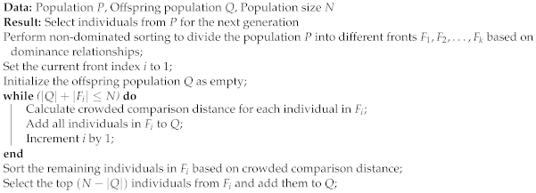
NSGA-II is designed for optimizing multiple objectives and developed to handle problems involving several competing objectives. Building upon the principles of genetic algorithms, NSGA-II aims to find a set of solutions that are non-dominated by any other solutions, meaning there are no better solutions that simultaneously improve all objectives. It achieves this by employing non-dominated sorting and crowding distance operator to maintain diversity within the population, thus providing an efficient and balanced set of solutions for multi-objective optimization problems. NSGA-II has proven to be a powerful tool for tackling complex real-world problems in various domains such as engineering design, resource allocation, and decision support systems. The NSGA-II algorithm has several advantages. Firstly, it is capable of efficiently handling multi-objective optimization problems by simultaneously optimizing multiple conflicting objectives. Secondly, NSGA-II employs a fast and elitist non-dominated sorting approach, which allows it to maintain a diverse set of solutions along the Pareto front. Additionally, NSGA-II utilizes a crowding distance to promote solution diversity, enabling it to effectively explore and maintain a well-distributed set of non-dominated solutions. These characteristics make NSGA-II a robust and widely algorithm utilized for addressing multiple objective optimization issues, offering a good balance between convergence and diversity in the obtained solutions.

Nikolas et al. [12] presented a comprehensive strategy to address the Multi-Objective Path Planning (MOPP) challenge for UAVs navigating in a vast 3D urban landscape. They introduced an energy and noise model for UAVs to follow a continuous 3D trajectory, utilizing the NSGA-II algorithm for optimization. This approach was tested in a practical 3D urban planning scenario in New York City, leveraging real-world data from OpenStreetMap. The study in [13] introduced an improved NSGA-II algorithm designed to address the multi-objective path planning challenge for UAVs in authentic 3D environments, aiming to identify a safe and energy-efficient route. Experimental results demonstrate that the enhanced NSGA-II (ENSGAII) exhibits superior convergence rates and solution diversity across various new real-world datasets. Ren et al. [14] introduced a multi-objective path planning (MOPP) method utilizing the NSGA-II algorithm to determine an ideal collision-free trajectory for UAVs, factoring in distance. Their experiments show that this method efficiently identifies optimal paths in urban settings using octrees. The work presented in [15] introduces an enhanced version of the NSGA-II algorithm (INSGA-II) aimed at tackling multi-objective path planning challenges by concurrently optimizing path length, safety, and smoothness. Simulation findings reveal that INSGA-II effectively addresses these multi-objective path planning issues with notable efficiency. Carlos et al. [16] introduced a novel system designed to assist with multi-objective path planning for gliders in actual missions. This system integrates a path simulator with the NSGA-II genetic algorithm, generating a range of Pareto-optimal solutions focused on two main objectives: distance to the goal and trajectory safety. Various experiments were conducted to thoroughly evaluate the proposed system. The findings indicate that it can efficiently identify multiple Pareto-optimal solutions in scenarios with static obstacles. Furthermore, this approach is practical for real missions, as it does not require high-end computing resources. In the study [17], a NSGA-II method for optimizing spray trajectories is introduced. The effectiveness of this method is validated on actual automotive surfaces, with results demonstrating its capability in addressing trajectory planning challenges on intricate surfaces. In [18], a many-objective optimization model for cooperative UAV trajectory planning is presented. This model aims to optimize various factors including trajectory distance, time, threat levels, and coordination costs. To address traditional trajectory planning issues, the NSGA-III algorithm is employed. Additionally, the study introduces a segmented crossover technique and a dynamic crossover probability in the crossover operator to enhance the model’s efficiency and speed up the algorithm’s convergence. Experimental outcomes validate the effectiveness of this multi-UAV cooperative trajectory planning method in meeting diverse practical requirements. P.B. Muilk [19] introduced an innovative trajectory planning method for the PUMA 560 robot manipulator, utilizing an evolutionary algorithm. This approach, based on the elitist non-dominated sorting genetic algorithm (NSGA-II), stands out due to its ability to optimize multiple criteria concurrently.

The current research on valley line path planning faces the following issues: first, although there has been considerable study on 3D terrains, research specifically focused on valley line path planning, especially in multi-objective optimization under various constraints, remains limited. Second, existing valley point path planning algorithms exhibit low efficiency in processing valley points, resulting in overall low planning efficiency and longer planning times. Furthermore, the existing algorithms for 3D terrain path planning lack sufficient planning efficiency and often become trapped in local optima, producing suboptimal paths. To address these issues, this study introduces an algorithm for planning valley paths that is grounded in NSGA-II designed for 3D terrains. Firstly, the problem statement is defined. Secondly, the NSGA-II-based valley path planning algorithm is introduced. Within the NSGA-II-based valley path planning algorithm, the NSGA-II Algorithm is first described, followed by the valley path planning algorithm on 3D terrains designed using the NSGA-II algorithm. Subsequently, the algorithm validation is conducted in the experimental study. In the experimental study, workspaces using three DEM datasets are first introduced, followed by the demonstration of validation results based on the three datasets and four algorithms (the NSGA-II based valley path planning algorithm and three baseline algorithms).

This paper is organized as follows: In Section 2, we define the problem of valley path planning using mathematical symbols. In Section 3, we introduce the NSGA-II-based algorithm, including an overview of NSGA-II algorithms and how to apply NSGA-II to valley path planning problems. In Section 4, we conduct experiments on three datasets using four different algorithms (NSGA-II-based valley path planning algorithm and three other baseline algorithms). Conclusions are drawn in Section 5.

2. Problem Definition

Define ${\rm Y}$ as a cubic workspace filled with 3D terrains. Based on this workspace, we carry out the valley line path planning task. This task is defined as a multi-constraint multi-objective problem. The constraints include aircraft kinematic constraints (minimum turning radius constraint $R_{min}$), terrain constraints $O_t$ (obstacle and terrain constraints), and valley point constraints $V_c$ (the planned path should follow the valley line as closely as possible); the optimization objectives include flight route length L, deviation from valley points $D_e$, and average altitude of route points $H_a$.

Our goal is to plan a valley line path ${\Gamma }_v$ that meets the three optimization objectives of flight route length L, deviation from valley points $V_c$, and average altitude of route points $H_a$ while satisfying aircraft kinematic constraints, terrain constraints, and valley point constraints.  

$$\begin{array}{cc}\hfill \mathrm{minimize}& L,D_e,H_a\hfill \\ \hfill \mathrm{subject}\mathrm{to}& R\ge R_{\min }\hfill \\ \hfill & {\Gamma }_v\cap O_t=\varnothing \hfill \\ \hfill & {\Gamma }_v\approx V_c\hfill \end{array}$$

(1)

where calculation methods of L, $D_e$, and $H_a$, respectively will be introduced in Section 3.

The main content of this paper is defined as follows: In the context of task scenarios filled with 3D terrains, the NSGA-II algorithm is used to solve the multi-objective optimization problem of flight route planning. Specifically, this paper aims to plan a valley path that satisfies three optimization objectives: mean altitude, flight route length, and mean offset, while considering the minimum turning radius and terrain constraints.

3. NSGA-II-Based Valley Path Planning Algorithm

3.1. Valley Feature-Based Valley Detection Algorithm

3.1.1. Valley Feature

The notion of a valley point in a mathematical context refers to a point in a function’s domain where the function reaches a local minimum surrounded by higher values. Mathematically, a valley point can be described as a point p such that there exists a neighborhood around p where the function value at p is lower than the function values at all other points in the neighborhood.

To detect valley points in a function, one common method is to utilize the first and second derivatives of the function. Specifically, a point p can be considered a potential valley point if the following conditions are satisfied:

The first derivative at p is zero, indicating a potential extremum.

$$\begin{array}{c}{\displaystyle \frac{dp}{dx}}=0\end{array}$$

(2)

The second derivative at $p_v$ is positive, indicating a local minimum.

$$\begin{array}{c}{\displaystyle \frac{d^{2}p}{d{x}^2}}>0\end{array}$$

(3)

By analyzing the function’s behavior at locations in cases where the first derivative is zero, while the second derivative remains positive, potential valley points can be determined. Further analysis, such as checking the concavity of the function and confirming the presence of a local minimum, can help validate whether a point is indeed a valley point in the function’s domain.

3.1.2. Valley Detection

Our approach to valley point detection is as follows: inspired by the literature [20], we employ a sliding window of a certain size to traverse the entire elevation map, identifying all local minima points. Subsequently, we utilize the mathematical characteristics of valley points to further refine and pinpoint the valley points within the dataset.

3.2. B-Spline

B-Spline interpolation is a popular technique used in computer graphics and numerical analysis for curve and surface fitting. B-Splines are piecewise polynomial functions that have local control properties, making them flexible and efficient for representing complex curves and surfaces. In B-Spline interpolation, a smooth curve or surface is constructed by fitting a series of B-Spline basis functions to the given data points. These basis functions are combined to generate a continuous curve or surface that interpolates the data points while ensuring smoothness and continuity at the control points.

If there are $m+1$ control points $P_0$, $P_1$, …, $P_n$ in the space, then an nth degree B-spline curve can be represented as

$$\begin{array}{c}S\left(t\right)={\displaystyle \sum _{i=0}^m}{P}_i{b}_{i,n}\left(t\right),t\in [0,1]\end{array}$$

(4)

In Equation (5), ${\mathrm{b}}_{\mathrm{i},\mathrm{n}}\left(\mathrm{t}\right),\mathrm{t}\in [0,1]$ represents B-Spline basis functions of degrees of n. The m + 1 nth degree B-spline basis functions can be defined using the Cox-deBoor recursive formula.

$$\begin{array}{c}{b}_{j,0}\left(t\right):=\left\{\begin{array}{cc}1\hfill & t_j<t<t_{j+1}\hfill \\ 0\hfill & \dots \hfill \end{array}\right.\end{array}$$

(5)

$$\begin{array}{c}{b}_{j,n}\left(t\right):={\displaystyle \frac{t-t_j}{t_{j+n}-t_j}}{b}_{j,n-1}\left(t\right)+{\displaystyle \frac{t_{j+n+1}-t}{t_{j+n+1}-t_{j+1}}}{b}_{j+1,n-1}\left(t\right)\end{array}$$

(6)

References [21,22,23,24,25] provides us with the derivation of the coordinates of B-Spline curves based on the following formula:

$$\begin{array}{c}X\left(t\right)={\displaystyle \sum _{i=0}^n}{b}_{i,n}\left(t\right)·x_i\end{array}$$

(7)

$$\begin{array}{c}Y\left(t\right)={\displaystyle \sum _{i=0}^n}{b}_{i,n}\left(t\right)·y_i\end{array}$$

(8)

$$\begin{array}{c}Z\left(t\right)={\displaystyle \sum _{i=0}^n}{b}_{i,n}\left(t\right)·z_i\end{array}$$

(9)

One of the key advantages of B-Spline interpolation is its ability to provide local control over the shape of the interpolated curve or surface, allowing for easy manipulation of individual control points without affecting the rest of the curve or surface. This property makes B-Spline interpolation a powerful tool for a wide range of applications, including computer-aided design, image processing, and geometric modeling.

3.3. NSGA-II-Based Valley Path Planning Algorithm

NSGA-II is a popular algorithm for solving multi-objective optimization issues with conflicting goals. Based on genetic algorithms, NSGA-II focuses on finding a solution set that is not dominated by any other solutions with respect to all objectives simultaneously. To achieve this, NSGA-II applies non-dominated sorting along with crowding distance to ensure a varied solution population. This strategy helps NSGA-II effectively explore the trade-off between different objectives and produce a well-distributed set of Pareto-optimal solutions [26,27,28,29,30].

NSGA-II is a multi-objective optimization algorithm that leverages various key components to efficiently search for a diverse set of Pareto-optimal solutions. The algorithm utilizes the concepts of domination and non-domination, where one solution is said to dominate another if it is better in at least one objective and not worse in any other objective. Pareto-optimal solutions are those that cannot be improved in one objective without sacrificing performance in another.

To maintain diversity and convergence toward the Pareto front, NSGA-II incorporates several key operators and strategies. Firstly, it employs non-dominated sorting to classify solutions into different fronts based on their dominance relationships. This allows the algorithm to identify the most promising solutions that are not dominated by any others. Additionally, NSGA-II utilizes the crowding distance metric to encourage solutions to spread evenly across the Pareto front, promoting well-spread solutions. NSGA-II also implements an elite strategy to preserve the best solutions from one generation to the next, ensuring that promising solutions are not lost during the evolutionary process. The selection operation in NSGA-II is based on a combination of non-dominated sorting and crowding distance. Furthermore, NSGA-II incorporates genetic operators, including crossover and mutation, to generate offspring solutions from parent solutions. These operators are applied with a balance between exploration and exploitation to efficiently explore the search space and refine solutions toward the Pareto front.

3.3.1. Pareto Optimality

Pareto optimal solutions, named after the Italian economist Vilfredo Pareto, represent a set of solutions in multi-objective optimization where no solution can be improved in one objective without degrading performance in at least one other objective. In other words, a solution is considered Pareto optimal if there is no alternative solution that is better in all objectives simultaneously. The concept of Pareto optimality is central to multi-objective optimization, as it highlights the trade-offs and inherent conflicts between different objectives. By identifying Pareto-optimal solutions, decision-makers can explore a spectrum of solutions that represent different compromises between competing objectives.

Algorithm 1: Pareto optimality identification

The provided pseudo-code (see Algorithm 1) illustrates the process of identifying Pareto-optimal solutions within a population P and storing them in set F. For each individual p in the population, the algorithm calculates a domination count $n_p$ by comparing p with every other individual $p_i$ in P. When p is superior to $p_i$, $p_i$ is added to the group of solutions influenced by p. Conversely, if p is dominated by $p_i$, then $n_p$ is incremented by 1. If $n_p$ remains 0 after comparison with all other individuals in P, then p is added to the set F of non-dominated solutions, indicating that it is Pareto-optimal. This process ensures that the set F contains all the Pareto-optimal solutions in the population.

3.3.2. Non-Dominated Sorting

The non-dominated sorting procedure in the context of the NSGA-II algorithm is essential for categorizing solutions into different non-dominated fronts, ensuring the diversity and quality of the population. Initially, the domination count of all solutions in the population P is set to 0. Then, for each solution p in P, a comparison is made with every other solution q in P to determine domination relationships. If p dominates q, q is added to the set of solutions dominated by p, and the domination count of p is incremented if q dominates p. Solutions with a domination count of 0 are added to the first non-dominated front $F_1$. Subsequently, the procedure iterates through each non-dominated front $F_i$, identifies the solutions dominated by the solutions in $F_i$, and categorizes the dominated solutions into the next non-dominated front $F_{i+1}$. This iterative process continues until no more non-dominated fronts can be identified. Ultimately, the non-dominated sorting procedure results in multiple fronts $F_1,F_2,\cdots ,F_n$ each containing non-dominated solutions based on their dominance relationships, providing a clear representation of the diversity and trade-off information within the population. The pseudo-code for non-dominated sorting can be found in Algorithm 2.

Algorithm 2: Non-dominated sorting for NSGA-II

3.3.3. Crowding Distance

The crowding distance calculation is a key component in the NSGA-II algorithm that helps maintain diversity by quantifying the distribution of solutions within each non-dominated front $F_i$. To begin, the solutions in front $F_i$ are first sorted based on each objective function, ensuring that the diversity assessment considers the trade-offs across all objectives. Subsequently, the crowding distance array D is initialized with zeros. For each objective function m, the solutions in $F_i$ are sorted based on that objective, and the crowding distances of the first and last solutions are set to infinity to prioritize solutions at the boundaries. The crowding distance of intermediate solutions is then calculated by summing the normalized differences in objective function values with respect to the range of values for that function. This process ensures that solutions with greater crowding distances, reflecting their proximity to neighboring solutions, are given higher priority during selection, promoting a well-distributed and diverse set of solutions in each non-dominated front. The pseudo-code for crowding distance can be found in Algorithm 3.

Algorithm 3: Crowding distance calculation for NSGA-II

3.3.4. Elite Strategy

The elite selection strategy in NSGA-II plays a crucial role in maintaining the diversity and quality of solutions in the population. After combining the existing population P with the new population Q, the non-dominated sorting is performed on the combined population R to identify different non-dominated fronts. Subsequently, a new population $P^{\prime }$ is created to store the selected solutions for the next generation. Starting from the highest non-dominated front, solutions are added to $P^{\prime }$ until its size reaches the population limit N. In cases where it is not possible to completely fill $P^{\prime }$ from a single front, the solutions are chosen based on their crowding distances to ensure diversity and maintain the balance between exploitation and exploration. Finally, the solutions in $P^{\prime }$ are updated as the next generation population P. This elite selection strategy ensures that the next-generation population consists of the most diverse and highest-quality solutions, contributing to the evolutionary progress and convergence of the NSGA-II algorithm. The pseudo-code for elite strategy can be found in Algorithm 4.

Algorithm 4: Elite selection strategy for NSGA-II

3.3.5. Selection Operation

The selection operation in the NSGA-II algorithm aims to select individuals from the current population for the next generation based on their non-dominated ranks and crowded comparison distances. This process ensures that the diversity and distribution of solutions in the population are maintained, and that the Pareto optimal front is effectively preserved. The selection operation involves the non-dominated sorting of individuals and the use of crowded comparison distances to prioritize the selection of less crowded and well-distributed individuals. By applying these selection criteria, the algorithm fosters the evolution of a diverse and well-distributed set of solutions over generations. The pseudo-code for selection operation can be found in Algorithm 5.

Algorithm 5: Selection operation in NSGA-II

3.3.6. Crossover Operation

In NSGA-II, the crossover operation is a crucial genetic operator used to create offspring solutions by combining genetic information from two parent solutions. This operation plays a significant role in maintaining diversity within the population and exploring the solution space efficiently. The pseudo-code for crossover operation can be found in Algorithm 6.

Algorithm 6: Crossover operation for NSGA-II

3.3.7. Mutation Operation

The mutation operation in NSGA-II is applied to individual solutions in the population with a certain probability. It perturbs the solution by making small changes to its genes, facilitating the algorithm’s exploration of new parts of the searching space. By balancing exploration and exploitation, mutation helps in advancing the convergence and range of solutions among the population. The pseudo-code for mutation operation can be found in Algorithm 7.

Algorithm 7: Mutationoperation for NSGA-II

3.3.8. Fitness Function Design

The fitness function is a key component in optimization algorithms and evolutionary computation. It quantitatively evaluates how well a candidate solution satisfies the problem requirements or objectives. The fitness function assigns a numerical value to each potential solution based on its performance in achieving the desired goals. By guiding the search process toward solutions with higher fitness values, the fitness function is important for steering the evolutionary process toward optimal or near-optimal solutions.

In our study, we designed a fitness function that incorporates three optimization metrics: flight route length ($fitness1$), average altitude of the flight route ($fitness2$), and deviation from valley points ($fitness3$). These three fitness functions and their respective weights $w1$, $w2$, and $w3$ together form the overall fitness function $Fitness$.

$$\begin{array}{c}Fitness=w1\times fitness1+w2\times fitness2+w3\times fitness3\end{array}$$

(10)

We then apply this fitness function, which includes the aforementioned three optimization metrics, in non-dominated sorting. This section will introduce each of these three optimization metrics separately.

• Flight route Length ($fitness1$)
  The goal of this function is to shorten the path. For n route points, each point has three-dimensional coordinates $(x,y,z)$. The distance between the ith and $(i+1)$th route points is denoted as $d_{i,i+1}$. Therefore, the total length L of the entire flight track can be expressed as follows:

  $$\begin{array}{c}L={\displaystyle \sum _{i=1}^{n-1}}{d}_{i,i+1}\end{array}$$

  (11)
• Mean altitude of flight route ($fitness2$)
  The goal of this function is to keep the aircraft flying at low altitudes as much as possible. Given n points along the route with values $a_1,a_2,\cdots ,a_n$, the mean altitude $h_{ave}$ can be performed using the equation below:

  $$\begin{array}{c}{a}_{ave}={\displaystyle \frac{1}{n}}{\displaystyle \sum _{i=0}^n}{a}_i\end{array}$$

  (12)
• Mean offset ($fitness3$)
  This function aims to reduce the discrepancy between the flight path and the valley points. Given n points along the route and m valley points, let $d_{kl}$ denote the distance between the kth point on the route and the valley lth point. The distance from the ith route point to its closest valley point can then be represented as follows:

  $$\begin{array}{c}{d}_k=\underset{l}{min}{d}_{kl}\end{array}$$

  (13)

4. Experimental Study

4.1. Construction of Workspace Using Terrain Datasets

This study constructs three workspaces based on Digital Elevation Model (DEM) elevation data. DEM elevation data provide information about terrain relief. They are generated through various techniques, including satellite remote sensing, aerial photography, and ground surveys. DEM data are important for numerous uses, such as hydrological modeling and environmental management. By utilizing DEM data, this research aims to analyze and visualize terrain characteristics, facilitating a better understanding of the spatial relationships and processes within the study area.

We downloaded three DEM datasets from the United States Geological Survey to build our test workspaces. These three workspaces (shown in Figure 1, Figure 2 and Figure 3) have different terrain elevation characteristics. To thoroughly validate the effectiveness of our algorithm, we created two test scenarios in each workspace, with different starting and ending points.

4.2. Results

In this article, we conducted tests on the NSGA-II-based valley path planning algorithm based on three selected workspaces. We chose three optimization objectives for testing the algorithm: mean altitude, flight route length, and mean offset. To validate the effectiveness of the proposed algorithm, we selected three baseline algorithms: Hybrid A*, APF, and TRRT [8,20,31].

The Hybrid A* method is a strategy used for path planning designed to efficiently navigate vehicles or robots in environments characterized by continuous motion and obstacles. It combines the benefits of discrete search algorithms with continuous path-smoothing techniques to find optimal paths while minimizing computational complexity. At its core, Hybrid A* utilizes a discretized state space representation to perform A* search, exploring potential paths based on predefined motion primitives. These primitives define feasible movements and orientations that the vehicle or robot can undertake, facilitating the generation of paths through the environment.

The Artificial Potential Field (APF) technique is widely utilized in robotics for navigating paths and avoiding obstacles. It operates on the principle of simulating forces between the robot and its surroundings to guide its motion toward a goal while avoiding obstacles. In APF, each obstacle and the goal exert attractive and repulsive forces, respectively, on the robot. The robot’s motion is influenced by these forces, which are computed based on the distance and direction relative to obstacles and the goal. The attractive force from the goal encourages the robot to move toward it, while repulsive forces from obstacles push the robot away to prevent collisions.The algorithm’s effectiveness lies in its simplicity and efficiency in generating smooth paths in static environments. However, challenges can arise in dynamic environments due to potential local minima and the need for careful parameter tuning to balance between avoiding obstacles and reaching the goal efficiently.

The Transition-based RRT (T-RRT) algorithm is a probabilistic motion planning technique used in robotics for navigating complex environments. Building upon the foundation of RRT, T-RRT introduces transition rules that guide the expansion of the random tree structure toward a goal configuration. At its core, T-RRT maintains a tree of connected nodes representing feasible robot configurations. Unlike traditional RRT, which primarily relies on random sampling and local connection strategies, T-RRT incorporates transition rules that dictate how the tree can grow based on specific motion primitives or transition models. These models define feasible transitions between states, considering factors such as dynamics, constraints, and environment interactions.

Our testing platform runs on Windows 10 and is equipped with an RTX 3070 GPU, Python 3.7, and an Intel Core i9-10805K processor clocked at 3.60 GHz with ten cores. This setup ensures robust performance for a wide range of computational tasks, leveraging the GPU’s capabilities for accelerated processing and the high-performance CPU for intensive calculations. Python 3.7 provides a versatile environment for scripting and development, supporting various libraries and frameworks essential for our applications.

4.2.1. Testing Based on Dataset 1

We selected two distinct scenarios to evaluate our algorithm based on dataset 1. The mutation probability, number of individuals (DNA), DNA length, and number of generations are set in

Table 1. Key parameter settings of dataset 1.

Parameters	Value
Mutation probability	0.6
Number of DNAs	100
DNA length	50
Evolution generations1	150

.

Figure 4 and Figure 5 show the illustrative of path planning results. In Figure 4 and Figure 5, the crimson line illustrates the trajectory of the flight planned through the algorithm introduced in this work.

Table 2. Comparison results of 4 algorithms for 3 optimization metrics for scenario 1 based on dataset 1.

Methods	Mean Altitude (m)	Flight Route Length (m)	Mean Offset (m)
Hybrid A* [20]	4448.7	6677.2	793.4
APF [8]	4594.5	5476.5	818.6
TRRT [31]	4930.2	8904.3	960.5
Proposed algorithm	4284.2	8200.2	442.0

and

Table 3. Comparison results of 4 algorithms for 3 optimization metrics for scenario 2 based on dataset 1.

Methods	Mean Altitude (m)	Flight Route Length (m)	Mean Offset (m)
Hybrid A* [20]	3626.1	13,738.5	376.9
APF [8]	4081.1	15,262.2	582.4
TRRT [31]	4232.5	17,367.1	694.3
Proposed algorithm	3194.4	11,460.2	33.2

show the test results of the NSGA-II-based valley path planning algorithm and baseline algorithms for 3 testing metrics based on dataset 1.

4.2.2. Testing Based on Dataset 2

Based on dataset 2, we selected two distinct scenarios to evaluate our algorithm. The mutation probability, number of individuals (DNA), DNA length, and number of generations are set in

Table 4. Key parameter settings of dataset 2.

Parameters	Value
Mutation probability	0.9
Number of DNAs	100
DNA length	30
Evolution generations1	150

.

Figure 6 and Figure 7 show the illustrative of path planning results. In Figure 6 and Figure 7, the crimson line illustrates the trajectory of the flight planned through the algorithm introduced in this work.

Table 5. Comparison results of 4 algorithms for 3 optimization metrics for scenario 1 based on dataset 2.

Methods	Mean Altitude (m)	Flight Route Length (m)	Mean Offset (m)
Hybrid A* [20]	753.2	6315.3	979.2
APF [8]	1983.0	4783.8	1227.7
TRRT [31]	1856.5	12,985.7	1116.9
Proposed algorithm	1698.2	6589.6	78.0

and

Table 6. Comparison results of 4 algorithms for 3 optimization metrics for scenario 2 based on dataset 2.

Methods	Mean Altitude (m)	Flight Route Length (m)	Mean Offset (m)
Hybrid A* [20]	769.5	4075.9	968.9
APF [8]	1966.0	2437.7	1251.5
TRRT [31]	1904.5	9666.7	1167.8
Proposed algorithm	1627.9	4452.3	216.2

show the test results of the NSGA-II-based valley path planning algorithm and baseline algorithms for 3 testing metrics based on dataset 2.

4.2.3. Testing Based on Dataset 3

Based on dataset 3, we selected two distinct scenarios to evaluate our algorithm. The mutation probability, number of individuals (DNA), DNA length, and number of generations are set in

Table 7. Key parameter settings of dataset 3.

Parameters	Value
Mutation probability	0.9
Number of DNAs	100
DNA length	30
Evolution generations1	150

.

Figure 8 and Figure 9 show the illustrative of path planning results. In Figure 8 and Figure 9, the crimson line illustrates the trajectory of the flight planned through the algorithm introduced in this work.

Table 8. Comparison results of 4 algorithms for 3 optimization metrics for scenario 1 based on dataset 3.

Methods	Mean Altitude (m)	Flight Route Length (m)	Mean Offset (m)
Hybrid A* [20]	2915.2	4378.2	108.2
APF [8]	2972.9	3671.9	115.8
TRRT [31]	2861.7	5079.2	98.3
Proposed algorithm	1249.5	6534.0	62.0

and

Table 9. Comparison results of 4 algorithms for 3 optimization metrics for scenario 2 based on dataset 3.

Methods	Mean Altitude (m)	Flight Route Length (m)	Mean Offset (m)
Hybrid A* [20]	3051.2	3785.7	476.9
APF [8]	3075.6	3372.0	575.8
TRRT [31]	2973.7	4282.9	185.3
Proposed algorithm	1367.3	4694.2	41.2

show the test results of the NSGA-II-based valley path planning algorithm and baseline algorithms for 3 testing metrics in workspace 3.

4.2.4. Discussions

From Figure 4, Figure 5, Figure 6, Figure 7, Figure 8 and Figure 9, we can see that the flight path planned according to the algorithm outlined in this study closely follows the valley lines in the elevation map, demonstrating the effectiveness of our proposed algorithm. From Table 2, Table 3, Table 4, Table 5, Table 6, Table 7, Table 8 and Table 9, we observe that, concerning the optimization metrics proposed, our algorithm performs well in terms of average elevation and deviation from valley points, but shows average performance in terms of path length. This is because the primary objective of our algorithm is to closely follow the valley lines, which often involve twists and turns, resulting in longer path lengths.

Although the Hybrid A* algorithm has achieved good planning results for three optimization objectives, it is clear that the NSGA-II algorithm demonstrates better capability in handling multiple objective optimization issues compared to the Hybrid A* algorithm. In terms of actual testing performance, the APF algorithm often tends to become trapped in local optima, making it difficult to find satisfactory planning results. While the TRRT algorithm has shown decent planning performance in terms of average height and average deviation, the paths it generates have many bends, which makes them less optimal.

In the field of path planning, previous studies based on NSGA-II algorithm only use the track length and average elevation value as the fitness function (without considering the case of avoiding enemy threats), while this research creatively uses the deviation of valley points as the fitness function, so that the algorithm can plan the path along the valley line better in this application scenario. The logic of valley point detection is given in the algorithm, which makes the algorithm more universal. Finally, we integrate B-spline interpolation into the NSGA-II path planning algorithm to make the obtained path as smooth as possible.

5. Conclusions

This paper presents a valley line path planning algorithm using NSGA-II, aimed at achieving path planning that conforms to the valley lines. First, we introduce the valley features based on mathematical characteristic descriptions and present a method for detecting valley points based on these features. Next, we explain the B-Spline path point connection algorithm. Following that, we discuss the basic principles of the NSGA-II algorithm, including Pareto-optimal solutions, non-dominated sorting, crowding distance, elite strategy, as well as the principles of selection, crossover, and mutation operations. We then introduce the optimization objective function, which includes average elevation, valley point deviation, and path length. In the Experimental Study Section, we first present the three workspaces selected for this study, followed by an introduction to the baseline algorithms chosen. Finally, we conduct tests on the proposed algorithm and baseline algorithms using three datasets and objectives, and analyze the test results. In our future research work, we plan to further advance our valley path planning in four areas: environmental perception, multi-objective optimization, collaborative path planning, and learning strategies. In terms of control technology, we aim to develop a collaborative control framework to enhance the effectiveness of collaborative valley path planning.

References

1. Nguyen, L.T. Simulator Study of Stall/Post-Stall Characteristics of a Fighter Airplane with Relaxed Longitudinal Static Stability; National Aeronautics and Space Administration: Washington, DC, USA, 1979; Volume 12854. [Google Scholar]
2. Saranya, C.; Unnikrishnan, M.; Ali, S.A.; Sheela, D.; Lalithambika, V. Terrain based D* algorithm for path planning. IFAC PapersOnLine 2016, 49, 178–182. [Google Scholar] [CrossRef]
3. Hara, Y.; Tomono, M. Moving object removal and surface mesh mapping for path planning on 3D terrain. Adv. Robot. 2020, 34, 375–387. [Google Scholar] [CrossRef]
4. Yang, C.H.; Tsai, M.H.; Kang, S.C.; Hung, C.Y. UAV path planning method for digital terrain model reconstruction—A debris fan example. Autom. Constr. 2018, 93, 214–230. [Google Scholar] [CrossRef]
5. Miller, B.; Stepanyan, K.; Miller, A.; Andreev, M. 3D path planning in a threat environment. In Proceedings of the 2011 50th IEEE Conference on Decision and Control and European Control Conference, Orlando, FL, USA, 12–15 December 2011; IEEE: New York, NY, USA, 2011; pp. 6864–6869. [Google Scholar]
6. Zhan, W.; Wang, W.; Chen, N.; Wang, C. Efficient UAV path planning with multiconstraints in a 3D large battlefield environment. Math. Probl. Eng. 2014, 2014, 597092. [Google Scholar] [CrossRef]
7. Dogru, S.; Marques, L. Towards fully autonomous energy efficient coverage path planning for autonomous mobile robots on 3d terrain. In Proceedings of the 2015 European Conference on Mobile Robots (ECMR), Lincoln, UK, 2–4 September 2015; IEEE: New York, NY, USA, 2015; pp. 1–6. [Google Scholar]
8. Page, D.L.; Koschan, A.F.; Abidi, M.A.; Overholt, J.L. Ridge-valley path planning for 3D terrains. In Proceedings of the 2006 IEEE International Conference on Robotics and Automation (ICRA 2006), Orlando, FL, USA, 15–19 May 2006; IEEE: New York, NY, USA, 2006; pp. 119–124. [Google Scholar]
9. Muñoz, P.; R-Moreno, M.D.; Castaño, B. 3Dana: A path planning algorithm for surface robotics. Eng. Appl. Artif. Intell. 2017, 60, 175–192. [Google Scholar] [CrossRef]
10. Colas, F.; Mahesh, S.; Pomerleau, F.; Liu, M.; Siegwart, R. 3D path planning and execution for search and rescue ground robots. In Proceedings of the 2013 IEEE/RSJ International Conference on Intelligent Robots and Systems, Tokyo, Japan, 3–7 November 2013; IEEE: New York, NY, USA, 2013; pp. 722–727. [Google Scholar]
11. Raja, R.; Dutta, A.; Venkatesh, K.S. New potential field method for rough terrain path planning using genetic algorithm for a 6-wheel rover. Robot. Auton. Syst. 2015, 72, 295–306. [Google Scholar] [CrossRef]
12. Hohmann, N.; Bujny, M.; Adamy, J.; Olhofer, M. Multi-objective 3D path planning for UAVS in large-scale urban scenarios. In Proceedings of the 2022 IEEE Congress on Evolutionary Computation (CEC), Padua, Italy, 18–23 July 2022; IEEE: New York, NY, USA, 2022; pp. 1–8. [Google Scholar]
13. Ghambari, S.; Golabi, M.; Lepagnot, J.; Brévilliers, M.; Jourdan, L.; Idoumghar, L. An enhanced NSGA-II for multiobjective UAV path planning in urban environments. In Proceedings of the 2020 IEEE 32nd International Conference on Tools with Artificial Intelligence (ICTAI), Baltimore, MD, USA, 9–11 November 2020; IEEE: New York, NY, USA, 2020; pp. 106–111. [Google Scholar]
14. Ren, Q.; Yao, Y.; Yang, G.; Zhou, X. Multi-objective path planning for UAV in the urban environment based on CDNSGA-II. In Proceedings of the 2019 IEEE International Conference on Service-Oriented System Engineering (SOSE), San Francisco, CA, USA, 4–9 April 2019; IEEE: New York, NY, USA, 2019; pp. 350–3505. [Google Scholar]
15. Duan, P.; Yu, Z.; Gao, K.; Meng, L.; Han, Y.; Ye, F. Solving the multi-objective path planning problem for mobile robot using an improved NSGA-II algorithm. Swarm Evol. Comput. 2024, 87, 101576. [Google Scholar] [CrossRef]
16. Lucas, C.; Hernadez-Sosa, D.; Caldeira, R. Multi-objective four-dimensional glider path planning using NSGA-II. In Proceedings of the 2018 IEEE/OES Autonomous Underwater Vehicle Workshop (AUV), Porto, Portugal, 6–9 November 2018; IEEE: New York, NY, USA, 2018; pp. 1–5. [Google Scholar]
17. Zhang, Y.; Zhang, S.; Ma, X. NSGA-II based trajectory optimization on 3D point cloud for spray painting robots. In Proceedings of the 2021 40th Chinese Control Conference (CCC), Shanghai, China, 26–28 July 2021; IEEE: New York, NY, USA, 2021; pp. 6539–6543. [Google Scholar]
18. Bai, H.; Fan, T.; Niu, Y.; Cui, Z. Multi-UAV cooperative trajectory planning based on many-objective evolutionary algorithm. Complex Syst. Model. Simul. 2022, 2, 130–141. [Google Scholar] [CrossRef]
19. Mulik, P. Optimal trajectory planning of industrial robot with evolutionary algorithm. In Proceedings of the 2015 International Conference on Computation of Power, Energy, Information and Communication (ICCPEIC), Melmaruvathur, India, 22–23 April 2015; IEEE: New York, NY, USA, 2015; pp. 0256–0263. [Google Scholar]
20. Xue, T.; Cao, Y.; Zhao, Y.; Ai, J.; Dong, Y. Hybrid A*-Based Valley Path Planning Algorithm for Aircraft. Aerospace 2024, 11, 516. [Google Scholar] [CrossRef]
21. Unser, M.; Aldroubi, A.; Eden, M. B-spline signal processing. I. Theory. IEEE Trans. Signal Process. 1993, 41, 821–833. [Google Scholar] [CrossRef]
22. Unser, M.; Aldroubi, A.; Eden, M. B-spline signal processing. II. Efficiency design and applications. IEEE Trans. Signal Process. 1993, 41, 834–848. [Google Scholar] [CrossRef]
23. Unser, M.; Aldroubi, A.; Eden, M. Fast B-spline transforms for continuous image representation and interpolation. IEEE Trans. Pattern Anal. Mach. Intell. 1991, 13, 277–285. [Google Scholar] [CrossRef]
24. Lehmann, T.M.; Gonner, C.; Spitzer, K. Addendum: B-spline interpolation in medical image processing. IEEE Trans. Med. Imaging 2001, 20, 660–665. [Google Scholar] [CrossRef] [PubMed]
25. Wang, Z.; Xiang, X.; Yang, J.; Yang, S. Composite Astar and B-spline algorithm for path planning of autonomous underwater vehicle. In Proceedings of the 2017 IEEE 7th International Conference on Underwater System Technology: Theory and Applications (USYS), Kuala Lumpur, Malaysia, 18–20 December 2017; IEEE: New York, NY, USA, 2017; pp. 1–6. [Google Scholar]
26. Singh, M.K.; Choudhary, A.; Gulia, S.; Verma, A. Multi-objective NSGA-II optimization framework for UAV path planning in an UAV-assisted WSN. J. Supercomput. 2023, 79, 832–866. [Google Scholar] [CrossRef]
27. Yusoff, Y.; Ngadiman, M.S.; Zain, A.M. Overview of NSGA-II for optimizing machining process parameters. Procedia Eng. 2011, 15, 3978–3983. [Google Scholar] [CrossRef]
28. Deb, K.; Pratap, A.; Agarwal, S.; Meyarivan, T. A fast and elitist multiobjective genetic algorithm: NSGA-II. IEEE Trans. Evol. Comput. 2002, 6, 182–197. [Google Scholar] [CrossRef]
29. Deb, K.; Agrawal, S.; Pratap, A.; Meyarivan, T. A fast elitist non-dominated sorting genetic algorithm for multi-objective optimization: NSGA-II. In Proceedings of the Parallel Problem Solving from Nature PPSN VI: 6th International Conference, Paris, France, 18–20 September 2000; Proceedings 6. Springer: Berlin/Heidelberg, Germany, 2000; pp. 849–858. [Google Scholar]
30. Kannan, S.; Baskar, S.; McCalley, J.D.; Murugan, P. Application of NSGA-II algorithm to generation expansion planning. IEEE Trans. Power Syst. 2008, 24, 454–461. [Google Scholar] [CrossRef]
31. Jaillet, L.; Cortés, J.; Siméon, T. Sampling-based path planning on configuration-space costmaps. IEEE Trans. Robot. 2010, 26, 635–646. [Google Scholar] [CrossRef]
Figure 1. Two-dimensional and three-dimensional renderings of terrain dataset 1. (a) Two-dimensional renderings of terrain dataset 1. (b) Three-dimensional renderings of terrain dataset 1.
Aerospace 11 00923 g001
Figure 2. Two-dimensional and three-dimensional renderings of dataset 2. (a) Two-dimensional renderings of dataset 2. (b) Three-dimensional renderings of dataset 2.
Aerospace 11 00923 g002
Figure 3. Two-dimensional and three-dimensional renderings of dataset 3. (a) Two-dimensional renderings of dataset 3. (b) Three-dimensional renderings of dataset 3.
Aerospace 11 00923 g003
Figure 4. Rendered map of test for scenario 1 based on dataset 1. (a) Two-dimensional rendered image. (b) Three-dimensional rendered image.
Aerospace 11 00923 g004
Figure 5. Rendered map of test for scenario 2 based on dataset 1. (a) Two-dimensional rendered image. (b) Three-dimensional rendered image.
Aerospace 11 00923 g005
Figure 6. Rendered map of test for scenario 1 based on dataset 2. (a) Two-dimensional rendered image. (b) Three-dimensional rendered image.
Aerospace 11 00923 g006
Figure 7. Rendered map of test for scenario 2 based on dataset 2. (a) Two-dimensional rendered image. (b) Three-dimensional rendered image.
Aerospace 11 00923 g007
Figure 8. Rendered map of test for scenario 1 based on dataset 3. (a) Two-dimensional rendered image. (b) Three-dimensional rendered image.
Aerospace 11 00923 g008
Figure 9. Rendered map of test for scenario 2 based on dataset 3. (a) 2D rendered image. (b) 3D rendered image.
Aerospace 11 00923 g009