Lunar Satellite Constellations in Frozen Low Orbits

Abstract

This research studies the potential of frozen low lunar orbits to be used in the design of constellations for global and regional communication or navigation. We introduce a robust two-stage approach to the frozen low lunar orbit design based on the successive application of non-gradient techniques, the Bayesian optimization and the Nelder–Mead method. The developed methodology has a number of advantages over existing numerical design techniques and allows revealing orbits with the periodic behavior of the eccentricity vector over long propagation intervals in the full dynamical model. By leveraging a convenient nomogram with constellation visibility parameters and lower bound coverage curves, we have identified most suitable low-altitude orbital configurations of Walker type and then adjust them to be frozen. The frozenness condition can be achieved without changing the orientation of orbital planes. Visibility and coverage metrics (multiplicity of continuous coverage for specified sites, polar regions, or the whole lunar surface; position dilution of precision) of candidate constellations are analyzed. Several promising designs of frozen constellations in near-circular low lunar orbits are singled out. The frozen orbit stability and the station-keeping cost are discussed.

1. Introduction

The steadily growing worldwide interest in lunar exploration and numerous plans to establish a lunar base encourage the study and development of multi-spacecraft constellations around the Moon for communication and navigation purposes. A low-altitude constellation of a cheap small spacecraft that provides low signal latency and is well suited for both optical and laser short-range intersatellite links would be a very attractive option. However, pursuing this, one should deal with two key problems. The first problem is the efficient constellation deployment. In contrast to the case of Earth-orbiting constellations, the multiple-launch deployment scheme, implying at least one dedicated launch followed by a high-energy transfer for each of the orbital planes, can be prohibitively expensive for large distributed systems around the Moon. Therefore, most of the researchers have been focused on constellations in high lunar orbits [1,2,3,4] and libration point orbits [5,6], with a low number of spacecraft and cheaper launches. A promising solution that potentially allows one not to abandon the use of low lunar orbits (LLOs) seems to be in leveraging a ballistic lunar transfer (BLT), a special kind of low-energy lunar transfers exploiting the solar gravitational perturbation. In the course of a long BLT, several groups of spacecraft can be successively separated from a single platform by small impulses and then captured into orbits with different right ascension of the ascending node values [7].

The second problem to be solved in order for a small satellite lunar constellation to be feasible is to select long-term stable orbits that uniformly surround the Moon. Its irregular gravity field substantially limits the range of suitable lunar orbits—especially of low altitude—with a reasonable lifetime. Due to the fact that traditional approaches developed for the design of Earth constellations were not aimed at exploiting complex natural dynamics in the circumlunar space, they require much propellant to reject gravitational perturbations. For example, the operational lifetime of the lunar constellation made of 3U CubeSats with a standard monopropellant thruster does not exceed 100 days [8]. The only viable solution is represented by frozen orbits, a special class of orbits with nearly constant mean values of the eccentricity vector components, $e_x=ecos\omega$ and $e_y=esin\omega$. Here, e is the eccentricity and $\omega$ is the argument of periapsis. The Earth’s gravity is a dominant source of perturbation in high lunar orbits, whereas in LLOs, the condition of frozenness is fully dictated by the Moon’s gravity. Medium lunar orbits experience both effects.

The present paper further develops and expands the study of frozen orbit lunar constellations [9]. A two-stage non-gradient optimization procedure is devised to search for frozen LLOs. At the first stage, a coarse global minimum search for eccentricity vector periodic behavior over the one-year time interval is done by the robust Bayesian optimizer augmented with the sequential domain reduction. After that, at the second stage, the solution found is fine-tuned by the Nelder–Mead method. Such an approach is quite flexible; it allowed us to design lunar frozen orbits so that their orbital elements meet user-defined box constraints. A useful nomogram with basic visibility parameters and lower bound global coverage curves, first presented below, is employed for the assessment whether a given constellation design is suitable for communication or navigation needs. If so, a set of frozen orbits as much close to those from the considered design as possible is generated; their coverage and stability characteristics are evaluated.

The paper has the following structure. The next chapter introduces the dynamical model used in the study, including a simple approximation rule of how to truncate the lunar gravitational potential in case of propagating low to medium orbits. Section 3 is devoted to the non-gradient optimization procedure and its implementation details. Then, the constellation performance metrics monitored in this research are summarized in Section 4. The analysis of some candidate frozen constellations and the discussion of their performance, globally and in polar regions, are contained in Section 5. Long-term stability issues for frozen LLOs are also commented there; the cost and optimal periodicity of orbital correction maneuvers are estimated.

2. Dynamical Model

When numerically propagating low lunar orbits, the major perturbation stems from the complex lunar gravitational potential. It is very important to properly truncate it in order to avoid excessive computations while retaining high propagation accuracy. The most systematic approach to truncating the gravitational potential shares the philosophy of the perturbation theory: the magnitude of truncated terms relative to the central (Newtonian) part of the lunar gravitational acceleration should be bounded by some predefined small parameter $\epsilon$. In order to estimate the magnitude of any single harmonic, we devised the following procedure: the circumlunar spherical shell from 50 km to 2 lunar radii (≈3500 km) is uniformly sampled at 100 values of altitude. Specifically, a sphere corresponding to each of these values is sampled at 9802 different points uniformly distributed in both latitude (100 values from $-{90}^{\circ }$ to ${90}^{\circ }$) and longitude (100 values from $-{180}^{\circ }$ to ${180}^{\circ }$). For a given harmonic, one can calculate the maximum perturbing acceleration it generates over 9802 points of equal altitude. The lowest degree (the coefficients of the lunar spherical harmonic model GRGM1200A used in this study were retrieved from https://pgda.gsfc.nasa.gov/products/50, accessed on 4 November 2024) for which the spherical harmonics of any order produce the acceleration with a relative magnitude less than the threshold $\epsilon ={10}^{-7}$, is portrayed as a function of orbital altitude in Figure 1. The non-smooth curve is well approximated by the simple expression:

$$N=⌈{\left(25/h\right)}^{0.8}⌉$$

with altitude h measured in thousands km. The half square brackets denote the ceiling function. The approximation is accurate for low and medium lunar orbits up to 3000 km.

The same sampling points of the circumlunar space were used to estimate the magnitude of gravitational perturbations due to the Earth and the Sun, as well as the solar radiation pressure effect. The corresponding dependencies are shown as functions of altitude in Figure 2. The cumulative perturbing effect due to lunar harmonics is found to dominate over all the other perturbations at lunar altitudes up to 2000 km.

As will be explained later, two types of low lunar orbits are considered in this research: with an altitude of about 260 km and 520 km. The dynamical model adopted for the propagation of such orbits includes the $N\times N$ lunar gravity field (N is selected according to the above given approximate formula: $N=23$ for 260 km LLOs, whereas $N=39$ for 520 km LLOs), the third-body gravitational perturbations due to the Earth and the Sun, and solar radiation pressure. The positions of celestial bodies were retrieved from JPL’s DE430 ephemeris model [10]. The area-to-mass ratio of 0.02 m²/kg was assumed.

To validate sufficiently high accuracy of the truncated dynamical model, we conduct a numerical experiment: two sets of 60 and 12 circular LLOs with an altitude of 260 km or, respectively, 520 km are numerically propagated for one year starting from 1 January 2022. All the orbits share the same inclination (${84}^{\circ }$) and differ in only the right ascension of the ascending node (RAAN), whose values are sampled uniformly over the $[0,360]$ deg range. The orbits are propagated using the variable-order Adams method (a Fortran routine similar to ode113 routine in MATLAB R2021b) in rectangular coordinates of the selenocentric celestial reference frame (SCRF): SCRF axes are parallel to those of the International Celestial Reference Frame [11], but the origin is at the Moon’s center of mass. The error of the truncated lunar gravity field model is estimated based on the final differences in orbital elements (semimajor axis, eccentricity, inclination, right ascension of the ascending node, and true longitude) when propagating each orbit with either the truncated or full ($50\times 50$) model of Moon’s gravity field. The minimum, median, and maximum differences in the final values of orbital elements over each of two sets of orbits are summarized in

Table 1. One-year propagation errors of the truncated dynamic model.

$\mathit{h}=260$ km	$\left|\mathbf{\Delta }\mathit{a}\right|$, km	$\left|\mathbf{\Delta }\mathit{e}\right|$	$\left|\mathbf{\Delta }\mathit{i}\right|$, deg	$\left|\mathbf{\Delta }\mathbf{\Omega }\right|$, deg	$\left|\mathbf{\Delta }\mathit{L}\right|$, deg
min	$5.03·{10}^{-3}$	$3.20·{10}^{-5}$	$9.91·{10}^{-5}$	$3.86·{10}^{-4}$	$1.39·{10}^{-1}$
med	$1.27·{10}^{-2}$	$5.57·{10}^{-5}$	$1.47·{10}^{-4}$	$9.06·{10}^{-4}$	$3.34·{10}^{-1}$
max	$2.31·{10}^{-2}$	$1.09·{10}^{-4}$	$2.32·{10}^{-4}$	$2.10·{10}^{-3}$	$6.11·{10}^{-1}$
$\mathit{h}=\mathbf{520}$ km	$\left|\mathrm{\Delta }\mathit{a}\right|$, km	$\left|\mathrm{\Delta }\mathit{e}\right|$	$\left|\mathrm{\Delta }\mathit{i}\right|$, deg	$\left|\mathrm{\Delta }\mathbf{\Omega }\right|$, deg	$\left|\mathrm{\Delta }\mathit{L}\right|$, deg
min	$5.79·{10}^{-3}$	$3.31·{10}^{-5}$	$5.46·{10}^{-5}$	$9.93·{10}^{-4}$	$1.91·{10}^{-1}$
med	$9.99·{10}^{-3}$	$4.14·{10}^{-5}$	$8.46·{10}^{-5}$	$1.49·{10}^{-3}$	$3.54·{10}^{-1}$
max	$1.45·{10}^{-2}$	$7.35·{10}^{-5}$	$1.10·{10}^{-4}$	$2.11·{10}^{-3}$	$5.36·{10}^{-1}$

. They are quite small, which proves the quality of the truncated model.

3. Design of Frozen Orbits

The concept of a frozen orbit, an orbit with constant average eccentricity and argument of periapsis values, was first introduced for near-Earth orbits at the dawn of the space era and has soon become associated with an equilibrium of the averaged or doubly averaged system [12]. Unlike the Earth or an Earth-like oblate planet, the Moon has an irregular gravity field with no single dominant harmonic. Asymptotic expansions of the lunar orbiter perturbation theory, mostly derived in simplified models with low-degree harmonics and third-body attraction [13,14,15], fail to represent an accurate approximation to low-altitude frozen orbits, whereas more realistic models require tedious and lengthy symbolic computations [16,17]. Not surprisingly, mission designers prefer numerical techniques since they are much easier to understand and implement. Along with the brute-force search in the high-precision dynamical model [18,19], smarter approaches are also developed that are based on the numerical continuation of periodic orbit families via different predictor–corrector schemes [20,21]. Recent advances include a clustering-based approach for analyzing numerically generated trajectories, which successfully identified 15 candidates for low lunar frozen or quasi-frozen orbits [22]. At the same time, it is worth noticing that the condition of periodicity in the synodic frame, which is equivalent to having a repeating ground track [21], is formally a stronger condition than the frozenness because the latter assumes periodic behavior for the argument of periapsis and the eccentricity only, not imposing the constraint of synodic resonance on the altitude. It is, therefore, essential to build a more flexible technique of lunar frozen orbit design, capable of searching for long-lived orbits under user-specified constraints on their orbital elements. The equal spacing of circular near-polar constellation orbits around the Moon is a relevant example of such a constraint.

The major obstacle towards the robust design of frozen LLOs is very high sensitivity when an initial-guess orbit is propagated for a long time interval. It deteriorates the local correction procedure by a gradient method. So, we came up with a natural idea of using non-gradient methods. The best performance, among both gradient and non-gradient optimization solvers, is demonstrated by the Bayesian algorithm, one of the most powerful non-gradient techniques of optimizing a function that is computationally costly to evaluate [23]. In an earlier paper [9], MATLAB’s bayesopt function was exploited. Currently, we use the improved Python version of the algorithm based on the open-source code developed by Nogueira [24]. This global optimization solver augmented with the sequential domain reduction tool allows speeding up the convergence process by adaptively squeezing the search domain. Another source of computational efficiency is due to translating such low-level routines as numerical integration to Fortran and then calling them by the F2PY wrapper from the NumPy library.

Now it is time to give the technical details of the optimization problem posed. The objective function is defined as the squared Euclidean norm of the difference in the eccentricity vector over the propagation interval:

$${\left(\mathrm{\Delta }{e}_x\right)}^2+{\left(\mathrm{\Delta }{e}_y\right)}^2\to min$$

where $\mathrm{\Delta }{e}_x=e_{x,f}-e_{x,0}$ and $\mathrm{\Delta }{e}_y=e_{y,f}-e_{y,0}$ stand for the difference between the initial and final values of the eccentricity vector components. To search for Walker-type frozen constellations of a given altitude $h=h_{\mathrm{ref}}$, we impose the box constraints:

$$a_0\in [a_{min},a_{max}],e_{x,0}\in [-e_{max},e_{max}],e_{y,0}\in [-e_{max},e_{max}]$$

on the optimized vector $\mathit{\xi }=(a_0,e_{x,0},e_{y,0})$, with the bounds being set to $e_{max}=0.02$ for the eccentricity and:

$$\begin{array}{cc}\hfill a_{min}& =R_M+h_{\mathrm{ref}}·0.95\hfill \\ \hfill a_{max}& =R_M+h_{\mathrm{ref}}·1.05\hfill \end{array}$$

for the semimajor axis. Here, $R_M=1737.4$ km is the Moon’s mean radius.

The initial values of the inclination and the right ascension of the ascending node can be set fixed: we found that they do not affect the iterative procedure convergence. The choice of RAAN values, as well as of the reference altitude, comprises the issue of preliminary constellation design, which is covered in the next section. What concerns the inclination, it is assumed to be $i_0={84}^{\circ }$ for all the orbital planes in any design considered. Such a value is close to one of the four inclinations at which frozen LLOs can be near-circular [17]. Suitable for observing lunar polar regions, the $i_0={84}^{\circ }$ inclination is at the same time more safe: strictly polar ($i={90}^{\circ }$) constellations are more susceptible to the danger of collisions between the constellation satellites at high latitudes.

For definiteness, a spacecraft is assumed to start orbiting from the ascending node and the initial moment of time $t_0$ corresponds to the midnight of 1 January 2022. The propagation interval can be as long as one year (further, we considered $t_f=t_0+365$ days). The obvious initial guess $a_0=R_M+h_{\mathrm{ref}}$, $e_{x,0}=e_{y,0}=0$ appeared to be adequate in all the cases.

The sequential domain reduction option was applied as follows. Starting with the 20th iteration, the search box size is multiplied by 0.95. The total number of Bayesian algorithm iterations is manually set to 130, which is enough for deep capture in the basin of attraction of a correct local minimum. After that, to further decrease the objective function value to as low as ${10}^{-8}$ and less, the Nelder–Mead non-gradient solver from the SciPy library is advised to be started from the point the Bayesian solver stopped with the same box constraints. The stopping condition of the Nelder–Mead solver was defined in terms of the optimized vector tolerance: $\left|\mathrm{\Delta }\mathit{\xi }\right|<\mathtt{x}\mathtt{a}\mathtt{t}\mathtt{o}\mathtt{l}={10}^{-5}$.

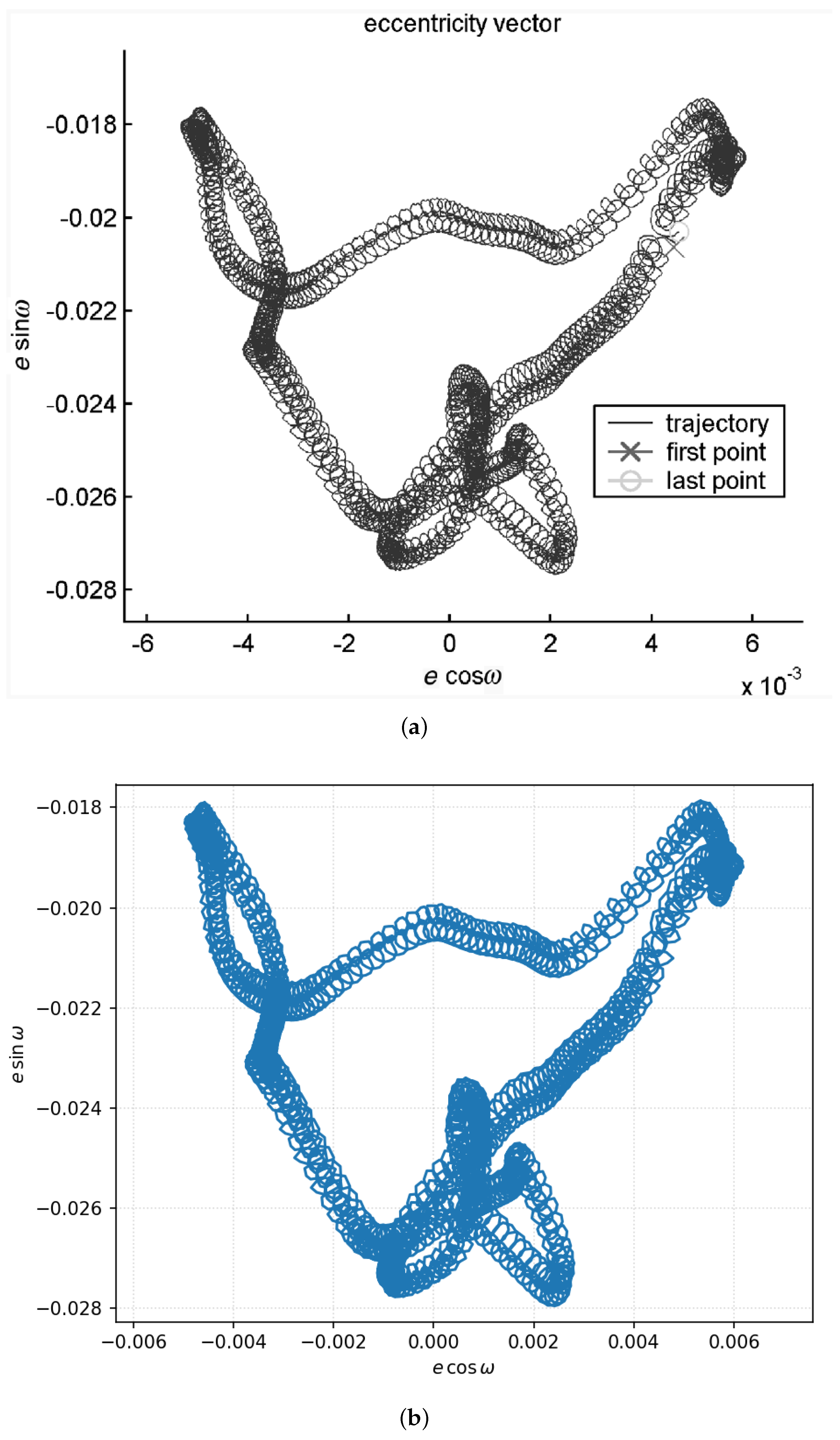
To validate the suggested two-stage procedure of frozen orbit design, we performed a lot of numerical experiments for various orbital plane orientations in space and different reference altitudes. Particularly, we have reproduced two repeat ground track orbits (RGT) from the paper of Russell and Lara [21]. The eccentricity vector evolution for two RGTs, medium ($h\approx 3308$ km) and low ($h\approx 124$ km), drawn in that paper (reprinted for convenience in Figure 3a and Figure 4a), very closely matches—almost coincides—with what is observed in our simulations (see Figure 3b and Figure 4b, respectively).

We also confirmed that for all the orbits we constructed, the eccentricity remains safely bounded even over a longer time interval (10 years) than was used during the optimization (1 year). This holds true within a more comprehensive dynamical model that now accounts for perturbations from Mercury, Venus, Mars, Jupiter, Saturn, Uranus, and Neptune, as well as lunar gravitational potential harmonics up to the 50th degree and order. Figure 5 and Figure 6 present polar plots illustrating the evolution of eccentricity and argument of periapsis for orbits at altitudes of 522 km and 261 km, both with a RAAN set to 0 degrees. Note that for the 522 km orbit, a collision with the Moon would occur at an eccentricity value of $e\approx 0.12$, and for the 261 km orbit, $e\approx 0.07$. As shown in the figures, the maximum eccentricity attained over 10 years is approximately 0.01 for both orbits.

Once a set of frozen orbits uniformly distributed around the Moon is obtained, initial states for same-plane satellites in a constellation may be assigned as states along the reference frozen orbit equidistant in time over the nominal orbital period.

A remark should be made that for a lunar orbiter, its elements are usually given with respect to the mean-Earth/mean-rotation (MER) reference frame which is employed to define the selenographic coordinates. At the same time, the spherical harmonic expansion of the lunar potential is given with respect to the so called Principal Axes (PA) reference frame. Its axes are very close to those of MER. The rotation matrix for the MER–PA transformation can be found in [10]. As for the PA–SCRF transformation, its matrix can be constructed using lunar libration angles included in the ephemeris information.

4. Constellation Design and Performance Metrics

The preliminary step in the design of frozen LLO constellations is to select an orbital configuration that we subsequently attempt to make frozen. In this study, we restrict ourselves to Walker–Mozhaev symmetric constellations in identical circular orbits distributed uniformly around the Moon. Four major parameters are to be defined for such a constellation:

• N, the total number of satellites;
• P, the number of orbital planes;
• $h_{\mathrm{ref}}$, the reference altitude of orbits in all the planes;
• F, the phase shift (in pattern units) between the respective satellites in adjacent planes.

Recall that the pattern unit $PU={360}^{\circ }/N$ was introduced by Walker ([25], p. 7) as a convenient unit to characterize the geometric pattern of a symmetric constellation. Without loss of generality, only values between 0 and $P-1$ can be considered for the phase shift because any other value of F describes the same pattern as $FmodP$. Moreover, for near-polar constellations, the F and $P-F$ patterns are almost identical ([25], p. 20). The zero shift is almost never applied due to its inferior coverage and collision safety properties. Thus, for two-plane and three-plane constellations, only the case of $F=1$ is worth being considered. For four-plane and five-plane constellations, patterns with $F=1$ and $F=2$ are to be studied, but we did not observe any significant difference between the performance characteristics of these options. So, using the standard notation $i^{\circ }:N/P/F$, we will further focus on ${84}^{\circ }:N/P/1$ constellations.

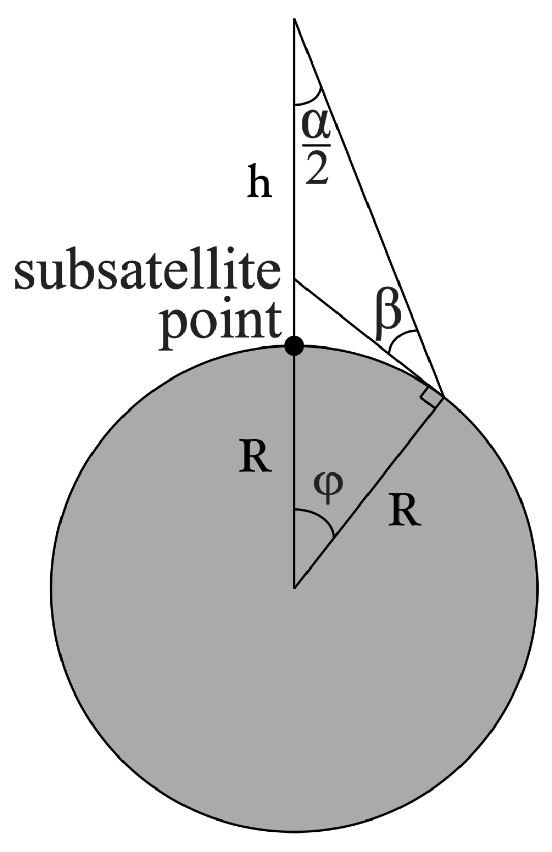
The design of symmetric constellations in identical circular orbits uniformly distributed around the spherical celestial body has been widely studied in a large number of papers since the pioneering works of Walker [25,26] and Mozhaev [27,28]. If a satellite orbits the body of radius R at altitude h, it covers the spot with the central half-angle $\phi$ (referred to as the footprint size in the below text) such that:

$$cos\beta ={\displaystyle \frac{R+h}{R}}sin{\displaystyle \frac{\alpha }{2}}={\displaystyle \frac{R+h}{R}}cos\left(\phi +\beta \right)$$

where $\beta$ is the minimum elevation angle at which an orbiting satellite is still considered visible (Figure 7).

Taking the value of $\beta =5^{\circ }$ typically adopted for atmosphereless bodies such as the Moon, we have:

$${\displaystyle \frac{h}{R}}={\displaystyle \frac{cos{5}^{\circ }}{cos\left({\phi }^{\circ }+5^{\circ }\right)}}-1$$

This gives a one-to-one correspondence between the orbital altitude and the footprint size.

The other quantities uniquely determined by the footprint size are the lower bound for the number of orbital planes:

$$P_{min}=⌈{\displaystyle \frac{{180}^{\circ }}{2{\phi }^{\circ }}}⌉$$

and the minimum number of satellites in each plane:

$${\left(N/P\right)}_{min}=⌈{\displaystyle \frac{{360}^{\circ }}{2{\phi }^{\circ }}}⌉$$

required for one-fold global continuous coverage. As for the total number of satellites in a single-coverage constellation, its static estimate from below:

$$N_{1f}=2+{\displaystyle \frac{{60}^{\circ }}{{60}^{\circ }-arctan\sqrt{3}cos\phi }}$$

is derived in the classical paper of Ballard [29]. Note that a simpler, but very close estimate can also be used:

$$N_{1f}\approx P_{min}·{\left(N/P\right)}_{min}=162·⌈{\left({\displaystyle \frac{{10}^{\circ }}{{\phi }^{\circ }}}\right)}^2⌉$$

The lower bound estimate for four-fold global continuous coverage by Walker–Mozhaev constellations is much harder to get analytically. To the best of our knowledge, it has not been published yet. The simplified estimate:

$$N_{4f}=4·N_{1f}$$

derived for street-of-coverage constellations is, therefore, utilized, despite such an estimate being slightly conservative for Walker–Mozhaev constellations.

In order to compactly and conveniently visualize basic constellation design parameters, we put forward the idea of a single Constellation Design (CoDe) nomogram, with the x-axis being the footprint size and the y-axis unified for the properly normalized four parameters (see Figure 8):

• Orbital altitude, expressed in a body’s radii;
• Free-space path loss (FSPL) of the signal power, normalized to its value at the altitude of $h=R$; it grows proportionally to the square of altitude;
• Minimum number of satellites in a constellation to provide 1-fold coverage (in hundreds);
• Minimum number of satellites in a constellation to provide 4-fold coverage (in hundreds).

Moreover, the green color shades of the background stripes indicate the corresponding number of orbital planes at least required, starting with two planes for the rightmost stripe.

The advantage of the developed nomogram is its universality (i.e., validity for any particular celestial body) and comprehensiveness, which makes it quite convenient for the preliminary constellation design.

Leveraging the CoDe nomogram, we selected two footprint sizes, $\phi ={25}^{\circ }$ and $\phi ={35}^{\circ }$, corresponding to the altitude values $h_{\mathrm{ref}}=0.15R_M\approx 261$ km and $h_{\mathrm{ref}}=0.3R_M\approx 522$ km, as potentially appropriate for candidate low-altitude lunar constellations: they ensure that the total number of satellites does not exceed 100 even for navigation purposes. As for the number of orbital planes, our analysis covers LLO constellations with at least two orbital planes, no matter which of the two reference altitude values is taken.

Among the performance metrics tracked, we are most interested in median and minimum numbers of visible spacecraft, globally and in lunar polar zones defined as North and South polar caps with latitudes higher than ${70}^{\circ }$. Additionally, the craters of Boguslawsky (72.9 S, 43.2 E) and Manzinus (67.7 S, 26.8 E) were of specific interest to us as the primary and backup landing sites of Russia’s recently failed Luna 25 mission. The constellation geometry quality for navigation is often quantified by the position dilution of precision (PDOP), a useful scalar metric that reflects how the user equivalent range error (UERE) is amplified due to poor configuration of visible satellites to result in higher user position uncertainty. The 50% (median) and 95% PDOP levels are tracked for both the poles and the craters of interest.

To evaluate the abovementioned metrics, we use a quasi-uniform grid on the Moon’s surface, which is generated as an outcome of the numerical optimization procedure similar to the one introduced in [30]. Specifically, to generate a grid of n almost uniformly distributed points on the unit sphere, one can search for unit vectors ${\mathbf{r}}_i\in {\mathbb{R}}^3$, $i=1,\dots ,n$, which minimize the objective function:

$$J=\sum _{1\le i<j\le n}log{\displaystyle \frac{1}{|{\mathbf{r}}_i-{\mathbf{r}}_j|}}$$

For convenience, the first six vectors ${\mathbf{r}}_1$,…, ${\mathbf{r}}_6$ have been fixed to $(\pm 1,0,0)$, $(0,\pm 1,0)$, and $(0,0,\pm 1)$, the points on the MER frame axes, including North and South poles. Moreover, we fix ${\mathbf{r}}_7$ and ${\mathbf{r}}_8$ at positions of Boguslawsky and Manzinus craters. In this study, $n=1200$ is set. Unlike our previous paper [9], where the optimization problem was solved by MATLAB’s realization of the interior point algorithm, the trust-region interior point method from the Python SciPy library is exploited. The initial guess is generated as a three-dimensional Gaussian random vector of unit norm. The resulting grid is shown in Figure 9.

5. Candidate Constellations Performance and Stability

In the framework of this study, several dozens of LLO constellations have been examined based on the the databases of frozen orbits for $h_{\mathrm{ref}}=261$ km and $h_{\mathrm{ref}}=522$ km. The osculating elements of the frozen orbits designed are given in

Table 2. Osculating elements of $h_{\mathrm{ref}}=261$ km frozen low lunar orbits (1 January 2022).

${\mathit{i}}_0={84}^{\circ }$	${\mathit{a}}_0$, km	${\mathit{e}}_{\mathit{x},0}={\mathit{e}}_{0}cos{\mathit{\omega }}_0$	${\mathit{e}}_{\mathit{y},0}={\mathit{e}}_{0}sin{\mathit{\omega }}_0$	${\mathit{e}}_0$
${\mathrm{\Omega }}_0=0^{\circ }$	$1.9912026·{10}^3$	$-1.141·{10}^{-3}$	$-0.820·{10}^{-3}$	$1.405·{10}^{-3}$
${\mathrm{\Omega }}_0={12}^{\circ }$	$1.9995086·{10}^3$	$0.836·{10}^{-3}$	$-0.499·{10}^{-3}$	$9.732·{10}^{-4}$
${\mathrm{\Omega }}_0={24}^{\circ }$	$2.0054516·{10}^3$	$2.636·{10}^{-3}$	$-1.447·{10}^{-3}$	$3.007·{10}^{-3}$
${\mathrm{\Omega }}_0={36}^{\circ }$	$2.0098165·{10}^3$	$3.446·{10}^{-3}$	$-1.868·{10}^{-3}$	$3.919·{10}^{-3}$
${\mathrm{\Omega }}_0={48}^{\circ }$	$2.0047492·{10}^3$	$3.475·{10}^{-3}$	$-2.118·{10}^{-3}$	$4.070·{10}^{-3}$
${\mathrm{\Omega }}_0={60}^{\circ }$	$2.0117974·{10}^3$	$2.808·{10}^{-3}$	$-2.866·{10}^{-3}$	$4.013·{10}^{-3}$
${\mathrm{\Omega }}_0={72}^{\circ }$	$2.0007286·{10}^3$	$1.710·{10}^{-3}$	$-2.500·{10}^{-3}$	$3.028·{10}^{-3}$
${\mathrm{\Omega }}_0={84}^{\circ }$	$1.9873625·{10}^3$	$0.665·{10}^{-3}$	$-2.769·{10}^{-3}$	$2.848·{10}^{-3}$
${\mathrm{\Omega }}_0={96}^{\circ }$	$1.9895695·{10}^3$	$-0.484·{10}^{-3}$	$-2.896·{10}^{-3}$	$2.936·{10}^{-3}$
${\mathrm{\Omega }}_0={108}^{\circ }$	$2.0002396·{10}^3$	$-1.505·{10}^{-3}$	$-2.533·{10}^{-3}$	$2.946·{10}^{-3}$
${\mathrm{\Omega }}_0={120}^{\circ }$	$1.9941854·{10}^3$	$-1.850·{10}^{-3}$	$-1.834·{10}^{-3}$	$2.605·{10}^{-3}$
${\mathrm{\Omega }}_0={132}^{\circ }$	$2.0001873·{10}^3$	$-1.900·{10}^{-3}$	$-2.580·{10}^{-3}$	$3.204·{10}^{-3}$
${\mathrm{\Omega }}_0={144}^{\circ }$	$2.0041044·{10}^3$	$-1.794·{10}^{-3}$	$-4.295·{10}^{-3}$	$4.655·{10}^{-3}$
${\mathrm{\Omega }}_0={156}^{\circ }$	$2.0100986·{10}^3$	$-1.583·{10}^{-3}$	$-5.297·{10}^{-3}$	$5.528·{10}^{-3}$
${\mathrm{\Omega }}_0={168}^{\circ }$	$2.0118254·{10}^3$	$-1.327·{10}^{-3}$	$-5.318·{10}^{-3}$	$5.481·{10}^{-3}$
${\mathrm{\Omega }}_0={180}^{\circ }$	$2.0030425·{10}^3$	$-0.804·{10}^{-3}$	$-5.281·{10}^{-3}$	$5.342·{10}^{-3}$
${\mathrm{\Omega }}_0={192}^{\circ }$	$2.0067555·{10}^3$	$-0.504·{10}^{-3}$	$-5.593·{10}^{-3}$	$5.616·{10}^{-3}$
${\mathrm{\Omega }}_0={204}^{\circ }$	$2.0050135·{10}^3$	$-0.321·{10}^{-3}$	$-4.606·{10}^{-3}$	$4.618·{10}^{-3}$
${\mathrm{\Omega }}_0={216}^{\circ }$	$1.9968808·{10}^3$	$-0.201·{10}^{-3}$	$-4.211·{10}^{-3}$	$4.216·{10}^{-3}$
${\mathrm{\Omega }}_0={228}^{\circ }$	$2.0025210·{10}^3$	$-0.123·{10}^{-3}$	$-3.868·{10}^{-3}$	$3.870·{10}^{-3}$
${\mathrm{\Omega }}_0={240}^{\circ }$	$2.0045079·{10}^3$	$-0.539·{10}^{-3}$	$-3.674·{10}^{-3}$	$3.714·{10}^{-3}$
${\mathrm{\Omega }}_0={252}^{\circ }$	$2.0074426·{10}^3$	$-0.808·{10}^{-3}$	$-3.889·{10}^{-3}$	$3.972·{10}^{-3}$
${\mathrm{\Omega }}_0={264}^{\circ }$	$2.0050989·{10}^3$	$-1.432·{10}^{-3}$	$-3.415·{10}^{-3}$	$3.703·{10}^{-3}$
${\mathrm{\Omega }}_0={276}^{\circ }$	$2.0006485·{10}^3$	$-2.112·{10}^{-3}$	$-3.287·{10}^{-3}$	$3.907·{10}^{-3}$
${\mathrm{\Omega }}_0={288}^{\circ }$	$2.0020608·{10}^3$	$-2.907·{10}^{-3}$	$-3.678·{10}^{-3}$	$4.688·{10}^{-3}$
${\mathrm{\Omega }}_0={300}^{\circ }$	$1.9985005·{10}^3$	$-3.954·{10}^{-3}$	$-3.639·{10}^{-3}$	$5.374·{10}^{-3}$
${\mathrm{\Omega }}_0={312}^{\circ }$	$2.0021262·{10}^3$	$-4.877·{10}^{-3}$	$-2.965·{10}^{-3}$	$5.708·{10}^{-3}$
${\mathrm{\Omega }}_0={324}^{\circ }$	$1.9978077·{10}^3$	$-4.856·{10}^{-3}$	$-1.451·{10}^{-3}$	$5.068·{10}^{-3}$
${\mathrm{\Omega }}_0={336}^{\circ }$	$1.9993934·{10}^3$	$-3.611·{10}^{-3}$	$-0.905·{10}^{-3}$	$3.722·{10}^{-3}$
${\mathrm{\Omega }}_0={348}^{\circ }$	$2.0101965·{10}^3$	$-2.088·{10}^{-3}$	$-1.286·{10}^{-3}$	$2.452·{10}^{-3}$

and

Table 3. Osculating elements of $h_{\mathrm{ref}}=522$ km frozen low lunar orbits (1 January 2022).

${\mathit{i}}_0={84}^{\circ }$	${\mathit{a}}_0$, km	${\mathit{e}}_{\mathit{x},0}={\mathit{e}}_{0}cos{\mathit{\omega }}_0$	${\mathit{e}}_{\mathit{y},0}={\mathit{e}}_{0}sin{\mathit{\omega }}_0$	${\mathit{e}}_0$
${\mathrm{\Omega }}_0=0^{\circ }$	$2.2499702·{10}^3$	$-0.030·{10}^{-3}$	$-4.350·{10}^{-3}$	$4.350·{10}^{-3}$
${\mathrm{\Omega }}_0={30}^{\circ }$	$2.2843859·{10}^3$	$2.393·{10}^{-3}$	$-4.699·{10}^{-3}$	$5.273·{10}^{-3}$
${\mathrm{\Omega }}_0={60}^{\circ }$	$2.2763719·{10}^3$	$1.367·{10}^{-3}$	$-4.930·{10}^{-3}$	$5.116·{10}^{-3}$
${\mathrm{\Omega }}_0={90}^{\circ }$	$2.2815410·{10}^3$	$-0.398·{10}^{-3}$	$-4.882·{10}^{-3}$	$4.898·{10}^{-3}$
${\mathrm{\Omega }}_0={120}^{\circ }$	$2.2855638·{10}^3$	$-0.667·{10}^{-3}$	$-5.243·{10}^{-3}$	$5.285·{10}^{-3}$
${\mathrm{\Omega }}_0={150}^{\circ }$	$2.2730989·{10}^3$	$-0.508·{10}^{-3}$	$-7.620·{10}^{-3}$	$7.637·{10}^{-3}$
${\mathrm{\Omega }}_0={180}^{\circ }$	$2.2619806·{10}^3$	$-1.007·{10}^{-3}$	$-7.987·{10}^{-3}$	$8.050·{10}^{-3}$
${\mathrm{\Omega }}_0={210}^{\circ }$	$2.2754016·{10}^3$	$-1.054·{10}^{-3}$	$-6.466·{10}^{-3}$	$6.552·{10}^{-3}$
${\mathrm{\Omega }}_0={240}^{\circ }$	$2.2770071·{10}^3$	$-0.822·{10}^{-3}$	$-5.186·{10}^{-3}$	$5.251·{10}^{-3}$
${\mathrm{\Omega }}_0={270}^{\circ }$	$2.2745247·{10}^3$	$-1.467·{10}^{-3}$	$-5.062·{10}^{-3}$	$5.270·{10}^{-3}$
${\mathrm{\Omega }}_0={300}^{\circ }$	$2.2513188·{10}^3$	$-3.457·{10}^{-3}$	$-5.538·{10}^{-3}$	$6.529·{10}^{-3}$
${\mathrm{\Omega }}_0={330}^{\circ }$	$2.2462503·{10}^3$	$-3.356·{10}^{-3}$	$-4.365·{10}^{-3}$	$5.506·{10}^{-3}$

. The initial epoch is midnight, 1 January 2022.

Among the number of different designs, we will further focus only on five configurations that seem to be best suited for the goals of global or local lunar surface coverage of a multiplicity high enough to ensure communication and navigation services. To visualize the parameters of the selected constellations, the five star marks are displayed on the CoDe nomogram (see Figure 10), with the y-value for each of the marks being equal to the total number of satellites (in 100 s) and the labels next to the marks designating the numbers of orbital planes and satellites per plane.

Out of the five candidate constellations, three correspond to $h_{\mathrm{ref}}=261$ km, whereas the other two are designed for $h_{\mathrm{ref}}=522$ km. The major performance metrics of the candidate constellations are summarized in

Table 4. Coverage performance for the candidate constellations.

${\mathit{h}}_{\mathbf{ref}}=261$ km	${\mathit{N}}_{\mathbf{global}}$	${\mathit{N}}_{\mathbf{North}}$	${\mathit{N}}_{\mathbf{South}}$	${\mathit{N}}_{\mathbf{Bogus}}$	${\mathbf{PDOP}}_{\mathbf{Npole}}$	${\mathbf{PDOP}}_{\mathbf{Spole}}$	${\mathbf{PDOP}}_{\mathbf{Bogus}}$
${84}^{\circ }:18/2/1$ $d_{min}=1.01$ km	min 0 med 0	min 1 med 2	min 1 med 2	min 1 med 2	N/A	N/A	N/A
${84}^{\circ }:54/3/1$ $d_{min}=0.37$ km	min 0 med 2	min 4 med 7	min 4 med 6	min 4 med 6	95% 6.5 med 2.0	95% 6.9 med 2.1	95% 10.9 med 3.0
${84}^{\circ }:70/5/1$ $d_{min}=0.54$ km	min 1 med 3	min 4 med 9	min 4 med 8	min 4 med 8	95% 3.2 med  1.9	95% 3.4 med  2.0	95% 4.8 med  2.4
${\mathit{h}}_{\mathbf{ref}}=\mathbf{522}$ km	${\mathit{N}}_{\mathbf{global}}$	${\mathit{N}}_{\mathbf{North}}$	${\mathit{N}}_{\mathbf{South}}$	${\mathit{N}}_{\mathbf{Bogus}}$	${\mathbf{PDOP}}_{\mathbf{Npole}}$	${\mathbf{PDOP}}_{\mathbf{Spole}}$	${\mathbf{PDOP}}_{\mathbf{Bogus}}$
${84}^{\circ }:36/3/1$ $d_{min}=2.66$ km	min  1 med 3	min  5 med 7	min  5 med 6	min  5 med 6	95%  7.2 med  1.8	95%  7.4 med  1.8	95%   8.2 med   2.3
${84}^{\circ }:99/3/1$ $d_{min}=1.30$ km	min  4 med 7	min  16 med 19	min  15 med 18	min  16 med 18	95%  1.1 med  1.0	95%  1.1 med  1.0	95%   1.5 med   1.2

. Note that the minumum distance between the constellation satellites is also tracked in addition to earlier mentioned metrics since it is a key safety parameter.

Based on the obtained results, one can conclude that three constellations (${84}^{\circ }:54/3/1$, ${84}^{\circ }:70/5/1$, ${84}^{\circ }:36/3/1$) are capable of providing navigation for the lunar polar zones, including the targeted craters and the poles themselves. Navigation quality is very good almost all the time. It is especially true for the ${84}^{\circ }:70/5/1$ constellation. Apart from high-precision polar navigation, it also provides the global communication service. The same property is shared by the ${84}^{\circ }:36/3/1$ constellation. Close performance can also be attained with significantly smaller numbers of satellites and orbital planes, but at the cost of four times higher FSPL due to the doubled altitude. In general, however, the larger the orbital altitude, the greater the minimum intersatellite distance and the safer the mission. So, performance and safety dictate the altitude to be as high as the satellite power budget allows.

The one-year evolution of the eccentricity vector and the semimajor axis for each orbital plane of the three constellations is shown in Figure 11, Figure 12 and Figure 13. To avoid overlapping, we displayed the curves for just one satellite in each orbital plane; the other satellites in the same plane have a very similar evolution. The figures confirm that all the constellation orbits are indeed frozen and remain near-circular. Note that a slight variation in the semimajor axis from plane to plane serves as the main instrument for meeting the frozenness condition.

If one seeks guaranteed navigation globally, over the entire lunar surface, the constellation size has to be significantly larger. For a three-plane design of the 522 km constellation, the number of satellites in each plane should be increased almost threefold: the ${84}^{\circ }:99/3/1$ constellation is the first attaining global continuous coverage.

On the other part of the range, among the downsized constellations, the ${84}^{\circ }:18/2/1$ constellation at a 261 km altitude seems to be the most promising if a continuous up/downlink for the lunar base in the polar region is required. There are no other lunar constellations orbiting so low that can perform more efficiently.

We should remark that the conducted analysis is not an exhaustive search for those LLO constellations that can be made frozen for a long time and also possess good performance metrics for lunar communication and navigation. The numerical results play an illustrative role to demonstrate opportunities the proposed techniques and tools provide to a mission designer.

It was interesting to reveal that, though the frozen LLOs seem to be long-term stable, they are actually unstable, though very mildly so. This instability, induced by the complex effect of lunar gravitational harmonics, can be proved based on the positive sign of the maximum Lyapunov characteristic exponent. Specifically, we estimate the leading finite-time Lyapunov exponent (FTLE):

$$\lambda \left(t;t_0\right)={\displaystyle \frac{ln\parallel \mathrm{\Phi }(t;t_0){\parallel }_2}{t-t_0}}$$

by integrating the variational equations for the state transition matrix $\mathrm{\Phi }(t;t_0)$ alongside the equations of motion (${\parallel ·\parallel }_2$ is the spectral norm of matrix). When we start increasing the propagation interval, the leading FTLE tends to some limit value. For the set of frozen orbits with $h_{\mathrm{ref}}=261$ km, this value appears to equal $3.5\times {10}^{-4}$ and almost does not depend on a specific orbit. In the case of $h_{\mathrm{ref}}=522$ km, the result is similar: $3\times {10}^{-4}$. Converting it to dimensional time units and inverting yields the characteristic instability time (Lyapunov time) of 1.1 to 1.3 months. According to existing studies of spacecraft motion in the unstable dynamical environment, the instability time provides us with a good estimate for the optimal frequency of impulsive station-keeping burns [31] or optimal update time for low-thrust orbit control [32]. This implies that the optimal periodicity of frozen orbit corrections is about once per month.

Using the same dynamical model parameters as those employed in the design of the frozen orbits (see Section 2), the numerical simulation of the station-keeping process for a typical frozen LLO has shown that a simple two-impulse correction maneuver works fairly well (see Figure 14), with the associated cost being on average from 10 to 30 m/s for different navigation uncertainty levels. Such an estimate correlates well with the 150 m/s annual station-keeping budget allocated for the Lunar Reconnaissance Orbiter mission [33]. The future extension of this work may include the results of Monte Carlo experiments to confirm the feasibility of long-term station keeping of frozen constellations.

6. Conclusions

The toolkit of techniques and instruments has been presented for the easy and robust design of frozen low lunar orbits and constellations employing such orbits. The Bayesian/Nelder–Mead non-gradient optimization method allows flexibly incorporating different orbit design constraints and at the same time succeeds in satisfying the frozenness condition with high accuracy. The novel compact nomogram, specially developed to visualize the preliminary design of Walker–Mozhaev constellations, has given useful insights regarding geometric configurations capable of providing the lunar surface coverage. The numerical study of different constellation designs has revealed several promising options for the deployment of navigation infrastructure in polar regions of the Moon, which are also applicable to the task of global communication. The Lyapunov time estimated for all the considered frozen low orbits shows weak instability, which requires small orbital corrections on a monthly basis.