
A Comparative Study of Airfoil Stall Characteristics Based on Detached Eddy Simulation Incorporated with Weighted Essentially Non-Oscillatory Scheme and Weighted Compact Nonlinear Scheme

Abstract
1. Introduction
2. Turbulence Model and Numerical Method
2.1. Turbulent Model
2.2. Numerical Method
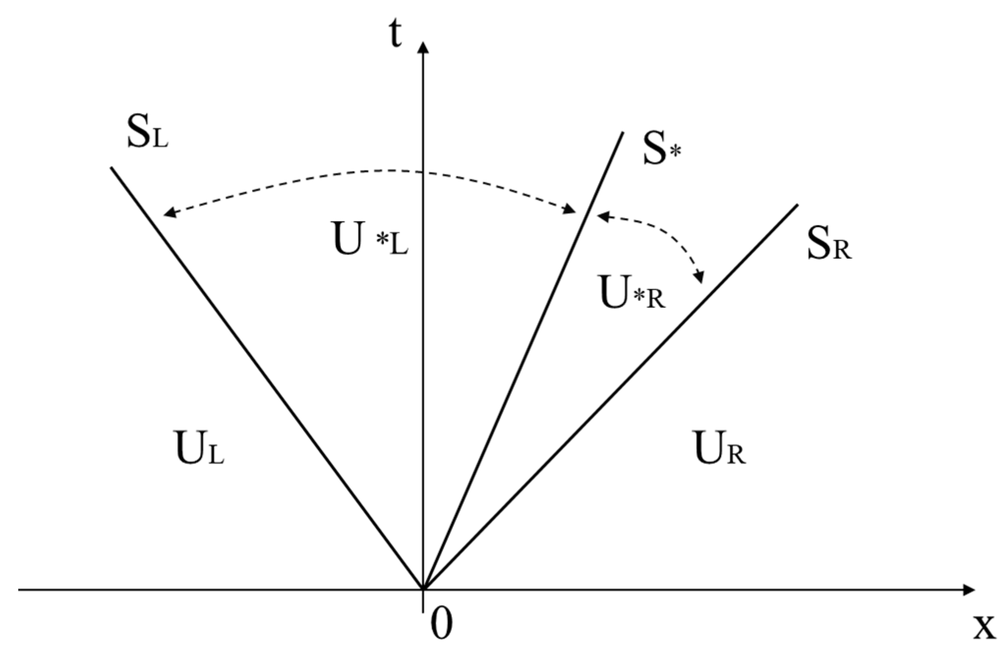
2.2.1. HLLC Scheme
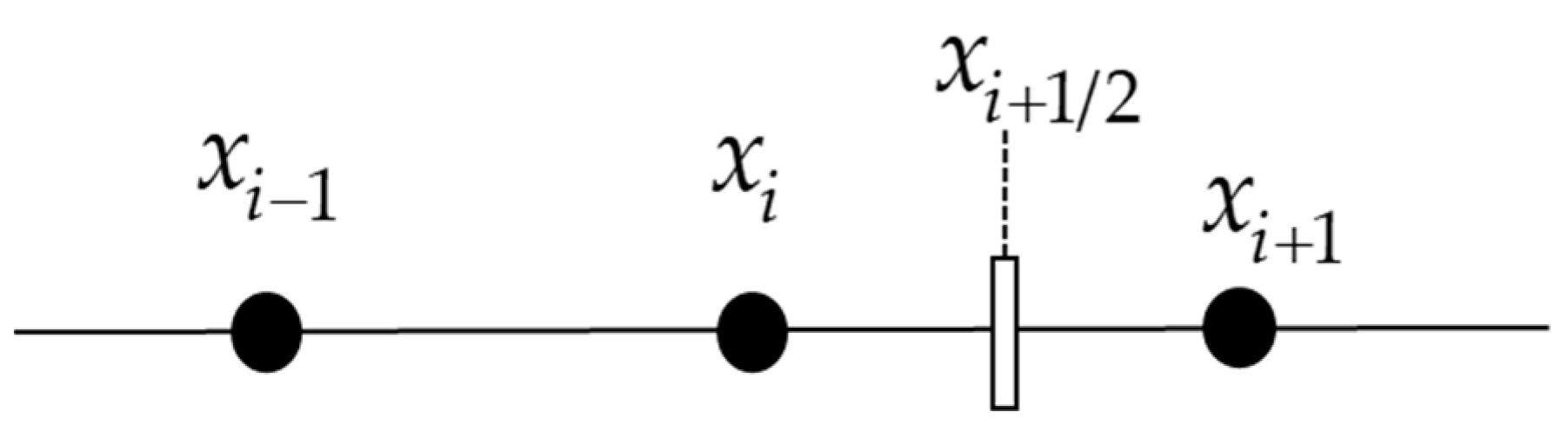
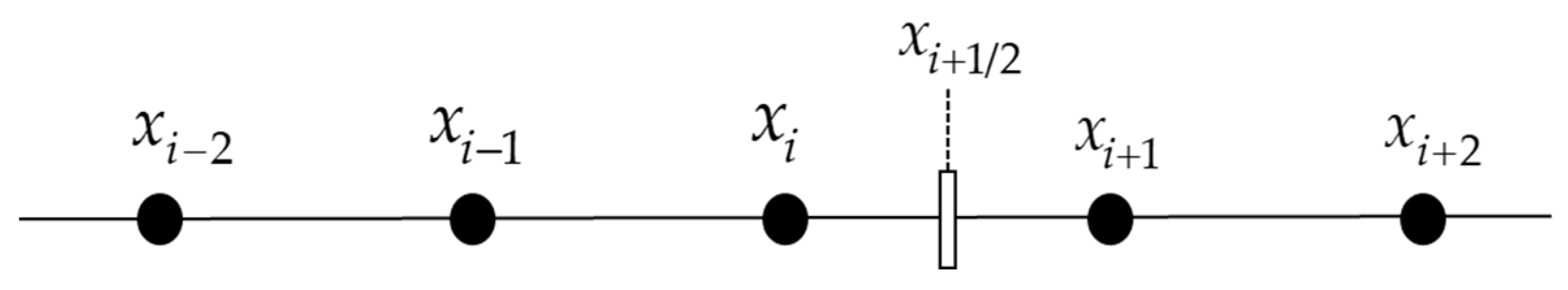
2.2.2. WCNS
2.3. Time-Marching Scheme
3. Numerical Simulation Results and Discussion
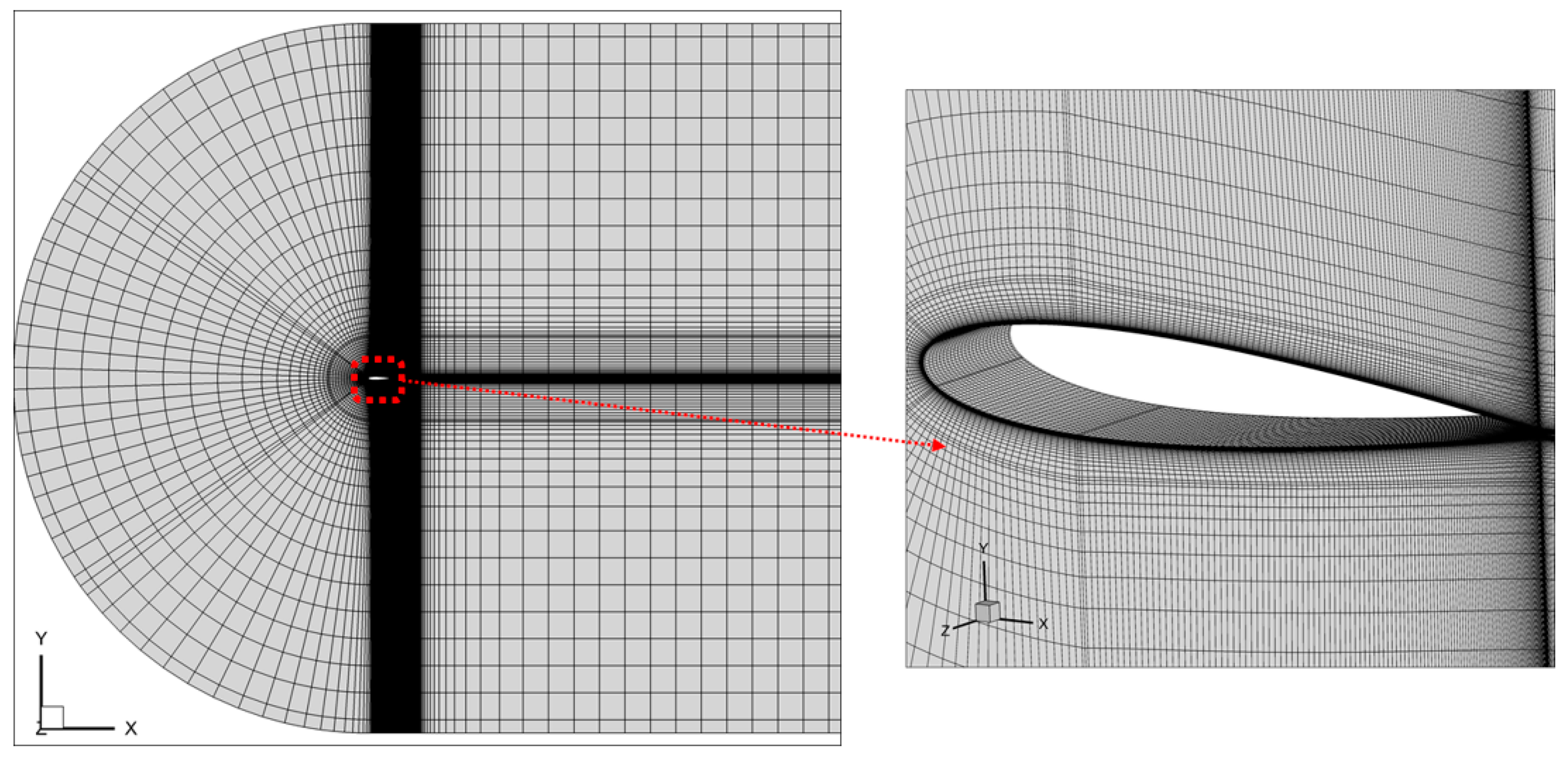
3.1. Mesh Subdivision
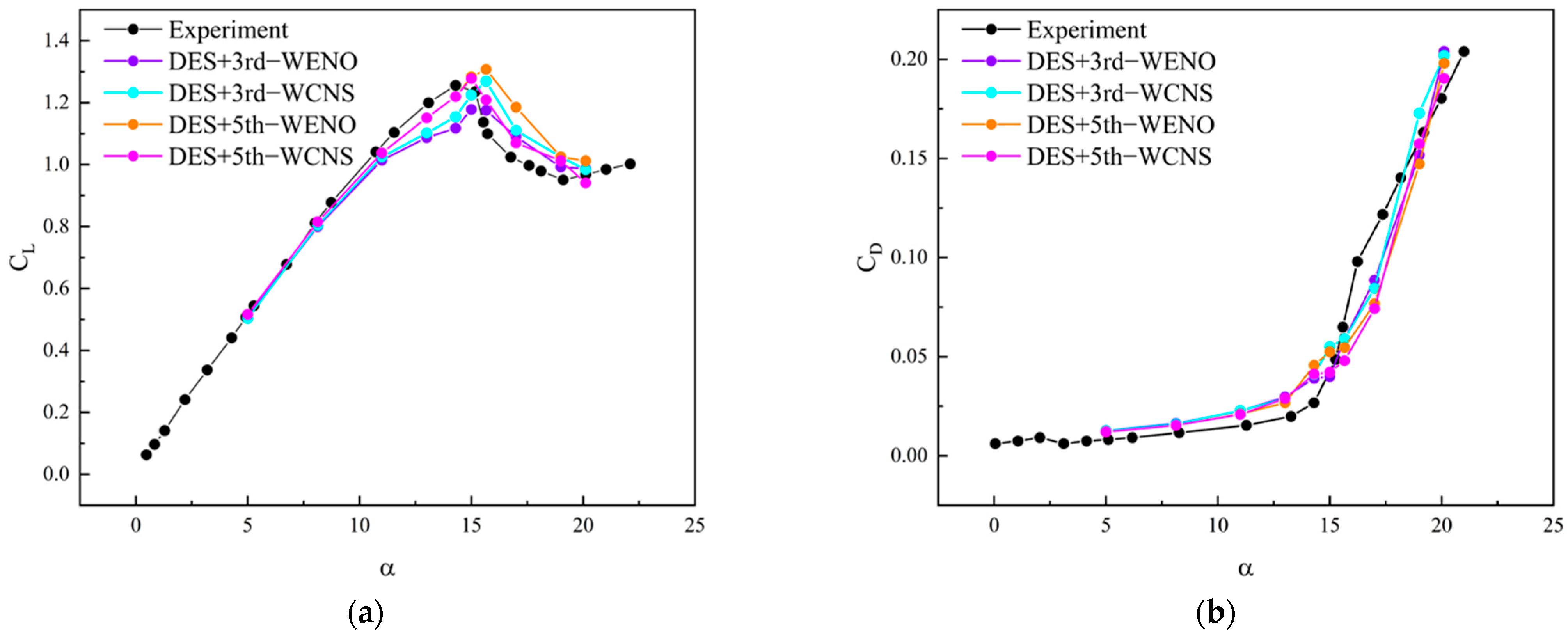
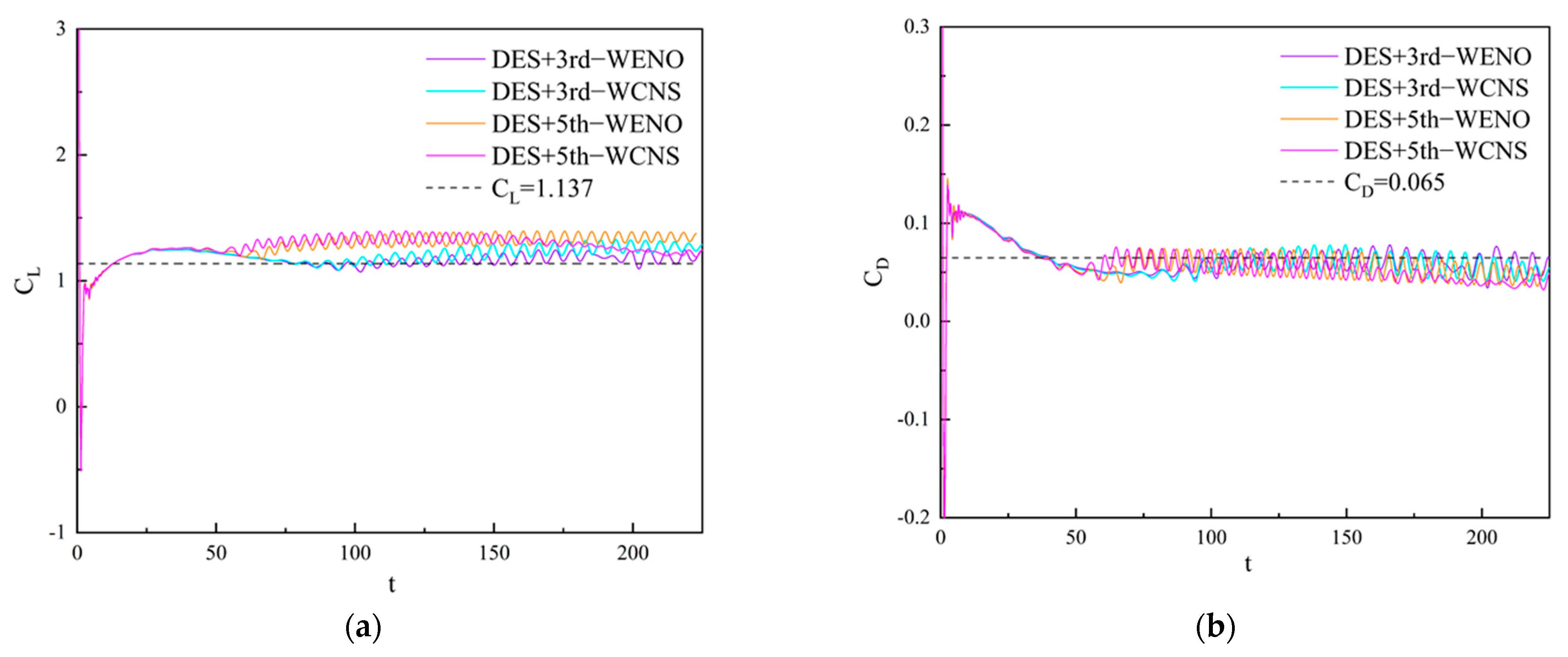
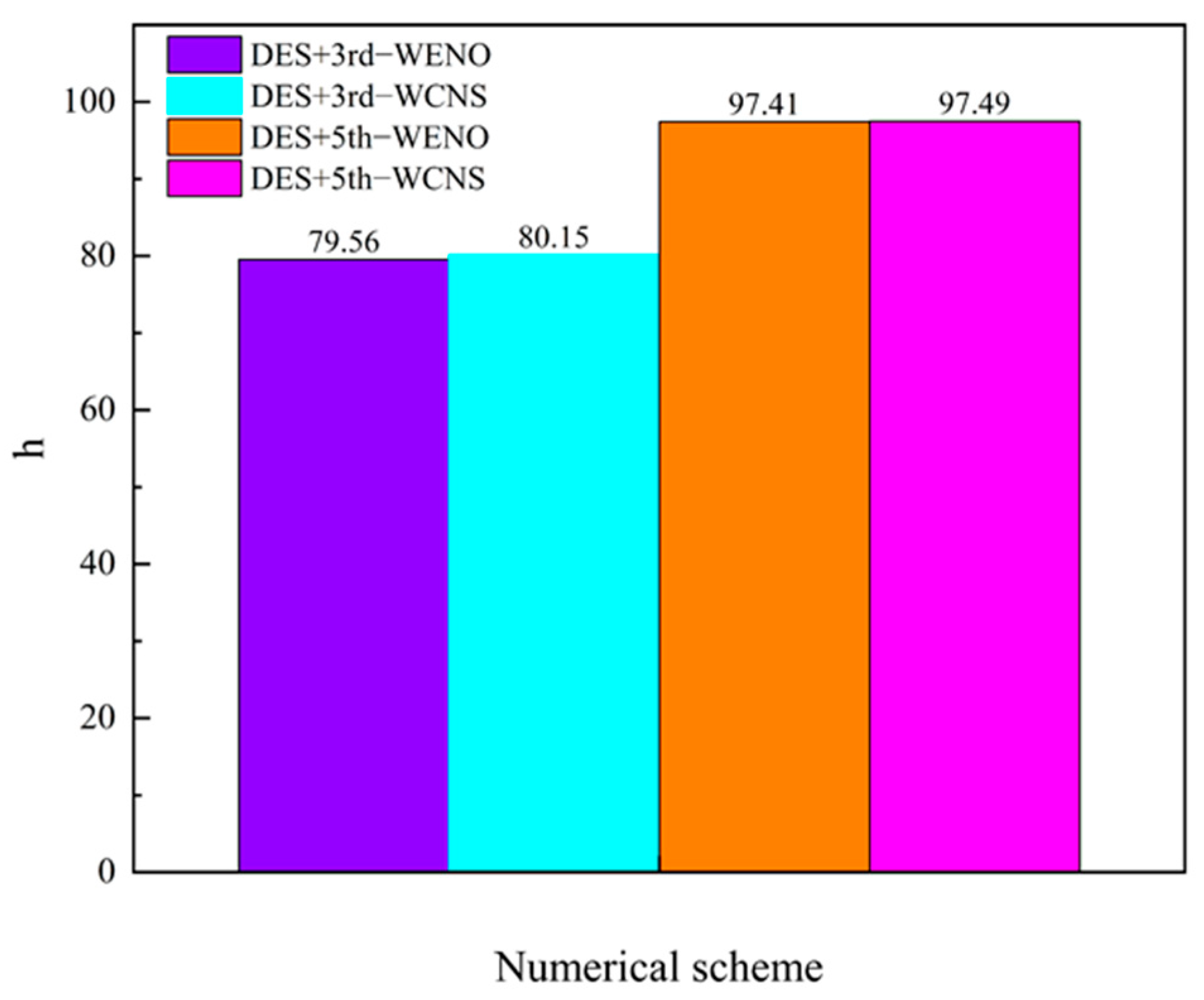
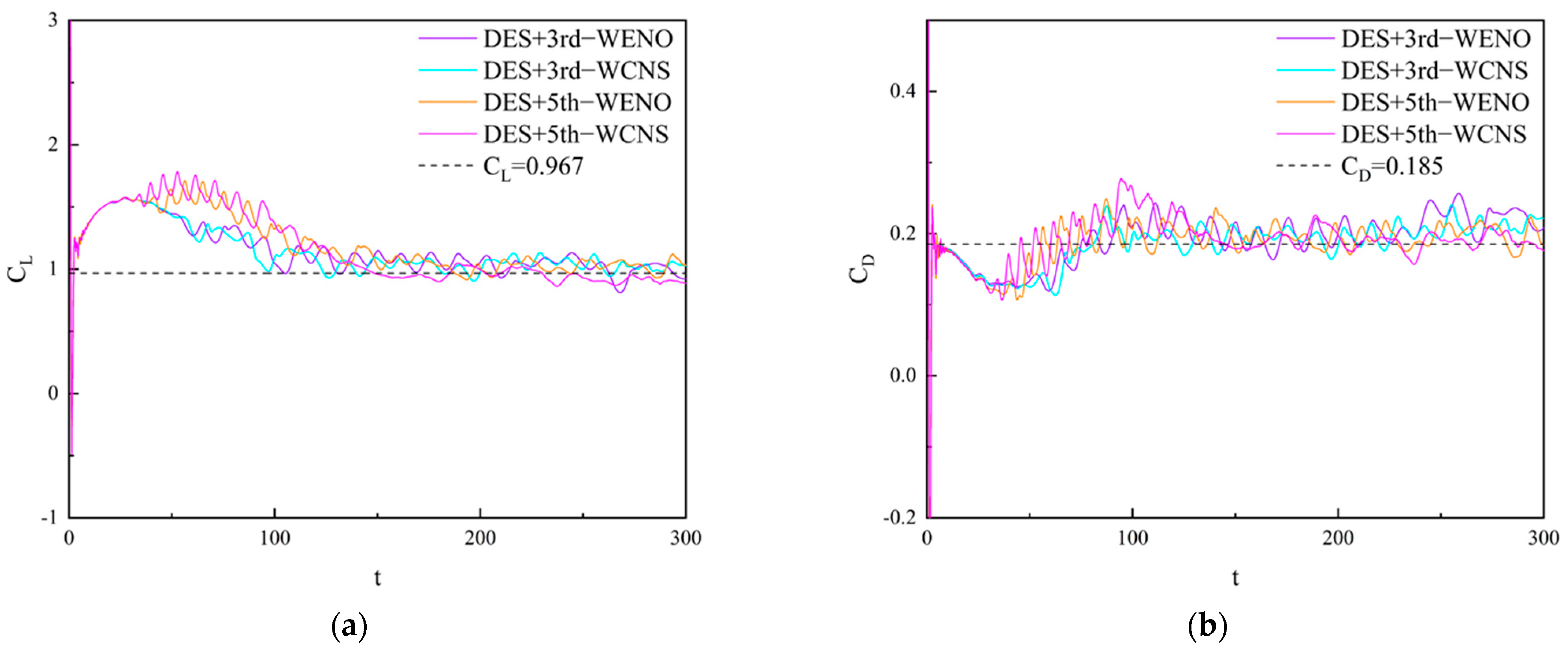
3.2. Analysis of Time-Average Results
3.3. Instantaneous Flow Field Analysis
4. Conclusions
Author Contributions
Funding
Data Availability Statement
Conflicts of Interest
References
- Mani, M.; Dorgan, A.J. A perspective on the state of aerospace computational fluid dynamics technology. Annu. Rev. Fluid Mech. 2023, 55, 431–457. [Google Scholar] [CrossRef]
- Slotnick, J.P.; Khodadoust, A.; Alonso, J.; Darmofal, D.; Gropp, W.; Lurie, E.; Mavriplis, D.J. CFD Vision 2030 Study: A Path to Revolutionary Computational Aerosciences; NASA Contractor Report; NASA: Washington, DC, USA, 2013. [Google Scholar]
- Zhang, Z.S.; Cui, G.X.; Xu, C.X. Turbulence Theory and Simulation, 2nd ed.; Tsinghua University Press: Beijing, China, 2017; pp. 173–174. [Google Scholar]
- Spalart, P.R. Strategies for turbulence modelling and simulations. Int. J. Heat Fluid Flow 2000, 21, 252–263. [Google Scholar] [CrossRef]
- The, J.; Yu, H.S. A Critical Review on the Simulations of Wind Turbine Aerodynamics Focusing on Hybrid RANS-LES Methods. Energy 2017, 138, 257–289. [Google Scholar] [CrossRef]
- Spalart, P.R.; Jou, W.H.; Strelets, M. Comments on the feasibility of LES for wings and on a hybrid RANS/LES approach. In Proceedings of the 1st AFOSR International Conference on DNS/LES, Advances in DNS/LES, Ruston, LA, USA, 4–8 August 1997; Grey den Press: Columbus, OH, USA, 1997. [Google Scholar]
- Strelets, M. Detached eddy simulation of massively separated flows. In Proceedings of the 39th Aerospace Sciences Meeting and Exhibit, Reno, NV, USA, 8–11 January 2001; p. 879. [Google Scholar] [CrossRef]
- Spalart, P.R. Detached-eddy simulation. Annu. Rev. Fluid Mech. 2009, 41, 181–202. [Google Scholar] [CrossRef]
- Menter, F.R.; Kuntz, M.; Langtry, R. Ten years of industrial experience with the SST turbulence model. Turbul. Heat Mass Transf. 2003, 4, 625–632. [Google Scholar]
- Spalart, P.R.; Deck, S.; Shur, M.L.; Squires, K.D.; Strelets, M.K.; Travin, A. A new version of detached-eddy simulation, resistant to ambiguous grid densities. Theor. Comput. Fluid Dyn. 2006, 20, 181–195. [Google Scholar] [CrossRef]
- Liu, X.D.; Osher, S.; Chan, T. Weighted essentially non-oscillatory schemes. J. Comput. Phys. 1994, 115, 200–212. [Google Scholar] [CrossRef]
- Jiang, G.S.; Shu, C.W. Efficient implementation of weighted ENO schemes. J. Comput. Phys. 1996, 126, 202–228. [Google Scholar] [CrossRef]
- Lele, S.K. Compact finite difference schemes with spectral-like resolution. J. Comput. Phys. 1992, 103, 16–42. [Google Scholar] [CrossRef]
- Deng, X.; Zhang, H. Developing high-order weighted compact nonlinear schemes. J. Comput. Phys. 2000, 165, 22–44. [Google Scholar] [CrossRef]
- Deng, X.; Mao, M.; Liu, J. High-order dissipative weighted compact nonlinear schemes for Euler and Navier-Stokes equations. In Proceedings of the 15th AIAA Computational Fluid Dynamics Conference, Anaheim, CA, USA, 11–14 June 2001; p. 2626. [Google Scholar] [CrossRef]
- Zhang, X.; Chen, X.; Jiang, Y. Comparison Study of the Fifth-Order WCNS and WENO Scheme In the Truncation Error, Dissipation and Dispersion Terms. J. Phys. Conf. Ser. 2021, 1865, 022003. [Google Scholar] [CrossRef]
- Nonomura, T.; Iizuka, N.; Fujii, K. Freestream and vortex preservation properties of high-order WENO and WCNS on curvilinear grids. Comput. Fluids 2010, 39, 197–214. [Google Scholar] [CrossRef]
- Kamiya, T.; Asahara, M.; Nonomura, T. Effect of flux evaluation methods on the resolution and robustness of the two-step finite-difference WENO scheme. Numer. Math. 2020, 13, 1068–1097. [Google Scholar] [CrossRef]
- Ge, M.M. Large Eddy Simulation Based on WCNS Scheme and Its Application in Aeroacoustics. Ph.D. Thesis, National University of Defense Technology, Changsha, China, 2020. [Google Scholar]
- Toro, E.F.; Spruce, M.; Speares, W. Restoration of the contact surface in the HLL-Riemann solver. Shock. Waves 1994, 4, 25–34. [Google Scholar] [CrossRef]
- Spalart, P.; Allmaras, S. A one-equation turbulence model for aerodynamic flows. In Proceedings of the 30th Aerospace Sciences Meeting and Exhibit, Reno, NV, USA, 6–9 January 1992. [Google Scholar] [CrossRef]
- Harten, A.; Lax, P.D.; Leer, B.V. On upstream differencing and Godunov-type schemes for hyperbolic conservation laws. SIAM Rev. 1983, 25, 35–61. [Google Scholar] [CrossRef]
- Niu, Y.Y.; Chang, C.H.; Tseng, W.Y.I.; Peng, H.H.; Yu, H.Y. Numerical simulation of an aortic flow based on a hllc type incompressible flow solver. Commun. Comput. Phys. 2009, 5, 142. [Google Scholar]
- Nichols, R.; Tramel, R.; Buning, P. Solver and turbulence model upgrades to OVERFLOW 2 for unsteady and high-speed applications. In Proceedings of the 24th AIAA Applied Aerodynamics Conference, San Francisco, CA, USA, 5–8 June 2006; p. 2824. [Google Scholar] [CrossRef]
- Butcher, J.C. On Runge-Kutta processes of high order. J. Aust. Math. Society 1964, 4, 179–194. [Google Scholar] [CrossRef]
- Klopfer, G.; Hung, C.; Van der Wijngaart, R.; Onufer, J. A diagonalized diagonal dominant alternating direction implicit (D3ADI) scheme and subiteration correction. In Proceedings of the 29th AIAA, Fluid Dynamics Conference, Albuquerque, NM, USA, 15–18 June 1998; p. 2824. [Google Scholar] [CrossRef]
- Yoon, S.; Jameson, A. Lower-upper symmetric-Gauss-Seidel method for the Euler and Navier-Stokes equations. AIAA J. 1988, 26, 1025–1026. [Google Scholar] [CrossRef]
- Bertagnolio, F. NACA0015 Measurements in LM Wind Tunnel and Turbulence Generated Noise; Technical University of Denmark: Roskilde, Denmark, 2008. [Google Scholar]


Disclaimer/Publisher’s Note: The statements, opinions and data contained in all publications are solely those of the individual author(s) and contributor(s) and not of MDPI and/or the editor(s). MDPI and/or the editor(s) disclaim responsibility for any injury to people or property resulting from any ideas, methods, instructions or products referred to in the content. |
© 2024 by the authors. Licensee MDPI, Basel, Switzerland. This article is an open access article distributed under the terms and conditions of the Creative Commons Attribution (CC BY) license (https://creativecommons.org/licenses/by/4.0/).
Share and Cite
Qi, Y.; Zhong, B.; Zou, S. A Comparative Study of Airfoil Stall Characteristics Based on Detached Eddy Simulation Incorporated with Weighted Essentially Non-Oscillatory Scheme and Weighted Compact Nonlinear Scheme. Aerospace 2024, 11, 917. https://doi.org/10.3390/aerospace11110917
Qi Y, Zhong B, Zou S. A Comparative Study of Airfoil Stall Characteristics Based on Detached Eddy Simulation Incorporated with Weighted Essentially Non-Oscillatory Scheme and Weighted Compact Nonlinear Scheme. Aerospace. 2024; 11(11):917. https://doi.org/10.3390/aerospace11110917
Chicago/Turabian StyleQi, Yan, Bowen Zhong, and Song Zou. 2024. "A Comparative Study of Airfoil Stall Characteristics Based on Detached Eddy Simulation Incorporated with Weighted Essentially Non-Oscillatory Scheme and Weighted Compact Nonlinear Scheme" Aerospace 11, no. 11: 917. https://doi.org/10.3390/aerospace11110917
APA StyleQi, Y., Zhong, B., & Zou, S. (2024). A Comparative Study of Airfoil Stall Characteristics Based on Detached Eddy Simulation Incorporated with Weighted Essentially Non-Oscillatory Scheme and Weighted Compact Nonlinear Scheme. Aerospace, 11(11), 917. https://doi.org/10.3390/aerospace11110917