Ballistic Fitting Impact Point Prediction Based on Improved Crayfish Optimization Algorithm

Abstract

To solve the problem of difficulty in predicting the impact point clearly and promptly during projectile flight, this paper proposes an improved ballistic-impact-point prediction method. A certain type of high-spinning tailed projectile is taken as the research object for online real-time landing point prediction research. This study comprehensively utilizes the real-time radar measurement data and the geomagnetic data measured by the bomb-carried geomagnetic sensor. It applies the four-degree-of-freedom ballistic model to predict the landing point. First, the roll angular velocity is calculated based on the geomagnetic data, after which the radar real-time measurement data are segmentally fitted using the improved crayfish algorithm. Then, the fitted parameters are substituted into the four-degree-of-freedom ballistic model. Finally, the C-K method is used to identify the aerodynamic parameters, and the identified aerodynamic parameters are used for fallout prediction. The simulation results show a small deviation between the predicted and actual impact points using the improved ballistic-impact-point prediction method.

1. Introduction

In modern warfare, mortars, howitzers, rockets, and other types of artillery still play an important role in modern conventional warfare, with all types of projectiles as the object of combat artillery reconnaissance radar, which is also in constant development [1,2,3,4]. The ballistic extrapolation algorithms of traditional gun position surveillance and calibration radars are mostly based on the projectile motion model, and the projectile motion parameters are calculated through Kalman filtering to predict the impact point [5,6,7,8]. For example, the common method is to analyze and predict the flight trajectory of the projectile using the classical mechanical model combined with the filtering algorithm. To a certain extent, this method can meet the basic combat requirements. However, with the increasingly complex war environment and the continuous improvement of the requirements for accuracy, its limitations have gradually emerged.

In recent years, with the development of artificial intelligence and machine learning technologies, some new algorithms have been applied in the field of projectile-impact-point prediction. For instance, Zhao and Lei et al. [9] proposed a modified algorithm for a projectile long-duration fallout prediction model based on a long–short-term memory (LSTM) network, which adopts the traditional untraceable Kalman filter (UKF) method as the priori knowledge base and combines with the modified prediction model of the LSTM network to predict the fallout of the projectile. Lu and Qi et al. [10] used the range and transverse deviation as sequence data to establish the LSTM fallout prediction network model to predict the projectile fallout. Tian and Duan et al. [11] established nonlinear mapping models, such as support vector regression machine, BP neural network, and genetic algorithm optimization LSSVM from initial speed radar to continuous wave radar, and then combined the predicted values of the four models to calculate the predicted values of the combined model’s fallout point. Wei and Huo [12] proposed a ballistic fallout prediction method based on the unscented Kalman filter algorithm. These methods have improved the accuracy and adaptability of impact point prediction to varying degrees, but they still face some challenges in practical applications.

Although the existing methods have achieved certain results, when the radar measurement data is messy during the actual flight process, they still have some shortcomings. On the one hand, the projectile encounters various noise interferences during the flight process, including the noises generated by the projectile’s own motion, air friction, and external environment. These noises affect the accuracy and stability of the radar measurement data, causing the traditional model-based and filtering-based methods to accumulate errors when dealing with these messy data, thereby reducing the accuracy of impact point prediction. On the other hand, the complex and changeable meteorological conditions, such as the changes in wind direction and speed, fluctuations in air pressure, and differences in temperature, have a significant impact on the flight trajectory of the projectile [13,14]. However, the existing methods have limited capabilities in dealing with the real-time changes and uncertainties of these meteorological factors and it is difficult to accurately incorporate them into the prediction model, resulting in deviations between the prediction results and the actual impact points. The identification of aerodynamic parameters is of crucial importance in ballistic prediction, but the existing methods need to improve in terms of the accuracy and timeliness of aerodynamic parameter identification. Accurate aerodynamic parameters can precisely reflect the aerodynamic forces acting on the projectile during flight, directly affecting the accuracy of impact point prediction [15,16,17]. However, in actual situations, it is difficult to identify the aerodynamic parameters after the projectile passes through the ballistic vertex. Traditional methods may not be able to fully utilize all the ballistic data to mine the aerodynamic characteristics of the projectile’s flight, resulting in inaccurate identification of aerodynamic parameters, which in turn causes a large deviation between the four-degree-of-freedom ballistic model and the actual flight situation, unable to meet the high requirements of modern warfare for projectile shooting accuracy.

Based on the current status of the existing technical level and the existing gaps, in order to predict the ballistic impact point of the projectile more accurately and quickly, improve the shooting accuracy of the projectile, and meet the higher requirements of modern conventional warfare for the impact point prediction of gun position surveillance and calibration radars, this paper proposes a ballistic fitting impact point prediction method based on the improved crayfish algorithm. This method fits the radar measurement data using the improved crayfish algorithm, calculates the roll angular velocity based on the geomagnetic data, and then combines the C-K method to identify the aerodynamic parameters and substitutes them into the four-degree-of-freedom ballistic model to predict the impact point. The aim is to overcome the shortcomings of the existing methods when facing messy radar measurement data and complex flight environments, improve the accuracy and reliability of impact point prediction, and provide more effective support for artillery operations in modern warfare.

2. Projectile Motion Model

The projectile center of mass is subjected to several complex factors during its motion such as drag, lift, gravity, Koch inertial force, Magnus force, etc., which in turn are closely related to the parameters of the projectile’s attitude and rotation [18].

Compared to the six-degree-of-freedom model for impact point prediction, which is time-consuming, the four-degree-of-freedom model of a projectile is a commonly used model for describing the motion of a projectile. This model mainly considers four degrees of freedom of the projectile in space, including three translational degrees of freedom (corresponding to the position change of the projectile in the $x$, $y$, and $z$ directions, respectively) and one rotational degree of freedom (usually the angular velocity of the projectile’s roll). In this model, the motion of the projectile is subject to a variety of forces, and by constructing the corresponding dynamic equations, the trajectory and state changes of the projectile under the action of these forces can be more accurately described. Specifically, the four-degree-of-freedom model takes into account parameters such as the projectile’s position, velocity, acceleration, and roll angular velocity, and predicts the projectile’s point of impact by solving these parameters. The model has important application value in the design of projectiles, ballistic analysis, and fall point prediction. The four-degree-of-freedom model is shown below:

$$\left\{\begin{array}{l}{\displaystyle \frac{\mathrm{d}v}{\mathrm{d}t}}={\displaystyle \frac{1}{m}}{F}_{x_2}\\ {\displaystyle \frac{\mathrm{d}{\theta }_a}{\mathrm{d}t}}={\displaystyle \frac{1}{mv\cos {\psi }_2}}{F}_{y_2}\\ {\displaystyle \frac{\mathrm{d}{\psi }_2}{\mathrm{d}t}}={\displaystyle \frac{1}{mv}}{F}_{z_2}\\ {\displaystyle \frac{\mathrm{d}x}{\mathrm{d}t}}=v\cos {\psi }_2\cos {\theta }_a\\ {\displaystyle \frac{\mathrm{d}y}{\mathrm{d}t}}=v\cos {\psi }_2\sin {\theta }_a\\ {\displaystyle \frac{\mathrm{d}z}{\mathrm{d}t}}=v\sin {\psi }_2\\ {\displaystyle \frac{\mathrm{d}{\omega }_{xi}}{\mathrm{d}t}}={\displaystyle \frac{1}{C}}{M}_{\xi }\end{array}\right.$$

(1)

where $v$ refers to the flight speed of the projectile; ${\theta }_a$ refers to the velocity height angle (also known as ballistic inclination); ${\psi }_2$ refers to the velocity direction angle (also known as ballistic deflection); $x$, $y$, and $z$ refer to the center of mass of the projectile spatial coordinates (horizontal distance, ballistic height, side deviation); ${\omega }_{xi}$ refers to the angular velocity of the projectile roll; $F_{x_2}$, $F_{y_2}$, and $F_{z_2}$ refer to the action of the projectile all the combined force in the ballistic coordinate system of the three components; $M_{\xi }$ refers to the action of the projectile roll direction of the combined moment; $m$ refers to the mass of the projectile; and $C$ refers to the polar moment of inertia, equal to 0.14.

The expressions of $F_{x_2}$, $F_{y_2}$, $F_{z_2}$, and $M_{\xi }$ are given in Equations (2)–(5):

$$\begin{array}{l}{F}_{x_2}={\displaystyle \frac{-\rho v_{r}S}{2}}{c}_{x_0}(v-w_{x_2})-mg\sin {\theta }_a\cos {\psi }_2+\\ {\displaystyle \frac{\rho S}{2}}{c}_y{\displaystyle \frac{{\delta }_r}{\sin {\delta }_r}}(v_r^2\cos {\delta }_{2p}\cos {\delta }_{1p}-v_{r\xi }(v-w_{x_2}))\end{array}$$

(2)

$$\begin{array}{l}{F}_{y_2}={\displaystyle \frac{\rho v_{r}S}{2}}{c}_{x_0}{w}_{y_2}-mg\cos {\theta }_a+\\ {\displaystyle \frac{\rho S}{2}}{c}_y{\displaystyle \frac{{\delta }_r}{\sin {\delta }_r}}(v_r^2\cos {\delta }_{2p}\sin {\delta }_{1p})\end{array}$$

(3)

$$\begin{array}{l}{F}_{z_2}={\displaystyle \frac{\rho v_{r}S}{2}}{c}_{x_0}{w}_{z_2}+mg\sin {\theta }_a\sin {\psi }_2+\\ {\displaystyle \frac{\rho S}{2}}{c}_y{\displaystyle \frac{{\delta }_r}{\sin {\delta }_r}}{v}_r^2\sin {\delta }_{2p}\cos {\delta }_{1p}\end{array}$$

(4)

$$M_{\xi }=-{\displaystyle \frac{\rho SLd}{2}}{m}_{xz}{v}_r{w}_{xi}+{\displaystyle \frac{\rho v_r^2}{2}}SL{m}_{xw}{\delta }_f$$

(5)

where $\rho$ refers to the density; $S$ refers to the cross-sectional area of the projectile; $c_{x_0}$ refers to the drag coefficient; $g$ refers to the gravitational acceleration; $c_y$ refers to the derivative of the coefficient of lift; $m_{xz}$ refers to the derivative of the coefficient of the extreme damping moment; $m_{xw}$ refers to the derivative of the coefficient of the inverted moment of the tail; $d$ refers to the diameter of the projectile; $L$ refers to the length of the projectile; and ${\delta }_f$ refers to the tail mounting angle, which is 1°.

The expressions of $w_{x_2}$, $w_{y_2}$, $w_{z_2}$, $v_r$, ${\delta }_{2p}$, ${\delta }_{1p}$, $v_{r\xi }$, and ${\delta }_r$ in Equations (2)–(5) are shown below:

$$w_{x_2}=w_x\cos {\psi }_2\cos {\theta }_a+w_z\sin {\psi }_2$$

(6)

$$w_{y_2}=-w_x\sin {\theta }_a$$

(7)

$$w_{z_2}=-w_x\sin {\psi }_2\cos {\theta }_a+w_z\cos {\psi }_2$$

(8)

$$v_r=\sqrt{{(v-w_{x_2})}^2+w_{y2}^2+w_{z2}^2}$$

(9)

$${\delta }_{2p}=-{\displaystyle \frac{P}{Mv}}\stackrel{·}{\theta }$$

(10)

$${\delta }_{1p}=-{\displaystyle \frac{P^{2}T}{M^{2}v}}\stackrel{·}{\theta }$$

(11)

$$\begin{array}{l}{v}_{r\xi }=(v-w_{x_2})\cos {\delta }_{2p}\cos {\delta }_{1p}-w_{z_2}\sin {\delta }_{2p}\\ -w_{y_2}\cos {\delta }_{2p}\sin {\delta }_{1p}\end{array}$$

(12)

$${\delta }_r=\arccos (v_{r\xi }/v_r)$$

(13)

where the expressions of $w_x$, $w_z$, $\stackrel{·}{\theta }$, $P$, $M$, and $T$ are shown below:

$$w_x=-w\cos (a_W-a_N)$$

(14)

$$w_z=-w\sin (a_W-a_N)$$

(15)

$$\stackrel{·}{\theta }=-g\cos {\theta }_a/v$$

(16)

$$P={\displaystyle \frac{C{\omega }_{xi}}{Av}}$$

(17)

$$M={\displaystyle \frac{\rho SL}{2A}}{m}_z$$

(18)

$$T={\displaystyle \frac{\rho S}{2m}}{c}_y$$

(19)

where $w$ refers to the wind speed; $a_W$ refers to the wind direction; $a_N$ refers to the projectile direction; and $A$ refers to the equatorial moment of inertia, which is equal to 1.61.

To describe clearly and accurately each symbol involved in the process of projectile modeling and avoid confusion in the use of symbols, a nomenclature chart for projectile modeling (

Table 1. A table for the nomenclature used in the modeling of the ballistic projectile.

Symbol	Meaning
$v$, ${\theta }_a$, ${\psi }_2$	projectile velocity, velocity height angle, velocity direction angle
$x$, $y$, $z$	horizontal distance, ballistic height, side deviation
${\omega }_{xi}$	angular velocity of the projectile roll
$F_{x_2}$, $F_{y_2}$, $F_{z_2}$	the components of the resultant force on the projectile in three directions
$M_{\xi }$	the action of the projectile roll direction of the combined moment
$m$, $g$, $\rho$	the mass, gravitational acceleration, density of air
$C$, $A$	polar moment of inertia, equatorial moment of inertia
$c_{x_0}$, $c_y$	the drag coefficient, the derivative of the coefficient of lift
$m_{xz}$	the derivative of the coefficient of the extreme damping moment
$m_{xw}$	the derivative of the coefficient of the inverted moment of the tail
$d$, $S$, $L$	the diameter, the cross-sectional area of the projectile, the length of the projectile
$w$, $a_W$, $a_N$	the wind velocity, the wind direction, the projectile direction

) has been specially established. This table lists in detail various types of parameters, variables that appear in the model, and their corresponding physical meanings, thus providing a unified symbol standard for the subsequent model analysis and discussion.

3. Ballistic Fitting Impact Point Prediction Method

3.1. Algorithms

3.1.1. Crayfish Optimization Algorithm (COA)

The Crayfish Optimization Algorithm (COA) is a novel swarm intelligence optimization algorithm proposed by Jia et al. [19,20] in 2023, which seeks optimality by simulating crayfish behavior and temperature regulation. The execution process of the algorithm is divided into three phases: heat avoidance, burrow competition, and foraging phase. The heat avoidance phase corresponds to the exploration process of the algorithm, and the competitive burrowing and foraging phases correspond to the development process of the algorithm [21].

The basic steps can be described as follows:

(1)

Set the relevant parameters according to the specific situation: the population size $N$, the individual dimension $D$, the maximum number of iterations of the algorithm $T$, and the bounds of the individuals in the search process ($lb,ub$).

(2)

Initialize the population.

(3)

Calculate the fitness of each individual of the initial population and update the global optimal position and fitness.

(4)

Define temperature $Temp$ and intake $Food$.

$$temp=rand\times 15+20$$

(20)

$$Food=C_1\times {\displaystyle \frac{1}{\sqrt{2\times \pi }\times \sigma }}\times \exp (-{\displaystyle \frac{{(temp-\mu )}^2}{2{\sigma }^2}})$$

(21)

where $rand$ is a random number ranging from 0 to 1; $\mu$ refers to the ambient temperature of 25 °C that is most suitable for crayfish foraging; $C_1$ is a constant of 0.2; and the value of $\sigma$ is 3. By adjusting $C_1$ and $\sigma$, the amount of food intake of crayfish can be controlled at different temperatures.

(5)

Summer escape stage (exploration stage). When the ambient temperature is higher than 30 °C, crayfish will choose to enter the burrow to avoid the summer heat. The expression of burrow $X_{shade}$ is given below:

$$X_{shade}=(X_G+X_L)/2$$

(22)

where $X_G$ represents the optimal position obtained so far for this evaluation number; and $X_L$ represents the optimal position of the current population. The crayfish competition for burrows is a random event. When $rand<0.5$, it means that there are no other crayfish competing for the burrow, and the crayfish will directly enter the burrow to avoid the summer heat according to Equation (23):

$$X_{i,j}^{i+1}=X_{i,j}^i+C_2\times rand\times (X_{shade}-X_{i,j}^t)$$

(23)

where $t$ refers to the current number of iterations; $X_{i,j}^t$ refers to the j-th dimensional position of the i-th crayfish in the t-th iteration; and $C_2$ is a coefficient that decreases linearly from 2 to 0. It is computed as follows:

$$C_2=2-t/T$$

(24)

where $T$ refers to the maximum number of iterations.

(6)

Competition stage (exploitation stage). When the temperature is greater than 30 °C and $rand>=0.5$ , it indicates that the crayfish have other crayfish competing with them for the cave when they search for the cave for summer. At this point, the two crayfish will struggle against the cave, and the crayfish $X_{i,j}^t$ adjusts its position according to the position of the other crayfish $X_{z,j}^t$. The adjustment position is calculated as follows:

$$X_{i,j}^{t+1}=X_{i,j}^t-X_{za,j}^t+X_{shade}$$

(25)

where $za$ represents the random individual of the crayfish, and the random individual calculation formula is as follows:

$$za=round(rand\times (N-1))+1$$

(26)

where $N$ is the population size.

(7)

Foraging stage (exploitation stage). When the ambient temperature is below or equal to 30 °C, the crayfish moves towards the location of the food. Once food is found, the crayfish assesses the size of the food. If the food is too large, the crayfish use its claws to tear at the food and alternate between using its second and third foot to feed. However, if the food is of moderate size, the crayfish will move directly toward the location of the food and begin to feed. The position of the food is defined as $X_{food}$ , which can be expressed as $X_{food}=X_G$, and the size $Q$ of the food is defined as follows:

$$Q=C_3\times rand\times (fitnes{s}_i/fitnes{s}_{food})$$

(27)

where $C_3$ is the food factor indicating the maximum food size with a specific value of 3; $fitnes{s}_i$ refers to the fitness value of the i-th crayfish; and $fitnes{s}_{food}$ refers to the fitness value of the food.

When the food size $Q>(C_3+1)/2$, it means that the food is too big. In this case, the crayfish needs to use its claws to tear off the food, and Equation (29) uses a combination of sine and cosine functions to simulate the crayfish using the second and third claws to perform alternating actions to put the food into its mouth.

$$X_{food}=\exp (-1/Q)\times X_{food}$$

(28)

$$X_{i,j}^{t+1}=X_{i,j}^t+X_{food}\times Food\times (\cos (2\pi \times rand)-\sin (2\pi \times rand))$$

(29)

When the food size $Q<=(C_3+1)/2$, the crayfish simply moves toward the food position and feeds as shown in the following equation:

$$X_{i,j}^{t+1}=(X_{i,j}^t-X_{food})\times Food+Food\times rand\times X_{i,j}^t$$

(30)

3.1.2. Particle Swarm Optimization Algorithm (PSO)

The PSO algorithm is an optimization technique that simulates the behavior of groups of organisms, such as shoals of fish in nature, and this algorithm was originally proposed by Kennedy et al. In PSO, each particle represents a potential solution in the search space, and its merit is evaluated by the fitness function. Different engineering problems can be solved by defining specific fitness functions. By iteratively updating the positions of the particles, the algorithm can gradually converge to an optimal or near-optimal solution. The basic steps of PSO can be summarized as follows:

(1)

Setting relevant parameters according to specific problems: population size $N$ , number of particles and dimensions $D$, inertial weighting $w$, individual learning factor $c_1$, social learning factor $c_2$, maximum number of iterations of the algorithm $K$ and bounds on the position and velocity of particles during the search process ($lb,ub$).

(2)

Initialize the particle swarm; assigning an initial position and velocity to each particle.

(3)

Data normalization processing. During the data processing stage, the time was normalized. The time was mapped to the interval of [0, 1] using the formula $x_{normalized}={\displaystyle \frac{x-x_{\min }}{x_{\max }-x_{\min }}}$. This step helps eliminate the impacts caused by differences in dimensions and numerical ranges among the independent variables, making the data within a more reasonable range and facilitating subsequent analysis and model fitting.

(4)

Update the velocity and position of the particles. The updated equations are expressed in Equations (31) and (32):

$$v_{id}^{k+1}=w{v}_{id}^k+c_1{\zeta }_1(p_{id}^k-x_{id}^k)+c_2{\zeta }_2(p_{gd}^k-x_{id}^k)$$

(31)

$$x_{id}^{k+1}=x_{id}^k+v_{id}^{k+1}$$

(32)

where $d=1,2,\cdot \cdot \cdot ,D$, ${\zeta }_1$, and ${\zeta }_2$ are random numbers that follow a uniform distribution;$p_i^k={(p_{i1}^k,p_{i2}^k,\cdot \cdot \cdot ,p_{iD}^k)}^T$ refers to the optimal position searched by individual $i$ at $k$ generations ago; and $p_g^k={(p_{g1}^k,p_{g2}^k,\cdot \cdot \cdot ,p_{gD}^k)}^T$ refers to the historical optimal position of the population.

(5)

Calculate the value of the fitness function for each particle and update the individual optimal $p_i^k$ and global optimum $p_g^k$.

(6)

Determine whether the stop condition is satisfied; if the stop condition is satisfied, then stop the calculation; otherwise, return to Step 4 to continue the iteration.

3.1.3. Introduction to Genetic Algorithms

The genetic algorithm is a bionic algorithm inspired by Darwin’s theory of natural selection [22]. The core idea of this algorithm is to initialize an initial population utilizing coding, followed by the use of fitness functions to evaluate each member of this population. Based on the results of these evaluations and a specific genetic manipulation strategy, a new generation of individuals is generated and goes through the process of fitness evaluation again and continues this cycle until a certain predefined termination condition is met [23,24]. The different terms and concepts of genetic algorithms can be understood in detail by referring to

Table 2. Basic description and corresponding meanings of genetic algorithm terminology.

Glossary of Term	Meanings
individual	Represents a potential solution
genes	Individual elements that make up the solution
chromosome	The form of coding chosen for the solution
population	A collection of multiple solutions
fitness	Indicators of individual effectiveness
selection	Selection of excellent individual operations
replicate	The transmission of genetic information from parent to offspring
crossover	Combination of genes from two solutions produces new offspring
mutations	The genetic structure of an individual generates new characteristics
encoding	The process of converting solutions to chromosomes
decoding	The process of converting a chromosome back to its original solution

.

3.1.4. Chebyshev Mapping Initialization

In all kinds of optimization algorithms, the distribution quality of the initial population plays a crucial role in the convergence speed and optimization efficiency of the algorithm. Especially when facing optimization problems with high-dimensional solution space, the traditional random initialization method makes it difficult to ensure the uniform distribution of the population, which in turn affects the performance of the algorithm. To improve this situation, this study adopts the Chebyshev mapping for population initialization, which iterates the generated random initial values by a specific mathematical formula. In each iteration, the behavior of the mapping can be controlled by adjusting the value of the Chebyshev mapping to generate data distribution with a certain degree of randomness and complexity. This mapping can generate diverse points in the solution space, which helps the algorithm explore the solution space more comprehensively. Meanwhile, Chebyshev mapping makes use of the relevant principles in chaos theory, realizes the initialization of the population through a deterministic iterative process, and provides an effective means for the application of the algorithm in complex optimization problems.

The mathematical expression of Chebyshev mapping is:

$$\left\{\begin{array}{l}x=\left|\cos (k\times \arccos (rand))\right|\\ X(i,j)=lb(j)+x\times (ub(j)-lb(j))\end{array}\right.$$

(33)

where $k$ is a constant to control the behavior of the mapping, and its value is taken as 2; $X(i,j)$ refers to the j-th dimensional position of the i-th crayfish; $lb(j)$ refers to the lower limit of the search position of the crayfish in the j-th dimensional position; and $ub(j)$ refers to the upper limit of the search position of the crayfish in the j-th dimensional position.

3.1.5. Improved Crawfish Optimization Algorithm

The crawfish optimization algorithm is combined with the genetic algorithm and initialized with Chebyshev mapping to obtain the improved crawfish algorithm. When applying the improved crayfish optimization algorithm to the prediction of impact points, the special behaviors of crayfish were drawn on. Crayfish possess acute perception and unique search patterns. These are manifested as an efficient data search mechanism in the algorithm, which can quickly capture the characteristics of data, accurately determine the coefficients of the fitting polynomial, and lay the foundation for the prediction. The behavior of crayfish to quickly respond when encountering dangers is reflected in the algorithm as flexibly adjusting the fitting strategy according to the changes of data, reducing the impact of abnormal data, and improving the accuracy and speed of prediction. The algorithm flow is as follows:

• Set the relevant parameters: the population size $N$ , the individual dimension $D$, the maximum number of iterations of the algorithm, and the bounds of the individuals in the search process ($lb,ub$).
• Initialize the population by Chebyshev mapping. Chebyshev mapping is used to generate 1000 sample points, and then the fitness value of each sample point is calculated, and the $N$ groups with the smallest fitness value are taken as the initial population.
• Data normalization processing. During the data processing stage, the time is normalized. The time is mapped to the interval of [0, 1] using the formula $x_{normalized}={\displaystyle \frac{x-x_{\min }}{x_{\max }-x_{\min }}}$. This step helps eliminate the impacts caused by differences in dimensions and numerical ranges among the independent variables, making the data within a more reasonable range and facilitating subsequent analysis and model fitting.
• Perform mutation operation. To enhance the global search ability of the algorithm and prevent early convergence to local optimal solutions, the mutation strategy in the genetic algorithm is introduced based on the crayfish optimization algorithm in Section 3.1.1, which helps the algorithm to jump out of local optimal solutions.

  (1)

  Adoption of Periodic Mutation and Dynamic Mutation Rate: Adopting a periodic mutation strategy and dynamically adjusting the mutation rate according to the fitness of the current best solution helps to maintain the diversity of the population while avoiding excessive interference in the convergence process of the algorithm.

  (2)

  Local Optimality Discriminative Mechanism: To further prevent the crayfish optimization algorithm from falling into local optimality, a small random mutation operator is set up. When the optimal positions searched by the algorithm are the same for 10 consecutive times and the fitness value is greater than 0.001, a small random mutation operator is added to the group’s historical optimal positions to improve the algorithm’s ability to jump out of the local optimality. Once the local optimum discrimination mechanism is triggered, a mutation operation is performed on this optimal location $X_{food}$.

  $$X_{food}=X_{food}(1+0.08{\mu }_1)$$

  (34)

  where ${\mu }_1$ is Gaussian white noise.

• Perform selection crossover operation. In the later stages of the crayfish optimization algorithm, the selection crossover operation in the genetic algorithm is used to enhance the ability of the crayfish optimization algorithm to search locally. The purpose of this mechanism is to generate individuals with new characteristics by exchanging information, thus enhancing the diversity and overall adaptive capacity of the population.
• Determine whether the stopping condition is satisfied, if not then continue to iterate; if satisfied, stop the calculation and output the optimal result.

3.2. Ballistic Fitting Methods

In this paper, an improved crawfish optimization algorithm is used to fit the radar measurement data $v_x$, $v_y$, $v_z$, $x$, $y$, and $z$. The selection of the improved Crayfish Optimization Algorithm (COA) is based on its unique performance advantages. Firstly, the data obtained in real time often has certain dynamics and uncertainties. The improved COA algorithm can handle this situation well. During the quadratic polynomial fitting process, the algorithm needs to continuously adjust the parameters of the fitting curve according to the new data points. Based on its highly sensitive simulation mechanism to environmental changes (similar to the rapid response of crayfish to environmental changes), the improved COA algorithm can quickly capture the information contained in the new data. Because the parameters needed for the four-degree-of-freedom projectile motion model are $v$, ${\theta }_a$, ${\psi }_2$, $x$, $y$, $z$, and ${\omega }_{xi}$, the flight speed $v$, velocity high–low angle ${\theta }_a$, and velocity direction angle ${\psi }_2$ of the projectile can be calculated from the radar measurement data, the calculation formula is as follows:

$$v=\sqrt{v_x^2+v_y^2+v_z^2}$$

(35)

$${\theta }_a=\arctan ({\displaystyle \frac{v_y}{v_x}})$$

(36)

$${\psi }_2=\arcsin ({\displaystyle \frac{v_z}{v}})$$

(37)

where $v_x$, $v_{\mathrm{y}}$, $v_z$, $x$, $y$, and $z$ represent the velocity component and the position component on the ground triaxial coordinate system, respectively.

In the data fitting of this study, 54 points were selected for quadratic polynomial fitting for the following reasons: From the perspective of experimental design, it was determined through preliminary experiments that under the limitations of computational resources and time costs, this quantity can reflect the diversity and complexity of the data, cover various states of projectile flight, and avoid overly lengthy calculations caused by excessive data volume, which is conducive to analysis. From a mathematical point of view, for the quadratic polynomial $y=a{x}^2+bx+c$, 54 points are suitable for the three parameters, meeting the requirements of parameter estimation and error analysis in statistics and preventing overfitting. Considering the actual application scenarios, it is consistent with the actual data volume and processing capabilities under the requirements of sensor acquisition frequency, duration, and real-time data processing, making the experimental results more instructive.

When the radar obtains data from 54 consecutive points, it intends to accomplish the data-fitting task by improving the crawfish optimization algorithm. Regarding the selection of polynomials, because there are 54 data points in total, a first-degree polynomial may be underfitted and unable to capture the intrinsic relationship of the data, resulting in large prediction deviations. Polynomials of degree three or higher are prone to overfitting, being overly sensitive to data noise, and having poor prediction ability for new data. However, a quadratic polynomial can balance complexity and fitting ability. Therefore, a quadratic polynomial is chosen to fit the data, with the expressions being $y_1=a_1{x}^2+b_{1}x+c_1$ and $y_2=a_2{x}^2+b_{2}x+c_2$. This optimization process focuses on the segmentation points (BP) and the coefficients of the two quadratic polynomials. During the execution of the algorithm, for these 54 data points, each value from 1 to 54 is traversed successively and regarded as a possible segmentation point. For each potential segmentation point, the 54 data points are divided into two parts. Subsequently, two quadratic polynomials are used to fit the two segments of data, respectively, thereby completing the optimization of the coefficients of the two quadratic polynomials.

A fitness function was defined to evaluate the fit to determine the optimal fitting scheme. When two quadratic polynomial coefficients are optimized under each segmentation point, the corresponding fitness values are calculated. By traversing all possible segmentation points, several different sets of segmentation points and their corresponding combinations of optimized quadratic polynomial coefficients are obtained, each with its corresponding fitness value. Finally, the set of results with the smallest fitness value is selected, which contains a specific segmentation point and its corresponding two quadratic polynomial coefficients $a_1$, $b_1$, $c_1$, $a_2$, $b_2$, and $c_2$. 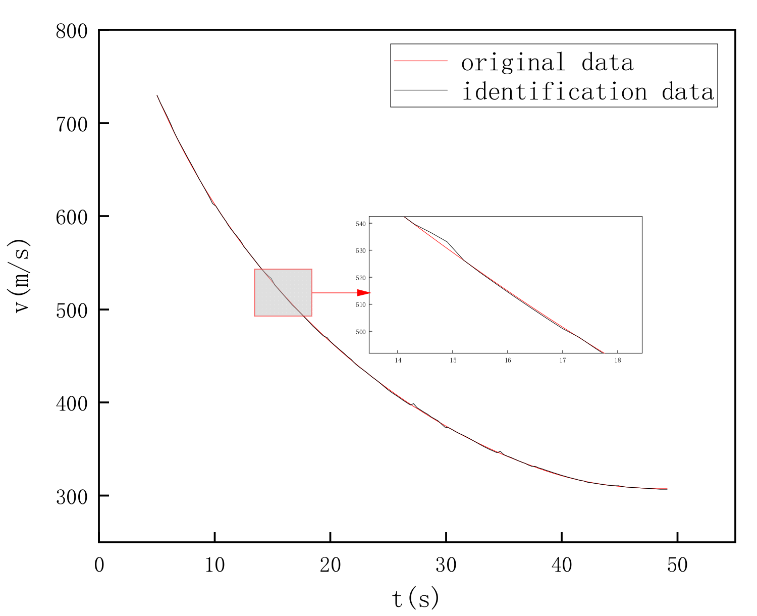This is used as the final result of the whole optimization process to achieve the optimal segmented quadratic polynomial fitting for these 54 radar data points, as shown in Figure 1, which shows the fitting result for the velocity $v$. The calculation formula of the fitness function is as follows:

$$fitness={\displaystyle \sum _{i=1}^{BP}(y_1(x_i)}-y_{mea}(x_i){)}^2+{\displaystyle \sum _{BP+1}^{N_{mea}}(y_2(x_i)}-y_{mea}(x_i){)}^2$$

(38)

where BP refers to segmented points; $N_{mea}$ refers to the number of points fitted each time, which is equal to 54; and $y_{mea}$ refers to the radar measurement data. Figure 1, respectively, shows the quadratic polynomial fitting of the data of 54 points using the improved Crayfish Optimization Algorithm (COA) and the Particle Swarm Optimization Algorithm (PSO). The results indicate that the fitting results of both algorithms are quite good. However, as a newly proposed algorithm, the COA algorithm takes into account some new problems and requirements in modern data processing in its design. In contrast, although the PSO algorithm is a classic and effective optimization algorithm when dealing with new types of real-time data, the COA algorithm can adapt to the changes in the data more naturally by utilizing its new features, demonstrating better flexibility and adaptability, especially in data-fitting scenarios such as projectile flight that have complex environments and real-time requirements.

3.3. Calculation of Roll Angular Velocity

In aerospace, navigation, and attitude control, it is of vital importance to accurately obtain the roll angular velocity of an object. As a key parameter describing the dynamic change of an object’s attitude, roll angular velocity is of great importance for the stable flight of aircraft and the precise motion control of robots. With the development of sensor technology, geomagnetic sensors have become an important means to obtain attitude information under their unique advantages. Through the geomagnetic data $m_x$, $m_y$, and $m_z$ measured by the three-axis geomagnetic sensor on board, the roll angular velocity of the projectile in the air can be calculated. Because the geomagnetic data $m_z$ corresponds to the rolling direction of the projectile, this paper only calculates the rolling angular velocity of the projectile based on the geomagnetic data $m_z$, and the specific calculation steps are shown below:

(1)

Determine the maximum and minimum values of the geomagnetic data $m_z$ and their corresponding times. Because the geomagnetic data have a sinusoidal shape, the maximum and minimum values of the geomagnetic data are determined for each cycle.

(2)

Calculate the average of the geomagnetic data over each cycle.

(3)

Find the crossing point. Traverse the geomagnetic data $m_z$ , and calculate the time at which all the geomagnetic data cross the median by interpolation.

(4)

Calculate the rotational speed: For the neighboring traversal points, calculate the time difference ($dtime$). Then, the formula for calculating the rotational speed $roll$ is:

$$roll=1/dtime$$

(39)

(5)

Calculate the roll angular velocity ${\omega }_{xi}$ .

$${\omega }_{xi}=2\pi \times roll$$

(40)

Figure 2 presents the detailed flow of processing the geomagnetic data. In the figure, the yellow, red, and green data respectively represent the maximum, minimum, and average values of the geomagnetic data within each period. First of all, it is necessary to find out the maximum and minimum values in each cycle from the geomagnetic data. After obtaining the maximum and minimum values, the average value is calculated, which is important in the whole process of geomagnetic data processing. Figure 3 shows the process of finding the crossing points of the geomagnetic data and calculating the angular velocity of the projectile roll. After determining these crossing points, the rolling angular velocity of the projectile is calculated according to Equations (39) and (40).

3.4. Parametric Differential Method (C-K Method)

The C-K method is a method proposed by Chapman and Kirk in 1969. This method involves the derivation of the variables of the system of equations for the parameters to be identified, forming a system of conjugate equations consisting of these derivatives and solving them together with the original equations. In prediction-related issues, the traditional ballistic extrapolation method has certain limitations. The aerodynamic parameters it uses are often obtained based on specific conditions or assumptions. When applied to the current environment, due to the complexity and variability of the environment, these aerodynamic parameters may deviate significantly from the actual situation. This deviation accumulates continuously during the ballistic extrapolation process, severely affecting the accuracy of the prediction results.

However, the C-K method provides us with a better solution. The C-K method identifies aerodynamic parameters based on current flight data. Current flight data contain abundant real-time information and can truly reflect the flight state in the current environment. Through effective processing and analysis of these data, the C-K method can accurately identify the real aerodynamic parameters that are in line with the current environment. Applying these real aerodynamic parameters to the prediction process can significantly reduce the errors caused by parameter deviation, thereby making the prediction results more accurate and reliable.

3.4.1. Introduction to the Principle

First, it is assumed that there is a system of equations containing $N_2$ first-order differential equations and a set of starting conditions, as shown in Equations (41) and (42) as follows:

$${\displaystyle \frac{{\mathrm{dy}}_m}{\mathrm{d}x}}=f(x,y_1,y_2,\cdot \cdot \cdot ,y_{N_2},{\mu }_1,{\mu }_2,\cdot \cdot \cdot ,{\mu }_{N_3},)$$

(41)

$${\mathrm{y}}_m{|}_{x=x_0}{=\mathrm{y}}_{m_0},m=1,2,\cdot \cdot \cdot ,N_2$$

(42)

where $x$ is the independent variable; $y_1,y_2,\cdot \cdot \cdot ,y_{N_2}$ are independent variables; $N_2$ is the number of independent variables and corresponding starting conditions;${\mu }_1,{\mu }_2,\cdot \cdot \cdot ,{\mu }_{N_3}$ are parameters to be determined; there are $N_3$ in total; and $y_{10},y_{20},\cdot \cdot \cdot ,y_{N_{20}}$ are the starting conditions.

Suppose that $N_1$($N_1\le N_2$) of the independent variables is measured at the i-th $(i=1,2,\cdot \cdot \cdot ,N_0)$ observation point’s value $y_{mea}$. The corresponding calculated value at the observation point is recorded as $y_m(x_i)$, and the following residual ($\epsilon$) is the objective function.

$$\epsilon ={\displaystyle \sum _{i=1}^{N_0}{\displaystyle \sum _{m=1}^{N_1}(y_{mea}-}}{y}_m(x_i))$$

(43)

To minimize the residuals, a set of parameters ${\mu }_1,{\mu }_2,\cdot \cdot \cdot ,{\mu }_{N_3}$ to be determined is chosen to make the $N_{23}$ partial derivatives of $\epsilon$ with respect to ${\mu }_k$ equal to 0, ${\displaystyle \frac{\partial \epsilon }{\partial {\mu }_k}}=0$, $N_{23}=N_3+N_2$. Therefore, $y_m(x_i)$ is expanded in the neighborhood of a given set of parameters, ${\mu }_j^{(0)}$, as shown in Equation (44):

$$y_m=y_m^{(0)}+{\displaystyle \sum _{j=1}^{N_{23}}\frac{\partial y_m}{\partial {\mu }_j}}△{\mu }_j$$

(44)

Substituting Equation (42) into Equation (41), $\epsilon$ is a function of $△{\mu }_j$, taking the partial derivatives of $\epsilon$ for each $△{\mu }_j$ and making the derivatives zero, the regular equation is obtained as follows:

$$A_1\cdot △\mu =B$$

(45)

where $A_1$ is a $N_{23}\times N_{23}$ matrix, $△\mu$ is a $N_{23}\times 1$ matrix, $B$ is a $N_{23}\times 1$ matrix.

The elements in $A_1$ are:

$$a_{lk}={\displaystyle \sum _{i=1}^{N_0}{\displaystyle \sum _{m=1}^{N_2}{p}_{ml}}}\cdot p_{mk}$$

(46)

where $l,k=1,2,\cdot \cdot \cdot ,N_{23}$.

The elements in $B$ are as follows:

$$b_k={\displaystyle \sum _{i=1}^{N_0}{\displaystyle \sum _{m=1}^{N_2}(y_{mea}-y_m^{(0)}(x_i))}}{p}_{mk}$$

(47)

The expression of $△{\mu }_j$ is shown in Equation (48):

$$△\mu ={(△{\mu }_1,△{\mu }_2,\cdot \cdot \cdot ,△{\mu }_{N_{23}})}^T$$

(48)

$$p_{mj}={\displaystyle \frac{\partial y_m}{\partial {\mu }_j}}$$

(49)

where $j=1,2,\cdot \cdot \cdot ,N_{23}$, the expression for the sensitivity coefficient $p_{mj}$ can be obtained by deriving the differential equation.

Given a set of parameters ${\mu }_j^{(0)}$, a new estimate of the parameter ${\mu }_j$ can be obtained by solving $△{\mu }_j$.

$${\mu }_j^{(1)}={\mu }_j^{(0)}+△{\mu }_j$$

(50)

Subsequently, ${\mu }_j^{(1)}$ is used to calculate $y_m(x_i)$ and $\epsilon$, which $\epsilon$ meets the accuracy requirement, the iterative calculation stops, and the last obtained ${\mu }_j^{(1)}$ is the final parameter value. Otherwise, ${\mu }_j^{(1)}$ is treated as ${\mu }_j^{(0)}$, and the iterative computation continues to modify ${\mu }_j$ until $\epsilon$ meets the accuracy requirements.

3.4.2. Derivation of Projectile Sensitivity Coefficients

The core purpose of this paper is to make real-time predictions of the landing point of a certain type of grenade during uncontrolled flight in the air. Among the many aerodynamic parameters affecting landing point prediction, the drag coefficient is the most critical factor, so only the drag coefficient can be recognized. To determine the drag coefficient $c_{x0}$, the sensitivity coefficients of the ballistic elements to the drag coefficient $c_{x_0}$, $v$, ${\theta }_a$, ${\psi }_2$, $x$, $y$, $z$, and ${\omega }_{xi}$ are defined as:

$$\begin{array}{l}{P}_{11}={\displaystyle \frac{\partial v}{\partial c_{x_0}}},P_{12}={\displaystyle \frac{\partial v}{\partial v}},P_{13}={\displaystyle \frac{\partial v}{\partial {\theta }_a}},P_{14}={\displaystyle \frac{\partial v}{\partial {\psi }_2}},P_{15}={\displaystyle \frac{\partial v}{\partial x}},P_{16}={\displaystyle \frac{\partial v}{\partial y}},P_{17}={\displaystyle \frac{\partial v}{\partial z}},P_{17}={\displaystyle \frac{\partial v}{\partial {\omega }_{xi}}}\\ P_{21}={\displaystyle \frac{\partial {\theta }_a}{\partial c_{x_0}}},P_{22}={\displaystyle \frac{\partial {\theta }_a}{\partial v}},P_{23}={\displaystyle \frac{\partial {\theta }_a}{\partial {\theta }_a}},P_{24}={\displaystyle \frac{\partial {\theta }_a}{\partial {\psi }_2}},P_{25}={\displaystyle \frac{\partial {\theta }_a}{\partial x}},P_{26}={\displaystyle \frac{\partial {\theta }_a}{\partial y}},P_{27}={\displaystyle \frac{\partial {\theta }_a}{\partial z}},P_{28}={\displaystyle \frac{\partial {\theta }_a}{\partial {\omega }_{xi}}}\\ P_{31}={\displaystyle \frac{\partial {\psi }_2}{\partial c_{x_0}}},P_{32}={\displaystyle \frac{\partial {\psi }_2}{\partial v}},P_{33}={\displaystyle \frac{\partial {\psi }_2}{\partial {\theta }_a}},P_{34}={\displaystyle \frac{\partial {\psi }_2}{\partial {\psi }_2}},P_{35}={\displaystyle \frac{\partial {\psi }_2}{\partial x}},P_{36}={\displaystyle \frac{\partial {\psi }_2}{\partial y}},P_{37}={\displaystyle \frac{\partial {\psi }_2}{\partial z}},P_{38}={\displaystyle \frac{\partial {\psi }_2}{\partial {\omega }_{xi}}}\\ P_{41}={\displaystyle \frac{\partial x}{\partial c_{x_0}}},P_{42}={\displaystyle \frac{\partial x}{\partial v}},P_{43}={\displaystyle \frac{\partial x}{\partial {\theta }_a}},P_{44}={\displaystyle \frac{\partial x}{\partial {\psi }_2}},P_{45}={\displaystyle \frac{\partial x}{\partial x}},P_{46}={\displaystyle \frac{\partial x}{\partial y}},P_{47}={\displaystyle \frac{\partial x}{\partial z}},P_{48}={\displaystyle \frac{\partial x}{\partial {\omega }_{xi}}}\\ P_{51}={\displaystyle \frac{\partial y}{\partial c_{x_0}}},P_{52}={\displaystyle \frac{\partial y}{\partial v}},P_{53}={\displaystyle \frac{\partial y}{\partial {\theta }_a}},P_{54}={\displaystyle \frac{\partial y}{\partial {\psi }_2}},P_{55}={\displaystyle \frac{\partial y}{\partial x}},P_{56}={\displaystyle \frac{\partial y}{\partial y}},P_{57}={\displaystyle \frac{\partial y}{\partial z}},P_{57}={\displaystyle \frac{\partial y}{\partial {\omega }_{xi}}}\\ P_{61}={\displaystyle \frac{\partial z}{\partial c_{x_0}}},P_{62}={\displaystyle \frac{\partial z}{\partial v}},P_{63}={\displaystyle \frac{\partial z}{\partial {\theta }_a}},P_{64}={\displaystyle \frac{\partial z}{\partial {\psi }_2}},P_{65}={\displaystyle \frac{\partial z}{\partial x}},P_{66}={\displaystyle \frac{\partial z}{\partial y}},P_{67}={\displaystyle \frac{\partial z}{\partial z}},P_{67}={\displaystyle \frac{\partial z}{\partial {\omega }_{xi}}}\\ P_{71}={\displaystyle \frac{\partial {\omega }_{xi}}{\partial c_{x_0}}},P_{62}={\displaystyle \frac{\partial {\omega }_{xi}}{\partial v}},P_{63}={\displaystyle \frac{\partial {\omega }_{xi}}{\partial {\theta }_a}},P_{64}={\displaystyle \frac{\partial {\omega }_{xi}}{\partial {\psi }_2}},P_{65}={\displaystyle \frac{\partial {\omega }_{xi}}{\partial x}},P_{66}={\displaystyle \frac{\partial {\omega }_{xi}}{\partial y}},P_{67}={\displaystyle \frac{\partial {\omega }_{xi}}{\partial z}},P_{67}={\displaystyle \frac{\partial {\omega }_{xi}}{\partial {\omega }_{xi}}}\end{array}$$

where the initial value of each sensitivity coefficient is as follows:

$${\displaystyle \frac{\partial y_m}{\partial {\mu }_j}}=p_{mj}(x_0)\left\{\begin{array}{l}=1,y_m={\mu }_j\\ =0, other\end{array}\right.$$

(51)

The following is an example of the derivation of the sensitivity coefficients of the ballistic parameter $v$ for $c_{x_0}$, $v$, ${\theta }_a$, ${\psi }_2$, $x$, $y$, $z$, and ${\omega }_{xi}$, respectively:

$$\begin{array}{l}{\displaystyle \frac{\mathrm{d}{P}_{11}}{\mathrm{d}t}}={\displaystyle \frac{\partial }{\partial c_{x_0}}}({\displaystyle \frac{\mathrm{d}v}{\mathrm{d}t}})=-{\rho }^{\text{'}}{\displaystyle \frac{v^{2}S{c}_{x_0}}{2m}}{P}_{51}-{\displaystyle \frac{\rho vS}{m}}{c}_{x_0}{P}_{11}\\ -{\displaystyle \frac{\rho v^{2}S}{2m}}-g\cos {\theta }_a\cos {\psi }_2{P}_{21}+g\sin {\theta }_a\sin {\psi }_2{P}_{31}\end{array}$$

(52)

$$\begin{array}{l}{\displaystyle \frac{\mathrm{d}{P}_{12}}{\mathrm{d}t}}={\displaystyle \frac{\partial }{\partial v}}({\displaystyle \frac{\mathrm{d}v}{\mathrm{d}t}})=-{\rho }^{\text{'}}{\displaystyle \frac{v^{2}S{c}_{x_0}}{2m}}{P}_{52}-{\displaystyle \frac{\rho vS}{m}}{c}_{x_0}{P}_{12}\\ -g\cos {\theta }_a\cos {\psi }_2{P}_{22}+g\sin {\theta }_a\sin {\psi }_2{P}_{32}\end{array}$$

(53)

$$\begin{array}{l}{\displaystyle \frac{\mathrm{d}{P}_{13}}{\mathrm{d}t}}={\displaystyle \frac{\partial }{\partial {\theta }_a}}({\displaystyle \frac{\mathrm{d}v}{\mathrm{d}t}})=-{\rho }^{\text{'}}{\displaystyle \frac{v^{2}S{c}_{x_0}}{2m}}{P}_{53}-{\displaystyle \frac{\rho vS}{m}}{c}_{x_0}{P}_{13}\\ -g\cos {\theta }_a\cos {\psi }_2{P}_{23}+g\sin {\theta }_a\sin {\psi }_2{P}_{33}\end{array}$$

(54)

$$\begin{array}{l}{\displaystyle \frac{\mathrm{d}{P}_{14}}{\mathrm{d}t}}={\displaystyle \frac{\partial }{\partial {\psi }_2}}({\displaystyle \frac{\mathrm{d}v}{\mathrm{d}t}})=-{\rho }^{\text{'}}{\displaystyle \frac{v^{2}S{c}_{x_0}}{2m}}{P}_{54}-{\displaystyle \frac{\rho vS}{m}}{c}_{x_0}{P}_{14}\\ -g\cos {\theta }_a\cos {\psi }_2{P}_{24}+g\sin {\theta }_a\sin {\psi }_2{P}_{34}\end{array}$$

(55)

$$\begin{array}{l}{\displaystyle \frac{\mathrm{d}{P}_{15}}{\mathrm{d}t}}={\displaystyle \frac{\partial }{\partial x}}({\displaystyle \frac{\mathrm{d}v}{\mathrm{d}t}})=-{\rho }^{\text{'}}{\displaystyle \frac{v^{2}S{c}_{x_0}}{2m}}{P}_{55}-{\displaystyle \frac{\rho vS}{m}}{c}_{x_0}{P}_{15}\\ -g\cos {\theta }_a\cos {\psi }_2{P}_{25}+g\sin {\theta }_a\sin {\psi }_2{P}_{35}\end{array}$$

(56)

$$\begin{array}{l}{\displaystyle \frac{\mathrm{d}{P}_{16}}{\mathrm{d}t}}={\displaystyle \frac{\partial }{\partial y}}({\displaystyle \frac{\mathrm{d}v}{\mathrm{d}t}})=-{\rho }^{\text{'}}{\displaystyle \frac{v^{2}S{c}_{x_0}}{2m}}{P}_{56}-{\displaystyle \frac{\rho vS}{m}}{c}_{x_0}{P}_{16}\\ -g\cos {\theta }_a\cos {\psi }_2{P}_{26}+g\sin {\theta }_a\sin {\psi }_2{P}_{36}\end{array}$$

(57)

$$\begin{array}{l}{\displaystyle \frac{\mathrm{d}{P}_{17}}{\mathrm{d}t}}={\displaystyle \frac{\partial }{\partial z}}({\displaystyle \frac{\mathrm{d}v}{\mathrm{d}t}})=-{\rho }^{\text{'}}{\displaystyle \frac{v^{2}S{c}_{x_0}}{2m}}{P}_{57}-{\displaystyle \frac{\rho vS}{m}}{c}_{x_0}{P}_{17}\\ -g\cos {\theta }_a\cos {\psi }_2{P}_{27}+g\sin {\theta }_a\sin {\psi }_2{P}_{37}\end{array}$$

(58)

$$\begin{array}{l}{\displaystyle \frac{\mathrm{d}{P}_{18}}{\mathrm{d}t}}={\displaystyle \frac{\partial }{\partial {\omega }_{xi}}}({\displaystyle \frac{\mathrm{d}v}{\mathrm{d}t}})=-{\rho }^{\text{'}}{\displaystyle \frac{v^{2}S{c}_{x_0}}{2m}}{P}_{58}-{\displaystyle \frac{\rho vS}{m}}{c}_{x_0}{P}_{18}\\ -g\cos {\theta }_a\cos {\psi }_2{P}_{28}+g\sin {\theta }_a\sin {\psi }_2{P}_{38}\end{array}$$

(59)

The derivation of the sensitivity coefficients of the other ballistic parameters ${\theta }_a$, ${\psi }_2$, $x$, $y$, $z$, and ${\omega }_{xi}$ for $c_{x_0}$, $v$, ${\theta }_a$, ${\psi }_2$, $x$, $y$, $z$, and ${\omega }_{xi}$, respectively, are similar to the above process. To maintain the length and clarity of this paper, these derivations are not repeated here.

3.5. Real-Time Impact Point Prediction Methods

In modern military and related fields, the prediction of the projectile’s point of impact during flight has always been a subject of great concern and a very challenging one. When a projectile is in flight, it is affected by a variety of complex factors, such as aerodynamic forces, meteorological conditions, and its physical properties, which are intertwined with each other, making it difficult to accurately predict the projectile’s landing point in a clear and timely manner. Because of this, to effectively solve the key problem of difficulty in accurately and timely predicting the projectile landing point during the flight process, this paper proposes an improved ballistic real-time landing point prediction method.

In this paper, the fitting operation is carried out for the radar measurement data and the geomagnetic data. When the projectile passes the apex of the trajectory (i.e., the velocity is minimized), the C-K method in Section 3.4 is applied to identify the drag coefficient of the projectile based on all the radar measurements, as well as the roll angular velocity data calculated from the geomagnetic data. Once the radar has obtained 54 sets of data before the projectile reaches the apex of the trajectory, a segmented quadratic polynomial fit is implemented using the improved crayfish optimization algorithm in Section 3.1.4. The radar measurement data of the 28th point after fitting is selected, and according to the time $t_0$ corresponding to the 28th point, the geomagnetic data acquired by the geomagnetic sensor during ($t_0-0.5$, $t_0+0.5$) is selected to calculate the roll angular velocity, and the improved crayfish optimization algorithm is applied again to fit the calculated roll angular velocity. After that, the radar measurement data and roll angular velocity corresponding to time $t_0$ are selected and substituted into the projectile motion model in Section 1 to carry out the landing point prediction, and the fitting prediction is carried out continuously in this way (such as data of points 1–54, 2–55). After the projectile passes the apex of the trajectory, the drag coefficients identified by the C-K method are applied to the projectile motion model in Section 1, and the same fitting method and projectile motion model are subsequently used to perform the impact point prediction.

The flowchart of fallout prediction is shown in Figure 4:

4. Simulation Experiment and Verification

To verify the correctness and accuracy of the method proposed in this paper, the actual flight data of a high-speed rotating tail projectile is taken as an example. The flight data of the projectile includes radar measurement data $v_x$, $v_y$, $v_z$, $x$, $y$, $z$, and geomagnetic data $m_x$, $m_y$, $m_z$ measured by a three-axis geomagnetic sensor. Under the same test data conditions, the traditional four-degree-of-freedom model fallout prediction method and the method proposed in this paper based on the improved crayfish optimization algorithm for trajectory fitting and combined with the parameter identification of the C-K method for fallout prediction are compared.

The meteorological conditions shown in Figure 5 and Figure 6 were used. Specifically, Figure 5 meticulously presents the distribution of wind speed at different altitudes. The numerical magnitude of these wind speed data and its change rule with height have an inestimable impact on the aerodynamic characteristics during the flight of the projectile. It can be clearly seen from Figure 5 that in the high-altitude area with an altitude ranging from 8000 to 10,000 m, the wind speed shows a relatively large trend. Figure 6 further supplements the information related to wind direction. The specific direction of the wind, as well as the size of the wind speed, the directional properties of both, and their change patterns over time, have a great impact on the trajectory of the projectile flight, speed, and the final landing point. These meteorological conditions are important components of the overall projectile flight environment and provide a unified external environment setting for subsequent comparison of different impact point prediction methods based on the same test data. In the low-altitude data shown in Figure 6, a sudden fluctuation phenomenon can be observed. This phenomenon is mainly attributed to the display mechanism of the shooting direction angle. In this study, the measurement of the shooting direction angle uses a circumferential measurement range of 360 degrees. When the shooting direction angle exceeds 360 degrees during the flight of the projectile, to adapt to the data display and recording system, its value are converted to a relatively smaller degree for display. For example, if the actual shooting direction angle reaches 370 degrees, it will be displayed as 10 degrees in the data recording and chart presentation.

After the projectile crosses the apex of the trajectory (this point is the lowest point of velocity), the aerodynamic parameter identification is carried out by utilizing the method of calculating the rolling angular velocity of the projectile described in Section 3.3 and Section 3.4, as well as the C-K method to identify all the data measured by the radar and the rolling angular velocity. In the process of aerodynamic parameter identification using the C-K method, the ballistic trajectory is divided into multiple intervals using the interval constant method, and the time step of the ballistic data in each interval is set to 0.05 s, and the aerodynamic physical parameter values in each interval are assumed to be fixed, to identify the aerodynamic parameters in each interval.

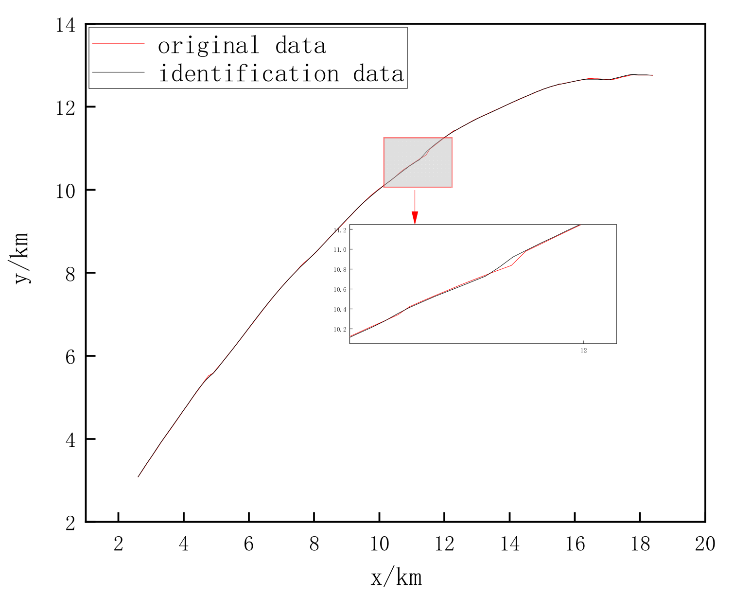
Since the time interval of the radar-measured data is not fixed and is basically around 100 ms, and the parameter identification by the C-K method is based on the physical model of the projectile, it is necessary to carry out a linear interpolation process on the measured data, interpolating them into the data with a fixed time interval of 0.05 s. Then, the aerodynamic parameter identification work is carried out for these interpolated data, and the identification results are shown in Figure 7, Figure 8 and Figure 9. From Figure 7 and Figure 8, it can be found that the deviation between the result $v$, $x$, and $y$ identified by the C-K method and the original data after ballistic fitting is small, thus verifying the accuracy of the C-K method. Subsequently, the correspondence between the drag coefficient $c_{x_0}$ and Mach number $Ma$ in Figure 9 is substituted into the projectile motion model in Section 2.

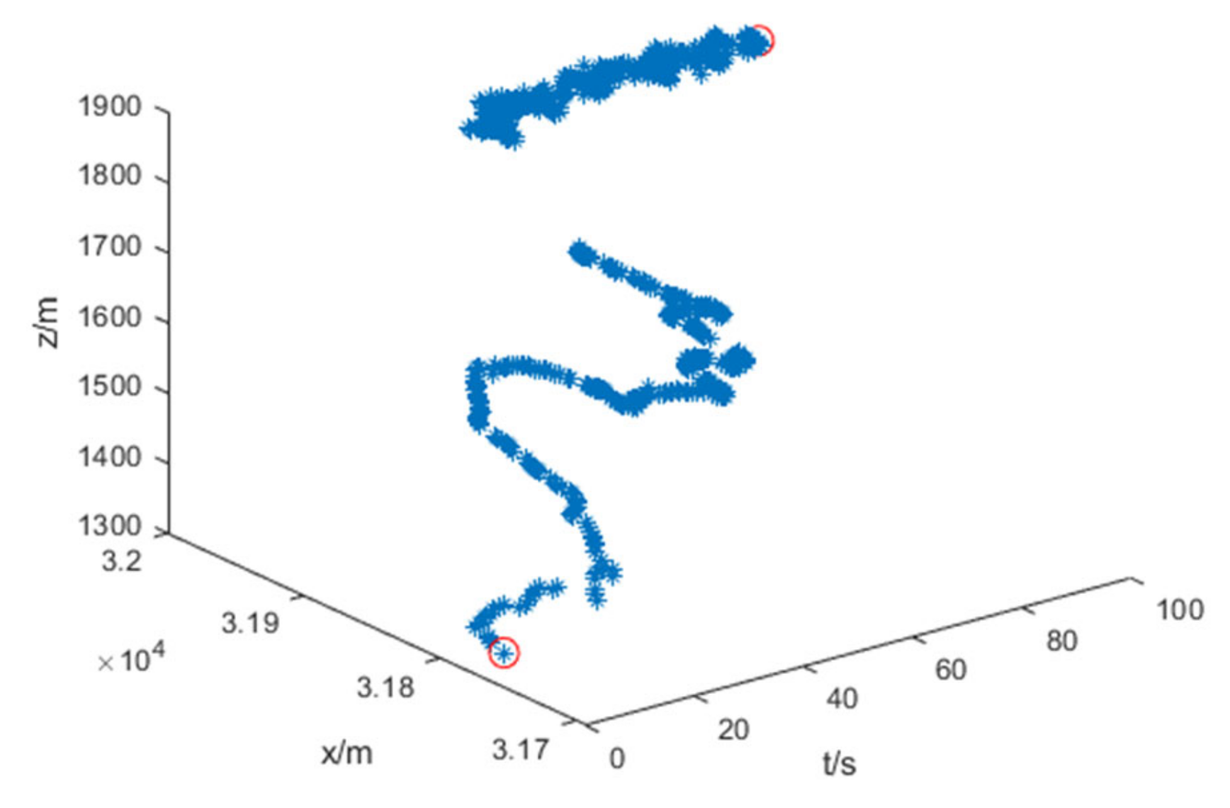
Following the method described in Figure 4 in Section 3.5, real-time fallout prediction is carried out for the real flight data of the high-speed rotating tail projectile, and the fallout prediction results are shown in Figure 10. It can be seen that after the projectile passes through the top of the trajectory, the aerodynamic parameters identified by the C-K method are substituted into the four-degree-of-freedom model for the fall point prediction, and the predicted results are closer to the final fall point (31,970.6 m, 1826.3 m) than the results without identifying the aerodynamic parameters by the C-K method. 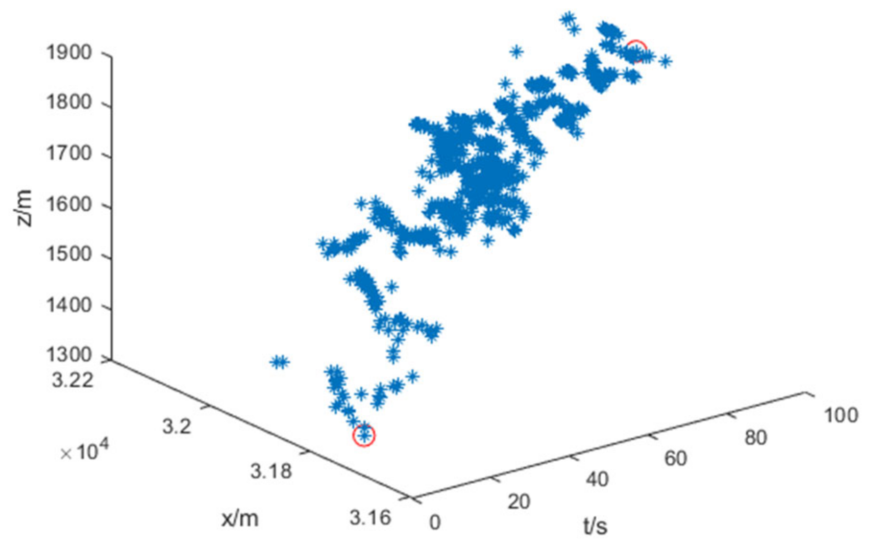Figure 11 illustrates the results of the fallout point prediction using the conventional four-degree-of-freedom model. It can be found that there is a large deviation between the identified results and the final impact point because no fitting operation was performed on the radar measurement data and the C-K method was not applied to identify the aerodynamic parameters. Among them, the red circles in Figure 10 and Figure 11 represent the initial point and the final point of the predicted landing point of the projectile, while the blue circles represent the predicted landing points at other moments.

In Figure 12 and Figure 13, “curve 1” represents the case of impact point prediction using the method proposed in this paper, and “curve 2” represents the case of impact point prediction using the traditional four-degree-of-freedom model. From Figure 12 and Figure 13, the simulation results demonstrate that, compared with the traditional model, the method proposed in this paper shows significant advantages in the prediction of projectile impact points. Specifically, through the processing and analysis of the actual flight data of a high-speed rotating fin-stabilized projectile, it can be known that the deviation between the impact points predicted by the new method and the actual results has been minimized. This accuracy stems from the meticulous design of each part of the method. In this method, the improved crayfish optimization algorithm can fit the curve according to the changing trend of the data, making the fitting result closer to the real-flight trajectory of the projectile. Meanwhile, the C-K method also plays a crucial role in the entire prediction process. The C-K method can accurately identify the aerodynamic parameters based on the actual flight data within each small interval. Moreover, considering that the time interval of the radar measurement data is not fixed (about 100 ms), the linear interpolation processing is carried out to make the data interval 0.05 s, further ensuring the accuracy of the C-K method. From the perspective of practical application, this method can be used in the engineering field to optimize the projectile design and testing process, improving the design efficiency and testing accuracy. In terms of trajectory analysis, it can provide researchers with more accurate information on the projectile’s flight path and impact point, helping to gain an in-depth understanding of the projectile’s flight characteristics. In the military environment, accurate prediction of impact points is of great significance for improving strike accuracy and reducing collateral damage. By reducing the prediction deviation, the new method can better meet the strict requirements of these practical application scenarios for the prediction of projectile impact points, thus showing excellent practical effectiveness. Therefore, this method has broad application prospects in engineering, trajectory analysis, military environment, and other fields.

The analysis of the data in Figure 12 and Figure 13 reveals that within 100 s, the range coverage and lateral deviation of the projectile are relatively large. This research aims to predict the entire flight trajectory and the landing point of the projectile. The accuracy of the landing point prediction varies with the flight stage. During the first half of the projectile’s flight, due to the combined influence of various factors, there is a significant deviation between the predicted landing point and the actual landing point, which is in line with the laws of physics and the actual situation. When the projectile exits the muzzle, its initial state has a high degree of uncertainty. Although factors such as the launching angle, initial velocity, and initial disturbance at the muzzle have been calibrated to some extent before launching, it is still difficult to achieve absolute precision. Minor deviations are rapidly amplified as the flight progresses. For example, even a slight deviation in the launching angle causes the flight trajectory of the projectile to gradually deviate from the ideal path under the influence of external forces such as air resistance and gravity, resulting in a significant increase in the deviation of the landing point prediction. During this stage, within a specific 100 s, situations such as the projectile covering a flight range of 200 m and having a lateral deviation of 500 m may occur, which reflects the actual situation of the large deviation in the landing point prediction during the first half of the flight. During the second half of the projectile’s flight, the accuracy of the landing point prediction gradually improves. Firstly, the projectile is continuously corrected by the external environment during the flight. As the flight time increases, the adjusting effect of air resistance on the flight attitude of the projectile becomes more and more obvious, meaning the flight trajectory tends to be stable. Secondly, after obtaining more flight data, the prediction algorithm can optimize the prediction model based on the real-time data. By continuously monitoring information, such as the speed and position of the projectile, the prediction algorithm can consider various influencing factors more accurately, thereby continuously narrowing the gap between the predicted landing point and the actual landing point. Therefore, the later the landing point prediction is made, the more accurate the result will be, and the higher the degree of coincidence with the actual landing point will be.

In conclusion, the relevant data of the projectile’s flight within different time intervals in Figure 12 and Figure 13, including the data showing large deviations in the first half and the data tending to be accurate in the second half, accurately reflect the actual situation of the landing point prediction throughout the entire flight process of the projectile. They are in line with the laws of physics and are reasonable in the research context, providing an important basis for understanding the flight characteristics of the projectile and the evolution process of the landing point prediction.

5. Conclusions

In this study, a projectile-landing-point prediction method integrating the improved crayfish algorithm and the C-K method is proposed, aiming at solving the problem that it is difficult to predict the landing point of a projectile in flight in a clear and timely manner. Through a series of analysis and validation, the following conclusions are drawn:

• The improved crayfish optimization algorithm shows excellent performance in data segmentation fitting. From the fitting results, it can be seen that its fitting curve is largely consistent with the original data, which means that the algorithm can process the data efficiently and construct a solid data foundation for subsequent landing point prediction.
• Concerning the processing of geomagnetic data, this study can accurately obtain key information, such as the maximum value, the minimum value, and the crossing point, and accordingly calculate important parameters, such as the roll angular velocity, to provide multi-dimensional data support for the prediction of the projectile’s landing point.
• When recognizing the aerodynamic parameters after the projectile crosses the apex of the trajectory, because the time interval of the radar measurement data is not fixed, this research adopts the reasonable means of linear interpolation and other means of processing, and the recognition results obtained using the C-K method have a small deviation from the original data, which strongly proves that the C-K method has the accuracy and rapidity of aerodynamic parameter recognition.
• The results of this research provide an effective method for projectile design, ballistic analysis, and fallout prediction in practical engineering, which helps to improve the accuracy and reliability of related engineering applications. Although the current method has achieved good results, there is still room for improvement. For example, the crawfish algorithm can be further optimized to improve the computational efficiency or the applicability of the method in more complex meteorological conditions can be explored, which points out the direction for future research.