Effects of the Uncertainty of Wall Distance on the Simulation of Turbulence/Transition Phenomena

Abstract

The uncertainty of the turbulence/transition model is a problem with relatively high attention in the CFD area. Wall distance is an important physical parameter in turbulence/transition modeling, and its accuracy has a large effect on numerical simulation results. As most CFD solvers use the solving strategy to calculate the nearest distance to the wall based on mesh topology, this makes wall distance one important source of the uncertainty of the simulation results. To investigate the role of wall distance in turbulence/transition simulations, we have conducted simulations for various aerodynamic shapes, such as the plate with zero pressure gradient (ZPG), RAE2822 supercritical airfoil and ONERA M6 transonic wing. Further, the prediction abilities on turbulence/transition and shock wave phenomena of several physical models, including SA, SST and Wilcox-k-ω turbulence models as well as the γ-Re_θt-SST transition model, are analyzed with different degrees of mesh orthogonality. The results imply that the numerical solution of wall distance in the boundary layer has a relatively large error when the mesh orthogonality is bad, having a large effect on the accuracy of the turbulence/transition model. In detail, the Wilcox-k-ω turbulence model is unaffected by mesh orthogonality; under the condition of mesh non-orthogonality, the SA model leads to a substantially larger friction drag and change in the location of shock wave; the SST model also leads to a larger friction drag under the condition of mesh non-orthogonality, whose effect is much less than that for SA model; and the γ-Re_θt-SST model leads to a substantial upstream shift of transition location.

1. Introduction

With the rapid development and decreased cost of computer techniques, the numerical simulation technique based on CFD (Computational Fluid Dynamics) is widely used in engineering applications and teaching areas. Currently, it is commonly realized that the practical CFD technique is still the solving method based on the RANS (Reynolds Averaged Navier–Stokes) equation [1,2,3]. The advanced methods for turbulence simulation, such as LES (Large Eddy Simulation) [4,5,6] and DES (Detached Eddy Simulation) [7,8,9], are basically limited to simple geometry configurations with the magnitude of Reynolds number less than O (10⁷). In RANS methodology, the EVM (Eddy Viscosity Model) has the advantages of good robustness, simple operation and low cost, and has been widely used in the simulation of wall turbulence in aerospace engineering. The EVM includes the turbulence model and transition model. Improving the EVM still has important scientific value and application value, with the uncertainty of the turbulence model needing to be investigated further [10,11,12,13,14].

The wall distance d, an important physical quantity in EVM modeling, is used to model the wall behavior of turbulent flows. In the Prandtl mixing-length theory, the mixing length is set to be proportional to wall distance d with the Karman constant as the proportional coefficient:

$$l=\kappa d$$

(1)

In aerospace engineering, the turbulence models with high recognition are those based on the transportation equation, with wall distance used directly. For example, in the SA model developed by Spalart and Allmara [15], the dissipation term and generation term both use wall distance directly. In the k-ω SST model developed by Menter [16], the layering mixing function F₁ distinguishing the k-ω model in the inner layer from the k-ε model in the outer layer and the mixing function F₂ in the transportation region of shear stress both use wall distance. In the γ-Re_θt-SST model [17] developed by Langtry and Menter, the vorticity Reynolds number used for judging transition triggering uses the square of wall distance. Except the above ones, some models do not use wall distance, such as the k-ω model proposed by Wilcox [18] and its subsequent versions.

The computation method of wall distance can be classified into two classes: the method of solving the PDE (Partial Differential Equation) [19,20] and the direct computation method [21,22,23,24] based on searching and comparison. The usage of the PDE method needs additional computation cost and the computation accuracy of wall distance is easily affected by numerical discretization accuracy, poorly adapted for complex geometries. In practical applications, the direct computation method is more frequently chosen. Depending on the method of data structure storage for preconditioning, the direct computation method can be divided into several categories such as the enumeration method, layer-by-layer fast algorithm [21], loop box method [22], and ADT algorithm (alternative digital tree) [23,24].

The accuracy of wall distance derived by the direct computation method relies on the topology of original mesh. That is, it is critical whether the two mesh points closest to the object surface are in the corresponding normal line. The geometry shapes of complex aviation configurations have many curved surfaces. At the locations of the leading edge of the wing, the trailing edge of the wing and the combination surface of the wing and the fuselage, the mesh orthogonality is difficult to be ensured and the mesh quality in the boundary layer is not good, leading to the deviation of the mesh points near the wall from the normal line, as shown in Figure 1. As the wall distance derived by the direct computation method depends on the mesh topology structure near the wall greatly, the investigation of the effects of wall distance on the uncertainty of turbulence/transition simulation results has important application values for guiding mesh generation and estimating the correctness of the computational results.

In this paper, with the mesh topology derived in the way of ‘block to block’ as a research object, the near-wall flows at high Reynolds number, including those around a plate and a wing at transonic conditions, are systematically analyzed with common turbulence/transition models used. The wall distances with different accuracies were obtained by changing the mesh orthogonality, and the effects of the uncertainty of wall distance on turbulence/transition behaviors were realized.

2. Materials and Methods

2.1. Introduction of Turbulence Model

This paper uses the unified name strategy from NASA Turbulence Model Resources (TMR) [26]. The chosen turbulence/transition models were the “Standard” one-equation SA model [15], Menter SST model (SST-2003) [16], Wilcox-k-omega model (Wilcox1988) [18] and four-equation SST-LM transition model (γ-Re_θt-SST) [17]. In the following, the above models are represented by the SA model, SST model, Wilcox-k-ω model and γ-Re_θt-SST model, respectively.

The SA model is a common one, combining the empirical relationships of boundary layer turbulence in the algebraic zero-equation model. The critical empirical relationships are obtained based on the normal distributions of turbulent variables found in experiments, determining the basic features of the turbulence model. Thus, both the generation term and the dissipation term in the SA model use wall distance directly to modelize the near-wall distribution of transportation viscous coefficient ($\tilde{\nu }$). The following Formula (2) is one part of the generation term:

$$\tilde{S}=\Omega +{\displaystyle \frac{\tilde{\nu }}{{\kappa }^2{d}^2}}{f}_{v2}$$

(2)

where $\tilde{S}$ is the intermediate variable, $\Omega$ is the magnitude of vorticity, $\kappa$ is the Karmen constant, $\tilde{\nu }$ is the SA working variable and obeys the transport equation, d is wall distance, which is the distance from the field point to the nearest wall and $f_{\nu 2}$ is the near-wall harmonic function. The dissipation term D_dissipation also uses the wall distance directly:

$$D_{\mathrm{dissipation}}=\left[c_{w1}{f}_w-{\displaystyle \frac{c_{b1}}{{\kappa }^2}}{f}_{t2}\right]{\left({\displaystyle \frac{\tilde{\nu }}{d}}\right)}^2$$

(3)

where c_w1 and c_b1 are model closures and the function f_w uses wall distance d again to identify the logarithmic layer in turbulent boundary layer.

$$\begin{array}{l}{f}_w=g{\left({\displaystyle \frac{1+c_{w3}^6}{g^6+c_{w3}^6}}\right)}^{1/6}\\ g=r+c_{w2}(r^6-r)\\ r=\min \left({\displaystyle \frac{\tilde{\nu }}{\tilde{S}{\kappa }^2{d}^2}},10\right)\end{array}$$

(4)

The Menter SST model uses the wall distance in the layering mixing function F₁, which is utilized to distinguish the inner layer from the outer layer and has the following form:

$$\begin{array}{l}{F}_1=\tan \mathrm{h}\left({\arg }_1^4\right)\\ {\arg }_1=\min \left[\max \left({\displaystyle \frac{\sqrt{k}}{{\beta }^{*}\omega d}},{\displaystyle \frac{500\nu }{d^2\omega }}\right),{\displaystyle \frac{4\rho {\sigma }_{\omega 2}k}{{\mathrm{CD}}_{k\omega }{d}^2}}\right]\end{array}$$

(5)

where β^*, σ_ω2 are model closures, k is turbulent kinetic energy and ω is the dissipation rate of the transport equations of the SST model, d is wall distance and CD_kω is an intermediate function from the dimensional analysis. Another important mixing function F₂ in the SST model, which is used to identify the free shear layer and applies the empirical relationship between shear stress and turbulent kinetic energy, is shown in the following:

$$\begin{array}{l}{F}_2=\tan \mathrm{h}\left({\arg }_2^2\right)\\ {\arg }_2=\max \left(2{\displaystyle \frac{\sqrt{k}}{{\beta }^{*}\omega d}},{\displaystyle \frac{500\nu }{d^2\omega }}\right)\end{array}$$

(6)

The γ-Re_θt-SST model can realize automatic transition prediction by means of two transportation equations including empirical relationships, with the intermittent factor γ and the transition Reynolds number of momentum thickness Re_θt as transportation variables. The core parameter of this model is the vorticity Reynolds number Re_v, which is used to represent the unstable degree of flow direction. When Re_v exceeds the critical transition Reynolds number of momentum thickness, the transition process is triggered. The construction of this critical parameter uses the square of the wall distance:

$$R{e}_v={\displaystyle \frac{\rho d^{2}S}{\mu }}$$

(7)

where ρ is the density, S is strain-rate and μ is the coefficient of eddy viscosity.

2.2. Computational Code

The solver is the self-developed turbulence model developing platform (UTMDP) [27]. Based on the lattice method and unstructured mesh, this platform solves three-dimensional steady/unsteady RANS equations. For spatial discretization, the central scheme is used with the addition of artificial viscosity. For time marching, the LU-SGS implicit scheme is used. The platform contains the common turbulence/transition models. In the computation, the multigrid strategy is used to accelerate convergence, and the ‘block to block’ splitting strategy of structure mesh is used to generate regular hexahedral meshes. The wall distance is obtained by using the ADT (alternative digital tree) algorithm.

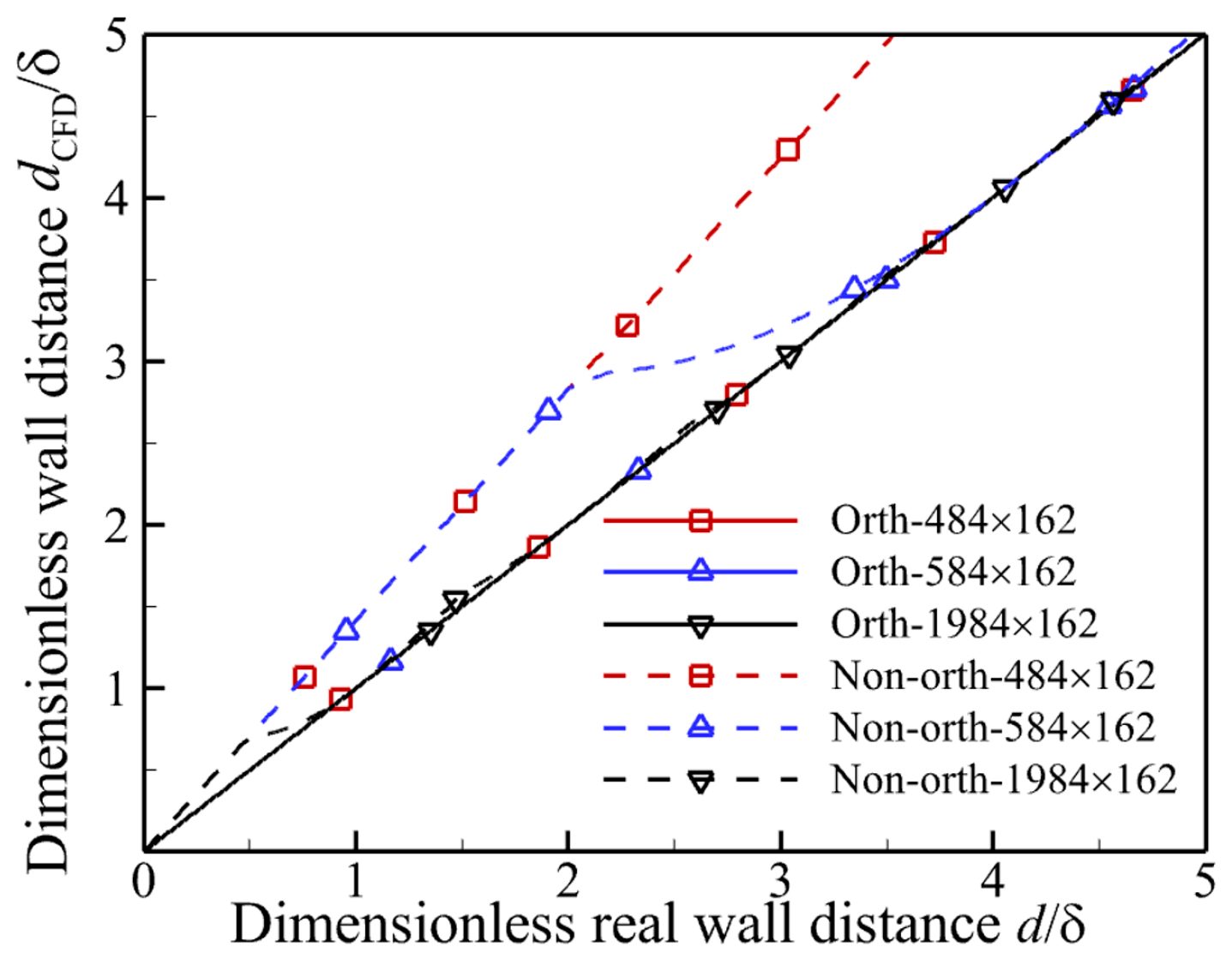
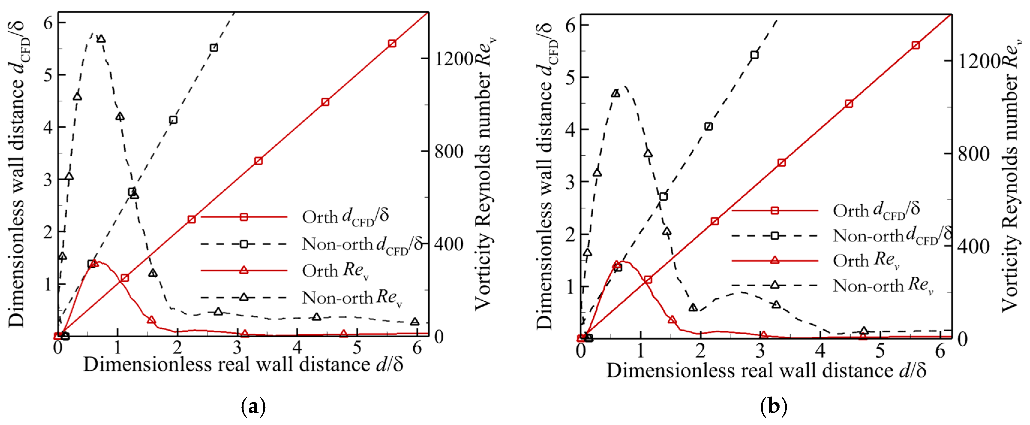
2.3. The Analysis of the Relationship Between Wall Distance and Mesh

When the mesh orthogonality near the wall is relatively bad, the distributions of spatial inner points may not be perpendicular to the wall and the wall distance derived is not the shortest one. Figure 2 shows the geometry relationship between the wall distance with the orthogonal mesh and that with the non-orthogonal mesh for the flat plate case. The side of the non-orthogonal mesh has an intersection angle θ with the normal direction of the object surface, the diameter of the circle O is the length of streamwise unit mesh Δx and point C is the intersection of the circle O and oblique mesh.

(1) When the actual wall distance d < Δx/2 (the length of OC), the computational value is represented by Formula (8) and |AC| = |CB|. For a non-orthogonal mesh, the spatial point lies in the inner part of the circle O (point D), and the wall distance from the direct computation method is the length of line segment AD. Actually, the wall distance should be the length of AE. The two line segments have the following relationship:

$$\mathrm{AD}\times \cos \theta =\mathrm{AE}$$

(8)

(2) When |OC| < d < |BG| = Δx/tanθ, the computational value is equal to the length of BF, larger than the actual wall distance |OC|. Until the spatial point lies at the locations perpendicular to the wall point (point G), the wall distance from the direct computation method is the actual one.

(3) When the actual wall distance d > |BG|, the derived wall distance with non-orthogonal mesh is the one at point B or the closest point at the right side of point B, which is still larger than the actual wall distance.

The variation of the derived wall distance with non-orthogonal mesh along the normal direction is shown in Figure 3. It can be seen that the uncertainty of wall distance originates from the oblique degree of mesh θ and the size of streamwise mesh Δx. When the streamwise mesh is refined, the radius of circle O is decreased, as shown in Figure 4.

3. Results

3.1. The Flat Plate with ZPG

The S-K flat plate [28] was chosen for the case of the flat plate with ZPG. Its transition in the boundary layer is a typical behavior of natural transition and is often used to investigate the simulation ability of the transition model for T-S transition [29]. We have applied the Wilcox-k-ω model, SA model, SST model and γ-Re_θt-SST model for the simulation of flat plate flow, with the purpose of investigating the simulation abilities of turbulence/transition models with orthogonal or non-orthogonal meshes.

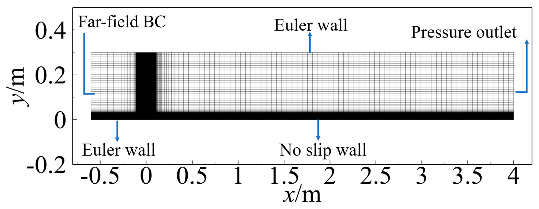
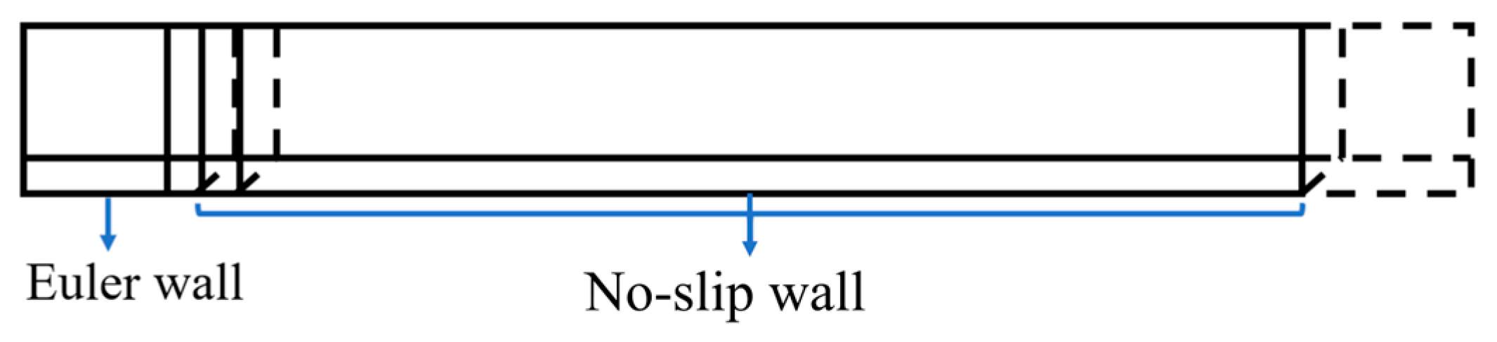
3.1.1. Mesh and Boundary Condition

The orthogonal and non-orthogonal structured meshes generated by the ‘block to block’ type were used. The geometry and the boundary conditions used are shown in Figure 5, where both the transition region from the Euler boundary to no-slip boundary at the leading edge and the normal direction are refined. The length of the flat plate was 4 m, the height of far-field was 0.3 m, the length of freestream region at the upstream side of the flat plate was 0.6 m, the inlet velocity was 50.1 m/s, the turbulence intensity of freestream was 0.3%, and the viscosity ratio of inlet turbulence (turbulence Reynolds number) was equal to 10.

In order to ensure the consistency of the number and distribution between the orthogonal mesh and non-orthogonal mesh in the streamwise direction, we split the orthogonal and non-orthogonal meshes into blocks as shown in Figure 6. In this figure, the solid lines represent the shapes of the orthogonal mesh block, dashed lines denote the shapes of the non-orthogonal mesh block, and the added block at the trailing edge was used to ensure that the non-orthogonal mesh had a unified oblique angle (θ) on the whole plate. At the upstream side of the plate surface, the splitting way of the non-orthogonal mesh was the same as that of the orthogonal mesh, obtaining the same freestream field. The non-orthogonal meshes were divided into six groups according to the oblique degree, with the respective oblique angles as $5^{\circ }$, ${15}^{\circ }$, ${30}^{\circ }$, ${45}^{\circ }$, ${50}^{\circ }$ and ${60}^{\circ }$.

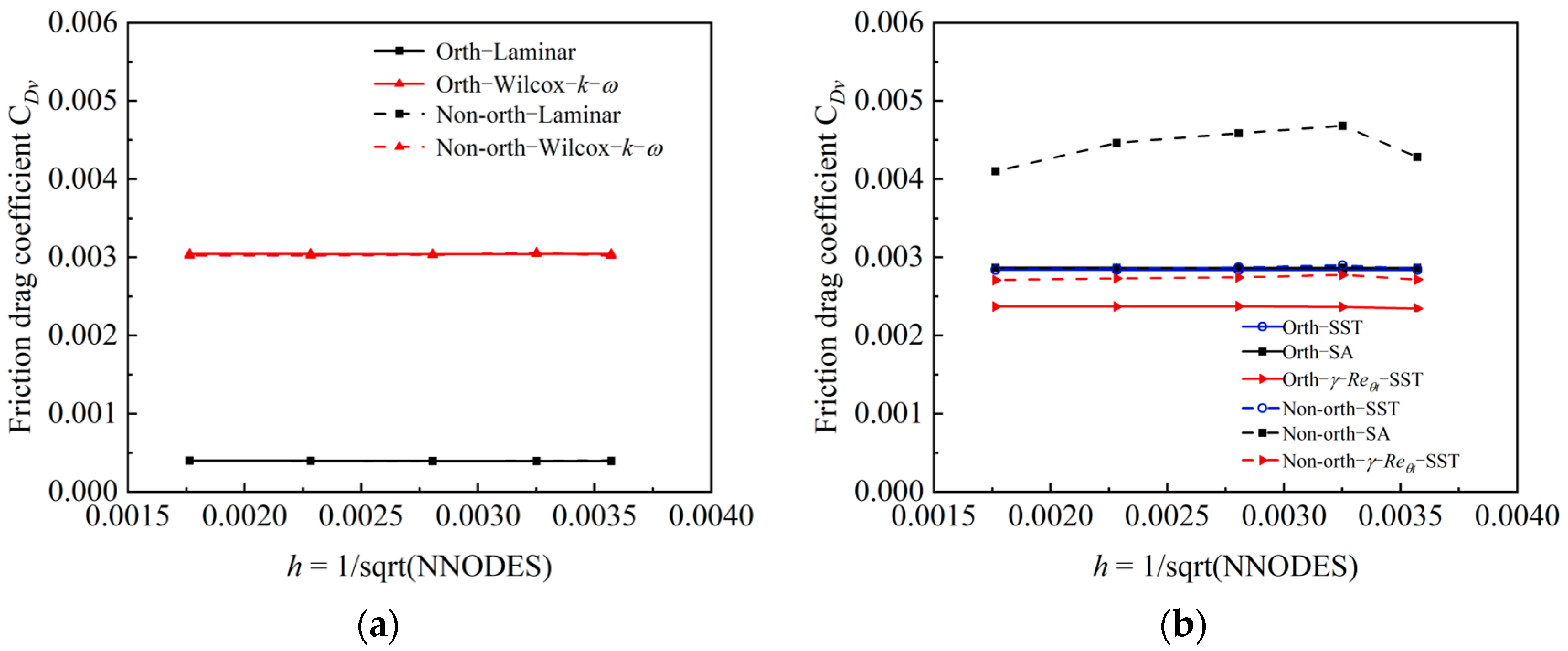
3.1.2. Mesh Convergence Analysis for All Models

In order to study the effects of mesh quantity, the orthogonal mesh and those with an oblique angle of 45° were chosen with the mesh convergence checked using five different density meshes. The basic mesh (484 × 162) used 162 points in the wall-normal direction including 121 points in the boundary layer, where the size of the first layer mesh is, and the growth rate was 1.1 in the normal direction and the y⁺ < 1 condition was kept on the wall; 484 points were used in the streamwise direction, where 262 points were on the plate, 161 points were set in the transition region at the leading edge and 101 points were used at the trailing edge. With the point setting in the normal direction unchanged, and with the mesh quantity in the streamwise direction in the trailing region increasing, the four other meshes were obtained as 584 × 162, 784 × 162, 1184 × 162 and 1984 × 162.

Figure 7 gives the situation of mesh convergence for the S-K plate case. The abscissa h is the reciprocal of the square root of the total point number and denotes the mesh density; the longitudinal coordinate is the drag coefficient. Figure 7a shows that the computational results of the laminar Navier–Stokes equation and Wilcox-k-ω model used reached the converged state and they did not change with the mesh orthogonality. Figure 7b shows the results from the SA model, SST model and γ-Re_θt-SST model. It can be found that only the SA model did not obtain the converged results with a non-orthogonal mesh and the drag values with non-orthogonal meshes were all larger than those with orthogonal meshes for the three models, wherein the drag increments from the SA and γ-Re_θt-SST models were substantial.

The velocity gradient distributions with orthogonal and non-orthogonal meshes are plotted under the laminar state in Figure 8. The two kinds of computational results were consistent, implying that the mesh orthogonality had no effect on the accuracy of the spatial discretization scheme of inviscid term in the RANS equation. Further, the Wilcox-k-ω model adopted did not include wall distance, and the friction drags obtained were nearly the same, implying that mesh orthogonality had no effect on the spatial discretization scheme of the turbulence model. The drag increments for the SA and SST models with non-orthogonal meshes as well as the upstream shift of transition location for the γ-Re_θt-SST model were induced by the mesh non-orthogonality, which led to larger values of wall distance.

Figure 9 shows the comparison of velocity profiles in the boundary layer derived from the SA model, SST model and γ-Re_θt-SST model at Re_x = 6.72 × 10⁵. It can be found that the velocity profiles in the boundary layer were basically consistent for the two kinds of mesh and SST model. With non-orthogonal meshes, the velocity profiles in the boundary layer from the SA and γ-Re_θt-SST models are more saturated relative to those with orthogonal meshes, implying that the uncertainty of wall distance has larger effects on the SA and γ-Re_θt-SST models relative to that on the SST model.

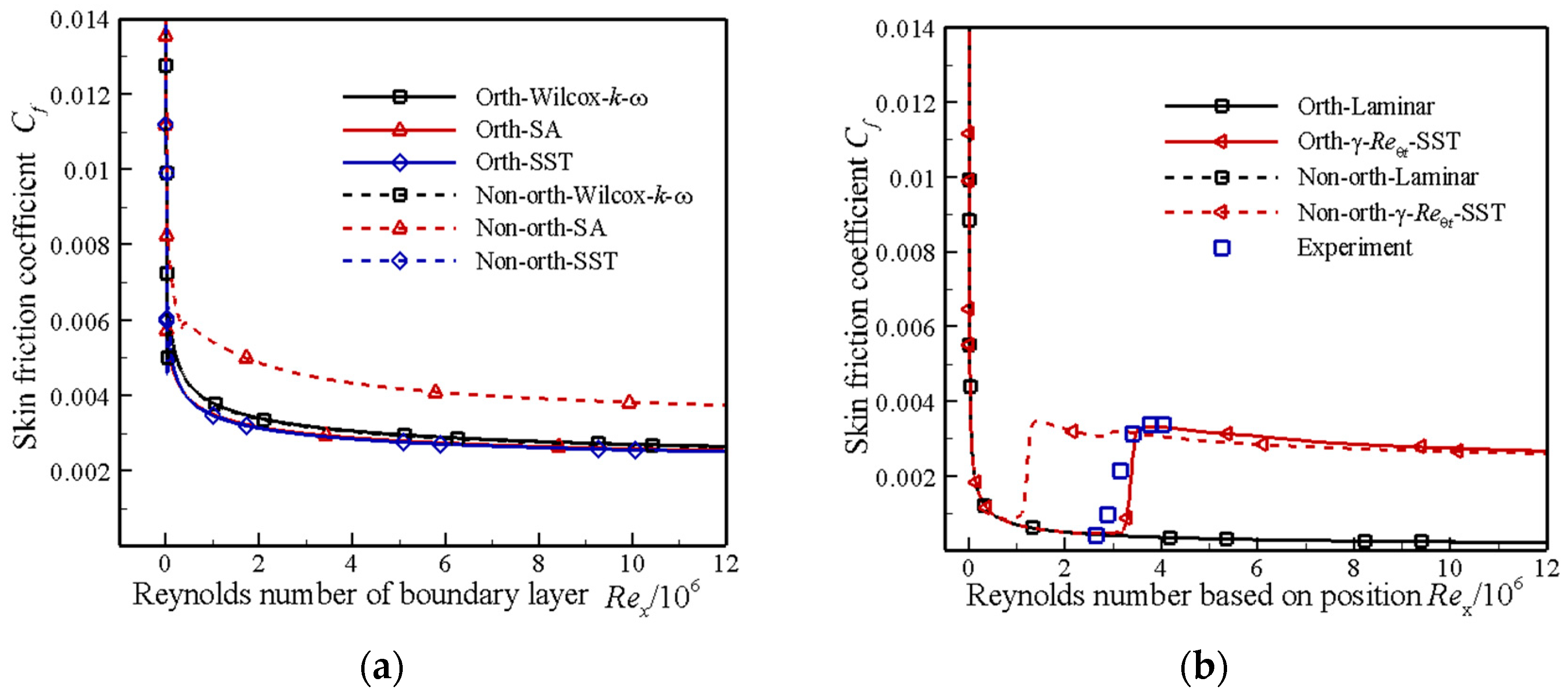
3.1.3. The Analysis of the Effects of Mesh Oblique Degree on the SA, SST and γ-Re_θt-SST Models

The friction drag distributions are shown in Figure 10 with the mesh oblique degrees ranging from 0° to 60°, where a black solid line denotes the result with the orthogonal mesh, and the dashed lines are those with non-orthogonal meshes. For the SA model depicted in Figure 10a, the friction drag with the non-orthogonal mesh was slightly larger than that with orthogonal mesh at θ = 5°. With the increasing oblique angle, the increments of friction drag from the non-orthogonal meshes increases. When θ ≥ 45°, the ‘false’ transition phenomena even arose [30]. For the SST model, the results with the oblique angle of 45° were basically consistent with those with orthogonal meshes. Thus, for the SST model, the mesh analysis was only given for large values of oblique angles (${50}^{\circ }$ and ${60}^{\circ }$), as shown in Figure 10b. The result implies that the friction drag with non-orthogonal mesh was initially enlarged when θ > 50°. Figure 10c gives the results from the γ-Re_θt-SST model. It can be found that the transition location began to shift towards the upstream direction with the increase in mesh oblique degree. When θ > 15°, the beginning location of transition was seen to shift obviously towards the upstream direction. Seen from the results relevant to the mesh oblique degree, the requirement of mesh orthogonality for the SST model was relatively low compared with the SA and γ-Re_θt-SST models, which can be explained by the model constructions. The SA model was constructed using the empirical relationship of the turbulent boundary layer, and the generation and dissipation terms in the transportation equation used wall distance directly, leading to the sensitivity of the SA model to mesh orthogonality. The SST model was a two-layer one. The inner layer used the k-ω model, the outer layer used k-ε model and this model did not contain wall distance, with wall distance used only in the construction of the layering function, while for γ-Re_θt-SST model, the wall distance was directly used to construct transition triggering function, as shown in Formula (7). Thus, it had great effects on transition location and aerodynamic force.

3.1.4. The Effects of Wall Distance Uncertainty on Transition Model

With the purpose of investigating the effects of wall distance uncertainty on the transition model, the flat plate case with the non-orthogonal mesh (1184 × 162) with an oblique angle of 45° was analyzed. The wall distance distribution is shown at Re_x = 4.03 × 10⁵ in Figure 11, where the abscissa is the ratio of actual wall distance to the thickness of the local boundary layer, the left longitudinal coordinate is the ratio of the wall distance from the direct computation method to the thickness of the local boundary layer and the right longitudinal coordinate is the local vorticity Reynolds number. The results show that at this station, the wall distance with the non-orthogonal mesh was not correct within three times of boundary layer thickness. While within two times the boundary layer thickness, the wall distance with non-orthogonal mesh satisfied a simple geometry relationship with the orthogonal mesh, as shown in Formula (10), leading to the computed vorticity Reynolds number with a non-orthogonal mesh that was two times the actual value.

$$\begin{array}{l}{\displaystyle \frac{d}{d_{\mathrm{CFD}}}}=\cos \theta \\ {\left({\mathrm{Re}}_{v,\max }\right)}_{\mathrm{Orth}}={\cos }^2\theta \times {\left({\mathrm{Re}}_{v,\max }\right)}_{\mathrm{Non}-\mathrm{orth}}\end{array}$$

(9)

Figure 12 depicts the relationship between the region of incorrect wall distance with the non-orthogonal mesh and the streamwise station, which contains the laminar region and turbulent region. It can be found that with the increasing Re_x, the thickness of the boundary layer increased. The range of the region with the computational error of wall distance relative to the boundary layer decreased, still lying in the range of the viscous sublayer and a part of the logarithmic layer and was greatly influential to the whole computation of turbulence/transition.

3.1.5. The Comparison Analysis of the Accuracy of the Turbulence Model

With the mesh quantity (1184 × 162), all turbulence models can reach mesh convergence. Now, using the orthogonal and non-orthogonal (the oblique angle is ${45}^{\circ }$) meshes with this mesh quantity, the results from different turbulence models are analyzed and compared. Figure 13a shows the comparison of friction coefficients from the Wilcox-k-ω model, SA model and SST model and Figure 13b gives the comparison of the laminar solution with that from transition model. It can be found that the friction drag coefficient with non-orthogonal mesh from the SA model increased substantially; the friction drags with orthogonal and non-orthogonal meshes from the SST model were basically consistent; and the increase in wall distance led to the upstream shift of the beginning location of transition with a large amplitude. Under the premise of the orthogonal mesh, the differences in friction coefficient distribution originated just from the turbulence model. The friction drag coefficients from the SA and SST models were close, and that from the Wilcox-k-ω model was larger.

3.2. RAE2822 Airfoil

RAE2822 airfoil [32] is a classic transonic airfoil and has several basic features of supercritical airfoil, such as the flat upper surface, the loading at the trailing edge, a relatively large curvature at the leading edge, a negative front of the camber line and a positive back [33]. This airfoil was chosen as one of the testing examples for steady transonic flow [34]. Case 9 [32] was chosen for the following study with Ma = 0.73, Re_c = 6.5 × 10⁶, c = 0.382 m, α = 2.8°. Although it is not a typical case for transition, we still used the transition model to carry out the computation of this case, to study the sensitivity of this model to mesh under moderate Reynolds numbers. The turbulence intensity from the freestream was set to decrease to the lower limit near the airfoil.

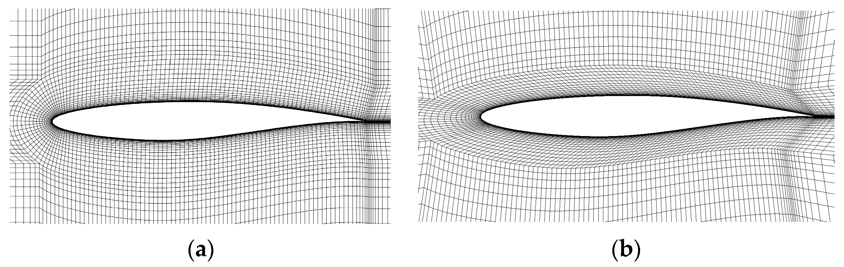
3.2.1. Mesh and Boundary Condition

The computational mesh was the structured one of C type with the streamwise farfield distance as 150c and the normal distance as 100c. The mesh spacing of the first layer was 7.65 × 10⁻⁷ m and the normal growth rate of mesh size was 1.1 in the boundary layer, ensuring that y⁺ < 1. To investigate the mesh convergence feature, six sets of mesh with different densities were used for the orthogonal and non-orthogonal meshes. Figure 14 gives the distributions of coarse mesh. It can be found that it was hard for the oblique degree of non-orthogonal mesh at the leading edge to be consistent with that at the airfoil surface, where there was a smaller oblique degree.

3.2.2. Mesh Convergence Analysis

The information of point setting for the six sets of mesh is shown in

Table 1. Mesh point information for RAE2822 airfoil.

Mesh	Total Point Number	Number on Surface	Normal Point Number
coarse	19,964	183	41
basic	41,400	271	61
fine	97,704	415	93
mildly finer	228,760	639	141
finer	524,468	979	213
finest	909,812	1495	321

, where the number on surface is the one around the airfoil, and the normal point number is the one of the nearest block in the wall-normal direction.

Figure 15 shows the mesh convergence situations for the computation with AoA (angle of attack) fixed. With increasing mesh density, the friction coefficients from the other three models except the SA model achieved the converged status, except that the converged values from different turbulence models and mesh quantities were quite different. This result implies that the effect degree of mesh orthogonality on the transonic flow problem is equivalent to that of the turbulence model.

3.2.3. The Effects of the Uncertainty of Wall Distance on the Transition Model

For representing the distributions of wall distance and vorticity Reynolds number in the boundary layer, Figure 16 gives the comparison of the distributions between the upper surface and lower surfaces at the leading edge with 979 × 213 mesh used. Due to the difference in mesh oblique degree, the difference in the computed vorticity Reynolds number with non-orthogonal mesh on the lower surface with the correct value was larger than that on the upper surface.

3.2.4. The Comparison of the Accuracy of the Turbulence Model

For comparing the abilities of turbulence models to capture the shock wave location, the aerodynamic force results with finer meshes and different models were examined carefully. The computed coefficients are given in

Table 2. Results of aerodynamic force for RAE2822 airfoil with 979 × 213 mesh.

Model	Orthogonal Mesh		Non-Orthogonal Mesh
	CD	CDv	CD	CDv
Wilcox-k-w	0.0183	0.0062	0.0185	0.0062
SST	0.0160	0.0056	0.0164	0.0060
SA	0.0175	0.0058	0.0233	0.0112
γ-Reθt-SST	0.0155	0.0028	0.0156	0.0052

, the results show that the drag value from the Wilcox-k-ω model with orthogonal mesh had a difference of 2 counts (1 count = 0.0001 of the drag coefficient) with the non-orthogonal mesh and the same friction drag. For the SST model, the difference in drag coefficient was 4 counts, while for the SA model, the drag coefficient with the non-orthogonal mesh was larger than that with orthogonal mesh by 58 counts. The drag difference from the transition model was mainly contributed by friction drag, and the difference in friction drag coefficient was about 24 counts.

The distributions of the pressure coefficient and surface friction coefficient are shown in Figure 17, where the effects of non-orthogonal mesh on the γ-Re_θt-SST model and SA model were relatively great because of the increase in wall distance. Compared with the results with orthogonal mesh, the peak value of negative pressure from the SA model was decreased with non-orthogonal mesh, the shock wave was shifted towards the upstream direction and the friction coefficients on the upper and lower surfaces at the upstream side of shock wave increased greatly. For the γ-Re_θt-SST model, the peak value of negative pressure with non-orthogonal mesh was decreased and the location of shock wave was shifted towards the upstream direction. The results of the friction coefficient show that the transition location with non-orthogonal mesh was shifted towards the upstream direction. For the SST model, the non-orthogonality of mesh had a small effect. Both the peak value of negative pressure and the location of shock wave nearly coincided with those with orthogonal mesh, except that the friction coefficients on the upper and lower surfaces had low-amplitude increments. The distributions of pressure and friction drag were not affected by the change in wall distance for the Wilcox-k-w model.

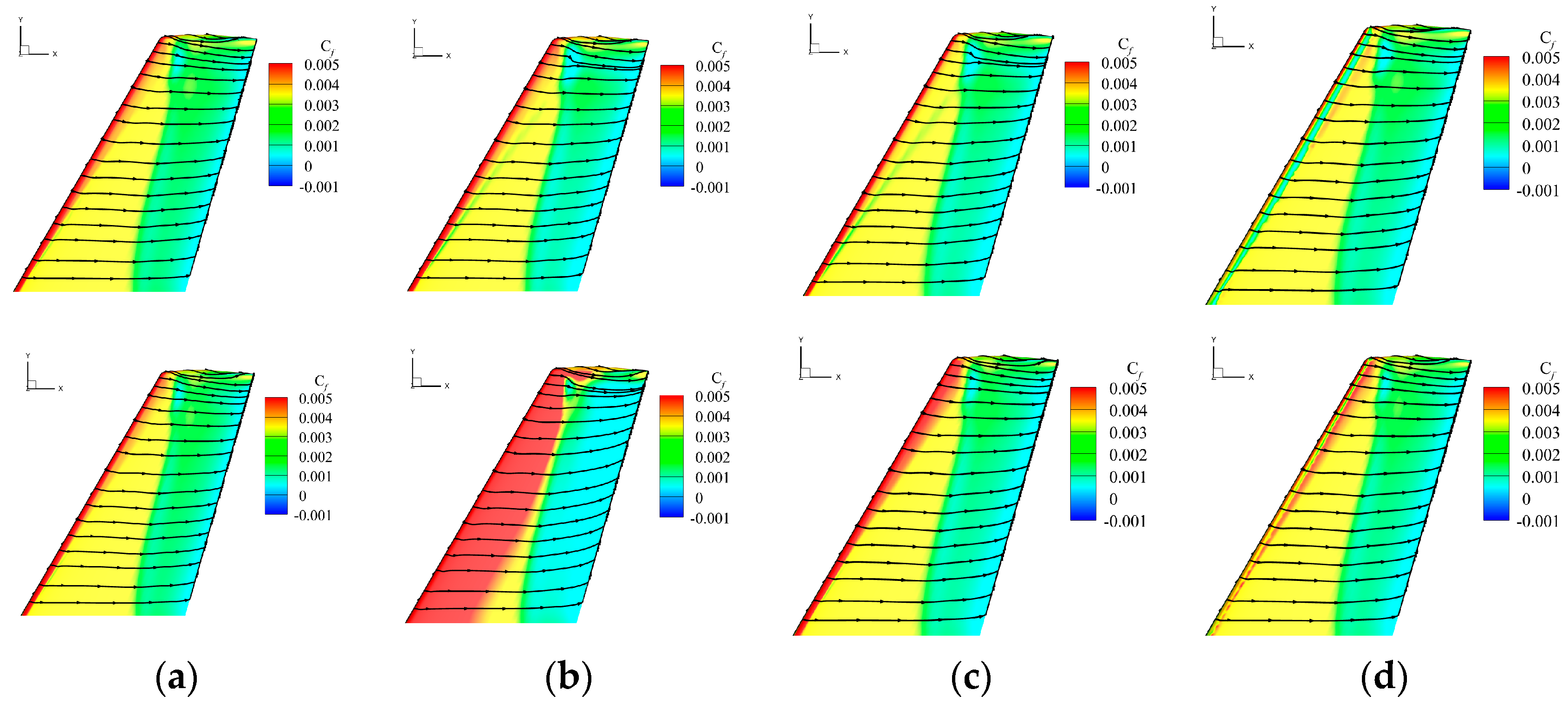
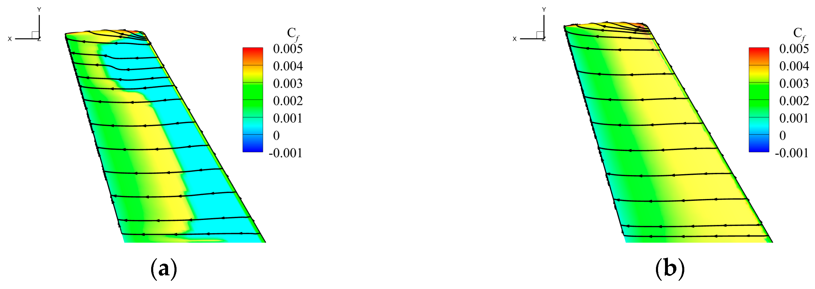
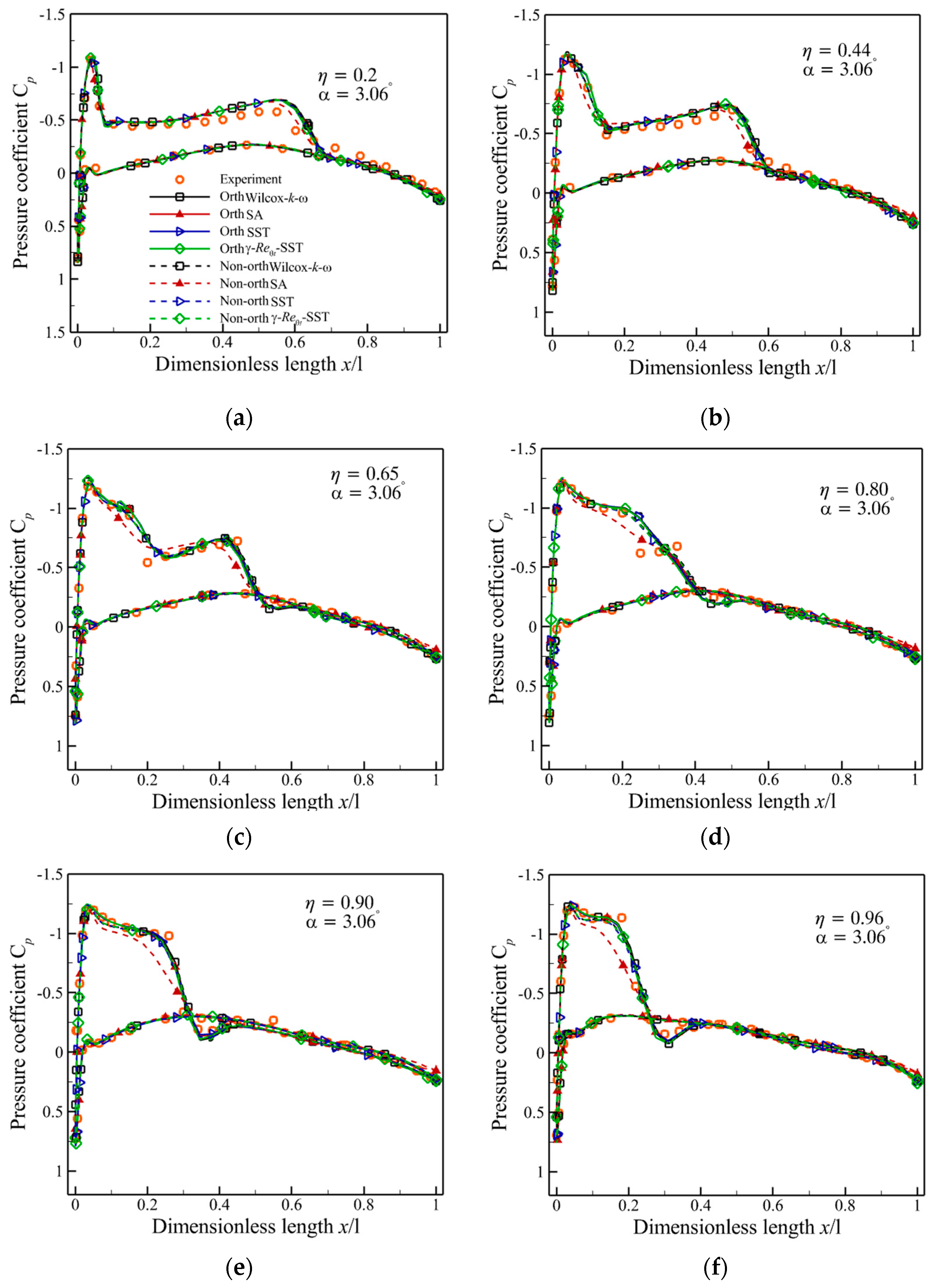
3.3. ONERA M6 Airfoil

The ONERA M6 wing is a classic three-dimensional transonic example. In the computation, the freestream Mach number is Ma = 0.8395, the Reynolds number based on the root chord is Re = 14.6 × 10⁶, and the angle of attack is α = 3.06°. Similar to the RAE2822 airfoil, this example is a common one to investigate turbulence behaviors, such as transonic shock wave, flow separation and the shock wave/boundary layer interaction. Due to the small aspect ratio, there are two shock waves on the upper surface, forming the shock wave of “λ” type at the outer section. The turbulence models including the Wilcox-k-ω model, SA model and SST model as well as γ-Re_θt-SST transition model are used to study the effects of mesh orthogonality on three-dimensional flow simulations. With transition computation considered, we aimed to study the sensitivity of the transition model containing the transportation equation with wall distance used to mesh orthogonality under the condition of a high Reynolds number. The turbulence intensity of freestream was below 0.05%.

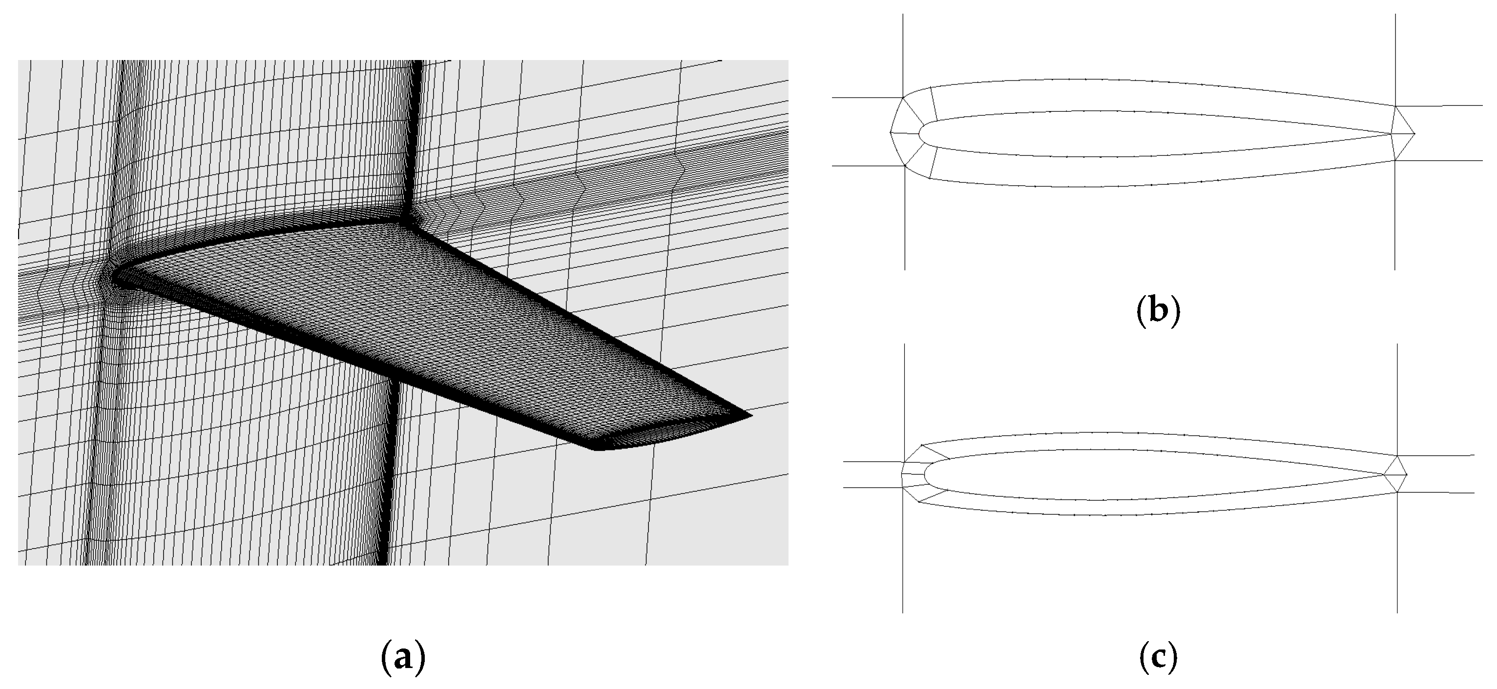
3.3.1. Mesh and Boundary Condition

The far-field of ball type was used for computation with the far-field radius as 100c. The pressure field boundary was set at the far-field, the symmetry boundary was set at the root boundary, and the viscous wall boundary was set for the wing surface. Figure 18 depicts the block splitting, for which the points on the slice near the wing root were adjusted to be on the same plane as that for the points on the slice near the wingtip. The so-called orthogonal mesh can only ensure that the mesh on the slice is a two-dimensional orthogonal mesh. Due to the swept wing with a root-tip-ratio larger than 1, the slices were not perpendicular to the wing surface. As the computational cost was large for three-dimensional configurations, the coarse mesh with the mesh scale close to RAE2822 was chosen. The total number of mesh points was about 2,800,000, with 174 points set in the streamwise direction and 61 points set in the normal direction in the near blocks. The height of the first layer mesh was 1.9 × 10⁻⁶ m.

3.3.2. The Effects of Wall Distance Uncertainty on the Transition Model

As mentioned above, the complete orthogonal mesh was hard to obtain for three-dimensional configurations based on the ‘block to block’ strategy, and most meshes close to the walls were oblique. The results of wall distance and the vorticity Reynolds number on the upper surface at Re_s = 4.01 × 10⁵ and on the lower surface at Re_s = 3.14 × 10⁵ are shown in Figure 19. The above locations lie in the laminar region at the leading edge. The results show that the wall distances with non-orthogonal meshes were incorrect within the range of six times of boundary layer thickness, wherein the vorticity Reynolds number was about three times of that with orthogonal mesh. Compared with the cases of the two-dimensional airfoil and flat plate, the difference in wall distance due to non-orthogonal mesh was larger for three-dimensional configurations. The reasons for the larger differences in wall distance and vorticity Reynolds number due to non-orthogonal mesh include three aspects: (1) the mesh density near the surface was relatively small; (2) the presented station was near the leading edge with a large oblique angle of non-orthogonal mesh; (3) the Reynolds number considered was relatively large with a thin boundary layer, and the near-wall mesh of high quality was hard to obtain using the ‘block to block’ strategy.

3.3.3. The Comparison of the Uncertainties of the Turbulence Models

Table 3. Results of ONERA M6 model with orthogonal grid and non-orthogonal grid.

Model	Orthogonal Mesh		Non-Orthogonal Mesh
	CD	CDv	CD	CDv
Wilcox-k-ω	0.0177	0.0057	0.0177	0.0056
SST	0.0170	0.0052	0.0174	0.0055
SA	0.0175	0.0055	0.0231	0.0099
γ-Reθt-SST	0.0155	0.0044	0.0173	0.0054

gives the drag results with orthogonal and non-orthogonal meshes for the ONERA M6 wing. The drag coefficients with the two meshes from the Wilcox-k-ω model were consistent, and the difference in friction drag coefficient was about 1 count. The difference in total drag coefficient from the SST model was about 4 counts, and that for the SA model reached 56 counts. The drag coefficient with non-orthogonal mesh from the transition model was larger than that with orthogonal mesh by 18 counts.

Figure 20 gives the contours of surface friction coefficient on the upper surface from different models and different mesh orthogonality. The results on the lower surface are shown in Figure 21 from the γ-Re_θt-SST model. The difference in friction drag coefficient from the Wilcox-k-ω model was not obvious. For the SA model, the surface friction coefficient with non-orthogonal mesh was greatly larger than that with orthogonal mesh before the shock wave, and the trend was opposite after the shock wave. The region featured by high friction coefficient with non-orthogonal mesh for the SST model lies between the leading edge and the first shock wave. The results from the transition model show that with orthogonal mesh, there is a laminar region on the upper surface at the upstream side of the first shock wave and the lower surface has a larger range of laminar region. Nevertheless, the distribution of friction drag with non-orthogonal mesh was nearly the same as that from the SST model.

Figure 22 shows the pressure distributions at several stations for the ONERA M6 wing. It can be found that the results with non-orthogonal mesh from the SA model had great differences with the experimental results. The negative pressure on the suction surface was obviously smaller than those from other models, and the location of the second shock wave was at the upstream side of those from other models. The results from other models were relatively consistent with the experimental results, having small potential differences in the peak value of negative pressure and the location of shock wave. At η = 0.20, the locations of shock wave from all models were at the downstream of that from the experimental results. At η = 0.80, the two shock waves were seen to combine together for all models, different from the experimental results. At η = 0.90 and η = 0.96, the locations of shock wave from all models were at the upstream side of that in the experiment results.

In general, with orthogonal mesh, the changes in the peak value of suction force at the leading edge and the location of shock wave were minor with the changing turbulence model. With non-orthogonal mesh, the peak value of negative pressure had a small effect on the pressure distribution and shock wave. For the SST model, the difference in pressure distribution due to the change in mesh orthogonality was comparable with that due to the change from the SST model to the Wilcox-k-ω model. However, the simulation results of the SA model and transition model relied highly on the mesh.

4. Conclusions

The effects of mesh orthogonality on the numerical results are investigated systematically in this paper for the laminar equation, SA model, SST model, Wilcox-k-ω model and γ-Re_θt-SST model. The cases of the S-K flat plate, RAE2822 airfoil and ONERA M6 wing are analyzed and several sets of non-orthogonal mesh with different oblique degrees are used for the S-K flat plate. The main conclusions are as follows:

The wall distance derived by the direct computation method is affected by the mesh orthogonality. For non-orthogonal mesh, its value is relevant to the streamwise distance and the oblique degree of mesh.

Seen from the case of the flat plate, the results from the Wilcox-k-ω model do not rely on the mesh orthogonality. The results with non-orthogonal mesh from the SA model cannot reach the converged state and have large differences with those with orthogonal mesh, which increase with the increase in the oblique degree of mesh; the results from the γ-Re_θt-SST model can reach the converged state. The transition location with non-orthogonal mesh lies forward and the effect of the oblique degree on transition location is great; the requirement of the SST model on mesh orthogonality is not high. Nevertheless, the large oblique degree may lead to a larger friction drag.

For transonic flows, the shock wave behavior is dominant, the suction force at the leading edge and the location of shock wave may change slightly with the turbulence model. The SA model yields poor results with non-orthogonal mesh. Wilcox-k-ω is not affected by the mesh orthogonality. The SST model is slightly sensitive to the mesh orthogonality in terms of suction peak, shock location as well as surface friction. For aeronautic problems, the SST model is highly recommended.

For the γ-Re_θt-SST transition model, the oblique mesh may lead to the substantial upstream shift of the beginning location of transition, as the vorticity Reynolds number in this transition model includes the square of wall distance. For the configurations, such as airfoils and wings with a high Reynolds number, the transition phenomena may even occur near the leading edge, if the mesh orthogonality is bad at the leading edge. This conclusion is suitable for all transition models using the transportation equation with the vorticity Reynolds number.

References

1. Slotnick, J.; Khodadoust, A.; Alonso, J.; Darmofal, D.; Gropp, W.; Lurie, E.; Mavriplis, D.J. CFD Vision 2030 Study: A Path to Revolutionary Computational Aerosciences: NASA/CR-20414-218178; NASA: Washington, DC, USA, 2014.
2. Yan, C.; Qu, F.; Zhao, Y.T.; Yu, J.; Wu, C.H.; Zhang, S.H. Review of development and challenges for physical modeling and numerical scheme of CFD in aeronautics and astronautics. Acta Aerodyn. Sin. 2020, 38, 829–857. (In Chinese) [Google Scholar]
3. Cary, A.W.; Chawner, J.R.; Duque, E.P.N.; Gropp, W.; Kleb, W.L.; Kolonay, R.M.; Nielsen, E.; Smith, B. CFD vision 2030 roadmap: Progress and perspectives. In Proceedings of the AIAA Aviation 2021 Forum, Virtual Event, 2–6 August 2021; American Institute of Aeronautics and Astronautics: Reston, VI, USA, 2021. [Google Scholar]
4. Piomelli, U. Large-eddy simulation: Achievements and challenges. Prog. Aerosp. Sci. 1999, 35, 335–362. [Google Scholar] [CrossRef]
5. Yang, Z.Y. Large-eddy simulation: Past, present and the future. Chin. J. Aeronaut. 2015, 28, 11–24. [Google Scholar]
6. Moser, R.D.; Haering, S.W.; Yalla, G.R. Statistical properties of subgrid-scale turbulence models. Annu. Rev. Fluid Mech. 2021, 53, 255–286. [Google Scholar] [CrossRef]
7. Spalart, P.R. Detached-eddy simulation. Annu. Rev. Fluid Mech. 2008, 41, 181–202. [Google Scholar] [CrossRef]
8. Durbin, P.A. Some recent developments in turbulence closure modeling. Annu. Rev. Fluid Mech. 2018, 50, 77–103. [Google Scholar] [CrossRef]
9. He, X.; Zhao, F.; Vahdati, M. Detached eddy simulation: Recent development and application to compressor tip leakage flow. J. Turbomach. 2021, 144, 011009. [Google Scholar] [CrossRef]
10. Zhang, K.L.; Li, S.Y.; Duan, Y.; Yan, C. Uncertainty quantification of parameters in SST turbulence model for inlet simulation. Acta Aeronaut. Astronaut. Sin. 2023, 44, 729429. (In Chinese) [Google Scholar]
11. Chen, J.T.; Zhang, C.; Wu, X.J.; Zhao, W. Quantification of turbulence model-selection uncertainties considering discretization errors. Acta Aeronaut. Astronaut. Sin. 2021, 42, 625741. (In Chinese) [Google Scholar]
12. Zhao, Y.T.; Liu, H.K.; Zhou, Q.; Yan, C. Quantification of parametric uncertainty in k–ωγ transition model for hypersonic flow heat transfer. Aerosp. Sci. Technol. 2020, 96, 105553. [Google Scholar] [CrossRef]
13. Zhao, Y.T.; Yan, C.; Liu, H.K.; Zhang, K. Uncertainty and sensitivity analysis of flow parameters for transition models on hypersonic flows. Int. J. Heat Mass Transf. 2019, 135, 1286–1299. [Google Scholar] [CrossRef]
14. Xiao, H.; Cinnella, P. Quantification of model uncertainty in RANS simulations: A review. Prog. Aerosp. Sci. 2019, 108, 1–31. [Google Scholar] [CrossRef]
15. Spalart, P.; Allmaras, S. A one-equation turbulence model for aerodynamic flows. In Proceedings of the 30th Aerospace Sciences Meeting and Exhibit, Reston, NV, USA, 6–9 January 1992; AIAA: Reston, VI, USA, 1992. [Google Scholar]
16. Menter, F.R.; Kuntz, M.; Langtry, R. Ten years of industrial experience with the SST turbulence model. Turbul. Heat Mass Transf. 2003, 4, 625–632. [Google Scholar]
17. Langtry, R.B.; Menter, F.R. Correlation-based transition modeling for unstructured parallelized computational fluid dynamics codes. AIAA J. 2009, 47, 2894–2906. [Google Scholar] [CrossRef]
18. Wilcox, D.C. Reassessment of the scale-determining equation for advanced turbulence models. AIAA J. 1988, 26, 1299–1310. [Google Scholar] [CrossRef]
19. Tucker, P.G.; Rumsey, C.L.; Spalart, P.R.; Bartels, R.E.; Biedron, R.T. Computations of wall distances based on differential equations. AIAA J. 2005, 43, 539–549. [Google Scholar] [CrossRef]
20. Xu, J.L.; Yan, C.; Fan, J.J. Computations of wall distances by solving a transport equation. Appl. Math. Mech. 2011, 32, 135–143. (In Chinese) [Google Scholar] [CrossRef]
21. Wang, G.; Zeng, Z.; Ye, Z.Y. An efficient search algorithm for calculating minimum wall distance of unstructured mesh. Northwestern Polytech. Univ. 2014, 32, 511–516. (In Chinese) [Google Scholar]
22. Zhao, H.Y.; He, X.Z.; Le, J.L. Recursive box method for wall distance computation. Chin. J. Comput. Phys. 2008, 25, 427–430. (In Chinese) [Google Scholar]
23. Meng, S.; Zhou, D.; Li, X.L.; Bi, L. Accurate and efficient wall distance calculation method for Cartesian grids. Acta Aerodyn. Sin. 2023, 41, 93–101. (In Chinese) [Google Scholar]
24. Zhao, Z.; He, L.; Zhang, J.; Xu, Q.; Zhang, L. MPI/OpenMP hybrid parallel computation of wall distance for turbulence flow simulations. Acta Aerodyn. Sin. 2019, 37, 883–892. (In Chinese) [Google Scholar]
25. Rumsey, C. The Splart-Allmaras Turbulence Model [EB/OL]. Available online: https://turbmodels.larc.nasa.gov/spalart.html (accessed on 23 July 2023).
26. Rumsey, C. Turbulence Modeling Resource [EB/OL]. Available online: https://turbmodels.larc.nasa.gov/ (accessed on 23 July 2023).
27. Nie, S.Y.; Wang, Y.; Liu, Z.Q.; Jin, P.; Jiao, J. Numerical inverstigation and discussion on CHN-T1 benchmark model using Spalart-Allmaras model and SSG/LRR-w model. Acta Aerodyn. Sin. 2019, 37, 310–319, 328. (In Chinese) [Google Scholar]
28. Schubauer, G.B.; Klebanoff, P.S. Contributions on the mechanics of boundary-layer transition. Tech. Rep. Arch. Image Libr. 1956, 39, 411–415. [Google Scholar]
29. He, S.T.; Lan, W.; Hu, X.J. Numerical simulation of flow pattern structure in boundary layer on flat plate surfaces. J. South China Univ. Technol. (Nat. Sci. Ed.) 2021, 49, 9–18. (In Chinese) [Google Scholar]
30. Spalart, P.R.; Rumsey, C.L. Effective inflow conditions for turbulence models in aerodynamic calculations. AIAA J. 2007, 45, 2544–2553. [Google Scholar] [CrossRef]
31. Shi, Y.Y.; Bai, J.Q.; Hua, J.; Yang, T.H. Transition prediction based on amplification factor and Spalart-Allmaras turbulence model. J. Aerosp. Power 2015, 30, 1670–1677. (In Chinese) [Google Scholar]
32. Cook, P.H.; Mcdonald, M.A.; Firmin, M.C.P. Aerofoil RAE2822-pressure distributions, and boundary layer and wake measurements. In Experimental Data Base for Computer Program Assessment; AGARD AR-138; 1979; Available online: https://www.sto.nato.int/publications/AGARD/AGARD-AR-138/AGARD-AR-138.pdf (accessed on 22 October 2024).
33. Bai, W. Analyses of wind-tunnel test data of the transonic airfoil RAE2822. Acta Aerodyn. Sin. 2023, 41, 55–70. (In Chinese) [Google Scholar]
34. Dervieux, A.; Braza, M.; Dussauge, J.P. Computation and Comparison of Efficient Turbulence Models for Aeronautics—European Research Project ETMA; Notes on Numerical Fluid Mechanics; Vieweg: Wiesbaden, Germany, 1998. [Google Scholar]
35. Schmitt, V.; Charpin, F. Pressure Distributions on the ONERA M6-Wing at Transonic Mach Numbers. AGARD AR-138. 1979. Available online: https://www.semanticscholar.org/paper/Pressure-distributions-on-the-ONERA-M6-wing-at-Mach-Schmitt-Charpin/6498e2b6c38d7da95a07fe539bbf8525eba8f730 (accessed on 9 November 2023).
Figure 1. Sketch of different approaches to obtain the minimum distance to the nearest wall (taken from Ref. [25]).
Aerospace 11 00898 g001
Figure 2. Geometric relations of minimum wall distance for orthogonal and non-orthogonal meshes.
Aerospace 11 00898 g002
Figure 3. The variation of the minimum nearest distance of the non-orthogonal mesh wall along the normal direction of the object surface.
Aerospace 11 00898 g003
Figure 4. Comparison of wall distances of non-orthogonal grids of different densities at the same station.
Aerospace 11 00898 g004
Figure 5. Sketch of boundary conditions for S-K flat plate.
Aerospace 11 00898 g005
Figure 6. Grid topology for orthogonal and non-orthogonal grids.
Aerospace 11 00898 g006
Figure 7. Grid convergence behavior of drag coefficient for S-K flat plate. (a) Laminar solution, Wilcox k-ω model; (b) SST, SA and γ-Reθt-SST models.
Aerospace 11 00898 g007
Figure 8. Velocity gradient profile of laminar solution.
Aerospace 11 00898 g008
Figure 9. Comparison of velocity profile at Rex = 6.72 × 10⁵.
Aerospace 11 00898 g009
Figure 10. Results of grid sensitivity analysis. (a) SA model; (b) SST model; (c) γ-Reθt-SST model.
Aerospace 11 00898 g010
Figure 11. Comparison of wall distance vs. vorticity Reynolds number at Rex = 4.03 × 10⁵.
Aerospace 11 00898 g011
Figure 12. Results of calculated wall distance on non-orthogonal grid at different positions.
Aerospace 11 00898 g012
Figure 13. Comparison of forces computed by different turbulence models. (a) The comparison of laminar solution with those from SA and SST models; (b) the comparison of laminar solution with that from γ-Reθt-SST model as well as the experimental data taken from Ref [31].
Aerospace 11 00898 g013
Figure 14. Grid topology of RAE2822 airfoil. (a) Orthogonal mesh; (b) non-orthogonal mesh.
Aerospace 11 00898 g014
Figure 15. Mesh convergence results of friction drag coefficient for RAE2822 airfoil.
Aerospace 11 00898 g015
Figure 16. Sketch of wall distance and vorticity Reynolds number results for RAE2822. (a) Res = 2.04 × 10⁵ upper surface; (b) Res = 2.64 × 10⁵ lower surface.
Aerospace 11 00898 g016
Figure 17. Comparison of force coefficients for RAE2822 airfoil with experimental data from Ref [29]. (a) The pressure distribution with orthogonal mesh; (b) the pressure distribution with non-orthogonal mesh; (c) friction drag distribution with the orthogonal mesh; (d) friction drag distribution with the non-orthogonal mesh.
Aerospace 11 00898 g017
Figure 18. Grid topology of the ONERA M6 wing. (a) The surface mesh for ONERA M6 wing; (b) the splitting of the orthogonal mesh at the symmetry plane for the ONERA M6 wing; (c) the splitting of the non-orthogonal mesh at the symmetry plane for the ONERA M6 wing.
Aerospace 11 00898 g018
Figure 19. Sketch of wall distance and vorticity Reynolds number results for ONERA M6 wing. (a) The upper surface, Res = 4.01 × 10⁵; (b) the lower surface, Res = 3.14 × 10⁵.
Aerospace 11 00898 g019
Figure 20. Distributions of skin friction coefficient using orthogonal (up) and non-orthogonal (down) meshes on upper surfaces by different turbulence models. (a) Wilcox-k-ω; (b) SA; (c) SST; (d) γ-Reθt-SST.
Aerospace 11 00898 g020
Figure 21. Distributions of skin friction coefficient computed by γ-Reθt-SST model using orthogonal (left) and non-orthogonal meshes on lower surfaces. (a) Orthogonal mesh; (b) non-orthogonal mesh.
Aerospace 11 00898 g021
Figure 22. Pressure coefficient at each section for ONERA M6 wing, the experimental data is taken from Ref [35]. (a) η = 0.2; (b) η = 0.44; (c) η = 0.65; (d) η = 0.80; (e) η = 0.90; (f) η = 0.96.
Aerospace 11 00898 g022