Identification of High-Order Linear Time-Invariant Models from Periodic Nonlinear System Responses ^†

Abstract

This paper presents a novel step in the extension of subspace identification toward the direct identification of harmonic decomposition linear time-invariant models from nonlinear time-periodic system responses. The proposed methodology is demonstrated through examples involving the nonlinear time-periodic dynamics of a flapping-wing micro aerial vehicle. These examples focus on the identification of the vertical dynamics from various types of input–output data, including linear time-invariant, linear time-periodic, and nonlinear time-periodic input–output data. A harmonic analyzer is used to decompose the linear time-periodic and nonlinear time-periodic responses into harmonic components and introduce spurious dynamics into the identification, which make the identified model order selection challenging. A similar effect is introduced by measurement noise. The use of model order reduction and model-matching methods in the identification process is studied to recover the harmonic decomposition structure of the known system. The identified models are validated in the frequency and time domains.

1. Introduction

Systems with periodic dynamics exist across multiple engineering disciplines, with examples including, but not limited to, bio-inspired robots (e.g., insects, birds, fish), spacecraft, rotorcraft, wind turbines, jet engines, and communication systems. The dynamics of these systems are generally represented by nonlinear time-periodic systems (NLTPs). A significant body of methods and tools is already available for the identification of linear time-periodic (LTP) systems and their linear time-invariant (LTI) reformulations from linear systems’ responses, but a number of significant issues remain in the identification of LTP systems and their LTI reformulations from nonlinear responses. This is especially true for challenging applications in which time periodicity is associated with multivariable, nonlinear, and high-order dynamics. Because aerospace vehicles with time-periodic dynamics such as rotorcraft and flapping-wing flyers/micro aerial vehicles (MAVs) are indeed characterized by multivariable, nonlinear, and high-order dynamics, the development of new methodologies is key for assessing their dynamic stability and for performing flight control design.

A considerable amount of literature exists on the extraction of LTP systems and their LTI reformulations from NLTP systems via numerical schemes. In rotorcraft applications, LTP systems and their linear time-invariant (LTI) reformulations are relevant to the prediction of vibratory/rotor loads and to the analysis and design of active rotor control systems. A comprehensive survey of active rotor control system approaches can be found in Ref. [1]. Furthermore, LTI reformulations of LTP systems enabled the study of the interference effects between the higher harmonic control (HHC) and the aircraft flight control system (AFCS) in maneuvering flights [2,3,4,5]. Recently, LTI reformulations of LTP systems were employed in the design of load alleviation control (LAC) laws [6,7]. A comprehensive survey of the methods used to extract harmonically decomposed LTI models of rotorcraft can be found in Ref. [8]. In flapping-wing applications, LTI reformulations of LTP systems are important for the study of dynamic stability. Methods span averaging methods [9,10,11], Floquet theory (Refs. [12,13,14,15]), and harmonic decomposition (Refs. [16,17]).

All of these methods, however, are focused on the extraction of LTI reformulations of LTP systems from physics-based models via numerical schemes, rather than from system identification. In fact, only a limited number of studies have sought to identify the LTP dynamics of rotorcraft or flapping-wing vehicles. For rotorcraft LTP system identification, see Ref. [8] and the references therein. For flapping-wing vehicles, see Refs. [18,19,20]. Surprisingly, to the best of the knowledge of the authors, very little published work exists which is focused on the direct identification of harmonic decomposition LTI models for any of these vehicles. It is important to point out that the application of time-invariant reformulations to convert an LTP model identification problem into an LTI one is far from straightforward because of the need to define an approach to return the LTI identified model to its LTP counterpart. To handle this difficulty, as well as to simplify the application of model identification in Multi-Input Multi-Output (MIMO) LTP systems, periodic extensions of subspace model identification methods have been developed over the last few years. Early works in this direction include the LTP extensions of the intersection algorithm [21] and of the Multivariable Output Error State sPace (MOESP) algorithm [22,23] and the approach in Ref. [24]. In Ref. [25], an approach towards Linear Parameter Varying (LPV) model identification subject to the requirement of a periodic scheduling sequence has been proposed. In recent years novel approaches towards the subspace identification of LTP systems have been proposed, both in the time domain and in the frequency domain using harmonic transfer functions (see, e.g., Refs. [26,27,28,29,30,31]).

As such, the objective of this paper is to extend the use of the subspace identification of higher-order LTI systems in harmonic decomposition form from nonlinear time-periodic (NLTP) system responses, as presented in our previous work [32]. Unlike existing methods, our approach employs system identification directly on the harmonically decomposed signals of the NLTP response to analyze the dynamics of the nonlinear test data. To the best of the authors’ knowledge, this methodology has not been previously explored. It introduces new challenges in the application of identification techniques, such as the emergence of spurious dynamics and issues with model matching, which are addressed in this paper.

The paper begins with a detailed description of the proposed methodology and the mathematical background. The methodology is demonstrated through examples involving the NLTP dynamics of a flapping-wing micro aerial vehicle (FWMAV). The examples focus on the identification of the FWMAV dynamics from various types of input–output data, including LTI, LTP, and NLTP input–output data. The effect of a harmonic analyzer in decomposing the LTP and NLTP responses into harmonics is assessed for the identification process, along with the effect of measurement noise. The identified models are validated in both the frequency and time domains.

2. Methodology

2.1. Mathematical Background

Consider a nonlinear time-periodic (NLTP) system in first-order form:

$$\begin{array}{cc}\hfill \dot{\mathit{x}}& =\mathit{f}\left(\mathit{x},\mathit{u},t\right)\hfill \end{array}$$

(1a)

$$\begin{array}{cc}\hfill \mathit{y}& =\mathit{g}\left(\mathit{x},\mathit{u},t\right)\hfill \end{array}$$

(1b)

where $\mathit{x}\in {\mathbb{R}}^n$ is the state vector, $\mathit{u}\in {\mathbb{R}}^m$ is the control input vector, $\mathit{y}\in {\mathbb{R}}^l$ is the output vector, and t is the dimensional time in seconds. The nonlinear functions $\mathit{f}$ and $\mathit{g}$ are T-periodic in time such that:

$$\begin{array}{cc}\hfill \mathit{f}(\mathit{x},\mathit{u},t)& =\mathit{f}(\mathit{x},\mathit{u},t+T)\hfill \end{array}$$

(2a)

$$\begin{array}{cc}\hfill \mathit{g}(\mathit{x},\mathit{u},t)& =\mathit{g}(\mathit{x},\mathit{u},t+T)\hfill \end{array}$$

(2b)

Note that the fundamental period in the system is $T={\displaystyle \frac{2\pi }{\omega }}$ s, where $\omega$ is the frequency of excitation in rad/s. Let ${\mathit{x}}^{\ast }\left(t\right)$ and ${\mathit{u}}^{\ast }\left(t\right)$ represent a periodic solution of the system such that ${\mathit{x}}^{\ast }\left(t\right)={\mathit{x}}^{\ast }(t+T)$ and ${\mathit{u}}^{\ast }\left(t\right)={\mathit{u}}^{\ast }(t+T)$.

Let ${\mathit{x}}^{\ast }\left(t\right)$ and ${\mathit{u}}^{\ast }\left(t\right)$ represent a periodic solution of the system such that ${\mathit{x}}^{\ast }\left(t\right)={\mathit{x}}^{\ast }(t+T)$ and ${\mathit{u}}^{\ast }\left(t\right)={\mathit{u}}^{\ast }(t+T)$. Then, the NLTP system can be linearized about the periodic solution. Consider the case of small disturbances:

$$\begin{array}{cc}\hfill \mathit{x}& ={\mathit{x}}^{\ast }+\mathsf{\Delta }\mathit{x}\hfill \end{array}$$

(3a)

$$\begin{array}{cc}\hfill \mathit{u}& ={\mathit{u}}^{\ast }+\mathsf{\Delta }\mathit{u}\hfill \end{array}$$

(3b)

where $\mathsf{\Delta }\mathit{x}$, and $\mathsf{\Delta }\mathit{u}$ are the state and control perturbation vectors from the candidate periodic solution. A Taylor series expansion is performed on the state derivative and output vectors. Neglecting terms higher than the first order results in the following equations:

$$\begin{array}{c}\hfill \mathit{f}\left({\mathit{x}}^{\ast }+\mathsf{\Delta }\mathit{x},{\mathit{u}}^{\ast }+\mathsf{\Delta }\mathit{u},t\right)=\mathit{f}\left({\mathit{x}}^{\ast },{\mathit{u}}^{\ast },t\right)\mathit{F}\left(t\right)\mathsf{\Delta }\mathit{x}+\mathit{G}\left(t\right)\mathsf{\Delta }\mathit{u}\end{array}$$

(4a)

$$\begin{array}{c}\hfill \mathit{g}\left({\mathit{x}}^{\ast }+\mathsf{\Delta }\mathit{x},{\mathit{u}}^{\ast }+\mathsf{\Delta }\mathit{u},t\right)=\mathit{g}\left({\mathit{x}}^{\ast },{\mathit{u}}^{\ast },t\right)\mathit{P}\left(t\right)\mathsf{\Delta }\mathit{x}+\mathit{Q}\left(t\right)\mathsf{\Delta }\mathit{u}\end{array}$$

(4b)

where:

$$\begin{array}{cc}\hfill \mathbf{F}\left(t\right)& ={\displaystyle \frac{\partial \mathbf{f}\left(\mathbf{x},\mathbf{u}\right)}{\partial \mathbf{x}}}{|}_{\begin{array}{c}{\mathbf{x}}^{\ast },{\mathbf{u}}^{\ast }\end{array}},\hfill \end{array}$$

(5a)

$$\begin{array}{cc}\hfill \mathbf{G}\left(t\right)& ={\displaystyle \frac{\partial \mathbf{f}\left(\mathbf{x},\mathbf{u}\right)}{\partial \mathbf{u}}}{|}_{\begin{array}{c}{\mathbf{x}}^{\ast },{\mathbf{u}}^{\ast }\end{array}},\hfill \end{array}$$

(5b)

$$\begin{array}{cc}\hfill \mathbf{P}\left(t\right)& ={\displaystyle \frac{\partial \mathbf{g}\left(\mathbf{x},\mathbf{u}\right)}{\partial \mathbf{x}}}{|}_{\begin{array}{c}{\mathbf{x}}^{\ast },{\mathbf{u}}^{\ast }\end{array}},\hfill \end{array}$$

(5c)

$$\begin{array}{cc}\hfill \mathbf{Q}\left(t\right)& ={\displaystyle \frac{\partial \mathbf{g}\left(\mathbf{x},\mathbf{u}\right)}{\partial \mathbf{u}}}{|}_{\begin{array}{c}{\mathbf{x}}^{\ast },{\mathbf{u}}^{\ast }\end{array}}\hfill \end{array}$$

(5d)

Note that the state–space matrices in Equations (5a), (5b), (5c) and (5d) have T-periodic coefficients. Equations (4a) and (4b) yield a linear time-periodic (LTP) approximation of the NLTP system of Equations (1a) and (1b) as follows:

$$\begin{array}{c}\hfill \mathsf{\Delta }\dot{\mathit{x}}=\mathit{F}\left(t\right)\mathsf{\Delta }\mathit{x}+\mathit{G}\left(t\right)\mathsf{\Delta }\mathit{u}\end{array}$$

(6a)

$$\begin{array}{c}\hfill \mathsf{\Delta }\mathit{y}=\mathit{P}\left(t\right)\mathsf{\Delta }\mathit{x}+\mathit{Q}\left(t\right)\mathsf{\Delta }\mathit{u}\end{array}$$

(6b)

Hereafter, the notation is simplified by dropping the $\mathsf{\Delta }$ in front of the linearized perturbation state and control vectors while keeping in mind that these vectors represent perturbations from a periodic equilibrium. Next, the state, input, and output vectors of the LTP systems are decomposed into a finite number of harmonics of the fundamental period via Fourier analysis:

$$\begin{array}{c}\hfill \mathit{x}={\mathit{x}}_0+\sum _{i=1}^N{\mathit{x}}_{ic}cosi\psi +{\mathit{x}}_{is}sini\psi \end{array}$$

(7a)

$$\begin{array}{c}\hfill \mathit{u}={\mathit{u}}_0+\sum _{j=1}^M{\mathit{u}}_{jc}cosj\psi +{\mathit{u}}_{js}sinj\psi \end{array}$$

(7b)

$$\begin{array}{c}\hfill \mathit{y}={\mathit{y}}_0+\sum _{k=1}^L{\mathit{y}}_{kc}cosk\psi +{\mathit{y}}_{ks}sink\psi \end{array}$$

(7c)

where the subscript ₀ refers to the average (or mean) component of the respective variable, while the subscripts _ic, _jc, _kc and _is, _js, _ks denote the ith, jth, and kth harmonic cosine and sine components of x, u, and y, respectively.

As shown in Ref. [16], the harmonic decomposition methodology can be used to transform the LTP model into an approximate higher-order linear time-invariant (LTI) model in the first-order form:

$$\begin{array}{c}\hfill \dot{\mathit{X}}=\mathit{A}\mathit{X}+\mathit{B}\mathit{U}\end{array}$$

(8a)

$$\begin{array}{c}\hfill \mathit{Y}=\mathit{C}\mathit{X}+\mathit{D}\mathit{U}\end{array}$$

(8b)

where the augmented state, control, and output vectors are:

$$\begin{array}{cc}\hfill {\mathit{X}}^T& =\left[{\mathit{x}}_0^T{\mathit{x}}_{1c}^T{\mathit{x}}_{1s}^T\dots {\mathit{x}}_{Nc}^T{\mathit{x}}_{Ns}^T\right]\hfill \end{array}$$

(9a)

$$\begin{array}{cc}\hfill {\mathit{U}}^T& =\left[{\mathit{u}}_0^T{\mathit{u}}_{1c}^T{\mathit{u}}_{1s}^T\dots {\mathit{u}}_{Mc}^T{\mathit{u}}_{Ms}^T\right]\hfill \end{array}$$

(9b)

$$\begin{array}{cc}\hfill {\mathit{Y}}^T& =\left[{\mathit{y}}_0^T{\mathit{y}}_{1c}^T{\mathit{y}}_{1s}^T\dots {\mathit{y}}_{Lc}^T{\mathit{y}}_{Ls}^T\right]\hfill \end{array}$$

(9c)

with $\mathit{A}\in {\mathbb{R}}^{n(2N+1)\times n(2N+1)}$, $\mathit{B}\in {\mathbb{R}}^{n(2N+1)\times m(2M+1)}$, $\mathit{C}\in {\mathbb{R}}^{l(2L+1)\times n(2N+1)}$, and $\mathit{D}\in {\mathbb{R}}^{l(2L+1)\times m(2M+1)}$.

2.2. Subspace Identification

Consider now a discrete-time representation of the harmonic decomposition system in Equations (8a) and (8b) with unknown coefficient matrices:

$$\begin{array}{c}\mathit{X}[k+1]={\mathit{A}}_d\mathit{X}\left[k\right]+{\mathit{B}}_d\mathit{U}\left[k\right]\end{array}$$

(10a)

$$\begin{array}{c}\mathit{Y}\left[k\right]=\mathit{C}\mathit{X}\left[k\right]+\mathit{D}\mathit{U}\left[k\right]\end{array}$$

(10b)

where the subscript d strands for discrete. This system represents the approximate LTI dynamics to be identified.

For this, subspace identification is used. The choice of subspace identification is justified by its single-step approach to solving for the unknown system coefficients, as opposed to an iterative process. Here, a discrete-time approach to identification is adopted as the Hankel matrices constructed from input-output data with continuous-time methods may become ill-conditioned for high-order systems because of their block Vandermonde structure [33]. Because the systems considered in this study may be of a high order, depending on the number of harmonics of interest, discrete-time subspace identification offers increased numerical stability. Based on this framework, the identification problem is stated as follows: given s measurements of input $\mathit{U}\left[k\right]$ and output $\mathit{Y}\left[k\right]$ generated by the unknown system in Equations (1a) and (1b) and then decomposed to its harmonics using a harmonic analyzer, determine the order of the unknown system (i.e., $n(2N+1)$) and the coefficient matrices ${\mathit{A}}_d$, ${\mathit{B}}_d$, $\mathit{C}$, and $\mathit{D}$ up to a similarity transformation. The general procedure of the subspace identification algorithm is summarized from Refs. [23,34,35] and is articulated in five major steps.

The first step involves the construction of the block Hankel matrices from the given input-output data. The input block Hankel matrices are defined as:

$$\begin{array}{cc}\hfill {\mathit{U}}_{\mathrm{block}}& =\left[\begin{array}{c}\begin{array}{ccccc}{\mathit{U}}_1& {\mathit{U}}_2& {\mathit{U}}_3& \cdots & {\mathit{U}}_j\\ {\mathit{U}}_2& {\mathit{U}}_3& {\mathit{U}}_4& \cdots & {\mathit{U}}_{j+1}\\ ⋮& ⋮& ⋮& \ddots & ⋮\\ {\mathit{U}}_i& {\mathit{U}}_{i+1}& {\mathit{U}}_{i+2}& \cdots & {\mathit{U}}_{i+j-1}\\ ine{\mathit{U}}_{i+1}& {\mathit{U}}_{i+2}& {\mathit{U}}_{i+3}& \cdots & {\mathit{U}}_{i+j}\\ {\mathit{U}}_{i+2}& {\mathit{U}}_{i+3}& {\mathit{U}}_{i+4}& \cdots & {\mathit{U}}_{i+j+1}\\ ⋮& ⋮& ⋮& \ddots & ⋮\\ {\mathit{U}}_{2i}& {\mathit{U}}_{2i+1}& {\mathit{U}}_{2i+2}& \cdots & {\mathit{U}}_{2i+j-1}\end{array}\end{array}\right]=\left[\begin{array}{c}\begin{array}{c}{\mathit{U}}_p\\ ine{\mathit{U}}_f\end{array}\end{array}\right]\hfill \end{array}$$

(11)

where the subscripts p and f indicate past and future data, respectively, i is the number of block rows, and j is the number of block columns. The number of block rows i is arbitrarily chosen such that it is larger than the order of the system and $j=s-2i+1$. In Ref. [23], i is recommended to be equal to twice the ratio between the maximum order and the number of outputs. The output block Hankel matrices ${\mathit{Y}}_p$, and ${\mathit{Y}}_f$ are found in a similar way. Note that in Equation (11). past data correspond to rows up to the ith, whereas future data correspond to rows after the ith. By applying recursive substitution to Equations (10a) and (10b), one obtains

$$\begin{array}{c}\hfill {\mathit{Y}}_p={\mathsf{\Gamma }}_i{\mathit{X}}_p+{\mathbf{H}}_i{\mathit{U}}_p\end{array}$$

(12a)

$$\begin{array}{c}\hfill {\mathit{Y}}_f={\mathsf{\Gamma }}_i{\mathit{X}}_f+{\mathit{H}}_i{\mathit{U}}_f\end{array}$$

(12b)

where the observability matrix is defined as:

$${\mathsf{\Gamma }}_i={\left[\begin{array}{ccccc}\mathit{C}& \mathit{C}{\mathit{A}}_d& \mathit{C}{\mathit{A}}_d^2& \cdots & \mathit{C}{\mathit{A}}_d^{i-1}\end{array}\right]}^T$$

(13)

The matrix ${\mathit{H}}_i$ is a block Toeplitz matrix of the following form:

$${\mathit{H}}_i=\left[\begin{array}{ccccc}\mathit{D}& \mathbf{0}& \cdots & \cdots & \mathbf{0}\\ \mathit{C}{\mathit{B}}_d& \mathit{D}& \mathbf{0}& \cdots & \mathbf{0}\\ \mathit{C}{\mathit{A}}_d{\mathit{B}}_d& \mathit{C}{\mathit{B}}_d& \mathit{D}& \cdots & \mathbf{0}\\ ⋮& ⋮& ⋮& \ddots & ⋮\\ \mathit{C}{\mathit{A}}_d^{i-2}{\mathit{B}}_d& \mathit{C}{\mathit{A}}_d^{i-3}{\mathit{B}}_d& \cdots & \mathit{C}{\mathit{B}}_d& \mathit{D}\end{array}\right]$$

(14)

Additionally, the past and future states are stacked states defined as

$$\begin{array}{c}\hfill {\mathit{X}}_p=\left[\begin{array}{cccc}{\mathit{X}}_0& {\mathit{X}}_1& \cdots & {\mathit{X}}_{i-1}\end{array}\right]\end{array}$$

(15a)

$$\begin{array}{c}\hfill {\mathit{X}}_f=\left[\begin{array}{cccc}{\mathit{X}}_i& {\mathit{X}}_{i+1}& \cdots & {\mathit{X}}_{i+j-1}\end{array}\right]\end{array}$$

(15b)

The second step involves the computation of the oblique projection by means of QR decomposition. In this step, the projection of the future output space along the future input space into the joint space of the past input and output ( ${{\mathit{Y}}_f}_{/{\mathit{U}}_f}\left({\displaystyle \genfrac{}{}{0pt}{}{{\mathit{U}}_p}{{\mathit{Y}}_p}}\right)$) is found. This projection can be thought of as the problem of predicting the future outputs ${\mathit{Y}}_f$ using the information obtained from the past data $\left({\displaystyle \genfrac{}{}{0pt}{}{{\mathit{U}}_p}{{\mathit{Y}}_p}}\right)$, and the knowledge of the future inputs ${\mathit{U}}_f$. Then, the observability matrix ${\mathsf{\Gamma }}_i$ is extracted from this projection by means of singular-value decomposition (Ref. [23]).

In the third step, the singular value decomposition of the weighted oblique projection is computed. In this step, the order of the system is determined as the number of non-zero singular values. In practice, the order of the system is found by comparing the singular values with a small threshold greater than zero. In step four, the shift property of the observability matrix is used to obtain the identified system and output matrices ${\mathit{A}}_d$ and $\mathit{C}$. In step five, the control and feedthrough matrices ${\mathit{B}}_d$ and $\mathit{D}$ are calculated using the least square method. Lastly, the identified system is transformed back to continuous-time form.

2.3. Model-Order Reduction

Because system identification is performed for a harmonic decomposition model, input–output data from the NLTP system need to be decomposed into harmonics of the fundamental frequency of the system. To carry this out, the input–output data are processed with a harmonic analyzer to extract the harmonic coefficients of the signal. This has the adverse effect of introducing spurious dynamics into the identification. To remove these spurious dynamics from the identified system, model order reduction is employed. Those spurious dynamics introduced that are relatively slow compared to the known fundamental frequency of the system are first removed via truncation. The states corresponding to these dynamics are typically identified through a spectral analysis of the identified system. However, some prior knowledge of the system is required to understand which dynamics are indeed spurious. Next, those spurious dynamics that are faster than the fundamental frequency are removed using singular perturbation theory [36]. More specifically, under the assumption that the identified dynamics are stable, residualization is used to further reduce the order of the model [36].

The state vector of identified dynamics is partitioned into fast and slow components:

$${\mathit{X}}^T=\left[{\mathit{X}}_{\mathrm{s}}^T{\mathit{X}}_{\mathrm{f}}^T\right]$$

(16)

Then, the identified dynamics can be re-written as

$$\left[\begin{array}{c}{\dot{\mathit{X}}}_{\mathrm{s}}\\ {\dot{\mathit{X}}}_{\mathrm{f}}\end{array}\right]=\left[\begin{array}{cc}{\mathit{A}}_{\mathrm{s}}\hfill & {\mathit{A}}_{\mathrm{sf}}\hfill \\ {\mathit{A}}_{\mathrm{fs}}\hfill & {\mathit{A}}_{\mathrm{f}}\hfill \end{array}\right]\left[\begin{array}{c}{\mathit{X}}_{\mathrm{s}}\hfill \\ {\mathit{X}}_{\mathrm{f}}\hfill \end{array}\right]+\left[\begin{array}{c}{\mathit{B}}_{\mathrm{s}}\hfill \\ {\mathit{B}}_{\mathrm{f}}\hfill \end{array}\right]\mathit{U}$$

(17)

By neglecting the dynamics of the fast states i.e., $\left.{\dot{\mathit{X}}}_{\mathrm{f}}=0\right)$ and performing a few algebraic manipulations, the equations for a reduced-order system with the state vector composed of the slow states is

$${\dot{\mathit{X}}}_{\mathrm{s}}=\widehat{\mathit{A}}{\mathit{X}}_{\mathrm{s}}+\widehat{\mathit{B}}\mathit{U}$$

(18)

where

$$\begin{array}{c}\hfill \widehat{\mathit{A}}={\mathit{A}}_{\mathrm{s}}-{\mathit{A}}_{\mathrm{sf}}{\mathit{A}}_{\mathrm{f}}^{-1}{\mathit{A}}_{\mathrm{fs}}\end{array}$$

(19a)

$$\begin{array}{c}\hfill \widehat{\mathit{B}}={\mathit{B}}_{\mathrm{s}}-{\mathit{A}}_{\mathrm{sf}}{\mathit{A}}_{\mathrm{f}}^{-1}{\mathit{B}}_{\mathrm{f}}\end{array}$$

(19b)

2.4. Model Matching

Because subspace identification yields an unstructured system, the states of the identified system do not generally have a physical meaning. In addition, the identified system will, in general, not be in the harmonic decomposition form. However, when the system dynamics are know a priori, the physical meaning of the states can be recovered as the identified system matrices are within a similarity transformation matrix of the harmonic decomposition model (Ref. [37]). Consider the identified unstructured dynamics in continuous time:

$$G_c:\left\{\begin{array}{c}\dot{\mathit{X}}=\mathit{A}\mathit{X}+\mathit{B}\mathit{u}\hfill \\ \mathit{Y}=\mathit{C}\mathit{X}+\mathit{D}\mathit{U}\hfill \end{array}\right.$$

(20)

Additionally, consider a structured model with unknown coefficients $\mathit{\theta }$.

$$G_s\left(\mathit{\theta }\right):\left\{\begin{array}{c}\dot{\mathit{x}}=\mathit{A}\left(\mathit{\theta }\right)\mathit{x}+\mathit{B}\left(\mathit{\theta }\right)\mathit{u}\hfill \\ \mathit{y}=\mathit{C}\left(\mathit{\theta }\right)\mathit{x}+\mathit{D}\left(\mathit{\theta }\right)\mathit{u}\hfill \end{array}\right.$$

(21)

The model matching problem consists of finding those unknown coefficients that minimize the $H_{\infty }$ norm of the difference between $G_c$ and $G_s$. Formally,

$${\mathit{\theta }}^{\ast }=\arg \min \left|\right|G_c\left(s\right)-G_s(s;\theta ){\left|\right|}_{\infty }$$

(22)

This minimization problem is a non-convex non-smooth optimization problem. This problem can be reformulated as a structured control problem for which robust computational techniques are available [38].

2.5. Summary

In summary, the proposed methodology for the direct identification of LTI harmonic decomposition models is articulated in five major steps:

• The generation of the input–output data from the NLTP system.
• Processing the input–output data with a harmonic analyzer to extract the harmonics of the fundamental frequency of the system.
• Application of subspace identification to identify the higher-order LTI dynamics.
• Removal of spurious higher-order dynamics introduced by the harmonic analyzed via model order reduction.
• Application of model-matching methods to recover the harmonic decomposition form of the identified LTI approximation to the NLTP system.

3. Simulation Model

The efficacy of the proposed methodology is demonstrated through examples involving the dynamics of a flapping-wing micro aerial vehicle (FWMAV). Consider the NLTP vertical dynamics of a FWMAV in Ref. [10]:

$$\left[\begin{array}{c}\dot{w}\\ \ddot{\varphi }\end{array}\right]=\left[\begin{array}{c}g-k_{d_1}\left|\dot{\varphi }\right|w-k_L{\dot{\varphi }}^2\\ -k_{d_2}\left|\dot{\varphi }\right|\dot{\varphi }-k_{d_3}w\dot{\varphi }\end{array}\right]+\left[\begin{array}{c}0\\ {\displaystyle \frac{1}{I_f}}cos\omega t\end{array}\right]U$$

(23)

where w is the vertical speed, $\dot{\varphi }$ is the wing flapping speed, and g is the gravitational acceleration. Additionally, $k_{d_1}$, $k_{d_2}$, $k_{d_3}$, and $k_L$ are constant parameters, $I_F$ is the flapping moment of inertia, $\omega$ is the flapping frequency, and U is the amplitude of the flapping control input. The state vector is ${\mathit{x}}^T=\left[w\varphi \right]$ and the control vector is $\mathit{u}=\left[U\right]$. A high-order LTI approximation to the NLTP dynamics at hover is found using the harmonic balance algorithm described in Refs. [17,39]. The state and control input harmonics retained in this process are up to the first order (i.e., N = 1 and M = 1). It follows that the higher-order LTI system has the following state and control input vectors:

$$\begin{array}{c}{\mathit{X}}^T=\left[w_0{\dot{\varphi }}_0{w}_{1c}{\dot{\varphi }}_{1c}{w}_{1s}{\dot{\varphi }}_{1s}\right]\end{array}$$

(24a)

$$\begin{array}{c}{\mathit{U}}^T=\left[U_0{U}_{1c}{U}_{1s}\right]\end{array}$$

(24b)

where the state and input vectors have dimensions of $n(2N+1)=6$ and $m(2M+1)=3$, respectively. The numerical values of the system parameters are taken from Ref. [10], and result in the following model:

$$\begin{array}{c}\left[\begin{array}{c}{\dot{w}}_0\\ {\ddot{\varphi }}_0\\ {\dot{w}}_{1c}\\ {\ddot{\varphi }}_{1c}\\ {\dot{w}}_{1s}\\ {\ddot{\varphi }}_{1s}\end{array}\right]=\left[\begin{array}{cccccc}-4& 0& 0& -0.032& 0& -0.105\\ 0& -75.51& -428.4& 0& -1.408\times {10}^3& 0\\ 0& -0.065& -2.892& 0& -165.9& 0\\ -856.9& 0& 0& -54.74& 0& -179.4\\ 0& -0.211& 164.5& 0& -5.107& 0\\ -2.817\times {10}^3& 0& 0& 151.0& 0& -96.28\end{array}\right]\left[\begin{array}{c}{w}_0\\ {\dot{\varphi }}_0\\ w_{1c}\\ {\dot{\varphi }}_{1c}\\ w_{1s}\\ {\dot{\varphi }}_{1s}\end{array}\right]\hfill \\ \hfill +\left[\begin{array}{ccc}0& 0& 0\\ 0& 3.628\times {10}^6& 0\\ 0& 0& 0\\ 7.256\times {10}^6& 0& 0\\ 0& 0& 0\\ 0& 0& 0\end{array}\right]\left[\begin{array}{c}{U}_0\\ U_{1c}\\ U_{1s}\end{array}\right]\end{array}$$

(25)

The state vector is rearranged to show the existence of two uncoupled subsystems:

$$\begin{array}{c}\left[\begin{array}{c}{\dot{w}}_0\\ {\ddot{\varphi }}_{1c}\\ {\ddot{\varphi }}_{1s}\\ {\ddot{\varphi }}_0\\ {\dot{w}}_{1c}\\ {\dot{w}}_{1s}\end{array}\right]=\left[\begin{array}{cccccc}-4& -0.032& -0.105& 0& 0& 0\\ -856.9& -54.747& -179.46& 0& 0& 0\\ -2.817\times {10}^3& 151.0& -96.28& 0& 0& 0\\ 0& 0& 0& -75.51& -428.4& -1.408\times {10}^3\\ 0& 0& 0& -0.065& -2.892& -165.9\\ 0& 0& 0& -0.211& 164.5& -5.107\end{array}\right]\left[\begin{array}{c}{w}_0\\ {\dot{\varphi }}_{1c}\\ {\dot{\varphi }}_{1s}\\ {\dot{\varphi }}_0\\ w_{1c}\\ w_{1s}\end{array}\right]\hfill \\ \hfill +\left[\begin{array}{ccc}0& 0& 0\\ 7.256\times {10}^6& 0& 0\\ 0& 0& 0\\ 0& 3.628\times {10}^6& 0\\ 0& 0& 0\\ 0& 0& 0\end{array}\right]\left[\begin{array}{c}{U}_0\\ U_{1c}\\ U_{1s}\end{array}\right]\end{array}$$

(26)

The zeroth harmonic of the vertical speed, $w_0$, is coupled with the first-harmonic states of the flapping speed, ${\dot{\varphi }}_{1c}$ and ${\dot{\varphi }}_{1s}$). These states are decoupled from the remaining three states (i.e., ${\dot{\varphi }}_0$, $w_{1c}$, and $w_{1s}$), which are in turn coupled together. The zeroth harmonic of the control input is shown to affect the first subsystem only, whereas the first cosine harmonic of the control input affects solely the second subsystem. To better understand the dynamic properties of each subsystem, the modal participation factors are computed [40] and are shown in Figure 1. Figure 1a shows that the vertical speed contributes to the heave mode exclusively through its zeroth harmonic, whereas its first harmonic contributes to the flap mode. On the other hand, Figure 1b shows that the flapping speed contributes to the heave mode with its first harmonics, and to the flap mode solely through its zeroth harmonic. The heave mode has a base eigenvalue of $-3.53$, whereas the flap mode has a base eigenvalue of $-75.75$. These results indicate significant frequency separation and modal participation between the two modes. Based on these considerations, the subsystem consisting of $w_0$, ${\dot{\varphi }}_{1c}$ and ${\dot{\varphi }}_{1s}$ will be identifiable by perturbing the system through the zeroth harmonic of the control input, and by measuring the response of the zeroth harmonic of the vertical speed and the first harmonic of the flapping speed. Conversely, the other subsystem which includes ${\dot{\varphi }}_0$, $w_{1c}$ and $w_{1s}$ will be identifiable by perturbing the system through the first cosine harmonic of the control input and by measuring the response of the first harmonic of the vertical speed and the zeroth harmonic of the flapping speed.

4. Results

The efficacy of the proposed methodology is demonstrated through examples involving the FWMAV dynamic model described above. These examples focus the identification of the subsystem corresponding to the heave dynamics from various types of input–output data. First, identification is performed by directly using the input–output data collected from the harmonic decomposition model (i.e., the high-order LTI model). Note that these data are already decomposed into harmonics. Next, the perturbation response corresponding to the LTP system states is reconstructed from the LTI input–output data using Equation (7c). A harmonic analyzer is applied to re-extract the harmonic coefficients of the reconstructed input–output data. These data are then used in the identification process. This is carried out to assess the effect of the harmonic analyzer on the identification process. Next the identification is repeated by applying the harmonic analyzer directly to the LTP input-output data. The process is repeated with white noise applied to the identification data to simulate measurement noise. Lastly, the proposed identification method is applied to the input–output data gathered from the NLTP system. The identification process uses the MOESP algorithm (Ref. [23]).

4.1. Identification from LTI Input-Output Data

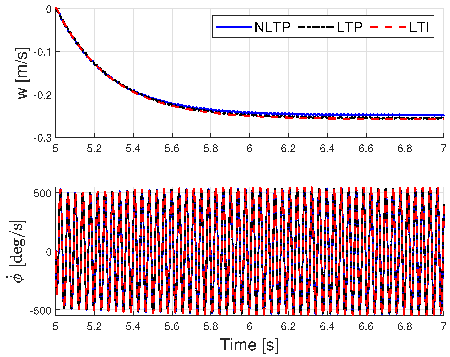
As a first example, the proposed identification method is applied to input–output data obtained using the harmonic decomposition model in Equations (25) and (26). This case is chosen first as the input–data are already decomposed into harmonics of the fundamental frequency of the system. In practical terms, the system is perturbed in its zeroth-harmonic input $U_0$ with a doublet starting at $t=5$ s and the resulting responses of $w_0$, ${\dot{\varphi }}_{1c}$, and ${\dot{\varphi }}_{1s}$ are measured. The LTI system’s response is shown in Figure 2 with a red dashed line.

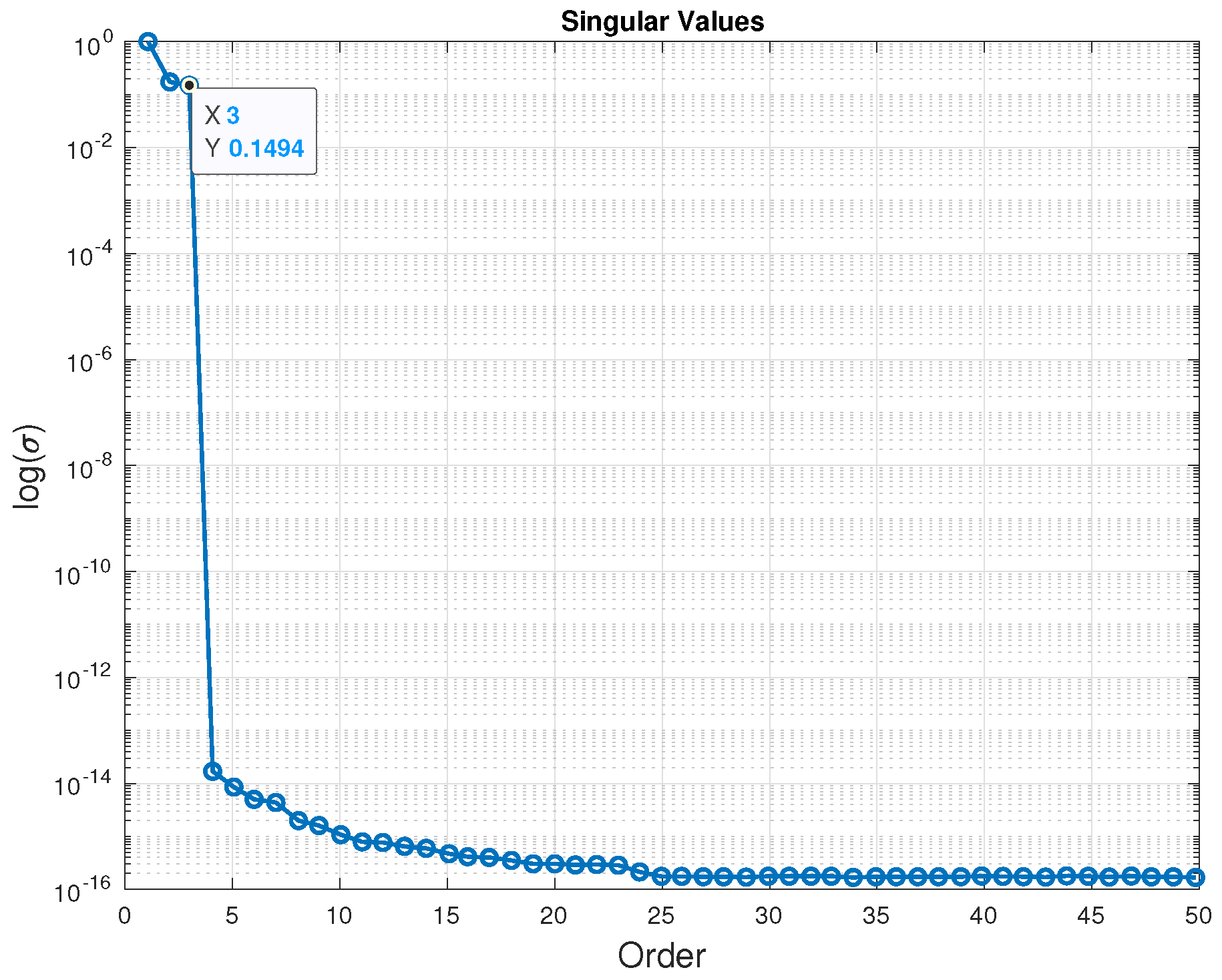
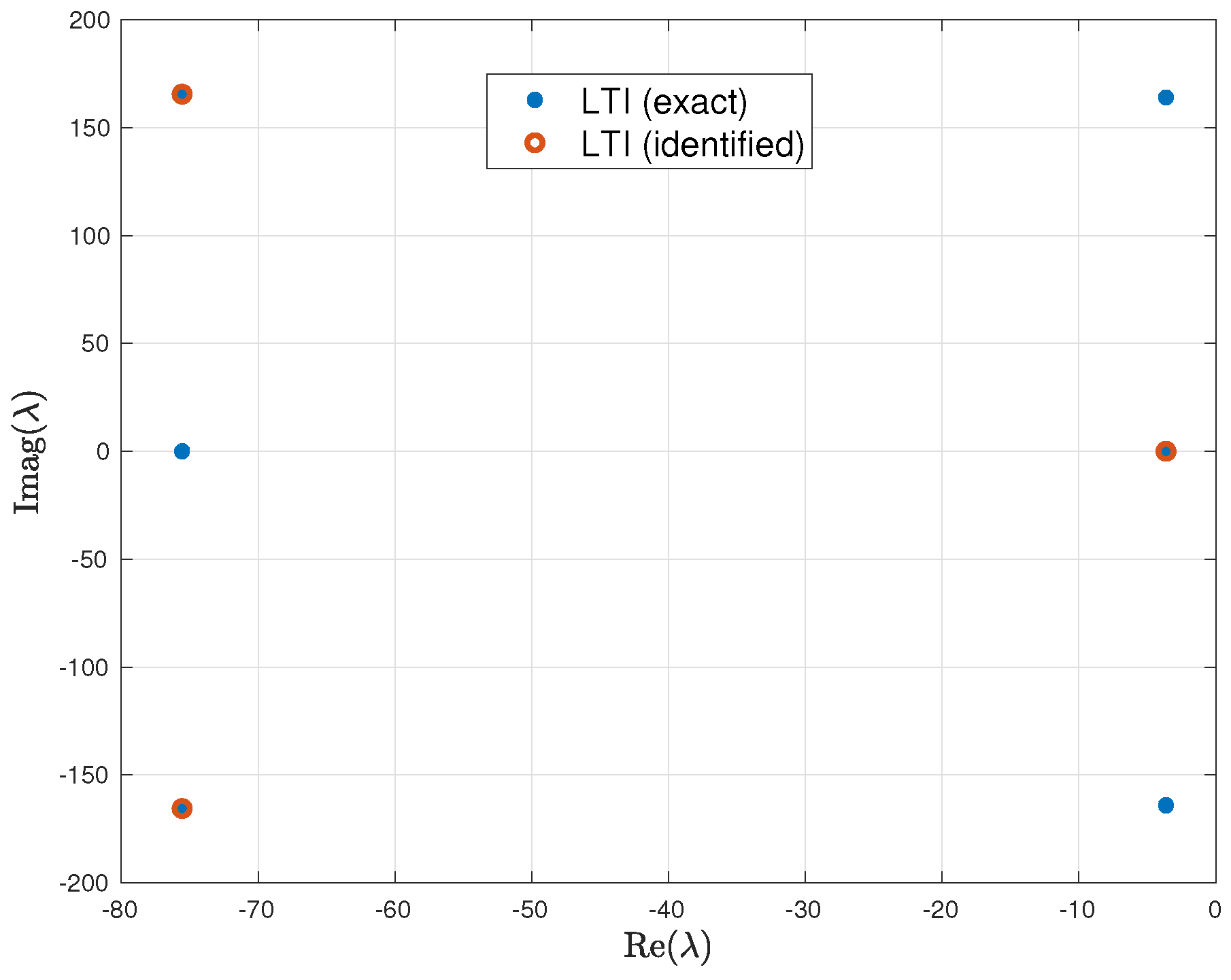
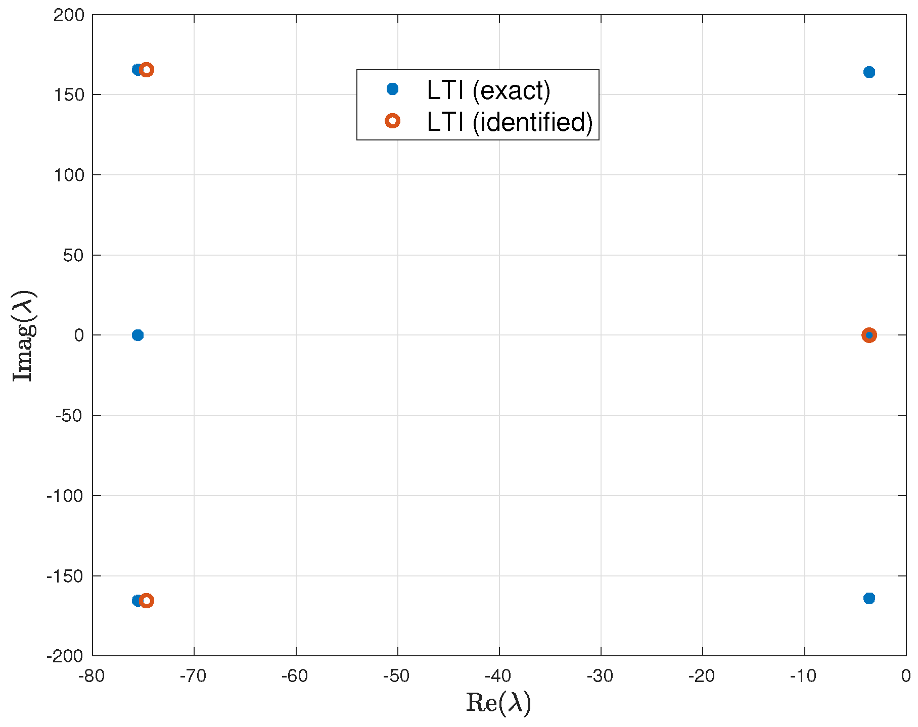
The singular values resulting from the SVD of the oblique projection are shown in Figure 3. One can see a clear gap after the third singular value, showing that only three harmonic states are controllable, thus identifiable, when using the zeroth harmonic input. The eigenvalues of the identified system are shown in Figure 4. The identified eigenvalues match well with those of the heave dynamics subsystem.

It is worth noting that, in reality, the state/output measurements are not readily decomposed into harmonics of the fundamental frequency of the system. It follows that a harmonic analyzer must be used to recover the harmonic coefficients of the input–output data. In the special case just considered in which the harmonic coefficients are readily available, the harmonic analyzer was assumed to be perfect.

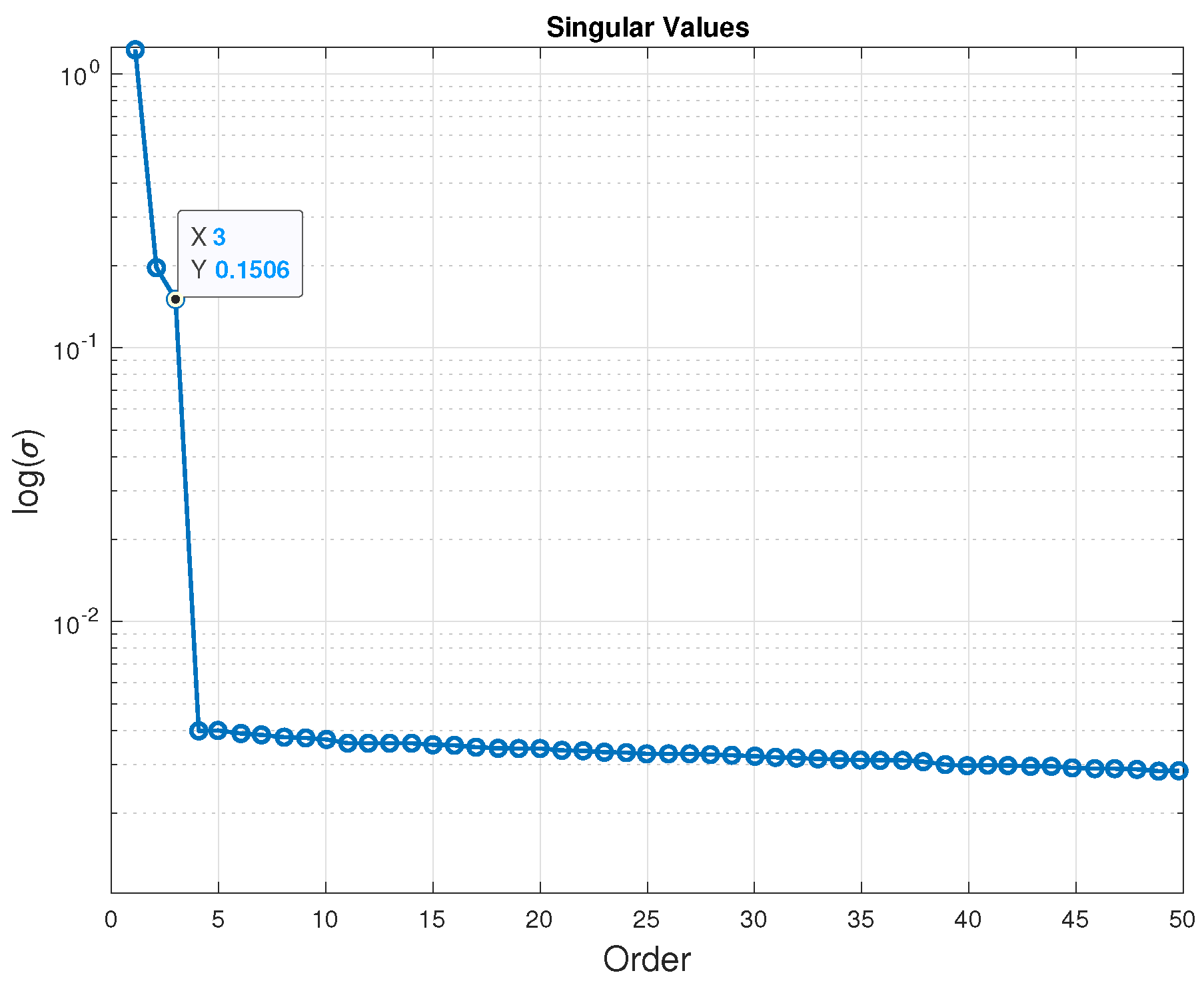
The identification process is repeated for a case where white noise is added to the LTI input–output data. The white noise has a signal-to-noise ratio of 20 when applied to the output data. The singular values for this case are shown in Figure 5. As for the case without noise, a gap is still clearly seen between the third and fourth singular values of the identified dynamics. As such, the order of the identified model is chosen to be three and its eigenvalues are shown in Figure 6.

4.2. Harmonic Analyzer’s Effect on the Identification

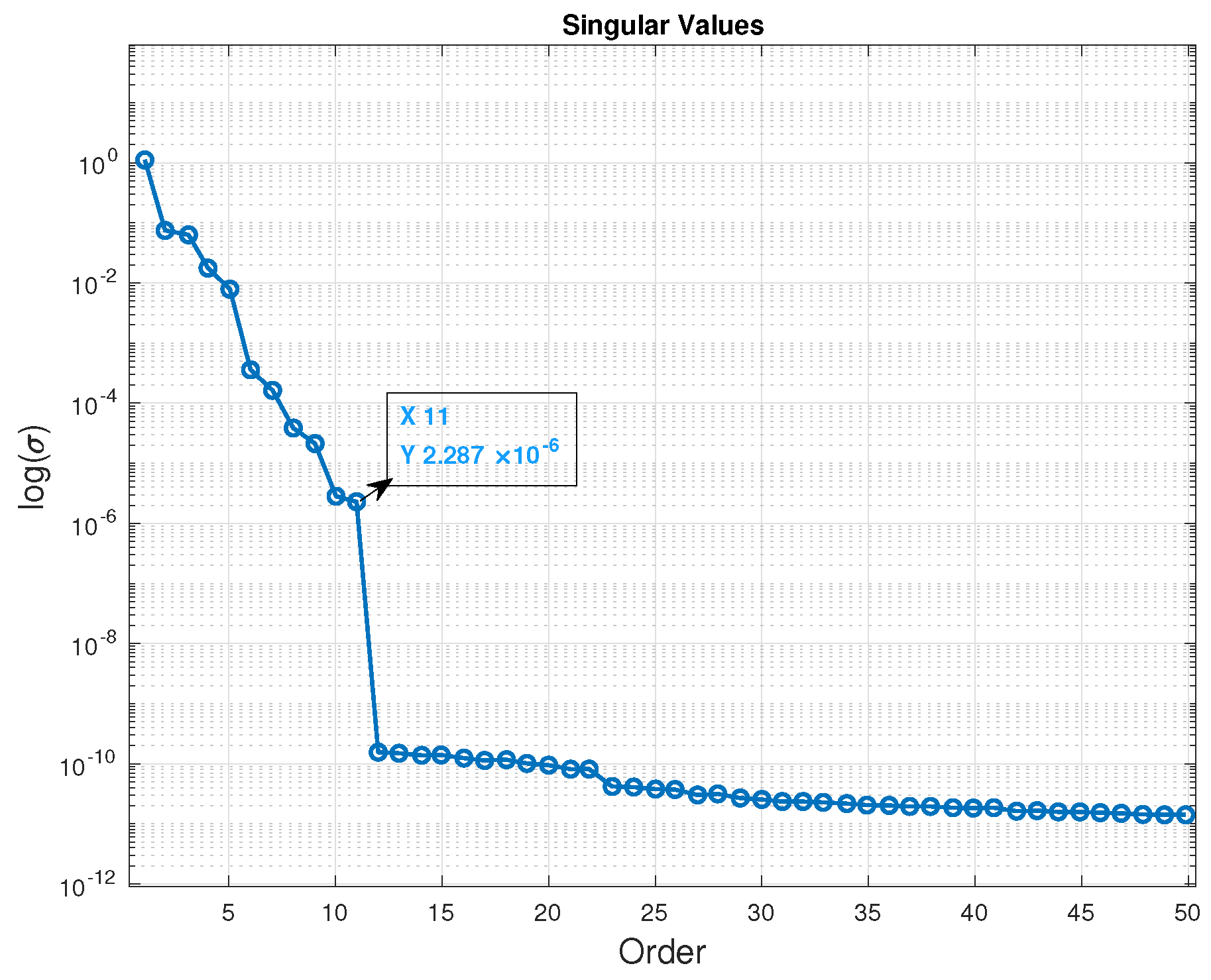
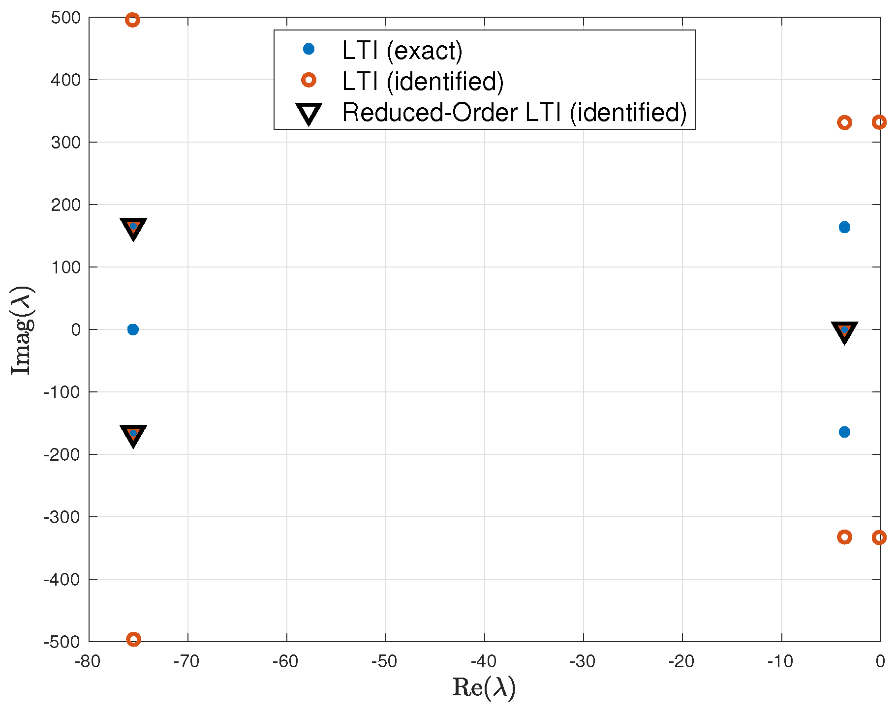
Because input–output data from either the LTP or NLTP dynamics are not readily available in the harmonic components, a harmonic analyzer must be used to compute the harmonics of the output signals. However, the harmonic analyzer may introduce distortions in the signal that may hinder the identification process. In this section, the effect of the harmonic analyzer on the identification process is assessed. To carry out this assessment, the perturbation response corresponding to the LTP system states is first reconstructed from the LTI input–output data using Equation (7c). Then, the harmonic coefficients are extracted from the perturbation response using the harmonic analyzer. When these data are used in the identification process, the jump in the singular values occurs at the eleventh singular value rather than at the third, as shown in Figure 7. This indicates that the harmonic analyzer introduced spurious dynamics in the identified model. These are high-frequency dynamics introduced by the windowing effect of the harmonic analyzer. The eigenvalues of the identified 11-state system are shown in Figure 8. In spite of the introduction of high-frequency dynamics and thus extra eigenvalues, the three eigenvalues corresponding to the heave dynamics subsystem are identified correctly. Model order reduction is then used to retain only those three states associated with the heave dynamics, which are shown against the eigenvalues of the known dynamics in Figure 8.

4.2.1. Identification from LTP Input-Output Data

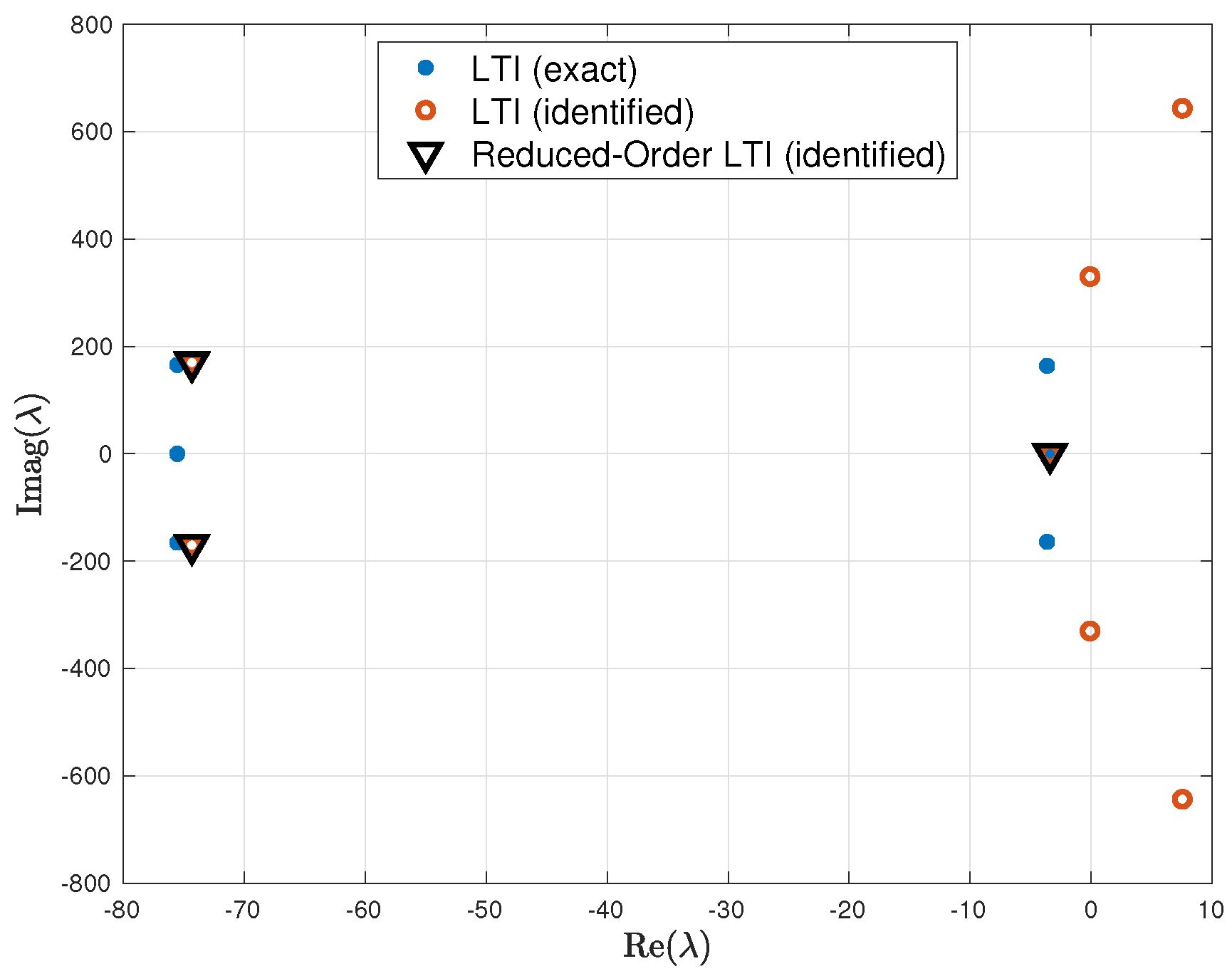
Once the effect of the harmonic analyzer is understood, it can be applied to identify the high-order LTI dynamics from LTP data. The LTP data are generated by feeding the same doublet input used for the LTI dynamics into the LTP system, and by measuring the perturbation response in the vertical speed and flapping angle. The LTP system;s response is shown in Figure 2 with a blue line. Then, the harmonic analyzer is applied to the output data to extract the signals $w_0$, ${\dot{\varphi }}_{1c}$, and ${\dot{\varphi }}_{1s}$. The singular values of the identified dynamics are shown in Figure 9. A gap is observed between the seventh and eighth singular values. As such, the order of the system is selected to be seven. The eigenvalues of the identified seven-state system are shown in Figure 10. Again, while high-frequency eigenvalues are introduced by the harmonic analyzer, the three eigenvalues corresponding to the heave dynamics subsystem appear to be identified correctly. The spurious high-frequency dynamics is truncated and residualized and the three-state model eigenvalues are shown in Figure 10.

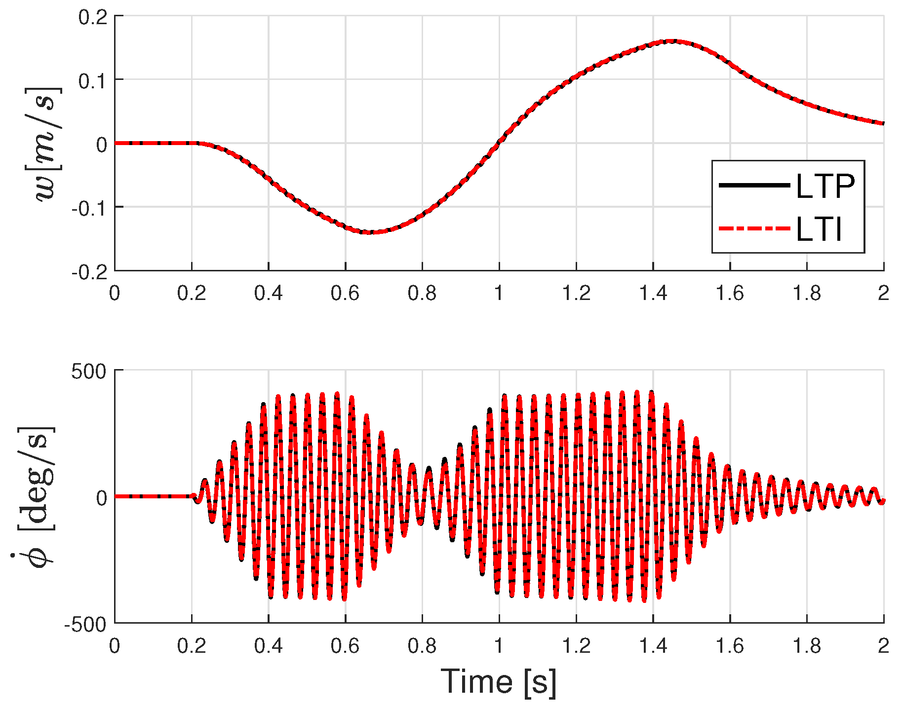
To validate the identified three-state dynamics in the time domain, the responses of the identified dynamics and LTP dynamics are compared for a double input different to that used in the identification process. The responses are shown in Figure 11, where the output of the identified system nearly overlaps with that of the LTP system. Note that Equation (7c) was used to reconstruct the perturbation response from the LTI system’s output. These results suggest the suitability of the proposed approach for the identification of high-order LTI dynamics from LTP system responses when applied to simple FWMAV models.

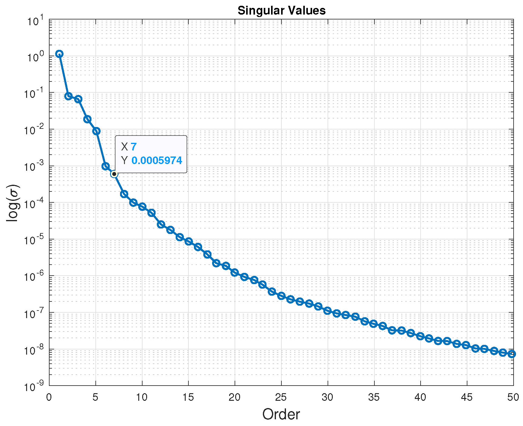
The process is repeated for the case where white noise is applied to the input–output data prior to the use of the harmonic analyzer. The signal-to-noise ratio is again chosen to be 20. The singular values plot from the identification is shown in Figure 12. When compared to Figure 9, a clearer jump is noted after the seventh singular value. Nonetheless, the harmonic analyzer introduces four extra eigenvalues into the identification. Once again, in spite of the four extra eigenvalues, the three eigenvalues corresponding to the heave dynamics are correctly identified. The eigenvalues after the application of model-order reduction to remove the spurious dynamics are shown in Figure 13 and correspond to those of the original vertical-motion dynamics subsystem.

4.2.2. Identification from NLTP Input–Output Data

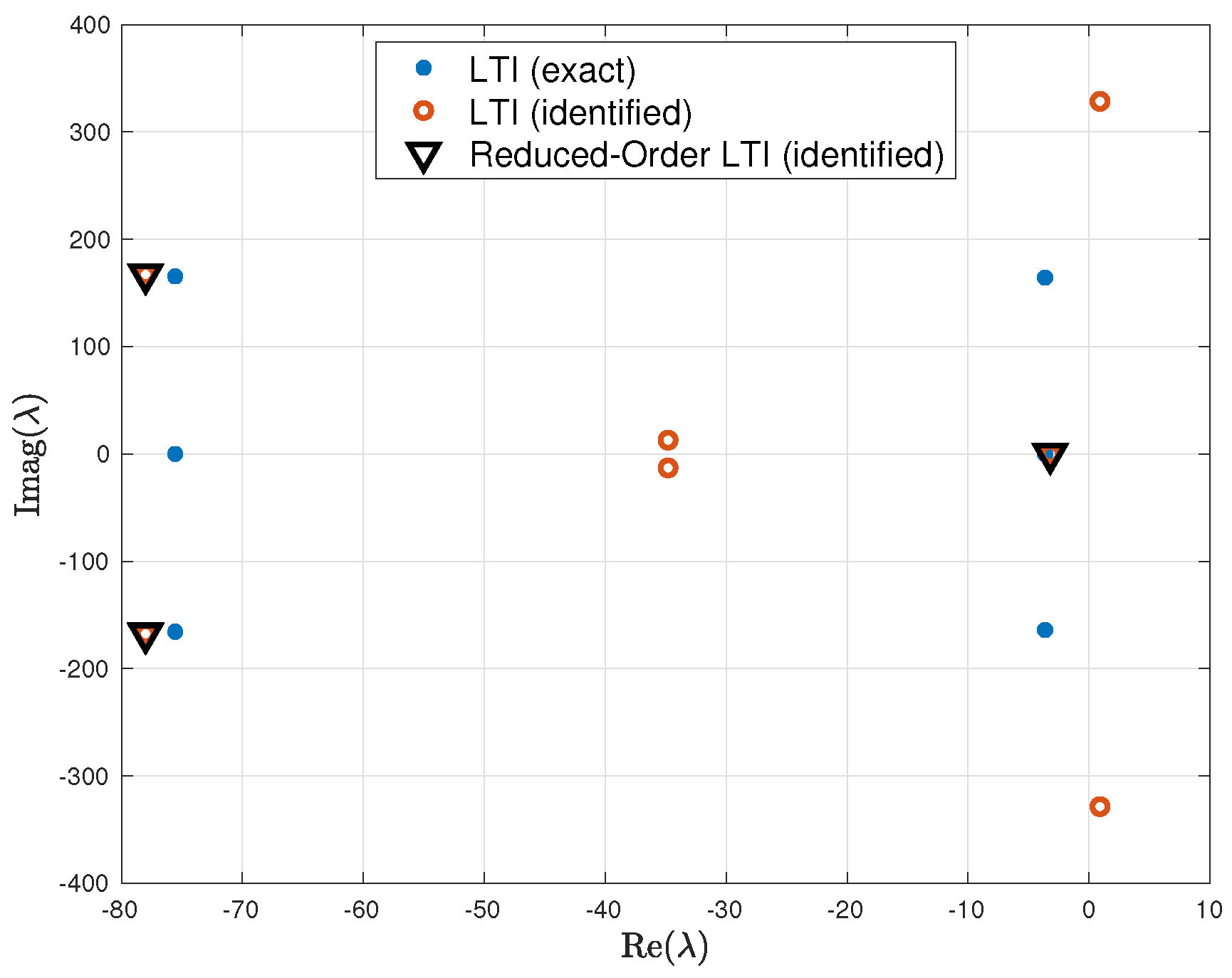
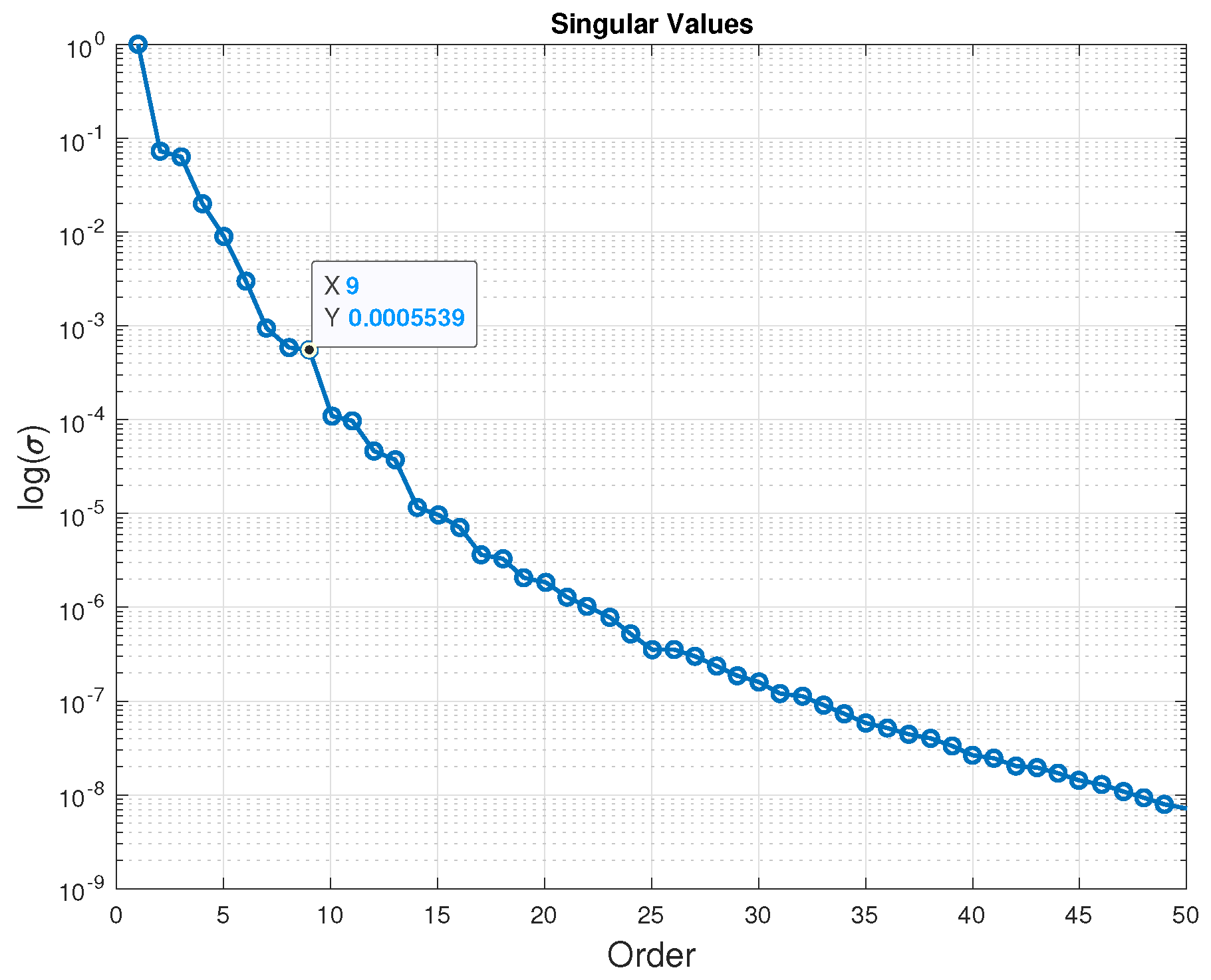
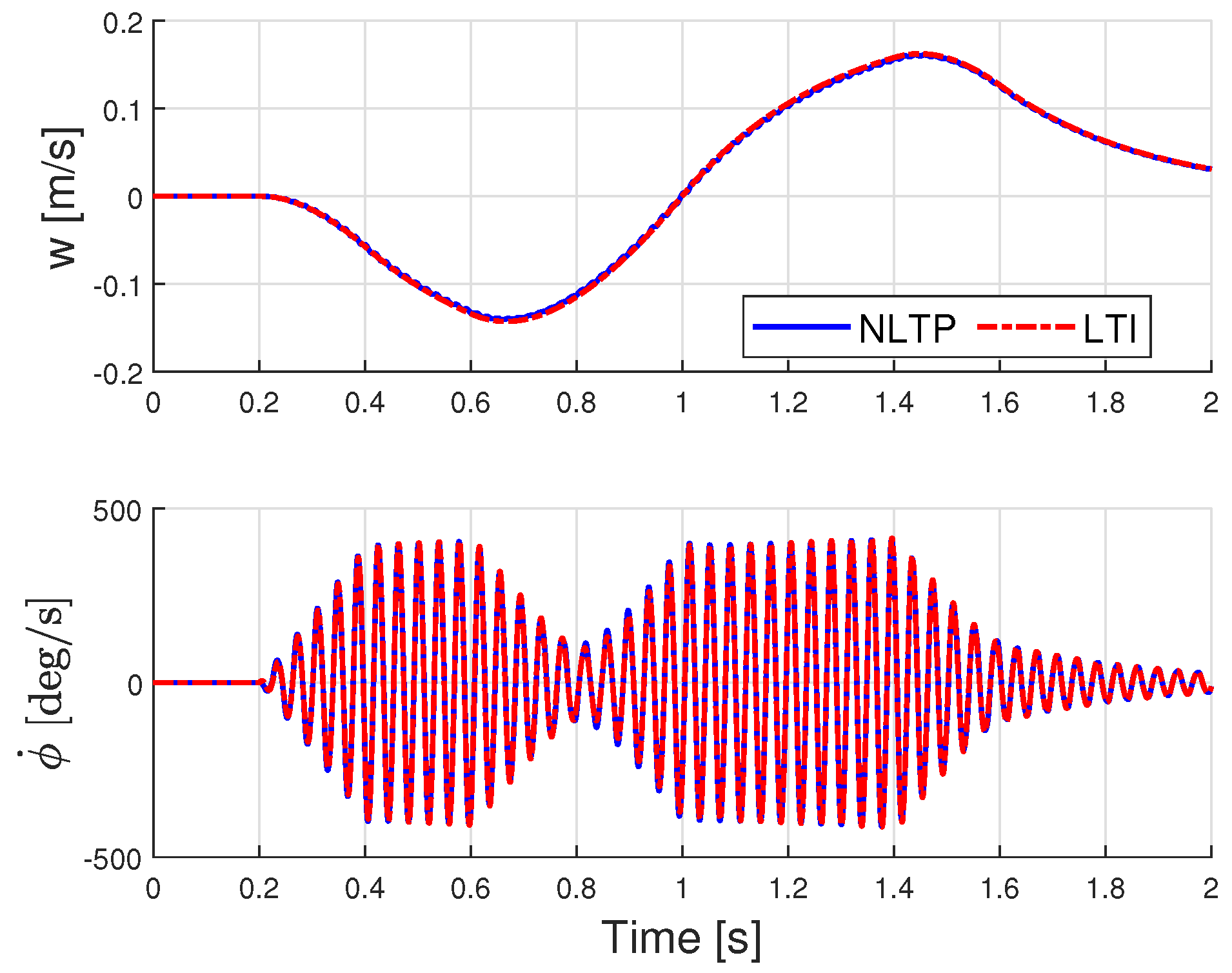
As a last example, the identification process has been performed based on input–output data obtained from the NLTP dynamics. After obtaining the NLTP system response using the same control input doublet used in the previous examples, the periodic trim solution is subtracted from the input–output data to find the control input and state perturbations. The resulting signals are processed with the harmonic analyzer to decompose the signal into harmonics of the fundamental frequency of the system. The Fourier coefficients of the input-output data are then used in the identification process. The singular values resulting from the subspace identification are shown in Figure 14. In this figure, a clear jump is seen at the ninth singular value, indicating that once again the harmonic analyzer introduces spurious dynamics. The eigenvalues of the identified nine-state system as well as the reduced-order model eigenvalues are shown in Figure 15. The eigenvalues of the reduced-order model are very similar to those of the known system. To validate the identified three-state dynamics in the time domain, responses of the identified dynamics and NLTP dynamics are compared for a doublet input different than that used in the identification process. The responses are shown in Figure 16, where the output of the identified system nearly overlaps that of the NLTP system. These results suggest the suitability of the proposed approach also for the identification of the high-order LTI approximate dynamics from NLTP system responses, when applied to simple FWMAV models.

4.3. Model Matching

Model matching is performed by leveraging the robust control toolbox in MATLAB^® R2020a. It is assumed that the outputs correspond to the states in harmonic decomposition form and that the feedthrough matrix is equal to zero (i.e., $\mathit{D}=\mathbf{0}$). The unstructured matrices identified with subspace identification are converted to continuous-time form using the d2c function. Next, the continuous-time state–space model thus obtained is compared to the parametrized state–space model using the function hinfstruct. This command solves for those unknown parameters $\mathit{\theta }$ of the structured system that minimize the $H_{\infty }$ norm of the difference between the identified dynamics and the structured system. In the minimization process, the $H_{\infty }$ norm tolerance is set to $1\times {10}^{-20}$, and the target gain is set to $1\times {10}^{-3}$. The minimization problem is run for all of the examples presented above. The system matrix $\mathit{A}$ for each case is found and compared to the original upper left $3\times 3$ matrix from Equation (26). The Frobenius norm is used to find the percentage error between the identified and known structured system matrices. Table 1 shows the percentage error in the difference between the exact and the identified matrices for all of these cases above, where the error is defined as

$$e={\displaystyle \frac{|\mathit{A}\left({\mathit{\theta }}^{\ast }\right)-{\mathit{A}}_{\mathrm{exact}}{|}_F}{|{\mathit{A}}_{\mathrm{exact}}{|}_F}}$$

(27)

The dynamics identified from the LTI input–output data provide the best match with the exact dynamics. In fact, the match is almost perfect. This does not come as a surprise as this is also the case when the harmonic analyzer is assumed to be perfect. The remaining cases show that the use of the harmonic analyzer reduces the accuracy of the identified dynamics, and that identification using NLTP dynamics is less precise than that using LTP data.

Table 1. Percentage error of the difference between the identified structured system matrix and the exact dynamics in harmonic decomposition form.

Input-Output Data Type	Error, e [%]
LTI	9.0843$\times {10}^{-7}$
LTI + Noise	0.0767
LTI + Harmonic Analyzer	0.0026
LTP	0.328
LTP + Noise	0.4514
NLTP data	4.1337

Table 1. Percentage error of the difference between the identified structured system matrix and the exact dynamics in harmonic decomposition form.

Input-Output Data Type	Error, e [%]
LTI	9.0843$\times {10}^{-7}$
LTI + Noise	0.0767
LTI + Harmonic Analyzer	0.0026
LTP	0.328
LTP + Noise	0.4514
NLTP data	4.1337

5. Conclusions

In this work, the use of subspace identification was extended toward the direct identification of higher-order LTI systems in harmonic decomposition form from nonlinear time-periodic system (NLTP) responses. The methodology was demonstrated through examples involving the NLTP dynamics of a flapping-wing micro aerial vehicle (FWMAV). Examples focused on the identification of the heave dynamics from various types of input–output data, including LTI, LTP, and NLTP input–output data. The effect of a harmonic analyzer to decompose the LTP and NLTP responses into harmonics was assessed on the identification process. The effect of white noise on the identification process was studied as well. Based on this work, the following conclusions can be reached.

• The application of harmonic analyzers to decompose input–output data into harmonics of the fundamental frequency of the system introduces spurious dynamics into the identified system. These spurious dynamics make it challenging to determine the correct order of the system. When the order of the system is known, these spurious dynamics can be removed using model order reduction methods such as truncation and residualization. However, some prior knowledge of the system is necessary to remove the spurious dynamics introduced by the harmonic analyzer.
• The mismatch between the identified and exact systems when the identification is performed from LTI input–output data (i.e., for the case where the harmonic analyzer is perfect) is very small. The mismatch grows, but is still acceptable, if the identification is performed using harmonically decomposed LTP and NLTP input–output data.
• Noise is shown to have a negative effect on the accuracy of the identification. Additionally, noise makes it harder to determine the true order of the system.
• Model matching us allowed to recover the harmonic decomposition structure in the identified model. However, previous knowledge of the system to be identified is necessary for this step. This prior knowledge is essential to distinguish genuine system dynamics from spurious dynamics introduced by the harmonic analyzer and the identification process.

The methodology can be applied to more complex and higher-order systems such as the longitudinal flight dynamics of FWMAVs, to helicopter rotors, and to rotorcraft in general. An important consideration in this methodology, however, is the requirement of prior knowledge of the physics during the model matching phase. Such prior knowledge is crucial to differentiate the system’s behavior from artificial dynamics that result from the harmonic analysis and identification methods. Without this understanding, it becomes challenging to accurately determine the true order of the system and to remove irrelevant dynamics effectively. Furthermore, transitioning from the identified LTI models back to the original LTP models is not easy due to the complexities inherent in NLTP systems. Therefore, while this approach can successfully identify LTI models that are directly usable for analysis and design control, it does not directly produce the corresponding LTP models. Future work could incorporate the application of this identification technique to systems with time-varying delays like those in Refs. [41,42].

References

1. Friedmann, P.P.; Millott, T.A. Vibration reduction in rotorcraft using active control—A comparison of various approaches. J. Guid. Control Dyn. 1995, 18, 664–673. [Google Scholar] [CrossRef]
2. Abraham, M.D.; Olcer, F.E.; Costello, M.F.; Takahashi, M.D.; Tischler, M.D. Integrated Design of AFCS and HHC for Rotorcraft Vibration Reduction using Dynamic Crossfeed. In Proceedings of the 67th Annual Forum of the American Helicopter Society, Virginia Beach, VA, USA, 3–5 May 2011. [Google Scholar]
3. Padthe, A.K.; Friedmann, P.P.; Lopez, M.; Prasad, J.V.R. Analysis of High Fidelity Reduced-Order Linearized Time-Invariant Helicopter Models for Integrated Flight and On-Blade Control Applications. In Proceedings of the 41st European Rotorcraft Forum, Munich, Germany, 1–4 September 2015. [Google Scholar]
4. Lopez, M.; Prasad, J.V.R.; Tischler, M.B.; Takahashi, M.D.C.K.K. Simulating HHC/AFCS Interaction and Optimized Controllers using Piloted Maneuvers. In Proceedings of the 71st Annual Forum of the American Helicopter Society, Virginia Beach, VA, USA, 5–7 May 2015. [Google Scholar]
5. Lopez, M.; Tischler, M.; Takahashi, M.; Cheung, K.; Prasad, J. Development and Evaluation of a Full Flight Envelope Integrated Flight and Vibration Controller. J. Am. Helicopter Soc. 2018, 64, 1–11. [Google Scholar] [CrossRef]
6. Saetti, U.; Horn, J.F. Load Alleviation Flight Control Design using High-Order Dynamic Models. J. Am. Helicopter Soc. 2020, 65, 1–15. [Google Scholar] [CrossRef]
7. Saetti, U.; Horn, J.F.; Berger, T.; Tischler, M.B. Handling-Qualities Perspective on Rotorcraft Load Alleviation Control. J. Guid. Control Dyn. 2020, 43, 1792–1804. [Google Scholar] [CrossRef]
8. Saetti, U.; Lovera, M. Time-Periodic and High-Order Time-Invariant Linearized Models of Rotorcraft: A Survey. J. Am. Helicopter Soc. 2022, 67, 1–19. [Google Scholar] [CrossRef]
9. Sanders, J.A.; Verhulst, F.; Murdock, J. Averaging Methods in Nonlinear Dynamical Systems; Chapter Averaging: The periodic case; Springer: Berlin/Heidelberg, Germany, 2007. [Google Scholar]
10. Hassan, A.M.; Taha, H.E. Higher-Order Averaging Analysis of the Nonlinear Time-Periodic Dynamics of Hovering Insects/ Flapping-Wing Micro-Air-Vehicles. In Proceedings of the 55th Conference on Decision and Control, Las Vegas, NV, USA, 12–14 December 2016. [Google Scholar] [CrossRef]
11. Maggia, M.; Eisa, S.A.; Taha, H.E. On higher-order averaging of time-periodic systems: Reconciliation of two averaging techniques. Nonlinear Dyn. 2020, 99, 813–836. [Google Scholar] [CrossRef]
12. Floquet, G. Sur les équations différentielles linéaires à coefficients périodiques. Ann. Sci. De L’École Norm. Supérieure 1883, 2, 47–88. [Google Scholar] [CrossRef]
13. Dietl, J.M.; Garcia, E. Stability in Ornithopter Longitudinal Flight Dynamics. J. Guid. Control Dyn. 2008, 31, 1157–1163. [Google Scholar] [CrossRef]
14. Bierling, T.; Patil, M. Stability and Power Optimality in Time-Periodic Flapping Wing Structures. J. Fluids Struct. 2013, 38, 238–254. [Google Scholar] [CrossRef]
15. Su, W.; Cesnik, C.E.S. Flight Dynamic Stability of a Flapping Wing Micro Air Vehicle in Hover. In Proceedings of the 52nd AIAA/ASME/ASCE/AHS/ACS Structures, Structural Dynamics, and Materials Conference, Denver, CO, USA, 4–7 April 2011. [Google Scholar] [CrossRef]
16. Lopez, M.J.S.; Prasad, J.V.R. Linear Time Invariant Approximations of Linear Time Periodic Systems. J. Am. Helicopter Soc. 2017, 62, 1–10. [Google Scholar] [CrossRef]
17. Saetti, U.; Rogers, J.D. Revisited Harmonic Balance Trim Solution Method for Periodically-Forced Aerospace Vehicles. J. Guid. Control Dyn. 2021, 44, 1008–1017. [Google Scholar] [CrossRef]
18. Passaro, M.; Lovera, M. LPV model identification of a flapping wing MAV. In Proceedings of the 4th IFAC Workshop on Linear Parameter Varying Systems, Milan, Italy, 19–20 July 2021; pp. 27–32. [Google Scholar] [CrossRef]
19. Armanini, S.F.; de Visser, C.C.; de Croon, H.E.; Mulder, M. Time-Varying Model Identification of Flapping-Wing Vehicle Dynamics Using Flight Data. J. Guid. Control Dyn. 2015, 139, 526–541. [Google Scholar] [CrossRef]
20. Gim, H.; Kim, S.; Suk, J.; Cho, S. Longitudinal System Identification of Ornithopter with Automated Flight Tests. In Proceedings of the 20th IFAC Symposium on Automatic Control in Aerospace, Sherbrooke, QC, Canada, 19–20 July 2016; pp. 27–32. [Google Scholar] [CrossRef]
21. Hench, J. A technique for the identification of linear periodic state space models. Int. J. Control 1995, 62, 289–301. [Google Scholar] [CrossRef]
22. Verhaegen, M.; Yu, X. A class of subspace model identification algorithms to identify periodically and arbitrarily time-varying systems. Automatica 1995, 31, 201–261. [Google Scholar] [CrossRef]
23. Van Overschee, P.; De Moor, B. Subspace Identification for Linear Systems. Theory, Implementation, Applications; Springer Science & Business Media: New York, NY, USA, 1996. [Google Scholar]
24. Liu, K. Identification of linear time-varying systems. J. Sound Vib. 1997, 206, 487–505. [Google Scholar] [CrossRef]
25. Felici, F.; van Wingerden, J.; Verhaegen, M. Subspace identification of MIMO LPV systems using a periodic scheduling sequence. Automatica 2007, 43, 1684–1697. [Google Scholar] [CrossRef]
26. Yin, W.; Mehr, A. Identification of linear periodically time-varying systems using periodic sequences. In Proceedings of the 2009 IEEE International Conference on Control Applications, Petersburg, Russia, 8–10 July 2009. [Google Scholar] [CrossRef]
27. Louarroudi, E.; Pintelon, R.; Lataire, J. Nonparametric tracking of the time-varying dynamics of weakly nonlinear periodically time-varying systems using periodic inputs. IEEE Trans. Instrum. Meas. 2012, 61, 1384–1394. [Google Scholar] [CrossRef]
28. Goos, J.; Pintelon, R. Continuous-time identification of periodically parameter-varying state space models. Automatica 2016, 71, 254–263. [Google Scholar] [CrossRef]
29. Wood, T.A. Model-Based Flight Control of Kites for Wind Power Generation. Ph.D. Thesis, ETH Zurich, Zurich, Switzerland, 2011. [Google Scholar]
30. Uyanik, I.; Saranli, U.; Ankarali, M.; Cowan, N.; Morgul, O. Frequency-domain subspace identification of linear time-periodic (LTP) systems. IEEE Trans. Autom. Control 2019, 64, 2529–2536. [Google Scholar] [CrossRef]
31. Yin, M.; Iannelli, A.; Khosravi, M.; Parsi, A.; Smith, R.S. Linear Time-Periodic System Identification with Grouped Atomic Norm Regularization. In Proceedings of the 21st IFAC World Congress, Berlin, Germany, 11–17 July 2020; pp. 1237–1242. [Google Scholar] [CrossRef]
32. Hayajnh, M.; Saetti, U.; Prasad, J. Identification of High-Order Linear Time-Invariant Models from Periodic Nonlinear System Responses. In Proceedings of the VFS 9th Annual ElectricVTOL Symposium, San Jose, CA, USA, 25–27 January 2022. [Google Scholar]
33. Van Overschee, P.; De Moor, B. Continuous-time frequency domain subspace system identification. Signal Process. 1996, 52, 179–194. [Google Scholar] [CrossRef]
34. Verhaegen, M.; Dewilde, P. Subspace model identification part 1. The output-error state-space model identification class of algorithms. Int. J. Control 1992, 56, 1187–1210. [Google Scholar] [CrossRef]
35. Van Overschee, P.; De Moor, B. A unifying theorem for three subspace system identification algorithms. Automatica 1995, 31, 1853–1864. [Google Scholar] [CrossRef]
36. Kokotovic, P.; O’Malley, R.; Sannuti, P. Singular perturbations and order reduction in control theory—An overview. Automatica 1976, 12, 123–132. [Google Scholar] [CrossRef]
37. Bergamasco, M.; Lovera, M. State space model identification: From unstructured to structured models with an H approach. IFAC Proc. Vol. 2013, 46, 202–207. [Google Scholar] [CrossRef]
38. Gahinet, P.; Apkarian, P. Decentralized and fixed-structure H control in MATLAB. In Proceedings of the 2011 50th IEEE Conference on Decision and Control and European Control Conference, Orlando, FL, USA, 12–15 December 2011; pp. 8205–8210. [Google Scholar] [CrossRef]
39. Saetti, U.; Rogers, J.D. Harmonic Decomposition Models of Flapping-Wing Flight for Stability Analysis and Control Design. J. Guid. Control. Dyn. 2022, 45, 8. [Google Scholar] [CrossRef]
40. Lopez, M.J.S.; Prasad, J.V.R. Estimation of Modal Participation Factors of Linear Time Periodic Systems Using Linear Time Invariant Approximations. J. Am. Helicopter Soc. 2016, 61, 1–4. [Google Scholar] [CrossRef]
41. Hernández-González, B.O.; Targui, G.V.P.; Guerrero-Sánchez, M. Robust cascade observer for a disturbance unmanned aerial vehicle carrying a load under multiple time-varying delays and uncertainties. Int. J. Syst. Sci. 2024, 55, 1056–1072. [Google Scholar] [CrossRef]
42. Hernández-González, O.; Ramírez-Rasgado, F.; Farza, M.; Guerrero-Sánchez, M.E.; Astorga-Zaragoza, C.M.; M’Saad, M.; Valencia-Palomo, G. Observer for Nonlinear Systems with Time-Varying Delays: Application to a Two-Degrees-of-Freedom Helicopter. Aerospace 2024, 11, 206. [Google Scholar] [CrossRef]
Figure 1. Modal participation factors for the vertical dynamics of the FWMAV in hover. (a) Vertical speed; (b) flapping speed.
Aerospace 11 00875 g001
Figure 2. Response of the NLTP, LTP and high-order LTI vertical dynamics of a FWMAV to a doublet input in the flapping torque.
Aerospace 11 00875 g002
Figure 3. Singular values when using LTI input-output data directly (no noise).
Aerospace 11 00875 g003
Figure 4. Identified vs. true eigenvalues using LTI input–output data directly (no noise).
Aerospace 11 00875 g004
Figure 5. Singular values when using LTI input-output data directly (with noise).
Aerospace 11 00875 g005
Figure 6. Identified vs. true eigenvalues using LTI input–output data directly (with noise).
Aerospace 11 00875 g006
Figure 7. Harmonic analyzer’s effect on the singular values.
Aerospace 11 00875 g007
Figure 8. Identified vs. true eigenvalues when using the harmonic analyzer.
Aerospace 11 00875 g008
Figure 9. Singular values when using LTP input–output data (no noise).
Aerospace 11 00875 g009
Figure 10. Identified vs. true eigenvalues using LTP input–output data (no noise).
Aerospace 11 00875 g010
Figure 11. Identified LTI vs. original LTP responses following a control input doublet.
Aerospace 11 00875 g011
Figure 12. Singular values when using LTP input-output data (with noise).
Aerospace 11 00875 g012
Figure 13. Comparison between the identified and original systems’ eigenvalues when using the harmonic analyzer on the LTP signals with measurement noise.
Aerospace 11 00875 g013
Figure 14. Singular values when using NLTP input–output data (no noise).
Aerospace 11 00875 g014
Figure 15. Identified vs. true eigenvalues using NLTP input–output data (no noise).
Aerospace 11 00875 g015
Figure 16. Identified LTI vs. original NLTP responses following a control input doublet.
Aerospace 11 00875 g016
Disclaimer/Publisher’s Note: The statements, opinions and data contained in all publications are solely those of the individual author(s) and contributor(s) and not of MDPI and/or the editor(s). MDPI and/or the editor(s) disclaim responsibility for any injury to people or property resulting from any ideas, methods, instructions or products referred to in the content.