
Measurement of Driving Conditions of Aircraft Ground Support Equipment at Tokyo International Airport


Abstract
1. Introduction
2. Literature Review
3. Methodology
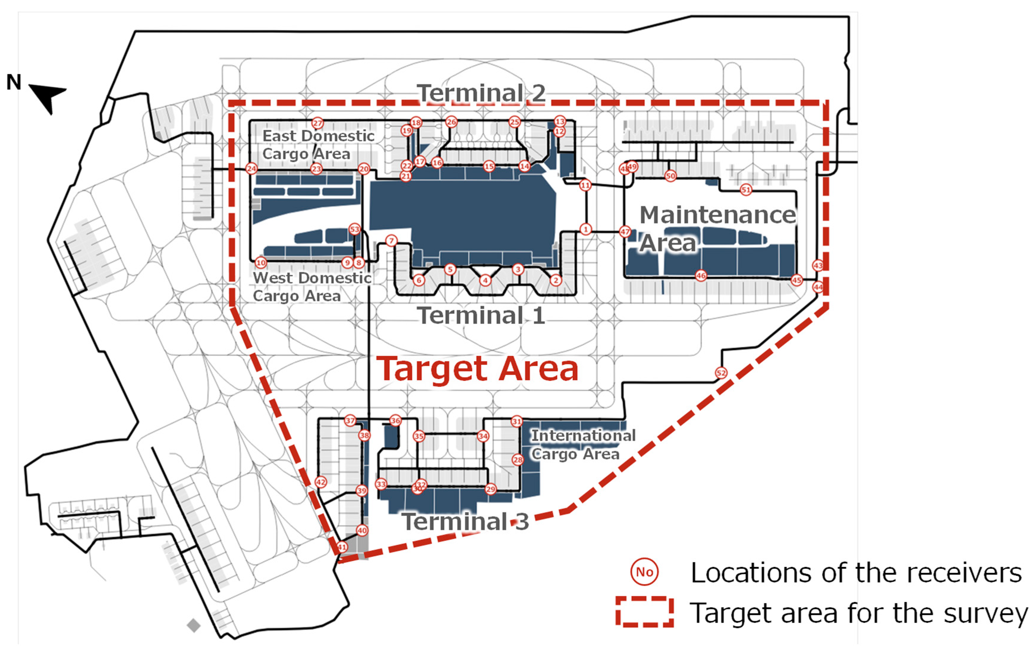
3.1. Survey Scope and Data Collection
3.2. Trip Data Creation Method
3.2.1. Extraction of Target Trips
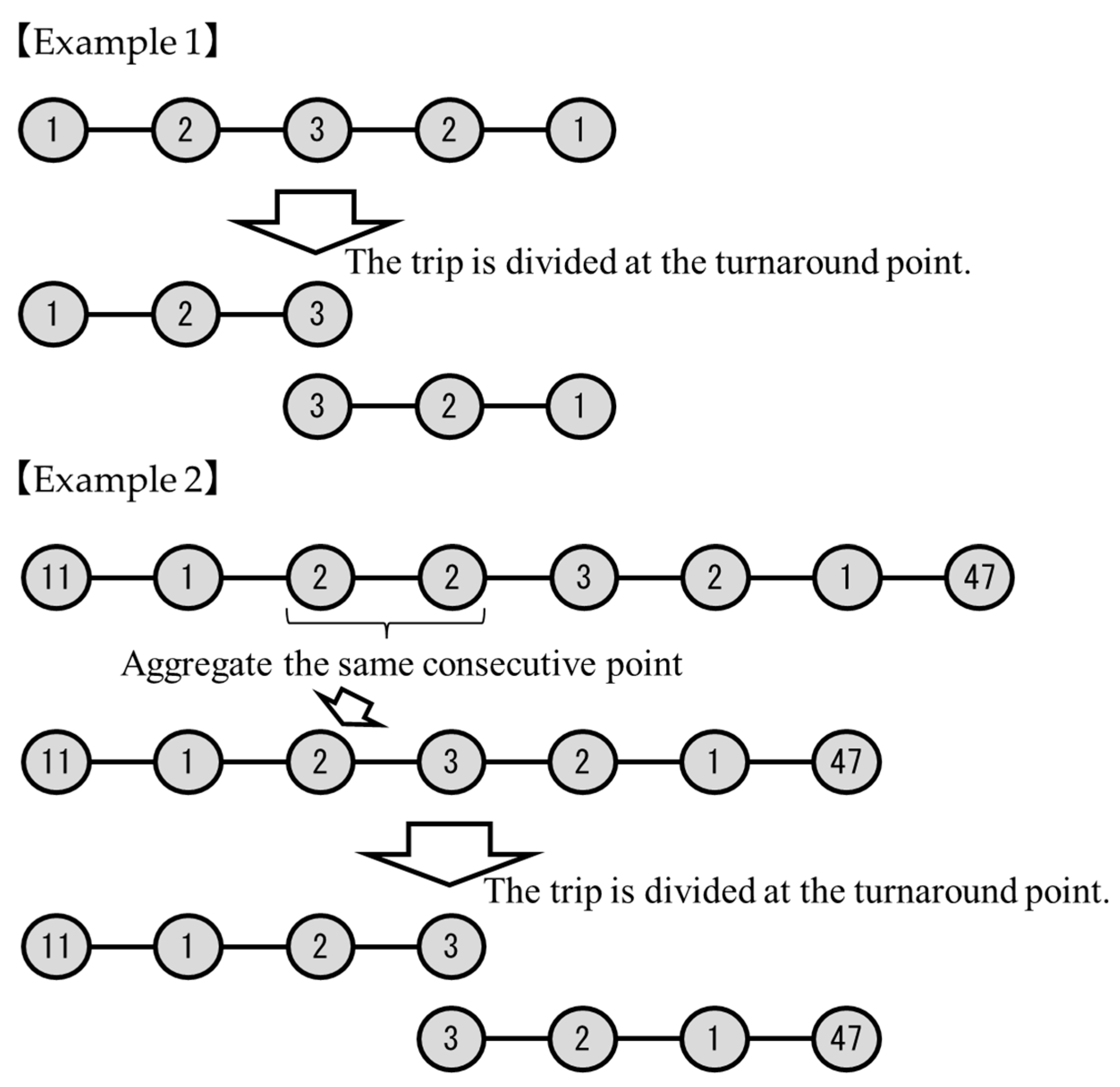
3.2.2. Turnaround Trips
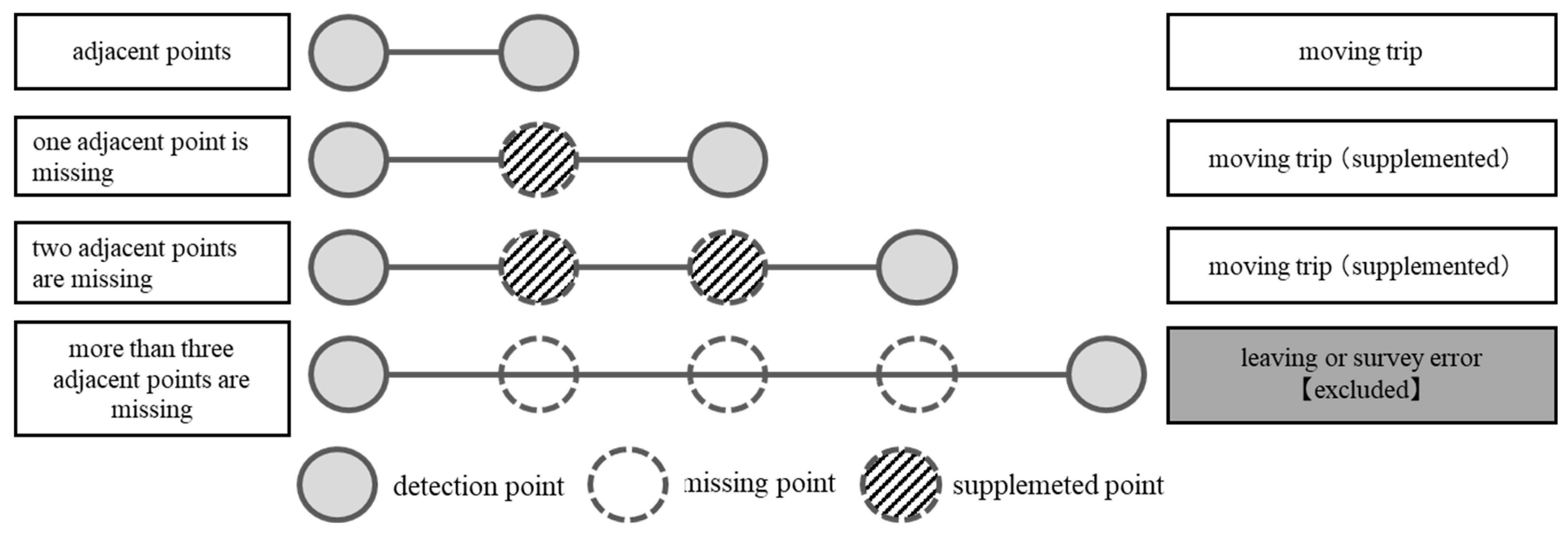
3.2.3. Expansion Estimates of Moving Trips
4. Results
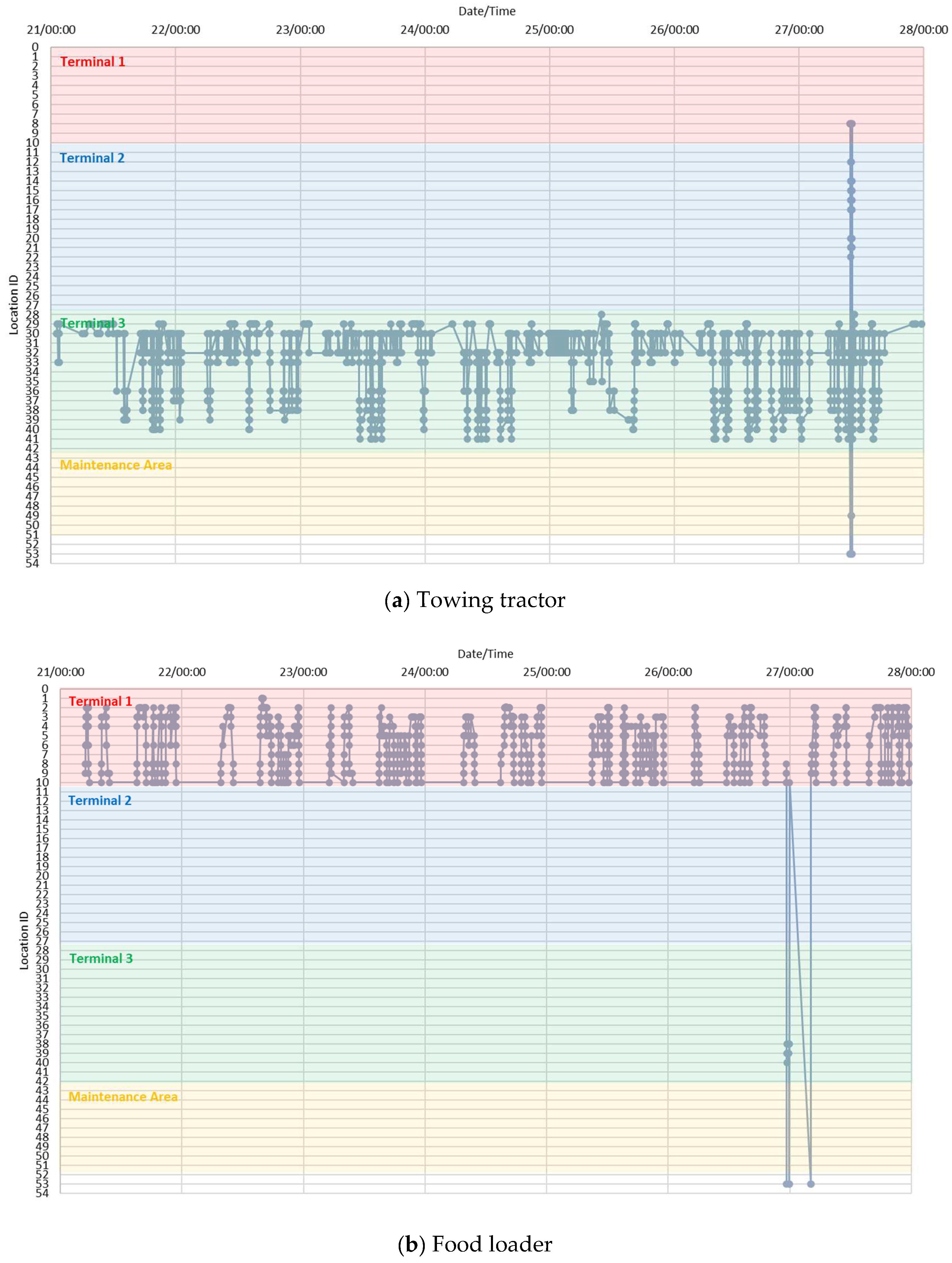
4.1. Results of the Detection Record Data
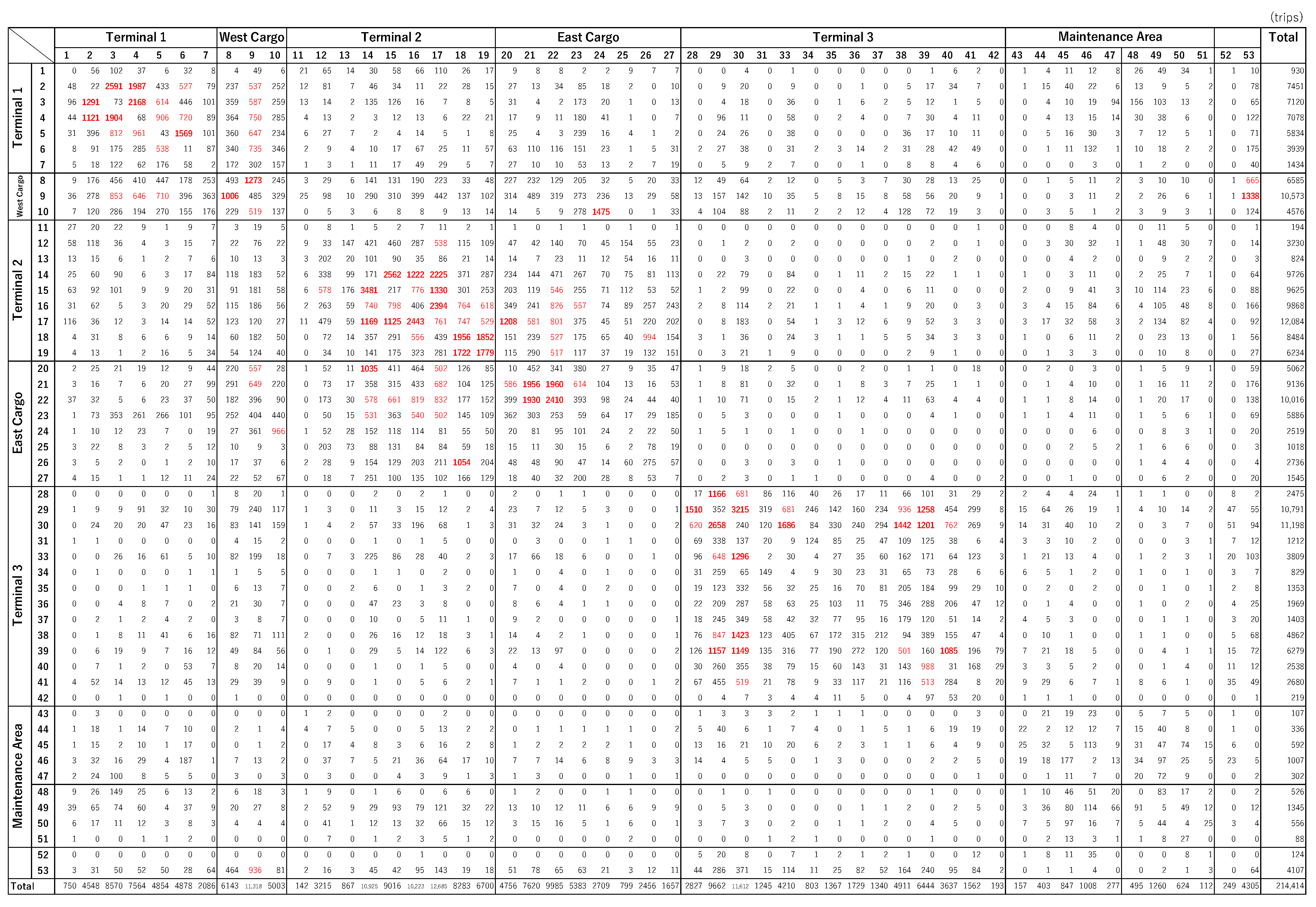
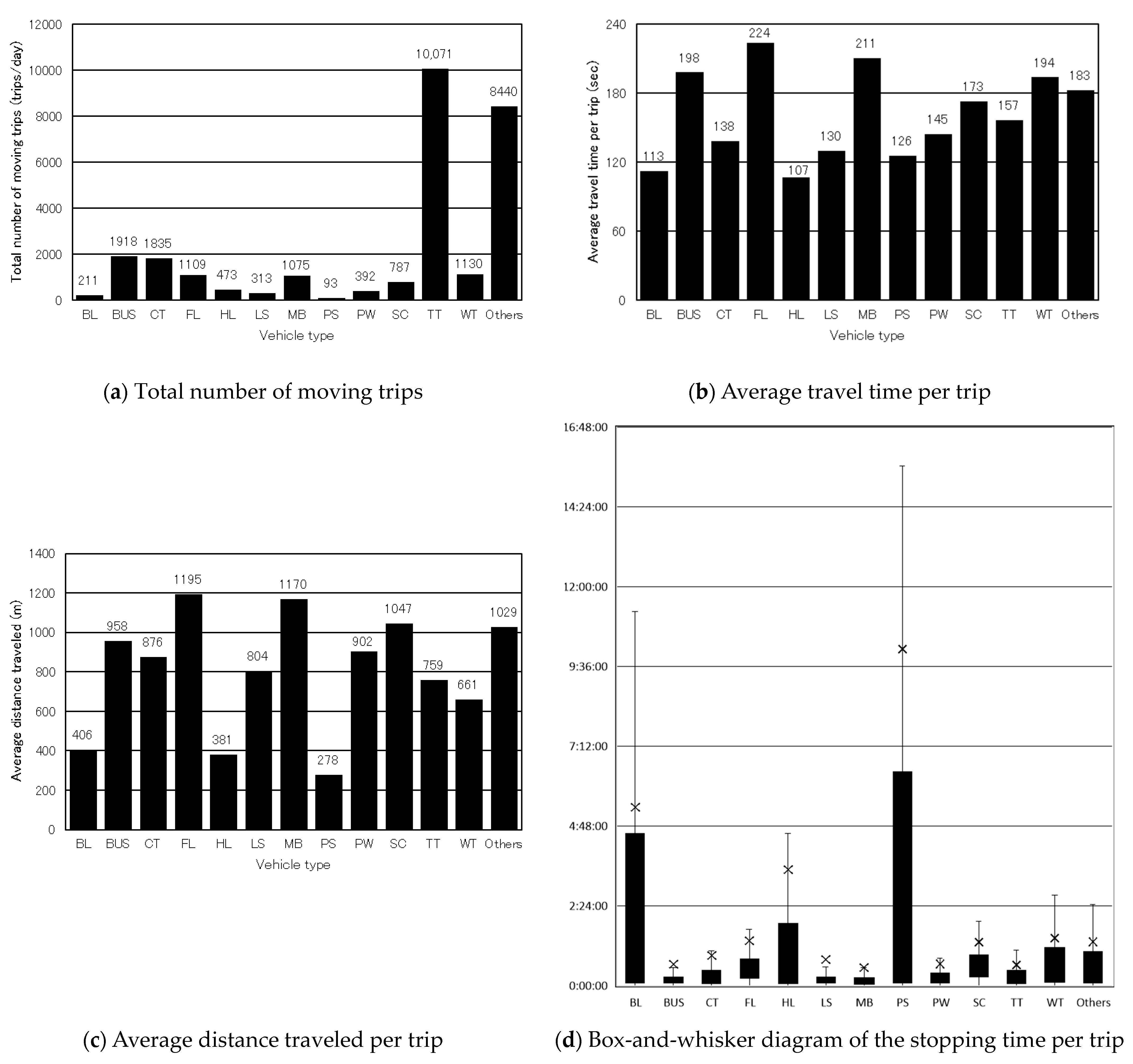
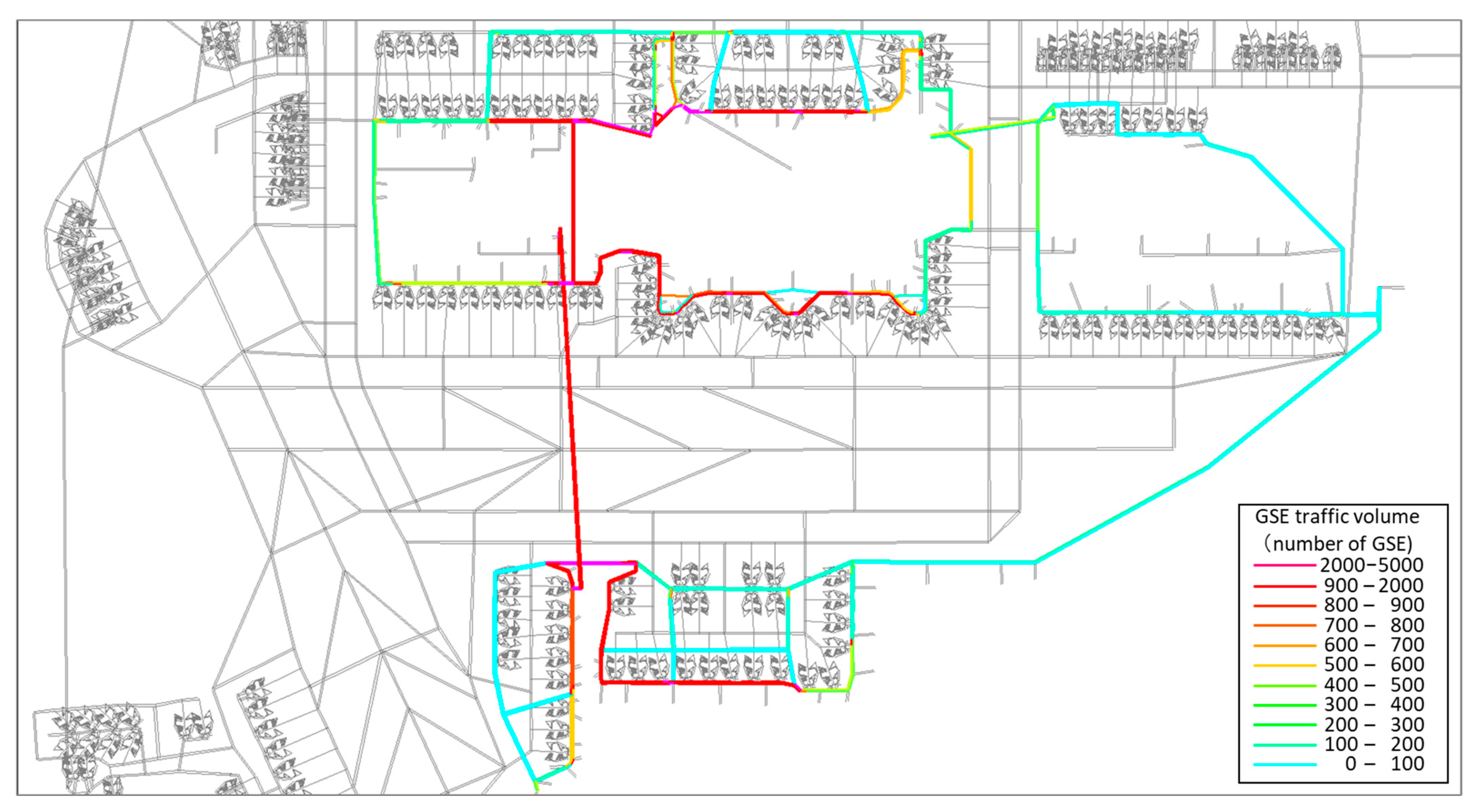
4.2. Results of Trip Data Organization
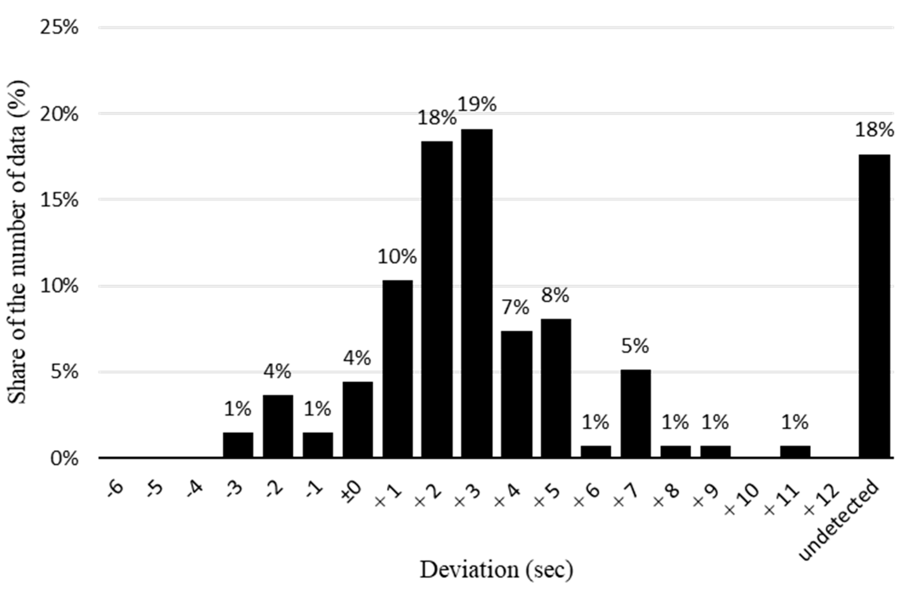
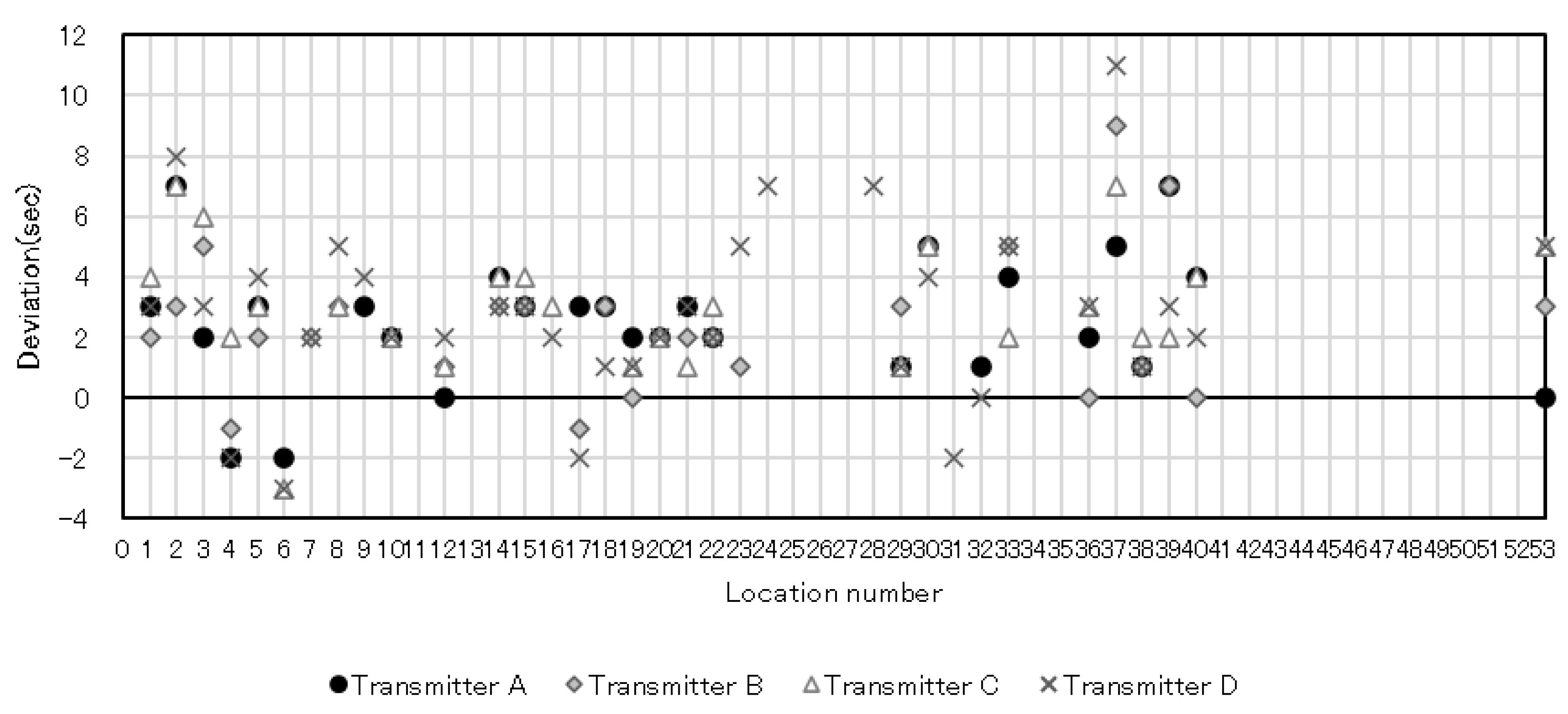
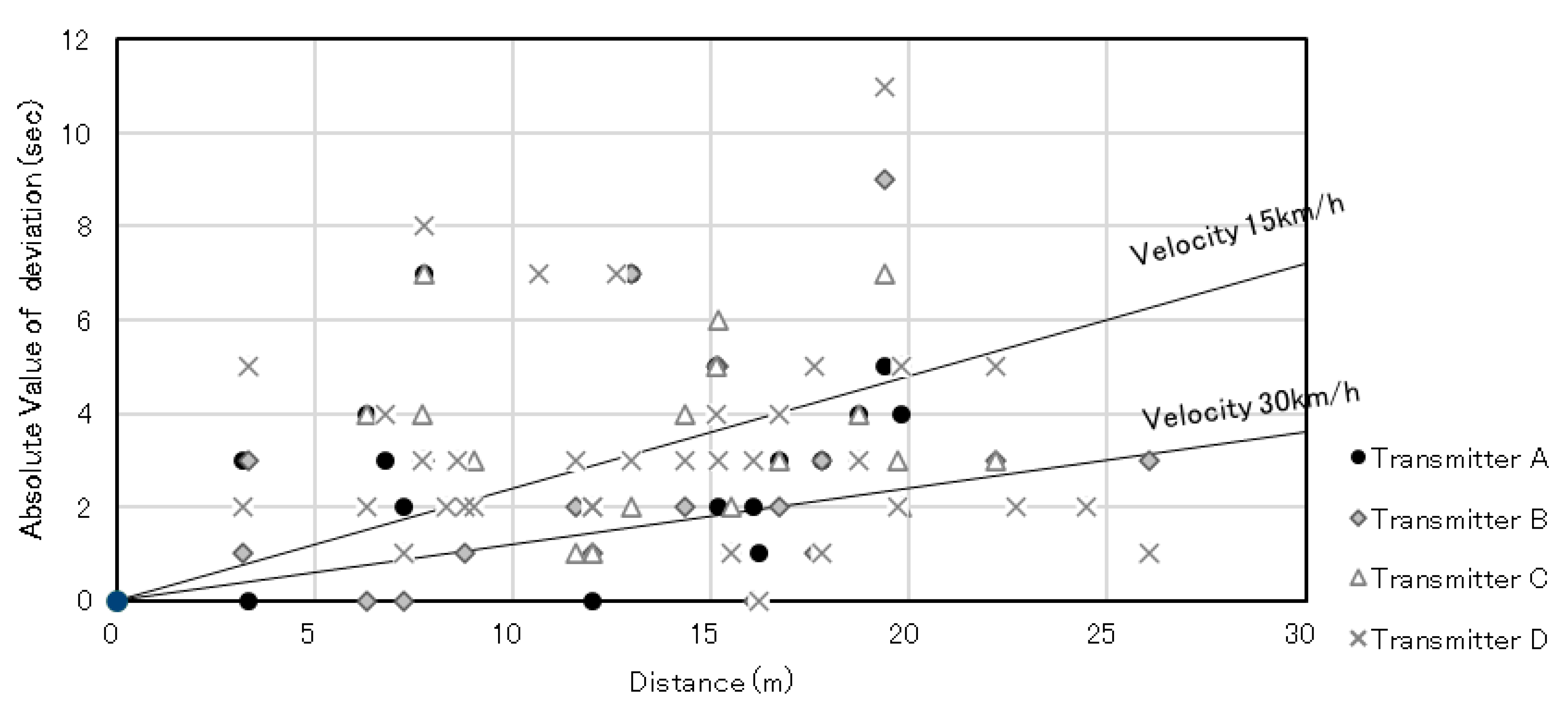
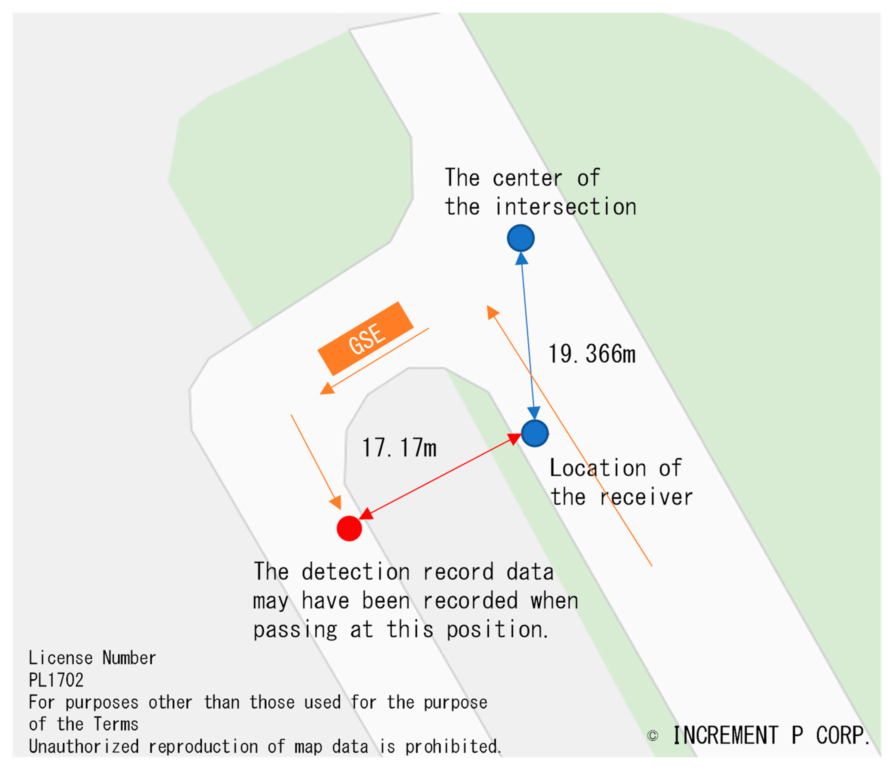
4.3. Discrepancy Between the Detection Time and Actual Passage Time of GSE
- The physical distance between the receiver’s location and the center of a nearby intersection.
- Individual differences and fluctuations in the BLE signal strength for each beacon.
- The BLE signals are detected at 2 s intervals; however, only detection data with the highest signal strength at 55 s intervals are actually recorded as the detection record data.
5. Discussion
6. Conclusions
Author Contributions
Funding
Data Availability Statement
Acknowledgments
Conflicts of Interest
Appendix A. Supplementary Data

| Vehicle Type Classification for Analysis | Number of Vehicles (Units) | Number of Detections (Cases) | Average Number of Detections (Cases/Unit) |
|---|---|---|---|
| Towing tractors | 455 | 694,205 | 1526 |
| Cargo vehicles | 354 | 555,813 | 1570 |
| Maintenance-related vehicles | 353 | 312,618 | 886 |
| Liaison vehicles | 295 | 495,383 | 1679 |
| Handling vehicles | 156 | 279,791 | 1794 |
| Refueling vehicles | 135 | 189,303 | 1402 |
| Catering vehicles | 116 | 79,318 | 684 |
| Aircraft towing vehicles | 105 | 165,902 | 1580 |
| Passenger transport buses | 71 | 105,903 | 1492 |
| Airport maintenance related vehicles | 62 | 46,258 | 746 |
| Passenger step vehicles | 53 | 26,995 | 509 |
| Non-handling freight transport vehicles | 40 | 2507 | 63 |
| Other vehicles | 39 | 57,715 | 1480 |
| Total of all vehicles | 2234 | 3,011,711 | 1348 |
References
- International Civil Aviation Organization (ICAO). Annual Report of the ICAO Council; International Civil Aviation Organization (ICAO): Montreal, QC, Canada, 2014. [Google Scholar]
- Air Transport Action Group (ATAG). Waypoint 2050, 2nd ed.; Air Transport Action Group (ATAG): Geneva, Switzerland, 2021. [Google Scholar]
- Eurocontrol. CODA Digest–Annual 2022. All-Causes Delays to Air Transport in Europe; Eurocontrol: Brussels, Belgium, 2022. [Google Scholar]
- Bureau of Transportation Statistics (BTS). Transportation Statistics Annual Report 2018; Bureau of Transportation Statistics (BTS): Washington, DC, USA, 2018. [Google Scholar]
- Bureau of Transportation Statistics (BTS). Transportation Statistics Annual Report 2020; Bureau of Transportation Statistics (BTS): Washington, DC, USA, 2020. [Google Scholar]
- Tabares, A.D. A Contribution to Automation of Airport Ground Operations. Ph.D. Thesis, Université Fédérale de Toulouse, Toulouse, France, 2018. (In French). [Google Scholar]
- Tabares, A.D.; Mora-Camino, F.; Drouin, A. A multi-time scale management structure for airport ground handling automation. J. Air Transp. Manag. 2021, 90, 101959. [Google Scholar] [CrossRef]
- Korkmaz, H.; Filazoglu, E.; Ates, S.S. Enhancing airport apron safety through intelligent transportation systems: Proposed FEDA model. Saf. Sci. 2023, 164, 106184. [Google Scholar] [CrossRef]
- Weiszer, M.; Chen, J.; Locatelli, G. An integrated optimisation approach to airport ground operations to foster sustainability in the aviation sector. Appl. Energy 2015, 157, 567–582. [Google Scholar] [CrossRef]
- Chikha, P.; Skorupski, J. The risk of an airport traffic accident in the context of the groundhandling personnel performance. J. Air Transp. Manag. 2022, 105, 102295. [Google Scholar] [CrossRef]
- Airport Research Center (ARC). Study on the Impact of Directive 96/67/EC on Ground Handling Services 1996–2007 Final Report; Airport Research Center: Aachen, Germany, 2009. [Google Scholar]
- Japan Civil Aviation Bureau (JCAB). Vision for Sustainable Development of Airport Operations Interim Summary. 2023. Available online: https://www.mlit.go.jp/koku/content/001614176.pdf (accessed on 20 September 2024). (In Japanese).
- Padrón, S.; Guimarans, D.; Ramos, J.J.; Fitouri-Trabelsi, S. A bi-objective approach for scheduling ground-handling vehicles in airports. Comput. Oper. Res. 2016, 71, 34–53. [Google Scholar] [CrossRef]
- Tabares, A.D.; Mora-Camino, F. Aircraft ground operations: Steps towards automation. CEAS Aeronaut. J. 2019, 10, 965–974. [Google Scholar] [CrossRef]
- Hájnik, A.; Harantová, V.; Kalašová, A. Use of electromobility and autonomous vehicles at airports in Europe and worldwide. Transp. Res. Procedia 2021, 55, 71–78. [Google Scholar] [CrossRef]
- Schiphol. Royal Schiphol Group Building a Road Map towards a Fully Autonomous Airside Operation in 2050. 2021. Available online: https://www.futuretravelexperience.com/2021/03/royal-schiphol-group-building-a-roadmap-towards-a-fully-autonomous-airside-operation-in-2050/ (accessed on 25 December 2023).
- Japan Civil Aviation Bureau (JCAB). The Promotion of Aviation Innovation. 2018. Available online: https://www.mlit.go.jp/koku/koku_tk19_000028.html (accessed on 25 December 2023). (In Japanese).
- Japan Civil Aviation Bureau (JCAB). 1st Meeting of the Field Operational Test Study Committee on Autonomous Driving in Restricted Areas of Airports. 2018. Available online: https://www.mlit.go.jp/koku/koku_tk9_000024.html (accessed on 25 December 2023). (In Japanese).
- Japan Civil Aviation Bureau (JCAB). 10th Meeting of the Study Committee for the Realization of Autonomous Driving in Restricted Areas of Airports. 2021. Available online: https://www.mlit.go.jp/koku/content/001445876.pdf (accessed on 20 September 2024). (In Japanese).
- Zhang, T.; Zhang, Z.; Zhu, X. Detection and control framework for unpiloted ground support equipment within the aircraft stand. Sensors 2024, 24, 205. [Google Scholar] [CrossRef]
- Yıldız, S.; Aydemir, O.; Memiş, A.; Varlı, S. A turnaround control system to automatically detect and monitor the time stamps of ground service actions in airports: A deep learning and computer vision-based approach. Eng. Appl. Artif. Intell. 2022, 114, 105032. [Google Scholar] [CrossRef]
- Thai, V.P.; Alam, S.; Lilith, N.; Tran, P.N.; Nguyen, B.T. Aircraft push-back prediction and turnaround monitoring by vision-based object detection and activity identification. In Proceedings of the 10th SESAR Innovation Days, Virtual, 7–10 December 2020. [Google Scholar]
- Lee, S.; Seo, S.W. Probabilistic context integration-based aircraft behaviour intention classification at airport ramps. IET Intell. Transp. Syst. 2022, 16, 725–738. [Google Scholar] [CrossRef]
- Thai, P.; Alam, S.; Lilith, N.; Nguyen, B.T. A computer vision framework using convolutional neural networks for airport-airside surveillance. Transp. Res. C 2022, 137, 103590. [Google Scholar] [CrossRef]
- Skorupski, J.; Grabarek, I.; Kwasiborska, A.; Czyżo, S. Assessing the suitability of airport ground handling agents. J. Air Transp. Manag. 2020, 83, 101763. [Google Scholar] [CrossRef]
- Liu, C.; Chen, Y.R.; Wang, H.; Zhang, Y.Y.; Dai, X.W.; Luo, Q.; Chen, L.Y. Airport flight ground service time prediction with missing data using graph convolutional neural network imputation and bidirectional sliding mechanism. Appl. Soft Comput. 2023, 133, 109941. [Google Scholar] [CrossRef]
- Evler, J.; Lindner, M.; Fricke, H.; Schultz, M. Integration of turnaround and aircraft recovery to mitigate delay propagation in airline networks. Comput. Oper. Res. 2022, 138, 105602. [Google Scholar] [CrossRef]
- Zhiwei, X.; Biao, L.; Hui, Z.; Qian, L. Research on flight ground service time prediction based on deep neural network. J. Syst. Simul. 2020, 32, 678. (In Chinese) [Google Scholar]
- Conte, C.; de Alteriis, G.; Schiano Lo Moriello, R.; Accardo, D.; Rufino, G. Drone trajectory segmentation for real-time and adaptive time-of-flight prediction. Drones 2021, 5, 62. [Google Scholar] [CrossRef]
- Eurocontrol. Airport CDM Implementation Manual. 2017. Available online: https://www.eurocontrol.int/publication/airport-collaborative-decision-making-cdm-implementation-manual (accessed on 25 December 2023).
- Akbar, M.C.; Pasa, I.T.; Permata, D.S.A. Use of CCTV to improve AMC unit supervision management ai Kualanamu international airport. J. Inf. Technol. Comput. Sci. Electr. Eng. 2024, 1, 35–37. [Google Scholar]
- Febiyanti, H.; Setiyo, S.; Kusdarwanto, H.; Azzahra, V.N. The impact of closed circuit television addition on apron movement control supervision in Apron C Juanda Airport. Proceeding Int. Conf. Adv. Transp. Eng. Appl. Soc. Sci. 2023, 2, 974–980. [Google Scholar] [CrossRef]
- Dewi, P.A.S.; Musadek, A.; Rinaldi, R. The analysis of personnel supervision functions apron movement control (AMC) efforts to reduce the rate of violation of ground support equipment (GSE) vehicle speed limits on the service road at Sam Ratulangi International Airport, Manado. Proceeding Int. Conf. Adv. Transp. Eng. Appl. Soc. Sci. 2023, 2, 798–805. [Google Scholar] [CrossRef]
- Castro, P. EU airport ground handling directive or when discretion interferes with public duty: A proposal on how to save Portugal’s transposition from discretion. Case Stu. Transp. Pol. 2022, 10, 1473–1482. [Google Scholar] [CrossRef]
- Patriarca, R.; Di Gravio, G.D.; Costantino, F. Assessing performance variability of ground handlers to comply with airport quality standards. J. Air Transp. Manag. 2016, 57, 1–6. [Google Scholar] [CrossRef]
- Japan Civil Aviation Bureau (JCAB). Airport Management Status Report. 2020. Available online: https://www.mlit.go.jp/koku/15_bf_000185.html (accessed on 25 December 2023). (In Japanese).
- Airports Council International (ACI). World Airport Traffic Dataset; Airports Council International (ACI): Montreal, QC, Canada, 2024. [Google Scholar]

| Location | Haneda Airport’s restricted area |
| Implementation period | 21–27 November 2019: 24 h × 7 d |
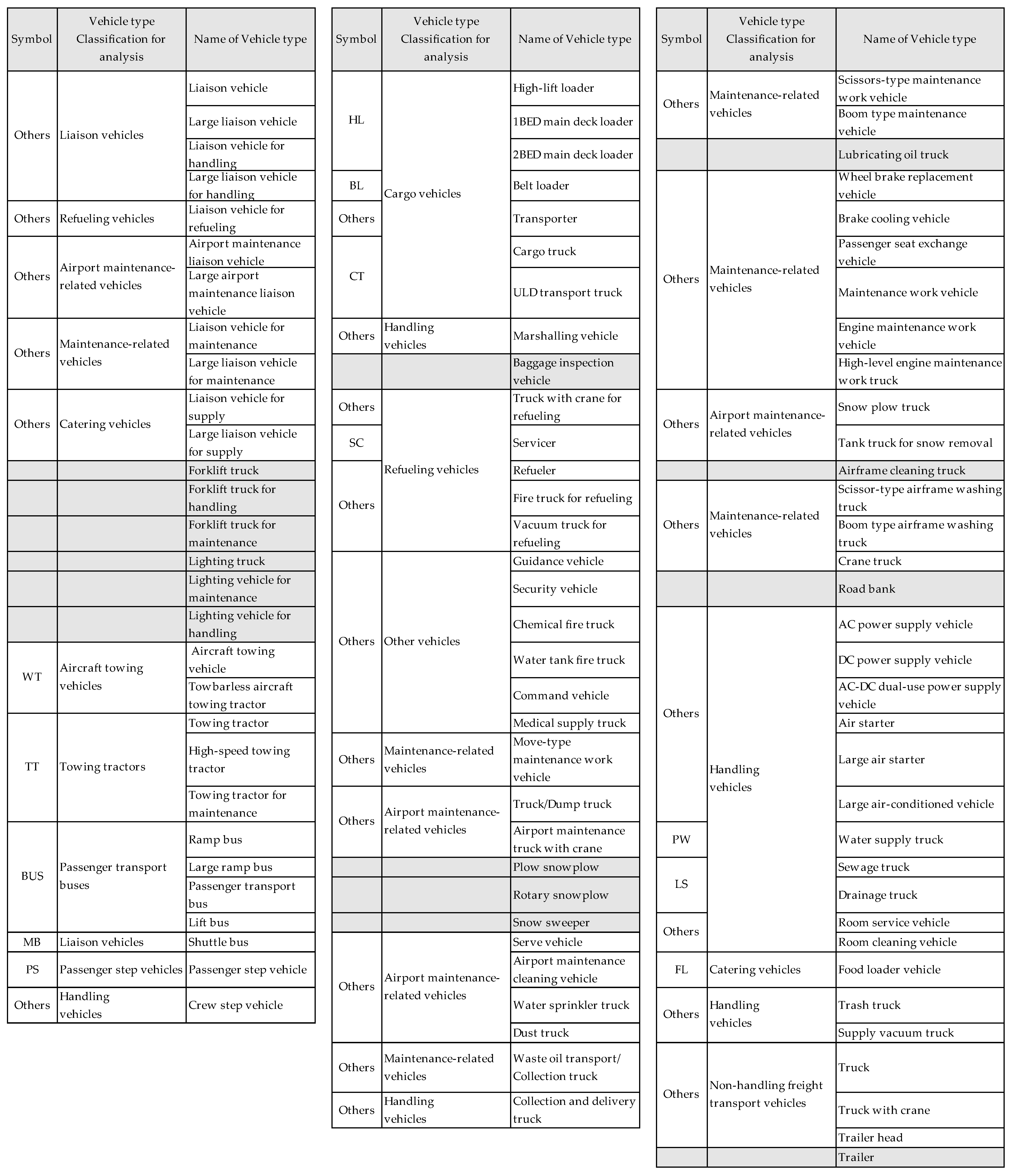
| Vehicles surveyed | All self-propelled GSE (except for some vehicle types such as forklifts and lighting vehicles), details are listed in Appendix A Figure A1 |
| Companies surveyed | 22 |
| Transmitters attached | 2234 vehicles (approximately 74% of the vehicles surveyed) |
| Receivers installed | 53 locations |
| Data obtained | Vehicle ID, passing position, and detection time data for GSE (hereinafter referred to as detection record data) |
| Classification of Vehicle Type | Number of GSE Vehicles Based on Detection Record Data (a) | Number of GSE Vehicles Recorded by Fixed-Point Camera (b) | (b)/(a) |
|---|---|---|---|
| Special heavy-duty vehicles | 7 | 15 | 2.14 |
| TT * | 559 | 837 | 1.50 |
| BUS/MB | 96 | 112 | 1.17 |
| Other vehicles | 348 | 147 | 0.42 |
| Total | 1010 | 1111 | 1.1 |
Disclaimer/Publisher’s Note: The statements, opinions and data contained in all publications are solely those of the individual author(s) and contributor(s) and not of MDPI and/or the editor(s). MDPI and/or the editor(s) disclaim responsibility for any injury to people or property resulting from any ideas, methods, instructions or products referred to in the content. |
© 2024 by the authors. Licensee MDPI, Basel, Switzerland. This article is an open access article distributed under the terms and conditions of the Creative Commons Attribution (CC BY) license (https://creativecommons.org/licenses/by/4.0/).
Share and Cite
Kuroda, Y.; Sato, S.; Hanaoka, S. Measurement of Driving Conditions of Aircraft Ground Support Equipment at Tokyo International Airport. Aerospace 2024, 11, 873. https://doi.org/10.3390/aerospace11110873
Kuroda Y, Sato S, Hanaoka S. Measurement of Driving Conditions of Aircraft Ground Support Equipment at Tokyo International Airport. Aerospace. 2024; 11(11):873. https://doi.org/10.3390/aerospace11110873
Chicago/Turabian StyleKuroda, Yuka, Satoshi Sato, and Shinya Hanaoka. 2024. "Measurement of Driving Conditions of Aircraft Ground Support Equipment at Tokyo International Airport" Aerospace 11, no. 11: 873. https://doi.org/10.3390/aerospace11110873
APA StyleKuroda, Y., Sato, S., & Hanaoka, S. (2024). Measurement of Driving Conditions of Aircraft Ground Support Equipment at Tokyo International Airport. Aerospace, 11(11), 873. https://doi.org/10.3390/aerospace11110873