Abstract
Advanced Aerial Mobility (AAM) platforms are poised to begin high-density operations in urban areas nationwide. This new category of aviation platforms spans a broad range of sizes, from small package delivery drones to passenger-carrying vehicles. Unlike traditional aircraft, AAM vehicles operate within the urban boundary layer, where large structures, such as buildings, interrupt the flow. This study examines the response of a package delivery drone, a general aviation aircraft, and a passenger-carrying urban air mobility aircraft through an urban wind field generated using Large Eddy Simulations (LES). Since it is burdensome to simulate flight dynamics in real-time using the full-order solution, reduced-order wind models are created. Comparing trajectories for each aircraft platform using full-order or reduced-order solutions reveals little difference; reduced-order wind representations appear sufficient to replicate trajectories as long as the spatiotemporal wind field is represented. However, examining control usage statistics and time histories creates a stark difference between the wind fields, especially for the lower wing-loading package delivery drone where control saturation was encountered. The control saturation occurrences were inconsistent across the full-order and reduced-order winds, advising caution when using reduced-order models for lightly wing-loaded aircraft. The results presented demonstrate the effectiveness of using a simulation environment to evaluate reduced-order models by directly comparing their trajectories and control activity metrics with the full-order model. This evaluation provides designers valuable insights for making informed decisions for disturbance rejection systems. Additionally, the results indicate that using Reynolds-averaged Navier–Stokes (RANS) solutions to represent urban wind fields is inappropriate. It was observed that the mean wind field trajectories fall outside the 95% confidence intervals, a finding consistent with the authors’ previous research.
1. Introduction
Technological challenges are a significant obstacle to the safe integration of future air vehicles categorized under Advanced Air Mobility (AAM), which are proposed to operate in high volumes in densely populated areas worldwide. The AAM revolution aims to introduce a broad spectrum of new vehicles, from package delivery drones to passenger-carrying aircraft that provide on-demand transportation [1,2,3,4]. Within the aeromechanics discipline, researchers are developing new tools and techniques to effectively simulate the complex interactions between the propulsive and aerodynamic elements of these vehicles, which operate in both vertical lift and wing-borne modes, as well as complex transition phases with high aerodynamic inflow angles [5]. Also vital is the representation of the relevant environments in which the air vehicle will operate to assess its safe operation accurately [6].
Simulating these conditions is critical for defining safe operational boundaries in AAM systems. However, there is a clear need to identify and test relevant urban wind environments and flight trajectories, as highlighted in Ref. [7]. Few studies have thoroughly investigated these interactions. For instance, Ref. [8] utilizes blade element momentum theory to simulate the aerodynamic performance of a quadcopter, but it does not explore the broader implications of urban turbulence on different vehicle types, such as fixed-wing configurations. Similarly, Ref. [9] focuses on aeroelastic considerations for a highly flexible fixed-wing aircraft yet omits urban-specific flight scenarios analysis. These limited studies underscore a significant gap in the literature, which our research aims to address by incorporating additional platforms and complex cityscape environments. The interaction between AAM systems and their operational environments is critical for certification, particularly in the absence of historical data [10].
Traditional turbulence models are not capable of representing the atmospheric dynamics in dense urban areas, especially phenomena due to interference effects from large obstructions like buildings or other artificial topographical features. Instead, well-known continuous and discrete gust models such as the von Karman and Dryden models aim to assess the vehicle in open-air flight [11]. Without readily available wind field models for urban environments, an alternative lies in using numerical simulations to capture wind fields around urban structures and the resulting interaction with an aircraft platform, especially within the atmospheric boundary layer. However, numerical simulations pose computational challenges associated with real-time predictions for operating AAM air vehicles. In contrast, reduced-order models (ROMs) or surrogate models are designed to approximate data from numerical simulations at reasonable accuracy [12,13]. These models and their extensions could enable both generating realistic wind data [14,15,16] for testing [17] and for predicting wind data using techniques like machine learning [18]. The Proper Orthogonal Decomposition (POD) method is widely used for extracting the richest modal information from a set of time-series data from experiments or simulations [19,20]. These modes can be used to obtain lower-dimensional dynamic models [21,22]; hence, this method was used to generate the reduced-order wind.
The primary contribution of this paper is to evaluate the suitability of using reduced-order urban wind models to analyze the flight performance of AAM vehicles across a spectrum of wing-loadings in close proximity to a large, isolated building. To this end, this paper expands the authors’ previous work [23] investigating the one-way coupled interactions between spatiotemporally varying wind fields and a flight dynamics model, which generates the resulting trajectories and controls usage time histories and metrics. The unsteady vortex lattice method (UVLM) [24,25] is employed to efficiently model three different fixed-wing platforms at various starting altitudes in the urban boundary layer as they traverse the computational domain while solving for overall forces and moments, including those due to unsteady wind fields. The turbulence due to the presence of buildings presents as a property of the operating environment, but aircraft response may vary greatly depending on vehicle size and wing-loading in particular [26,27]. Therefore, studying aircraft response across a range of wing-loadings can inform the capability of reduced-order wind models to replicate aircraft dynamics for simulation purposes.
2. Materials and Methods
2.1. Computational Fluid Dynamics Setup
Large Eddy Simulation (LES) was used to generate a realistic wind field using Open-source Field Operation and Manipulation (OpenFOAM) [28]. OpenFOAM is a numerical solver toolbox that can be used to perform CFD simulations for combustion, turbulence modeling, fluid flows, and other systems [29]. The Boussinesq-approximated incompressible Navier–Stokes equations are solved, and the LES closure model used is detailed in the sections below.
2.1.1. Governing Equations
The equations governing the flow of a viscous fluid with incompressibility assumption in a Cartesian coordinate system are the continuity and momentum equations. These are presented below as follows:
Filtering the above equations and after simplification, we obtain
However, it is impossible to determine the quantity , but the quantity is known. Substituting and using yields
where (with ) denotes the velocity components, and represents the sub-grid scale stress tensor.
Combined with the Boussinesq hypothesis, the sub-grid stress can be written as
where
, is the turbulent viscosity.
2.1.2. Turbulence Closure
The Wall-Adaptive Local Eddy-viscosity (WALE) model [30] is used for Sub Grid Scale (SGS) closure. The WALE model considers the effects of the turbulent wall surface and momentum transfer in contrast to the traditional Smogarinsky model. The expression for the turbulence viscosity is computed using
where is the filter scale determined by the lengths of the element in x, y, z directions, and is computed using
here,
2.1.3. Precursor Simulation Setup
A precursor Reynolds-averaged Navier–Stokes simulation (RANS) is set up based on the recommendations of Hargreaves et al. [31]. We adjust the domain of the precursor to match its outlet to the inlet face of the simulation while using the same grid spacing on the faces. A domain of length 5 km is chosen with an inlet wind profile specified using log-law with reference height () 50 m and 8 m/s wind speed at reference height. This follows the recommendations of Hargreaves et al. [31] to generate an atmospheric boundary layer. A roughness length () [32] is chosen for the ground plane. The inlet profile is set up using OpenFOAM’s atmBoundaryLayer boundary condition. atmNutkWallFunction wall function in OpenFOAM accounts for roughness in atmospheric boundary layer modeling.
2.1.4. Simulation Setup
The CFD domain size was chosen based on recommendations of Franke et al. [33]. The domain has a blockage ratio not exceeding 3%, 5H height above the building, 3H wide on sides of the building perpendicular to the flow direction, 5H length upstream, and 15H downstream where H m (the height of the building). Boone Pickens Stadium, positioned at 36°7′32.5″ N and a longitude of 97°4′1.7″ W, on the Oklahoma State University campus in Stillwater, Oklahoma, USA, was chosen as the building to be modeled in the CFD domain. Appropriate boundary conditions have been specified to the faces of the domain, and details about the domain mesh can be found in Table 1. For more details on the mesh generation, simulation, and validation of simulation, the interested reader is referred to Vuppala et al. [23].

Table 1.
Domain and mesh information of the simulation setup. For more details, see Vuppala et al. [23].
2.1.5. Flight Path Selection
The nominal flight path was chosen to be at the center of the domain flying upwind (UC), as shown in Figure 1 based on previous work [23]. To determine the heights at which the free stream atmospheric boundary layer airflow was influenced by the stadium, data were sampled along the height (lines) at different locations in the flow direction as depicted in Figure 2a. The half of the sum of variances of the fluctuating velocity components along these lines, averaged over time, is used as a measure to determine the flight levels. This measure is identical to averaged Turbulent Kinetic Energy (TKE) k computation when using Reynolds Decomposition and computed as shown in Equations (10)–(12). Based on the observations shown in Figure 2b, it could be inferred that the region influence seems to lie below 120 m, and hence, 45 m, 60 m, and 100 m heights were chosen for flight trajectory simulations.
where is the mean velocity vector,
where is the velocity vector with components
where k is the average turbulent kinetic energy.
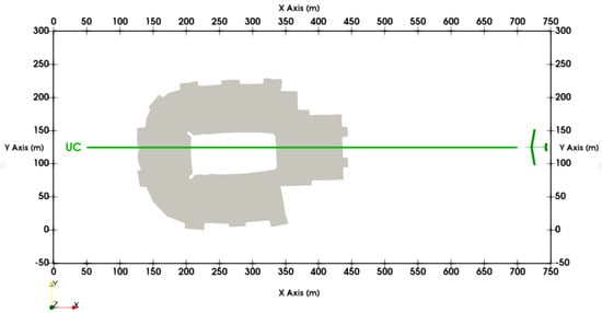
Figure 1.
Nominal path of the aircraft relative to the stadium (grey) for all altitudes.
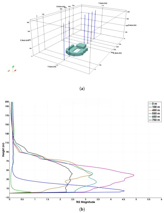
Figure 2.
Altitude determination using TKE metric. (a) A 3D view depicting the x-locations where line data was sampled relative to the building. (b) Average TKE along the height at various x-locations on the center of the domain (nominal flight path).
2.1.6. Reduced-Order Wind Generation
The Large Eddy Simulation data from the region of interest in the CFD domain as shown in Figure 2a are considered at one-second intervals for a total duration of 150 s. The interested reader is referred to our previous work, Vuppala et al. [23], but a brief overview is presented here. Using the Proper Orthogonal Decomposition [19,20] technique, the three-component velocity field from this region is used to obtain the orthogonal basis. The Relative Information Content (RIC) is computed as shown in Equation (13) and used as a criterion to decide the number of modes. Two values of RIC 50% and 80% were chosen, and the corresponding reduced-order wind was generated. The number of modes selected for each velocity component u, v, w is depicted in Figure 3. The overall schematic for reduced-order generation is depicted in Figure 4.
where is the relative information content for N modes, N is the cut-off number of modes determined by user-defined and represents the singular values.
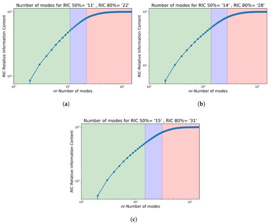
Figure 3.
Number of cut-off modes for RIC values 50% and 80%; Green—modes until 50%, Purple—modes from 50% to 80%, Red—neglected modes. Found for various velocity compenents: (a) u-velocity, (b) v-velocity, and (c) w-velocity.

Figure 4.
Schematic for reduced-order wind generation.
The amplitude versus frequency plots for three velocity components at an x-location of 550 m at an altitude of 60 m, corresponding to the full-order, 80%, and 50% RIC cases, are presented in Figure 5. The x-location is downstream of the building and lies on the nominal path shown in Figure 1. Fast Fourier Transform (FFT) was used to compute the amplitude and frequency of the velocity data at that location over the full time period of 150 s. Notably, reduced information content results in the loss of higher frequency information in the wind field.
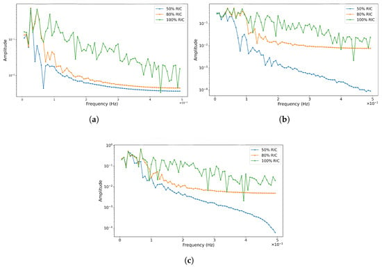
Figure 5.
Amplitude vs. Frequency at m, 60 m altitude on the nominal path. Amplitude vs. Frequency for (a) u-velocity components, (b) v-velocity components, and (c) w-velocity components.
2.2. Flight Dynamics
To simulate the aircraft’s response in 3D turbulent velocity fields, SHARPy [34] (Simulation of High-Aspect Ratio airplanes in Python) is employed. This code environment utilizes an unsteady vortex lattice method (UVLM) [35] to compute the distributed aerodynamic forces on the aircraft as it encounters the urban wind fields. The UVLM aerodynamic solver is derived from 3D potential flow theory, where the lifting surfaces are represented by distributed rectilinear vortex rings along the camber lines. The circulation strength around each vortex ring is found using Equation (14). A brief description of the UVLM used in SHARPy, and the implementation of the wind field within it will now be provided. A more detailed description is available in the authors’ previous work [23].
A non-penetrative boundary condition, Equations (14), is applied at each collocation point simultaneously to calculate the circulation strength vector (). This expression states that the normal velocity component to each collocation point must be zero, as air cannot penetrate a surface. The induced velocity contributions for both the bound and wake vortices are represented by aerodynamic influence coefficient (AIC) matrices ( and ), which are derived using the aircraft’s geometry and the Biot–Savart law. Normal velocities due to aircraft motion and turbulent gusts from the LES are incorporated using the term.
Within SHARPy, the unsteady formulation of the Kutta–Joukowski theorem [36] is used to find the aerodynamic forces. The steady and unsteady force contributions are represented by Equation (15) and (16) for a single vortex ring. All force components are then summed to find the total aerodynamic forces.
In accordance with the Kelvin condition, the trailing bound vortices of each aerodynamic surface transfer their vorticity to the wake panels. For this exercise, the convected-background-flow wake model is used as this model has been shown in previous studies that utilized SHARPy [37,38] to have equivalent rigid body trajectories when compared to the more computationally expensive full force-free wake model.
As in the previously published work, external wind fields are introduced to SHARPy using HDF5 [39] formatted files, which contain the time histories of the wind velocity magnitudes in the inertial frame and the corresponding spatial locations of the grid domain. The wind field is recorded at one-second intervals, and spatial and time interpolation is performed to define the disturbance gust magnitudes at each collocation point. The wind magnitudes are applied to the term in Equation (14), and the total aerodynamic forces and moments are found accordingly.
SHARPy incorporates an integration scheme to advance the models through wind fields, which has been used to generate the results presented here. A more detailed explanation of SHARPy’s application in propagating an aircraft through a Large Eddy Simulation (LES) field can be found in Ref. [9]. However, for the purposes of this paper, the structure is rigid, simplifying the notation. A summary of the simulation environment is shown below in Figure 6.

Figure 6.
Summary of SHARPy simulation environment.
2.3. Aircraft Models
Three platforms modeled in SHARPy represent configurations with high, medium, and low wing-loadings that span the extent of vehicles that fall under the AAM spectrum. Each configuration features uniform mass distributions across all components, arranged to achieve a static margin of to ensure dynamic stability. The mass moments of inertia are calculated based on these assumed mass distributions. Capturing every complex detail of the referenced platforms is beyond the scope of this exercise. Instead, simplifications have been made where appropriate, resulting in models whose inertial properties differ by at least one order of magnitude. Additionally, all control surfaces for each configuration have saturation limits of for simplicity. Although saturation limits are typically specific to each configuration, using the same values for each model will not significantly affect the results.
2.3.1. NASA AAM Concept
An Advanced Air Mobility (AAM) platform, initially described by NASA [2,40], is adopted as the high wing-loaded configuration for this exercise. This platform was represented in SHARPy in the previous efforts by the authors, [23], the findings that motivate this study. Results for the NASA AAM concept are presented at 45 m and 100 m altitudes. The previous results were only obtained at 60 m. In the current study, the initial condition at 60 m altitude was re-evaluated under comparable wind conditions, yielding similar overall trajectory response characteristics as reported earlier. The locations of lumped mass representations of the propulsion system are incorporated into the model and are shown in Figure 7. Table 2 summarizes the mass properties, assumed initial airspeed, and the airfoils for each aerodynamic surface.
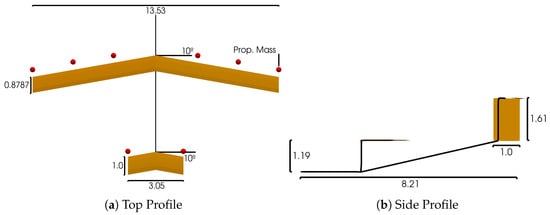
Figure 7.
Passenger-carrying AAM vehicle planform, shown in orange. All dimensions in m. Propulsion mass elements represented by red points.

Table 2.
Properties of the AAM vehicle.
2.3.2. Cessna 152
For the medium wing-loaded configuration, a simplified representation of a Cessna 152 was created in the SHARPY framework, as shown in Figure 8. Previous authors have used the aircraft for flight dynamics analysis cases [41]. For simplicity in the current implementation, taper and sweep are ignored on all lifting surfaces, but the relative sizing and longitudinal locations of wings are maintained. Airfoil profiles, target trim airspeed, and mass distribution properties are specified in Table 3.
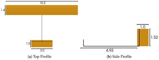
Figure 8.
Simplified Cessna 152 platform, shown in orange. All dimensions in m.

Table 3.
Properties of simplified Cessna 152 model.
2.3.3. Fixed-Wing Delivery Drone
The smallest configuration analyzed is the Zipline delivery drone, which has been utilized for delivering medical supplies in regions of Africa with limited transit infrastructure [42]. Due to the scarcity of detailed design parameters for the Zipline, the planform was reconstructed based on photographs and publicly available information, including estimates of airspeed and total mass. This delivery drone features a v-tail ruddervator, adapted as depicted in Figure 9. The v-tail has been projected onto the appropriate planes to create a conventional control surface layout. Table 4 summarizes all additional assumptions in creating the SHARPy model.

Figure 9.
Representative fixed-wing delivery drone planform, shown in orange. All dimensions in m.

Table 4.
Properties of the delivery drone vehicle.
3. Results
The nominal path of each aircraft through every wind field (Full-Order Model (FOM), 80%, 50%, and mean) resembles Figure 1 for all initial altitudes ranging from 45 m to 100 m. The mean wind field is the temporal average at each location in the FOM wind field, Equation (11). Spatial variation still exists for the mean wind field, and this case represents a Reynolds-averaged Navier–Stokes (RANS) representation. This case was included to further support the conclusions from the author’s previous effort [23]. It should be noted that the upper extent of the stadium is 40 m. This flight path is designated as UC (Upstream, Center) because the aircraft navigates upstream relative to the direction of the bulk flow. The starting location was chosen as it proved to be the most active and impactful of the locations studied in the previous efforts of the authors [23].
To identify statistical disparities between the responses of each configuration, 95% confidence intervals on the trajectory datasets are used. The 95% confidence intervals are determined using Student’s T-statistic (t), the sample size (n), and the standard deviation () of the dataset to evaluate Equation (17) [43].
To reduce variations in altitude and roll attitude, proportional gain controllers are implemented across all configurations, as detailed in Table 5. For simplicity, actuator dynamics, such as the inclusion of rate limiters, were ignored as this capability was not natively supported in the SHARPy environment. Each control surface is subject to a saturation limit of for every configuration. However, the control effectiveness varies among platforms due to differences in the size and placement of control surfaces relative to the center of gravity. These variations make it challenging to directly compare the performance of the control systems. Addressing this issue could involve more advanced control law design techniques; however, this approach falls outside the scope of this paper, which primarily aims to assess the impact of the different wind field models.

Table 5.
Feedback control gains.
The wind field data were captured at one-second intervals for 150 s. Each simulation is initiated at a start time of zero seconds, with subsequent simulations beginning at increments of 10 s. Due to variations in the speeds of the different configurations, the total number of recorded cases varies: 15 sets for the AAM with a flight duration of approximately 9 s, 14 sets for the Cessna with a duration of around 11 s per flight, and 13 sets for the delivery drone platform, with each flight taking about 22 s.
The most significant differences in longitudinal trajectories among the configurations were observed at an altitude of 60 m. Confidence intervals for these trajectories through the FOM wind field are illustrated in Figure 10. The responses of each configuration to the various wind fields (FOM, 80%, and 60%) at altitudes of 45 m, 60 m, and 100 m are shown in the following sections.

Figure 10.
All configurations confidence interval trajectories at 60 m through the FOM wind field.
3.1. High Average TKE: 45 m Altitude Trajectories
The 95% confidence interval trajectories at 45 m altitude are shown below in Figure 11, Figure 12 and Figure 13, illustrating the influence of the FOM, 80%, and 60% wind fields on both longitudinal and lateral responses. This altitude is the closest to the stadium, yet the trajectories are not as varied as the trajectories shown in the 60 m Altitude Trajectories section. The control activity at this altitude, though, as illustrated by the Lateral Response of the configurations, was the most active. This is particularly true for the delivery drone configuration, which featured several instances of control saturation. Control activity for the delivery drone is further discussed in the Control Surface Activity section.
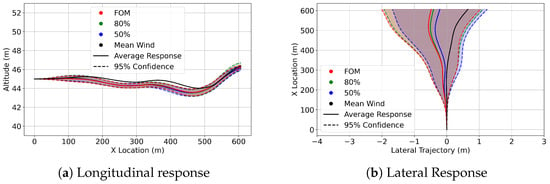
Figure 11.
AAM confidence interval trajectories at 45m in FOM wind (red), 80% ROM wind (green), 50% ROM wind (blue), and trajectory in the mean wind (black).
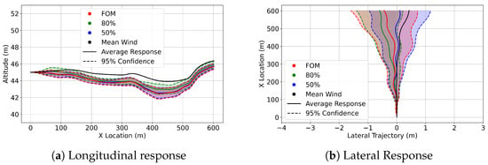
Figure 12.
Cessna 152 confidence interval trajectories at 45m in FOM wind (red), 80% ROM wind (green), 50% ROM wind (blue), and trajectory in the mean wind (black).
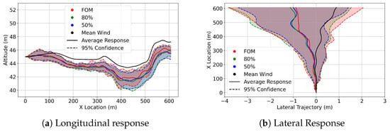
Figure 13.
Delivery drone confidence interval trajectories at 45m in FOM wind (red), 80% ROM wind (green), 50% ROM wind (blue), and trajectory in the mean wind (black).
3.2. Moderate Average TKE: 60 m Altitude Trajectories
The most significant altitude variations encountered amongst all datasets were observed at 60 m. This is supported by the 95% confidence interval trajectories shown in Figure 14, Figure 15 and Figure 16.
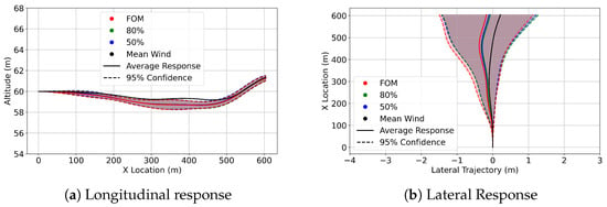
Figure 14.
AAM confidence interval trajectories at 60m in FOM wind (red), 80% ROM wind (green), 50% ROM wind (blue), and trajectory in the mean wind (black).
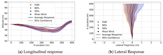
Figure 15.
Cessna 152 confidence interval trajectories at 60m in FOM wind (red), 80% ROM wind (green), 50% ROM wind (blue), and trajectory in the mean wind (black).
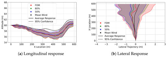
Figure 16.
Delivery drone confidence interval trajectories at 60m in FOM wind (red), 80% ROM wind (green), 50% ROM wind (blue), and trajectory in the mean wind (black).
3.3. Low Average TKE: 100 m Altitude Trajectories
At 100 m, the highest altitude in this study, it is observed from Figure 17, Figure 18 and Figure 19 that the influence of the wind fields has greatly diminished. This is shown in the longitudinal and Lateral Responses, which feature more narrow and concentrated flight paths.
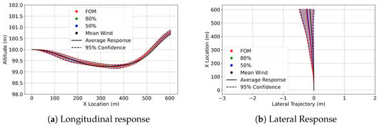
Figure 17.
AAM confidence interval trajectories at 100 m in FOM wind (red), 80% ROM wind (green), 50% ROM wind (blue), and trajectory in the mean wind (black).
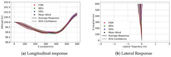
Figure 18.
Cessna confidence interval trajectories at 100m in FOM wind (red), 80% ROM wind (green), 50% ROM wind (blue), and trajectory in the mean wind (black).
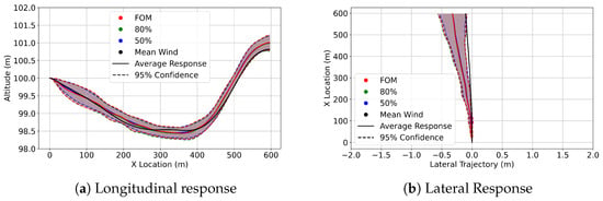
Figure 19.
Delivery drone confidence interval trajectories at 100m in FOM wind (red), 80% ROM wind (green), 50% ROM wind (blue), and trajectory in the mean wind (black).
3.4. Control Surface Activity
Table 6 and Table 7 present the standard deviations of the control surface activity for elevators and ailerons for every altitude, configuration, and wind field. The standard deviation of control deflections throughout a maneuver’s time history serves as a measure of control activity [44] and is an additional way to compare the responses of the configurations across the FOM and ROM wind fields. For the three aircraft models, control saturation for the elevator and aileron is taken as a deflection off of the neutral condition. In the simple feedback models utilized, no deflection is applied beyond this threshold.

Table 6.
Aileron standard deviations.

Table 7.
Elevator standard deviations.
The control usage time history for the delivery drone vehicle at 45 m across the FOM, 80%, and 50% wind fields is shown below in Figure 20. In this figure, the control surface deflections of each dataset are appended to each other; thus, the x-axis is left unlabeled for simplicity. Due to the delivery drone having the smallest inertial properties and lightest wing-loading, the control deflection featured the highest magnitudes across all configurations to maintain a controlled trajectory through the wind fields. Additionally, we see several instances of control saturation, noted to be an indicator of loss of control [45], in the FOM and 80% winds, yet none in the 50% and the mean cases as shown in Table 8.
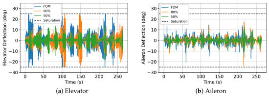
Figure 20.
Delivery drone control surface deflection history for every run case at 45 m.

Table 8.
Package delivery drone elevator control saturation encounters at each altitude.
4. Discussion
As observed in the previous work of the authors [23], the control activity for all mean wind cases is lower compared to the FOM and ROM cases as shown in Table 6 and Table 7. The results again suggest that a wind field that varies in time and space is essential for accurately capturing flight dynamics and control usage instead of employing a mean wind or wind field generated by a Reynolds-averaged Navier–Stokes (RANS) simulation.
The results show that the different wing-loadings and inertial properties of the configurations impacted the influence of the FOM and ROM wind fields on the trajectories. Specifically, when analyzing all configurations under the FOM wind field at 60 m, as shown in Figure 10, it is evident that platforms with lower inertial properties underwent more significant perturbations. Notably, the delivery drone was most affected, displaying the largest confidence intervals and the greatest deviation from initial conditions. This indicates that enhancing the design of disturbance rejection controllers is crucial, particularly for small delivery drones operating in urban settings. In contrast, larger passenger-carrying designs appear less affected by such disturbances.
The effects of the ROM wind fields, in comparison to the FOM, are depicted across the various altitudes and configurations as shown in Figure 11, Figure 12, Figure 13, Figure 14, Figure 15, Figure 16, Figure 17, Figure 18 and Figure 19. The differences seen on the trajectories are minor for all configurations, with 80% and 50% overall representative of the FOM response, with the most noticeable differences seen in the lateral responses. Although significant discrepancies in trajectories are not observed, there are notable variations in control activity across different configurations. The standard deviations in control deflections, which indicate variability in control activity, are the largest magnitudes at 45 m altitude, as illustrated in Table 6 and Table 7. This suggests heightened control efforts at this altitude to maintain a controlled flight path. Additionally, the differences between the standard deviations of the FOM and ROM responses increase as the wing-loading of the aircraft decreases, indicating differences in the control activity when comparing the FOM and ROM winds. This is reinforced by Figure 20, which shows apparent differences in the elevator deflection time histories of the delivery drone amongst the FOM, 80%, and 50% cases.
The data in Table 8 reveal inconsistent occurrences of control saturation across various fidelity wind fields, which is concerning due to the previously noted implication whereby control saturation implies a loss of control. For instance, at an altitude of 45 m, the delivery drone experiences control saturation six times in the FOM and five times in the 80% wind field but not at all in the 50% and mean wind fields. This inconsistency increases at 60 m, where the drone encounters control saturation 14 times in the FOM but only twice in the 80% field and never in the others. These results suggest that the ROMs lack the capability to accurately replicate the control activity observed in the FOM when the aircraft is highly perturbed, as in the case of the lightest wing-loading considered.
5. Future Research Directions
Based on the findings from this paper, future work will consist of taking the delivery drone platform and applying a more robust control architecture in an attempt to more effectively navigate the urban wind fields from a representative cityscape. Additionally, actuator dynamics will be considered to more accurately capture the practical challenges of controller implementation. The control architecture in use will be from the Ardupilot [46] library, which is a common autopilot software suite in the unmanned vehicle community. Ardupilot will be used to navigate the platform around the cityscape at different locations, azimuths, and altitudes and troubling locations in the wind field will be identified based on the response of the aircraft. Differences between the aircraft response in the FOM and ROMs will also be evaluated. This exercise will further highlight implementation issues that can be expected when deploying disturbance rejection systems on AAM platforms and the modeling considerations required to effectively and efficiently simulate the effects of urban wind fields.
The simulation framework developed in this work provides a strong foundation for exploring key topics such as gust rejection, obstacle avoidance, and wake interactions between aircraft in close proximity [47]. Future work can expand on this by implementing custom control architectures tailored to specific mission objectives [48]. Additionally, integrating aerodynamic models will enable the simulation of rotorcraft platforms, such as quadcopters.
6. Conclusions
The results indicate that careful consideration must be given to the use of ROM wind models to represent complex urban wind fields before they can be implemented in a manner that generates valid results. Validation cases using the FOM wind fields are highly recommended. This is particularly crucial for disturbance characterization in aircraft with low wing-loading. Although ROM wind fields offer significant advantages in terms of computational efficiency and data size, analysts must consider the appropriateness of the reduced-order wind models, especially if they are being used to identify the safe operating envelope for the vehicle in the proximity of large structures that greatly disturb the flow. The findings suggest that lightweight delivery drones either require more effective disturbance rejection control to navigate urban wind fields without frequently utilizing all available control power or need their operational envelope restricted to avoid flights near urban structures when the mean wind exceeds 8 m/s. If only the ROM wind fields were considered, the safe vehicle operating envelope for the delivery drone, when operating very close to the structure, would potentially include conditions known to lead to loss of control. The larger, more highly wing-loaded platforms perform nearly equivalently in the FOM and ROM wind fields, even when very close to the structure, suggesting that safe operating envelopes for the larger platforms could be evaluated using the ROM disturbance representations in the conditions modeled in this work.
Author Contributions
R.P. and K.K. conceived the experiment, Z.K. and R.K.S.S.V. conducted the numerical study. All authors have read and agreed to the published version of the manuscript.
Funding
Partial funding for this study was provided by National Science Foundation (NSF) Grant No. 1925147.
Data Availability Statement
The data supporting this study’s findings and additional details to replicate are available upon request to the corresponding author.
Acknowledgments
R.K.S.S.V. and K.K. acknowledge support from the National Science Foundation (NSF) under Grant No. 1925147. Any opinions, findings, and conclusions, or recommendations expressed in this material are those of the author(s) and do not necessarily reflect the views of the National Science Foundation. Some of the computing for this project was performed at the High-Performance Computing Center (HPCC) at Oklahoma State University, supported, in part, through the National Science Foundation (Grant No. OAC-1531128). Z.K. acknowledges support from the Department of Defense (DoD) SMART (Science, Mathematics, and Research for Transformation) scholarship program. The SMART scholarship is funded by: OUSD/R&E (The Under Secretary of Defense-Research and Engineering), National Defense Education Program (NDEP)/BA-1, Basic Research.
Conflicts of Interest
The authors declare no conflicts of interest.
References
- Frachtenberg, E. Practical drone delivery. Computer 2019, 52, 53–57. [Google Scholar] [CrossRef]
- Johnson, W.; Silva, C. NASA concept vehicles and the engineering of advanced air mobility aircraft. Aeronaut. J. 2022, 126, 59–91. [Google Scholar] [CrossRef]
- Goyal, R.; Reiche, C.; Fernando, C.; Cohen, A. Advanced air mobility: Demand analysis and market potential of the airport shuttle and air taxi markets. Sustainability 2021, 13, 7421. [Google Scholar] [CrossRef]
- Goyal, R.; Cohen, A. Advanced air mobility: Opportunities and challenges deploying eVTOLs for air ambulance service. Appl. Sci. 2022, 12, 1183. [Google Scholar] [CrossRef]
- Simmons, B.M.; Murphy, P.C. Aero-propulsive modeling for tilt-wing, distributed propulsion aircraft using wind tunnel data. J. Aircr. 2022, 59, 1162–1178. [Google Scholar] [CrossRef]
- Kopasakis, G. Atmospheric Turbulence Modeling for Aero Vehicles: Fractional Order Fits; Technical report; NASA: Washington, DC, USA, 2015. [Google Scholar]
- Connors, M.M. Understanding Risk in Urban Air Mobility: Moving towards Safe Operating Standards; NASA: Washington, DC, USA, 2020. [Google Scholar]
- Kakavitsas, N.; Willis, A.; Jacobik, R.; Uddin, M.; Wolek, A. Quadrotor Flight Simulation in a CFD-generated Urban Wind Field. In Proceedings of the 2024 IEEE Aerospace Conference, Big Sky, MT, USA, 2–9 March 2024; IEEE: Piscataway, NJ, USA, 2024; pp. 1–8. [Google Scholar]
- Del Carre, A.; Deskos, G.; Palacios, R. Realistic turbulence effects in low altitude dynamics of very flexible aircraft. In Proceedings of the AIAA Scitech 2020 Forum, Orlando, FL, USA, 6–10 January 2020; p. 1187. [Google Scholar]
- Patterson, M.D.; Isaacson, D.R.; Mendonca, N.L.; Neogi, N.A.; Goodrich, K.H.; Metcalfe, M.; Bastedo, B.; Metts, C.; Hill, B.P.; DeCarme, D.; et al. An initial concept for intermediate-state, passenger-carrying urban air mobility operations. In Proceedings of the AIAA Scitech 2021 Forum, Online, 11–15, 19–21 January 2021; p. 1626. [Google Scholar]
- Wu, Z.; Cao, Y.; Ismail, M. Gust loads on aircraft. Aeronaut. J. 2019, 123, 1216–1274. [Google Scholar] [CrossRef]
- Qian, Z.; Seepersad, C.C.; Joseph, V.R.; Allen, J.K.; Jeff Wu, C. Building surrogate models based on detailed and approximate simulations. J. Mech. Des. 2006. [Google Scholar] [CrossRef]
- Alizadeh, R.; Allen, J.K.; Mistree, F. Managing computational complexity using surrogate models: A critical review. Res. Eng. Des. 2020, 31, 275–298. [Google Scholar] [CrossRef]
- Vuppala, R.K.; Kara, K. A non-intrusive reduced order model using deep learning for realistic wind data generation for small unmanned aerial systems in urban spaces. AIP Adv. 2022, 12, 085020. [Google Scholar] [CrossRef]
- Vuppala, R.K.; Kara, K. Wind Field Prediction in Urban Spaces for small Unmanned Aerial Systems using Convolutional Autoencoders. In Proceedings of the AIAA AVIATION 2022 Forum, Chicago, IL, USA, 27 June–1 July 2022; p. 3605. [Google Scholar]
- Vuppala, R.K.; Kara, K. A Novel Approach in Realistic Wind Data Generation for The Safe Operation of Small Unmanned Aerial Systems in Urban Environment. In Proceedings of the AIAA AVIATION 2021 Forum, Online, 2–6 August 2021; p. 2505. [Google Scholar]
- Tabassum, A.; Vuppala, R.K.; Bai, H.; Kara, K. Variance reduction of quadcopter trajectory tracking in turbulent wind. IFAC-PapersOnLine 2021, 54, 102–107. [Google Scholar] [CrossRef]
- Vuppala, R.K.; Kara, K. Deep Learning for Realistic Wind Field Prediction in a typical Urban Morphology for Application to Small Unmanned Aerial Systems. In Proceedings of the AIAA SCITECH 2023 Forum, National Harbor, MD, USA, 23–27 January 2023; p. 1757. [Google Scholar]
- Berkooz, G.; Holmes, P.; Lumley, J.L. The proper orthogonal decomposition in the analysis of turbulent flows. Annu. Rev. Fluid Mech. 1993, 25, 539–575. [Google Scholar] [CrossRef]
- Chatterjee, A. An introduction to the proper orthogonal decomposition. Curr. Sci. 2000, 78, 808–817. [Google Scholar]
- Liang, Y.; Lee, H.; Lim, S.; Lin, W.; Lee, K.; Wu, C. Proper orthogonal decomposition and its applications—Part I: Theory. J. Sound Vib. 2002, 252, 527–544. [Google Scholar] [CrossRef]
- Volkwein, S. Proper Orthogonal Decomposition: Theory and Reduced-Order Modelling; Lecture Notes; University of Konstanz: Konstanz, Germany, 2013; Volume 4, pp. 1–29. [Google Scholar]
- Vuppala, R.K.; Krawczyk, Z.; Paul, R.; Kara, K. Modeling advanced air mobility aircraft in data-driven reduced order realistic urban winds. Sci. Rep. 2024, 14, 383. [Google Scholar] [CrossRef] [PubMed]
- Paul, R.C.; Murua, J.; Gopalarathnam, A. Unsteady and post-stall aerodynamic modeling for flight dynamics simulation. In Proceedings of the AIAA Atmospheric Flight Mechanics Conference, National Harbor, MD, USA 13–17 January 2014; p. 0729. [Google Scholar]
- Murua, J.; Palacios, R.; Graham, J.M.R. Applications of the unsteady vortex-lattice method in aircraft aeroelasticity and flight dynamics. Prog. Aerosp. Sci. 2012, 55, 46–72. [Google Scholar] [CrossRef]
- Nelson, R.C. Flight Stability and Automatic Control; WCB/McGraw Hill: New York, NY, USA, 1998; Volume 2. [Google Scholar]
- Cornman, L.B.; Morse, C.S.; Cunning, G. Real-time estimation of atmospheric turbulence severity from in-situ aircraft measurements. J. Aircr. 1995, 32, 171–177. [Google Scholar] [CrossRef]
- Jasak, H.; Jemcov, A.; Tukovic, Z. OpenFOAM: A C++ library for complex physics simulations. In Proceedings of the International Workshop on Coupled Methods in Numerical Dynamics, Dubrovnik, Croatia, 19–21 September 2007; Volume 1000, pp. 1–20. [Google Scholar]
- Chen, G.; Xiong, Q.; Morris, P.J.; Paterson, E.G.; Sergeev, A.; Wang, Y. OpenFOAM for computational fluid dynamics. Not. Ams 2014, 61, 354–363. [Google Scholar] [CrossRef]
- Nicoud, F.; Ducros, F. Subgrid-scale stress modelling based on the square of the velocity gradient tensor. Flow Turbul. Combust. 1999, 62, 183–200. [Google Scholar] [CrossRef]
- Hargreaves, D.; Wright, N.G. On the use of the k–ε model in commercial CFD software to model the neutral atmospheric boundary layer. J. Wind. Eng. Ind. Aerodyn. 2007, 95, 355–369. [Google Scholar] [CrossRef]
- Cindori, M.; Juretić, F.; Kozmar, H.; Džijan, I. Steady RANS model of the homogeneous atmospheric boundary layer. J. Wind. Eng. Ind. Aerodyn. 2018, 173, 289–301. [Google Scholar] [CrossRef]
- Franke, J.; Hellsten, A.; Schlünzen, H.; Carissimo, B. Best Practice Guideline for the CFD Simulation of Flows in the Urban Environment. Ph.D. Thesis, COST European Cooperation in Science and Technology, Brussels, Belgium, 2007. [Google Scholar]
- del Carre, A.; Muñoz-Simón, A.; Goizueta, N.; Palacios, R. SHARPy: A dynamic aeroelastic simulation toolbox for very flexible aircraft and wind turbines. J. Open Source Softw. 2019, 4, 1885. [Google Scholar] [CrossRef]
- Katz, J.; Plotkin, A. Low-Speed Aerodynamics; Cambridge University Press: Cambridge, UK, 2001; Volume 13. [Google Scholar]
- Simpson, R.J.; Palacios, R.; Murua, J. Induced-drag calculations in the unsteady vortex lattice method. AIAA J. 2013, 51, 1775–1779. [Google Scholar] [CrossRef]
- Deskos, G.; del Carre, A.; Palacios, R. Assessment of low-altitude atmospheric turbulence models for aircraft aeroelasticity. J. Fluids Struct. 2020, 95, 102981. [Google Scholar] [CrossRef]
- Del Carre, A.; Palacios, R. Efficient Time-Domain Simulations in Nonlinear Aeroelasticity. In Proceedings of the 2019 AIAA SciTech Forum, San Diego, CA, USA, 7–11 January 2019. [Google Scholar]
- Koranne, S.; Koranne, S. Hierarchical data format 5: HDF5. In Handbook of Open Source Tools; Springer: Berlin/Heidelberg, Germany, 2011; pp. 191–200. [Google Scholar]
- Whiteside, S.; Pollard, B. Conceptual Design of a Tiltduct Reference Vehicle for Urban Air Mobility. In Proceedings of the Aeromechanics for Advanced Vertical Flight Technical Meeting, San Jose, CA, USA, 25–27 January 2022. [Google Scholar]
- Bunge, R.; Kroo, I. Compact formulation of nonlinear inviscid aerodynamics for fixed-wing aircraft. In Proceedings of the 30th AIAA Applied Aerodynamics Conference, New Orleans, LA, USA, 25–28 June 2012; p. 2771. [Google Scholar]
- Ackerman, E.; Koziol, M. The blood is here: Zipline’s medical delivery drones are changing the game in Rwanda. IEEE Spectr. 2019, 56, 24–31. [Google Scholar] [CrossRef]
- Navidi, W.C. Statistics for Engineers and Scientists; McGraw-Hill: New York, NY, USA, 2006; Volume 2. [Google Scholar]
- Paul, R.; Rhinehart, M. Exploring pilot workload using inceptor time histories. In Proceedings of the Vertical Flight Society’s 76th Annual Forum and Technology Display, Online, 5–8 October 2020. [Google Scholar]
- Wilborn, J.; Foster, J. Defining commercial transport loss-of-control: A quantitative approach. In Proceedings of the AIAA Atmospheric Flight Mechanics Conference and Exhibit, Providence, RI, USA, 16–19 August 2004; p. 4811. [Google Scholar]
- ArduPilot. 2024. Available online: https://ardupilot.org/ (accessed on 1 January 2024).
- Phadke, A.; Medrano, F.A.; Chu, T.; Sekharan, C.N.; Starek, M.J. Modeling Wind and Obstacle Disturbances for Effective Performance Observations and Analysis of Resilience in UAV Swarms. Aerospace 2024, 11, 237. [Google Scholar] [CrossRef]
- Chodnicki, M.; Siemiatkowska, B.; Stecz, W.; Stępień, S. Energy efficient UAV flight control method in an environment with obstacles and gusts of wind. Energies 2022, 15, 3730. [Google Scholar] [CrossRef]
Disclaimer/Publisher’s Note: The statements, opinions and data contained in all publications are solely those of the individual author(s) and contributor(s) and not of MDPI and/or the editor(s). MDPI and/or the editor(s) disclaim responsibility for any injury to people or property resulting from any ideas, methods, instructions or products referred to in the content. |
© 2024 by the authors. Licensee MDPI, Basel, Switzerland. This article is an open access article distributed under the terms and conditions of the Creative Commons Attribution (CC BY) license (https://creativecommons.org/licenses/by/4.0/).