Development of Aerodynamic and Propulsion Models Using the Iterative Equation Error Method

Abstract

For developing high-fidelity flight simulations, an accurate and complete representation of the aerodynamic characteristics of the aircraft is necessary. To obtain a realistic aerodynamic database, system identification methods can be used to describe the applied forces and moments acting on the aircraft. This study is based on simulated flight test data from a nonlinear simulation of the F-16 aircraft. It is demonstrated that the complete set of aerodynamic coefficients can be reconstructed from the flight test data. Thrust forces and moments are obtained from ground tests. A practical system identification methodology based on the iterative equation error method to determine the nonlinear aerodynamic and engine thrust models in the absence of engine manufacturer data is developed. The estimated values obtained using the method are compared with the actual parameter values. A mathematical engine model that can be used to estimate the thrust force for any flight condition is also developed. The findings demonstrate that the proposed method yields accurate results. The developed methodology is well-suited for the identification of isolated aerodynamic drag and lift coefficients and the thrust model.

1. Introduction

Aircraft flight simulation is an essential element of modern aircraft design, flight control system design, certification process, and aircraft pilot training. The aerodynamic model forms the core of a flight simulator [1]. The flight simulator needs a high-fidelity aerodynamic database to replicate the actual aircraft behaviour for the pilots. There are several methods for developing an aerodynamic database: semiempirical datasheet methods, linear flow solvers, nonlinear flow solvers, wind tunnel tests, and flight tests, in increasing order of fidelity [2,3,4]. Semiempirical methods and linear flow approaches yield lower fidelity databases, and the accuracy notably decreases as the nonlinearity of the flow increases [5]. Therefore, these approaches are commonly used in the early design or concept study phases [6]. Nonlinear flow solvers are considered to be accurate within the low angle of attack sweeps (linear region) in subsonic–supersonic regions. On the other hand, the results in the transonic region, including shock-induced separations or at high angle of attack sweeps (nonlinear region), differ from the actual aerodynamic data due to highly unsteady flow characteristics. Additionally, it is difficult to analyse dynamic effects such as forced oscillations and spin conditions [4]. In wind tunnels, there are problems such as scaling issues associated with the Reynolds number, aeroelastic characteristics, experimental system errors, the influence of the wind tunnel airflow quality, and interference of tunnel walls/supports [3,5]. Consequently, a flight test is the best alternative to correct errors in wind tunnel tests [7]. A comprehensive system identification methodology using flight tests can be developed to generate the aerodynamic coefficients. This study explains the development of such a methodology.

There are four key features of system identification: manoeuvres, measurements, methods, and models [8]. Other features are discussed in [9,10,11,12]. Jategaonkar [8] focuses on time-domain applications, while Tischler and Remple [10], and Morelli, Grauer, and Cooper [11,12] present frequency-domain approaches. An outline and theoretical foundations for both approaches are provided in Morelli and Klein [9]. System identification in time and frequency domains are considered as competing methods. Both have advantages and disadvantages that generally complement each other [13]. Time-domain methods tend to be more intuitive, and the parameters of the mathematical model have a clearer physical meaning [13].

System identification in the time-domain can be implemented using several methods such as the equation error method (EEM) [3,8,9,14,15,16,17], the output error method [8,9,14], the filter error method [8,18], and artificial neural networks [3,19,20]. Computational software tools such as FVSysID [8] and SIDPAC [9], running under MATLAB, are available for system identification [21]. The EEM calculates the aerodynamic parameter estimates that minimize the sum of squared differences between the values of the nondimensional force and moment coefficients obtained from measured flight data and those obtained from estimated model values [22] and is the least computationally expensive technique since no state integration is necessary.

A modification of the EEM in the time domain is implemented in this study. First, the thrust body-axis forces and moments were determined from the propulsion model. To achieve this, the propulsion model was run independently with all relevant inputs from flight-test data [14,17]. After applying the thrust body-axis forces and moments, i.e., subtracting from the total forces and moments acting on the aircraft, the nondimensional aerodynamic force and moment coefficients were obtained. Then, the EEM was employed to determine all the aerodynamic forces and moment coefficients as linear/nonlinear combinations of the parameters (aircraft motion and control variables). If no propulsion model or thrust data are available, then it is not possible to isolate the nondimensional aerodynamic force and moment coefficients. To overcome this, the thrust was calculated using assumptions based on steady-state flight tests and a preliminary simplified turbofan engine thrust model was developed. Afterward, an iterative EEM (IEEM) was employed to determine the nonlinear aerodynamic and engine thrust models.

The objective of this study was to develop a novel application of nonlinear isolated aerodynamic identification for fixed aircraft in the absence of engine manufacturer data. Previous studies in this field used propulsion models from the manufacturer which were run independently with all relevant inputs from flight-test data and were assumed to be correct. In this study, no manufacturer propulsion model was available. Furthermore, lift, drag, and thrust values were calculated, i.e., approximated using assumptions from steady-state flight tests.

Moreover, a preliminary simplified turbofan thrust model was developed for any flight condition using the approximated thrust values. Based on this model, the EEM was used to find the aerodynamic force and moment coefficients. Finally, the application of the IEEM was introduced, which is a sequential process in which each coefficient is estimated at each iteration to solve the collinearity problem. It also proved to be insensitive to the propulsion model uncertainty.

Thus, the main contribution of this study is the estimation of the nonlinear aerodynamic coefficients using the IEEM when there is no engine database. The motivation for using the IEEM is as follows. Since drag and thrust coefficient parameters are nearly collinear or linearly dependent, classical methods cannot distinguish between the parameters. Therefore, the resulting parameter estimates are biased with large uncertainties and subsequent poor regression results. With the IEEM, the unknown parameter vector is divided into estimated and fixed vectors, thus solving the collinearity problem between thrust and drag coefficient parameters. In this study, simulated flight test data were used rather than actual flight test data because using the known aerodynamic coefficients within the flight simulator provided a reliable benchmark for the evaluation of the developed methodology effectiveness. This approach allowed us to use the aerodynamic database as a test bed to assess the efficiency of the developed method. Furthermore, as part of the study, a mathematical model of the F-16 fighter aircraft was also developed based on [21].

The paper is organized as follows. Section 2 presents the air vehicle flight simulation and data acquisition. Section 3 explains the developed methodology. The results and discussions are presented in Section 4, followed by the conclusions in Section 5. There is a nomenclature at the end of the paper that lists abbreviations and well-known aeronautics parameters that are not explicitly defined in the text.

2. Flight Simulation Model and Data Acquisition

2.1. Flight Simulation Model

The flight data were acquired from a flight simulation of the air vehicle. The model included several subsystem models, including the atmosphere, aerodynamics, propulsion, weight, balance properties, landing gear (ground handling), equations of motion (flight dynamics and kinematics), flight control system (FCS) algorithms, actuators, and sensor models. The purpose of the equation of motion for flight dynamics is to provide sufficient knowledge about the motion of the air vehicle. The purpose of the other subsystem models is to produce air-vehicle data for the equation of motion model [23,24].

The sum of all applied forces and moments on the air vehicle arises from aerodynamics, gravity, and propulsion. Since gravity acts through the centre of mass (CM) and the gravity field is uniform, there is no gravity moment acting on the air vehicle. The resultant force and moment are thus expressed as

$$\overrightarrow{f}={\overrightarrow{f}}_a+{\overrightarrow{f}}_g+{\overrightarrow{f}}_p,{\overrightarrow{m}}_B={\overrightarrow{m}}_{B,a}+{\overrightarrow{m}}_{B,p},$$

(1)

where ${\overrightarrow{f}}_a,{\overrightarrow{f}}_p$ and ${\overrightarrow{f}}_g$ are the resultant forces and ${\overrightarrow{m}}_{B,a}+{\overrightarrow{m}}_{B,p}$ are the resultant moments due to aerodynamics (a), propulsion (p), and gravity (g), respectively.

Aerodynamic force and moment components acting on the aircraft can be expressed in terms of the nondimensional coefficients. For further details, the reader is referred to [25,26]. Gravitational forces resolved into body coordinates can also be found in the same references. Assuming that thrust from the propulsion systems acts along the x-body axis and through the CM, the applied force and moment from the propulsion are:

$$\overrightarrow{f_p}=\left[\begin{array}{c}Tcos{\varphi }_T\\ 0\\ -Tsin{\varphi }_T\end{array}\right]=\left[\begin{array}{c}T\\ 0\\ 0\end{array}\right],$$

(2)

$${\overrightarrow{m}}_{B,p}=\overrightarrow{f_p}\times {\overrightarrow{r}}_{EN/B}=\left[\begin{array}{c}Tcos{\varphi }_T\\ 0\\ -Tsin{\varphi }_T\end{array}\right]\times \left[\begin{array}{c}{x}_{EN/B}\\ y_{EN/B}\\ z_{EN/B}\end{array}\right]=\left[\begin{array}{c}T\\ 0\\ 0\end{array}\right]\times \left[\begin{array}{c}0\\ 0\\ 0\end{array}\right]=\left[\begin{array}{c}0\\ 0\\ 0\end{array}\right],$$

(3)

where ${\overrightarrow{r}}_{EN/B}$ ($x_{EN/B},y_{EN/B},z_{EN/B}$) is the engine position with respect to the CM along the body-fixed coordinate axes.

Engine Model

Numerous researchers have developed generic engine models. Yadav, Kapadi, and Pashilkar [27] developed an aero-thermodynamic model for a turbofan engine digital simulation. Roberts and Eastbourn [28] used thermodynamics equations to develop a dynamic turbofan engine model, and NASA Glenn Research Center produced a generic high-bypass ratio twin-spool commercial turbofan engine model [29]. One of the objectives of this paper was to provide a mathematical engine model that could be used to estimate the thrust force for any flight condition. Since the proposed engine models by [27,28,29] are considered to be too complex, in this study, the engine model to estimate the thrust force of a turbofan engine was divided into two submodels.

The first submodel related to the static engine state, while the second referred to the engine dynamics (i.e., transient state). There are several existing static models in the literature [21,26,30,31], which are very similar in nature; however, the model in [30] has been proven to outperform the others. In this study, for aerodynamic identification purposes and to not increase the number of unknown parameters, the transient engine dynamics were neglected.

Three external variables and one internal variable affect the thrust variation. The external variables are air density, Mach number, and altitude; and the internal variable is the throttle position. The static model is defined by:

$$\frac{T\left(h,M,{\delta }_{th}\right)}{T_0}=\overline{\sigma }\left(h,M\right)C_T\left(h,M,{\delta }_{th}\right),$$

(4)

where $T\left(h,M,{\delta }_{TLA}\right)$ is the engine static thrust force at altitude h, Mach number M, throttle position ${\delta }_{th}$, $T_0$ is the maximum thrust value, $\overline{\sigma }$ is the relative air density ratio given by:

$$\overline{\sigma }\left(h,M\right)=\frac{\rho \left(h\right)}{{\rho }_0}{\left[1+\frac{(\gamma -1)}{2}{M}^2\right]}^{\frac{1}{\gamma -1}},$$

(5)

and $C_T\left(h,M,{\delta }_{TLA}\right)$ is the nondimensional thrust coefficient defined by the polynomial:

$$C_T(h,M,{\delta }_{th})=\sum _{i=0}^n\sum _{j=0}^m{C}_{T_{ij}}\left(h\right)M^i{\delta }_{th}^j,$$

(6)

where $C_{T_{ij}}\left(h\right)$ are the polynomial coefficients that depend on altitude h, and the variables n and m represent the order of $C_T$ for Mach number and throttle position. The order of the polynomial, Mach number $\left(n\right)$, and throttle position $\left(m\right)$ are chosen to give small errors and are generally set at 4 and 2, respectively.

2.2. Data Acquisition

Models developed for data acquisition from the simulation included the sensor models, conducted flight manoeuvres, and the flight scope. Data preprocessing performed to avoid parameter estimation errors from the flight data is also explained below.

2.2.1. Sensor Models

Sensor models used in simulation are composed of an accelerometer and a rate-gyroscope model. The sensor errors can be classified as deterministic and stochastic. Bias error, scale factor error, and misalignment are all examples of deterministic errors. When highly accurate mounting of the sensors is achievable, misalignments are quite minor. Stochastic errors are the random errors caused by random variations in bias or scale factor drift over time, as well as random sensor noise. The characterization of bias and scale factor instability requires a long-term dynamical rate test, and the impact of these terms is minimal. A significant portion of the stochastic errors is attributed to sensor noise [32]. In the sensor error models, the random sensor noise is represented by zero-mean white noise. The characteristics of the sensor models are given in

Table 1. Characteristics of the sensor models.

Symbol	Accelerometer	Gyroscopes
Bias	0.005 g	10 deg/h
Scale factor error	1000 ppm or 0.1%	500 ppm or 0.05%
Random sensor noise	0.005 g/h/$\sqrt{\mathrm{Hz}}$	0.004 deg/h/$\sqrt{\mathrm{Hz}}$

.

2.2.2. Flight Manoeuvres

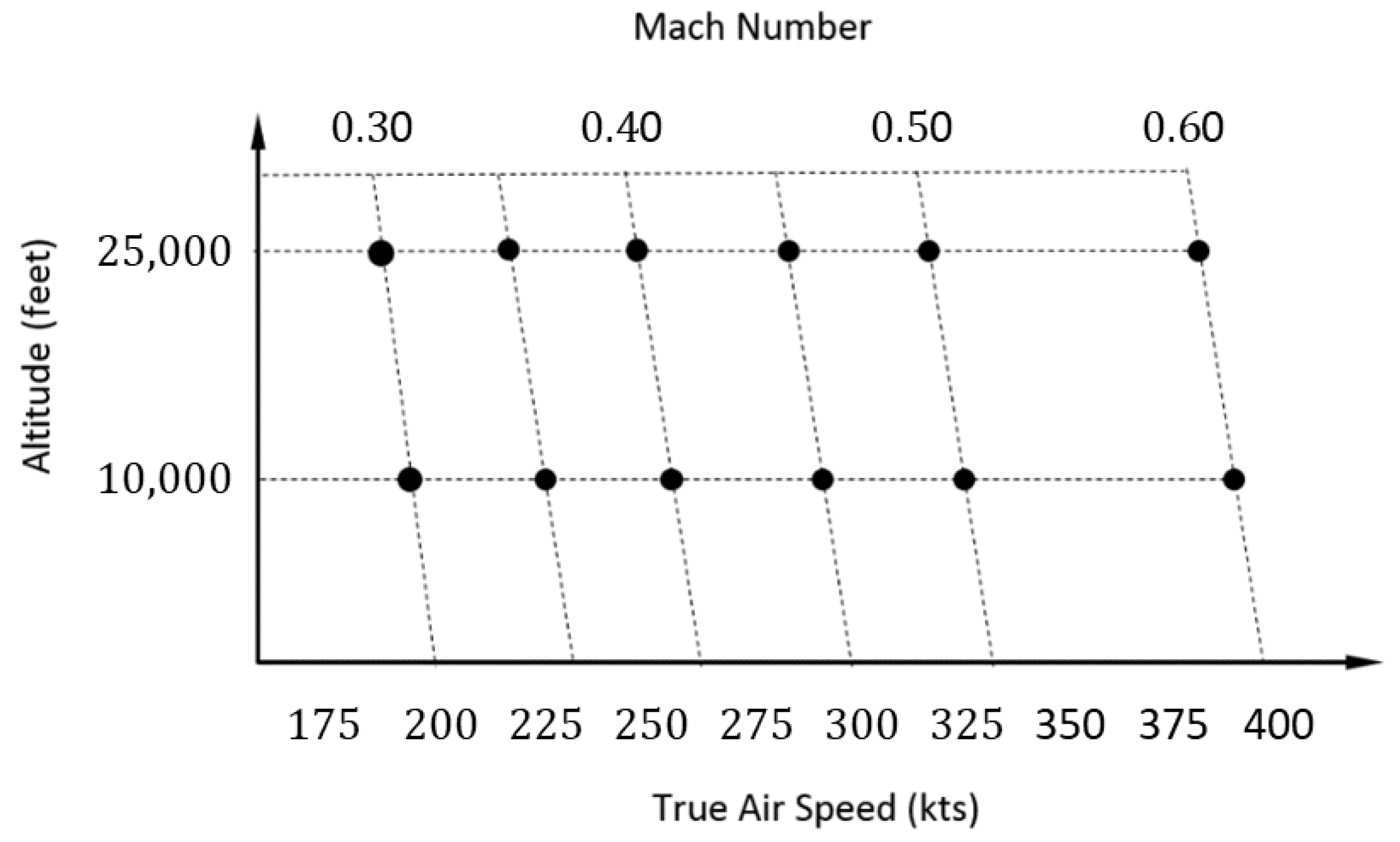
A high-fidelity F-16 simulator based on [21] was used to produce the flight test data. The stability and control derivatives were estimated by the dynamic motion of the aircraft to specific control inputs. There are many manoeuvres to excite dynamic motion around separate axes utilizing individual inputs on each control. The procedures described by Jategaonkar [8] were used as guidelines. It is usually recommended to begin each manoeuvre from a trimmed level flight, to allow about 5 to 10 s of steady flight before applying specific control inputs, and to allow sufficient time after these inputs for the aircraft to oscillate according to the aircraft mode [8]. Trim data for discrete flight conditions expressed in Mach numbers ($M=0.2$ to $0.6$), altitudes ($h=0$ ft to 40,000 ft), and different flight path angles ($\gamma =-5^{\circ }$ to $5^{\circ }$) were collected to develop a preliminary engine thrust model. The system identification manoeuvres were executed at two altitudes and six speed configurations. Note that the F-16 model of [21] is limited to the Mach number range between 0.2 and 0.6. All manoeuvres were started at a level flight trim condition and were not performed at idle or maximum power settings since the aerodynamic coefficients are not affected by the thrust coefficient. The control inputs were configured to execute short-period, phugoid, Dutch roll, and bank-to-bank manoeuvres.

For the aerodynamic model extraction from the test data, control surface deflections, linear accelerations, angular rates, altitude angles, air data, static pressure, engine parameters, and pilot forces were recorded. A sampling frequency of 20–25 Hz was used which usually suffices for a rigid-body aerodynamic model estimation [8,9]. The angle of attack range spanned by the longitudinal manoeuvres was $0^{\circ }$ to ${18}^{\circ }$. Similarly, the angle of attack and angle of sideslip ranges spanned by the lateral manoeuvres were $4^{\circ }$ to ${13}^{\circ }$ and $-8^{\circ }$ to $8^{\circ }$, respectively. The flight test scope is shown in Figure 1.

2.2.3. Data Preprocessing

Because flight data measurement errors can severely degrade the estimation results [8,33,34], before the model identification, two data preprocessing operations were performed. First, to avoid the parameter estimation errors caused by data noise, a low-pass digital filter, developed by Spencer [8] and based on 15 points, was applied. Second, a flight path reconstruction, also known as a data compatibility check, was performed [8,9]. The goal of the flight path reconstruction is to ensure that flight measurements are kinematically consistent and error-free. Flight data are kinematically consistent if the integrated state variables (e.g., the air data obtained from linear accelerations or the altitude angles obtained from rotational kinematics) agree with direct measurements [35].

There were two main parts to the flight path reconstruction. The first was a state integration (integrating translational dynamics, rotational kinematics, and navigational kinematics), and the second was to apply observer equations for a comparison of estimated (reconstructed) and measured outputs. Some drifts in the estimated and measured outputs suggested introducing time lags, biases, and/or scale factors in the measurement signals (e.g., linear accelerations, angular rates, angle of attack, and angle of sideslip) as well as time-invariant atmospheric wind speeds [8,9,36]. The introduced time lags, biases, and/or scale factors in the measurement signals and time-invariant atmospheric wind speeds were estimated using the output error method. Since the body-fixed axes system was defined with respect to the CM, the measured accelerations and velocity components were transferred from the sensor locations to the CM.

3. Methodology

The methodology developed for the preliminary thrust model from steady-state flight tests and for the parameter estimation using the IEEM are described below.

3.1. Development of the Preliminary Thrust Model from Steady-State Flight Tests

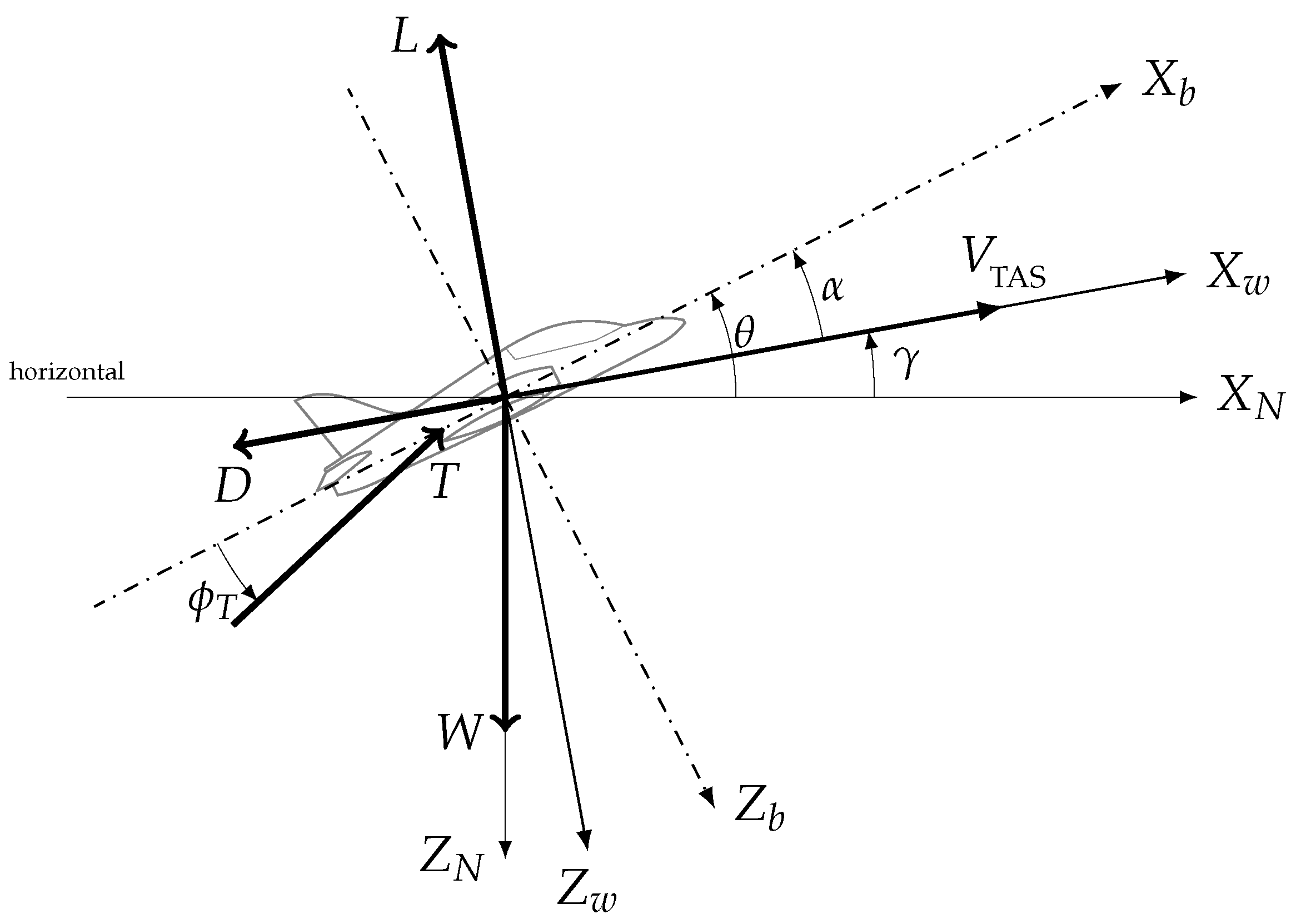
The flight geometry and the applied forces on the air vehicle are shown in Figure 2. The flight path angle $\gamma$ is the angle between the horizontal $X_N$ and the x-wind axis, $X_w$, and $\theta$ is the pitch angle. Summing forces in the $X_w$ and $Z_w$ directions yields:

$$\begin{array}{cc}\hfill \sum F_x& =Tcos(\alpha +{\varphi }_T)-D-Wsin\gamma ,\hfill \end{array}$$

(7)

$$\begin{array}{cc}\hfill \sum F_z& =-Tsin(\alpha +{\varphi }_T)-L+Wcos\gamma ,\hfill \end{array}$$

(8)

where T is the thrust force, D is the drag force, L is the lift force, W is the weight, $\alpha$ is the angle of attack, and ${\varphi }_T$ is the thrust incidence angle. It is assumed that the thrust axis is parallel to the wind axis, i.e., ${\varphi }_T=0$, and that $Tsin\alpha$ is small compared to the weight. Hence, if the aircraft is flying at trim, the sum of the forces must be equal to zero, which leads to the translational equations of motion:

$$\begin{array}{cc}\hfill \sum F_x& =Tcos\alpha -D-Wsin\gamma ,\hfill \end{array}$$

(9)

$$\begin{array}{cc}\hfill \sum F_z& =-L+Wcos\gamma ,\hfill \end{array}$$

(10)

where the drag force, D, and lift force, L, are:

$$\begin{array}{cc}\hfill D& =\overline{q}S{C}_D,\hfill \end{array}$$

(11)

$$\begin{array}{cc}\hfill L& =\overline{q}S{C}_L,\hfill \end{array}$$

(12)

where $\overline{q}$ is the dynamic pressure and S is the reference area.

The relationship between the drag and lift coefficients $C_D$ and $C_L$ is given by [6,21,23]:

$$C_D=C_{D_0}+\frac{1}{\pi e🜇}{C}_L^2=C_{D_0}+K{C}_L^2,$$

(13)

where $C_{D_0}$ is the drag coefficient at a zero angle of attack, e is the Oswald efficiency factor, and 🜇 is the aspect ratio. For swept-wing aircraft, e is assumed to be [37]

$$e=4.61\left(1-0.045\times {🜇}^{0.68}\right){\left(cos{\mathsf{\Lambda }}_{LE}\right)}^{0.15}-3.1({\mathsf{\Lambda }}_{LE}>{30}^{\circ }),$$

(14)

where ${\mathsf{\Lambda }}_{LE}$ is the leading-edge sweep angle. For an F-16 aircraft, $🜇=3$ and ${\mathsf{\Lambda }}_{LE}={40}^{\circ }$, which yields $e=0.9086$. Note that a clean configuration is assumed even though the F16 will often have added equipment. However, this expression is adequate for the preliminary estimation.

During flight, the aircraft weight is known, the angle of attack $\alpha$, flight path angle $\gamma$, and true airspeed $V_{{}_{TAS}}$ are measured, and the air density $\rho$ is calculated using the standard atmosphere model.

In gliding flight, $T\approx 0$ and the sum of forces must be equal to zero, so $\sum F_x=\sum F_z=0$, which leads to:

$$\begin{array}{cc}\hfill 0& =D-Wsin\gamma ,\hfill \end{array}$$

(15)

$$\begin{array}{cc}\hfill 0& =L-Wcos\gamma .\hfill \end{array}$$

(16)

From Equations (11), (12), (15), and (16), we obtain

$$\begin{array}{cc}\hfill C_D& =\frac{Wsin\gamma }{\overline{q}S},\hfill \end{array}$$

(17)

$$\begin{array}{cc}\hfill C_L& =\frac{Wcos\gamma }{\overline{q}S}.\hfill \end{array}$$

(18)

Using Equation (13), $C_{D0}$ is calculated as:

$$C_{D_0}=C_D-\frac{1}{\pi e🜇}{C}_L^2=\frac{Wsin\gamma }{\overline{q}S}-\frac{1}{\pi e🜇}.{\left(\frac{Wcos\gamma }{\overline{q}S}\right)}^2.$$

(19)

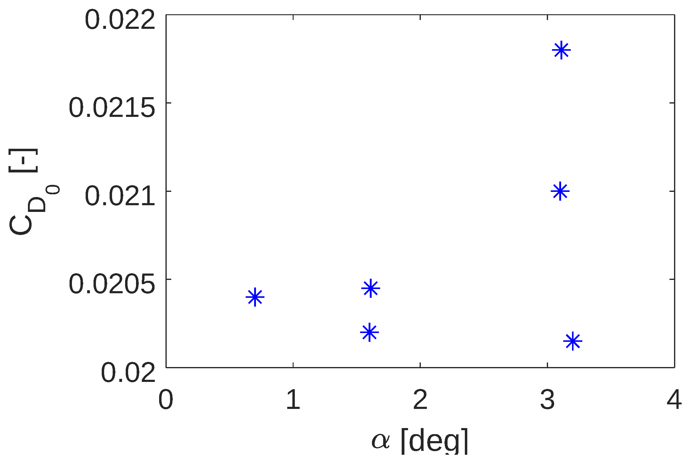
Trim data in gliding flight for different altitudes and speeds were collected, and the results are presented in Figure 3. The averaged $C_{D_0}$ value for the flight is $C_{D_0}=0.0208$, which is very close to the actual value of 0.0202.

Approximate thrust values for each trim point were calculated using the following formulas. The vector-valued function $\overrightarrow{F}$ was constructed using the Newton–Raphson algorithm [23]. Using Equations (9), (10) and (13), the following system equations with two unknowns were obtained:

$$\begin{array}{cc}\hfill F_1& =0=Tcos\alpha -\left(C_{D0}+K{C}_L^2\right)q{S}_{Ref}-Wsin\gamma ,\hfill \end{array}$$

(20)

$$\begin{array}{cc}\hfill F_2& =0=C_{L}q{S}_{Ref}-Wcos\gamma ,\hfill \end{array}$$

(21)

where $\overrightarrow{F}={\left[\begin{array}{cc}{F}_1,& F_2\end{array}\right]}^T$ and $\overrightarrow{\mathsf{\Theta }}={\left[\begin{array}{cc}T,& C_L\end{array}\right]}^T$. After calculating the approximate thrust values for different altitudes, airspeeds, and throttle levers using Equation (15), a preliminary engine propulsion (thrust) model was obtained using Equation (6). The order of the polynomials for throttle position $\left(m\right)$ and Mach number (n) were set as 2 and 3, respectively.

3.2. Parameter Estimation

The mathematical model of the dynamic system (process) in a nonlinear state space form is given by the system:

$$\begin{array}{cc}\hfill \dot{\overrightarrow{x}}\left(t\right)& =f\left[\overrightarrow{x}\left(t\right),\overrightarrow{u}\left(t\right),\overrightarrow{\mathsf{\Theta }}\right],x\left(t_0\right)=x_0,\hfill \end{array}$$

(22)

$$\begin{array}{cc}\hfill \overrightarrow{y}\left(t\right)& =g\left[\overrightarrow{x}\left(t\right),\overrightarrow{u}\left(t\right),\overrightarrow{\mathsf{\Theta }}\right],\hfill \end{array}$$

(23)

where $\overrightarrow{x}\in {\mathbb{R}}^{n_x}$ is the vector of state variables, $\overrightarrow{u}\in {\mathbb{R}}^{n_u}$ is the control input vector, $\overrightarrow{y}\in {\mathbb{R}}^{n_y}$ the system output vector, $\overrightarrow{\mathsf{\Theta }}\in {\mathbb{R}}^{n_q}$ is the unknown parameter vector, $n_u$, $n_x$, $n_q$, and $n_y$ are the system dimensions, and $f:{\mathbb{R}}^{n_x+n_u+n_q}\to {\mathbb{R}}^{n_x}$, $g:{\mathbb{R}}^{n_x+n_u+n_q}\to {\mathbb{R}}^{n_y}$ are general nonlinear functions. Furthermore, the output y is measured periodically and so the measured output is given by

$$\overrightarrow{z}\left(t_k\right)=\overrightarrow{y}\left(t_k\right)+G\overrightarrow{v}\left(t_k\right),k=1,\dots ,N,$$

(24)

where $\overrightarrow{z}\in {\mathbb{R}}^{n_y}$ is the system measurement vector, $\overrightarrow{v}\in {\mathbb{R}}^{n_v}$ is the measurement noise vector, $G\in {\mathbb{R}}^{n_y\times n_v}$ is the additive measurement noise distribution matrix, $n_v$ is the measurement noise dimension, and k is the discrete-time index.

The objective (cost) function J can be calculated from the difference between the measured and estimated responses:

$$J\left(\overrightarrow{\mathsf{\Theta }}\right)=\frac{1}{2}\sum _{k=1}^N{\left(\overrightarrow{z}\left(t_k\right)-\overrightarrow{y}\left(t_k\right)\right)}^T\left(\overrightarrow{z}\left(t_k\right)-\overrightarrow{y}\left(t_k\right)\right).$$

(25)

The unknown coefficient values can be determined using any minimization method. The Gauss–Newton method is one of the most widely used minimization algorithms and was selected for this study. The parameter estimation process is frequently unstable, i.e., a small change in measurement might result in a significant change in the estimated model. Inverse problems that develop because of this scenario are referred to as ill-conditioned problems. Regularization is the process of enhancing the stability of the inversion process by introducing extra constraints that bias the result. The Tikhonov regularization is the most often used approach for regularization. Another possibility is to employ the bounds’ constraint technique. There are lower and upper bounds for the model parameters [38]. To account for simple lower and upper limits on the estimated parameters, the unconstrained optimization problem may be modified to include them. This leads to a linearly constrained optimization problem, formulated as [39]:

$$\underset{\overrightarrow{\mathsf{\Theta }}}{min}J\left(\overrightarrow{\mathsf{\Theta }}\right)\mathrm{subject}\mathrm{to}{\overrightarrow{\mathsf{\Theta }}}_{min}\le \overrightarrow{\mathsf{\Theta }}\le {\overrightarrow{\mathsf{\Theta }}}_{max},$$

(26)

which, in standard form, is

$$\underset{\overrightarrow{\mathsf{\Theta }}}{min}J\left(\overrightarrow{\mathsf{\Theta }}\right)\mathrm{subject}\mathrm{to}{c}_1:\overrightarrow{\mathsf{\Theta }}-{\overrightarrow{\mathsf{\Theta }}}_{min}\ge 0,c_2:{\overrightarrow{\mathsf{\Theta }}}_{max}-\overrightarrow{\mathsf{\Theta }}\ge 0.$$

(27)

Barrier methods [40] offer an elegant approach to this constrained optimization problem. The constrained optimization problem is recast as an unconstrained problem in which the objective function is extended with logarithmic barrier terms. The unconstrained problem (combined objective/barrier function) is given by

$$\underset{\overrightarrow{\mathsf{\Theta }}}{min}P\left(\overrightarrow{\mathsf{\Theta }};\mu \right)=\underset{\overrightarrow{\mathsf{\Theta }}}{min}J\left(\overrightarrow{\mathsf{\Theta }}\right)-\mu \left[log\left(\overrightarrow{\mathsf{\Theta }}-{\overrightarrow{\mathsf{\Theta }}}_{min}\right)+log\left({\overrightarrow{\mathsf{\Theta }}}_{max}-\overrightarrow{\mathsf{\Theta }}\right)\right].$$

(28)

3.3. Equation Error Method (EEM)

The EEM is used to determine nonstate parameters such as force and moment coefficients, which are not integrated during simulation. By using the equation error form, there is no need to integrate the equations of motion to achieve model outputs since the matching is performed in the equations of motion (hence the term “equation error” [14]). Furthermore, by minimizing the differences in the least-square sense between measured and model (estimated) responses, the equation error approach estimates the unknown parameter vector (aerodynamic stability and control derivatives).

A wide range of information is needed to derive total aerodynamic force and moment coefficients from flight data, such as the angular rates and accelerations, linear accelerations, thrust-induced forces and moments on the body axis, dynamic pressure, and aircraft mass and inertia data. The location of the accelerometer and air data system is often used to transfer air data and accelerations to the CM. In addition, for each manoeuvre, the centre of gravity location must be determined to transfer total moments to the aerodynamic moment centre (MC) around which an aerodynamic model can be constructed. The coefficients of the nondimensional force and moment are obtained by substituting measured and known quantities. The EEM is used to model the functional dependence of aerodynamic forces and moments on aircraft motion and control variables since propulsive forces and moments are generally obtained from ground tests. The process is illustrated in Figure 4.

The engine model was based on static thrust look-up tables derived from data provided by the engine manufacturer. Engine dynamics were modelled by applying lag filters to the static engine model. Throughout each manoeuvre, the throttles were held in the trim position.

A preprocessing step was required for the aerodynamic forces and moments since they were not directly measured but could be obtained from the measurements of the related variables, linear accelerations, angular rates, mass properties, and other external forces and moments, as shown in Figure 4.

The computation of the nondimensional force and moment coefficients were performed using the following equations. The body-fixed specific accelerations at the CM were computed from measured accelerations at the accelerometer sensor position using the following transformation:

$$\begin{array}{cc}\hfill a_{s_x}& =a_{s_x}^{AS}+(q^2+r^2)x_{AS/B}-(pq-\dot{r})y_{AS/B}-(pr+\dot{q})z_{AS/B},\hfill \end{array}$$

(29)

$$\begin{array}{cc}\hfill a_{s_y}& =a_{s_y}^{AS}-(pq+\dot{r})x_{AS/B}+(p^2+r^2)y_{AS/B}-(qr-\dot{p})z_{AS/B},\hfill \end{array}$$

(30)

$$\begin{array}{cc}\hfill a_{s_z}& =a_{s_z}^{AS}-(pr-\dot{q})x_{AS/B}-(qr+\dot{p})y_{AS/B}+(p^2+q^2)z_{AS/B}.\hfill \end{array}$$

(31)

Having obtained the specific linear accelerations at the CM, the body-axes aerodynamic force coefficients were obtained as

$$\left[\begin{array}{c}{C}_X\\ C_Y\\ C_Z\end{array}\right]=\frac{1}{\overline{q}S}m\left[\begin{array}{c}{a}_{s_x}\\ a_{s_y}\\ a_{s_z}\end{array}\right]-\left[\begin{array}{c}T\\ 0\\ 0\end{array}\right].$$

(32)

The nondimensional force components resolved in the wind axis can be obtained using the transformation matrix and written as:

$$\left[\begin{array}{c}-C_D\\ -C_C\\ -C_L\end{array}\right]=\frac{1}{\overline{q}S}\left[\begin{array}{ccc}cos\alpha cos\beta & sin\beta & sin\alpha cos\beta \\ -cos\alpha sin\beta & cos\beta & -sin\alpha sin\beta \\ -sin\alpha & 0& cos\alpha \end{array}\right]\left[\begin{array}{c}m{a}_{s_x}-T\\ m{a}_{s_y}\\ m{a}_{s_z}\end{array}\right].$$

(33)

The aerodynamic body-axes’ moments at the CM were computed as

$$\left[\begin{array}{c}{l}_a\\ m_a\\ n_a\end{array}\right]=\left[\begin{array}{c}p\\ q\\ r\end{array}\right]\times \left[\begin{array}{ccc}{I}_{XX}& -I_{XY}& -I_{XZ}\\ -I_{XY}& I_{YY}& -I_{YZ}\\ -I_{XZ}& -I_{YZ}& I_{ZZ}\end{array}\right]\left[\begin{array}{c}p\\ q\\ r\end{array}\right]+\left[\begin{array}{ccc}{I}_{XX}& -I_{XY}& -I_{XZ}\\ -I_{XY}& I_{YY}& -I_{YZ}\\ -I_{XZ}& -I_{YZ}& I_{ZZ}\end{array}\right]\left[\begin{array}{c}\dot{p}\\ \dot{q}\\ \dot{r}\end{array}\right].$$

(34)

The body-axes’ rolling, pitching, and yawing coefficients referred to CM were obtained from:

$$\left[\begin{array}{c}{C}_l\\ C_m\\ C_n\end{array}\right]=\frac{1}{\overline{q}S}\left[\begin{array}{ccc}1/b& 0& 0\\ 0& 1/\overline{c}& 0\\ 0& 0& 1/b\end{array}\right]\left[\begin{array}{c}{l}_a\\ m_a\\ n_a\end{array}\right].$$

(35)

The moment coefficients referred to MC on the vehicle were obtained from:

$$\begin{array}{cc}\hfill C_l^{MC}& =C_l-C_Z\frac{x_{MC/B}}{b}+C_Y\frac{z_{MC/B}}{b},\hfill \end{array}$$

(36)

$$\begin{array}{cc}\hfill C_m^{MC}& =C_m-C_X\frac{z_{MC/B}}{\overline{c}}+C_Z\frac{x_{MC/B}}{\overline{c}},\hfill \end{array}$$

(37)

$$\begin{array}{cc}\hfill C_n^{MC}& =C_n-C_Y\frac{x_{MC/B}}{b}+C_X\frac{y_{MC/B}}{b}.\hfill \end{array}$$

(38)

For the EEM estimation, the control input, state variables, observation variables, and unknown (estimated) variables are listed in

Table 2. Control input, state variables, and output vectors and unknown variables for the EEM.

Symbol	Description	Variables
$\overrightarrow{u}$	Control input vector	$\left[V,\alpha ,\beta ,p,q,r,{\delta }_{\mathrm{lef}},{\delta }_e,{\delta }_a,{\delta }_r{\delta }_{sb},M\right]$
$\overrightarrow{x}$	State variable vector	[ ]
$\overrightarrow{y}$	Observation vector	$\left[C_D\right]$ or $\left[C_L\right]$
$\overrightarrow{\mathsf{\Theta }}$	Unknown variables	$\left[C_D\right]$ or $\left[C_L\right]$ model parameters

.

Determination and Validation of the Aerodynamic Model Structure

In the process of evaluating the identified model’s correctness, accuracy, and applicability, each coefficient was assigned a unique model structure, which represents a multi-input, single-output subspace. This approach allowed for a greater flexibility and simplified the training task. The initial goal of aerodynamic model development is to determine a good model structure. The model should be as simple as possible while being sufficiently complex to capture the necessary dynamics. Although restricting the number of terms used simplifies computing, it is essential to use the correct terms to ensure a high degree of accuracy. Choosing which terms to include in each coefficient model is a tedious process and is known as “feature selection”.

There are numerous well-known methods for feature selection, including stepwise regression, multivariate orthogonal functions, and generalized additive models. The aerodynamic model structure used in this study was based on that developed by Grauer and Morelli [41]. They developed a generic, precise, and simple nonlinear aerodynamics model using multivariate orthogonal function modelling to investigate measured wind tunnel aerodynamic databases for eight aircraft over a wide range of flight regimes. The most critical modelling terms (the number of selected instances was high) for each coefficient were selected as frozen model terms. The remaining model terms for longitudinal coefficients were selected using a correlation-based stepwise regression method. The algorithm started by generating a set of candidate model terms based on a set of base regressors and a maximum term order. Then, the pairwise correlation among model terms was compared, and some terms were removed. Finally, a binary particle swarm optimization was utilized to generate the best subset of the remaining terms. Certain additions and rejections to the structure of the underlying aerodynamic model were made using the statistical and qualitative graphical findings analysed by Jategaonkar and Thielecke [33] and the resampling methods analysed by Millidere et al. [19].

To evaluate the statistical accuracy of the results, first a check was performed to find out whether the expected value was reasonable. The magnitude should be close to the real value. Next, values of standard deviation, coefficient of variation (COV), and correlation matrix were checked. The COV of any term should not exceed 50% since a significant uncertainty level indicates low information in the derivative estimate. None of the correlations among the two independent terms should exceed 0.95 because the existence of data collinearity compromises the parameter estimation results.

Comparing the time histories of flight-measured and model-estimated responses is a widespread method for the qualitative evaluation of the model’s fidelity. Some inconsistencies in matching the two responses often offer critical information for improving the model fidelity. The residuals test (the difference between the predicted and measured response), also known as cross-plots of residuals, is a good indicator of the reliability of the assumptions made about measurement noise on the system. Ideally, the residual distribution should be flat and centred near zero.

Rather than evaluating the model on the training data, the trained model was evaluated for the data in the testing dataset not used in the training model. The k-fold cross-validation method was used as the resampling method.

3.4. Iterative Equation Error Method (IEEM)

When the thrust force is known, the EEM is used to find the aerodynamic force and moment coefficients. However, when thrust data are not available, thrust is calculated using the assumptions from steady-state flight tests, and a preliminary simplified turbofan engine thrust model is developed. A good preliminary design is needed as a starting point for all optimization-based design methods. Otherwise, there is no guarantee that the search engine will find a satisfactory solution. The preliminary design is usually accomplished by applying classical methods and employing the IEEM. Since the thrust force does not produce any moment and the angle of sideslip is relatively small in longitudinal manoeuvres, the problem is reduced to identifying aerodynamic drag and lift force coefficients.

The IEEM consists of a starting point and then using a systematic method to obtain a refined estimate of the solution. In the end, it is expected to obtain a solution that simultaneously satisfies the given output vector. The process starts by choosing a reasonable starting point for an unknown parameter vector ${\overrightarrow{\mathsf{\Theta }}}^{\left(0\right)}$. If the starting point is far from the optimum, estimations may not lead to a converged solution. The unknown parameter vector is split into two sub-vectors, ${\overrightarrow{\mathsf{\Theta }}}_F$ and ${\overrightarrow{\mathsf{\Theta }}}_E$. Vector ${\overrightarrow{\mathsf{\Theta }}}_F$ contains the fixed coefficients, and ${\overrightarrow{\mathsf{\Theta }}}_E$ contains the parameters to be estimated. The starting point can be substituted into the cost function, which can be used to calculate a new estimate for $C_D$ coefficient parameters. The fixed parameters, the new estimates of the $C_D$ coefficient parameters along with the previous estimates for $C_T$ are then substituted into the cost function to compute a new estimate for the $C_L$ coefficient parameters. This process is repeated to calculate a new estimate for the $C_T$ coefficient. Then, the entire procedure is repeated until the relative error, ${\epsilon }_a$ falls below a prespecified stopping criterion, ${\epsilon }_s$, or until the maximum number of iterations is reached.

For the IEEM estimation, the control input, state variables, measured/model output vectors, and unknown (estimated) variables are listed in

Table 3. Control input, state variables, and output vectors and unknown variables for the IEEM.

Symbol	Description	Variables
$\overrightarrow{u}$	Control input vector	$\left[V,\alpha ,\beta ,p,q,r,{\delta }_{lef},{\delta }_e,{\delta }_a,{\delta }_r,{\delta }_{sb},M\right]$
$\overrightarrow{x}$	State variable vector	[ ]
$\overrightarrow{y}$	Observer vector	$\left[a_{s_X},a_{s_Z}\right]$
$\overrightarrow{\mathsf{\Theta }}$	Unknown variables	$\left[C_D,C_L,C_T\right]$ Model parameters

.

The equations that describe the IEEM can be expressed as:

$$\frac{1}{m}\overline{q}S{\left[\begin{array}{ccc}cos\alpha cos\beta & sin\beta & sin\alpha cos\beta \\ -cos\alpha sin\beta & cos\beta & -sin\alpha sin\beta \\ -sin\alpha & 0& cos\alpha \end{array}\right]}^T\left[\begin{array}{c}-C_D\\ -C_C\\ -C_L\end{array}\right]+\frac{1}{m}\left[\begin{array}{c}T\\ 0\\ 0\end{array}\right]=\left[\begin{array}{c}{a}_{s_x}\\ a_{s_y}\\ a_{s_z}\end{array}\right].$$

(39)

By inserting Equation (4) into Equation (39), we obtain

$$\frac{1}{m}\overline{q}S{\left[\begin{array}{ccc}cos\alpha cos\beta & sin\beta & sin\alpha cos\beta \\ -cos\alpha sin\beta & cos\beta & -sin\alpha sin\beta \\ -sin\alpha & 0& cos\alpha \end{array}\right]}^T\left[\begin{array}{c}-C_D\\ -C_C\\ -C_L\end{array}\right]+\frac{1}{m}\left[\begin{array}{c}{T}_0\overline{\sigma }{C}_T\\ 0\\ 0\end{array}\right]=\left[\begin{array}{c}{a}_{s_x}\\ a_{s_y}\\ a_{s_z}\end{array}\right].$$

(40)

To eliminate the sideslip dependency, only longitudinal manoeuvres are employed, where it is assumed that $\beta \approx C_C\approx 0$, so that Equation (40) becomes:

$$\frac{1}{m}\overline{q}S\left[\begin{array}{cc}cos\alpha & -sin\alpha \\ sin\alpha & cos\alpha \end{array}\right]\left[\begin{array}{c}-C_D\\ -C_L\end{array}\right]+\frac{1}{m}\left[\begin{array}{c}{T}_0\overline{\sigma }{C}_T\\ 0\end{array}\right]=\left[\begin{array}{c}{a}_{s_x}\\ a_{s_z}\end{array}\right].$$

(41)

4. Application and Results

4.1. Developed Simplified Turbofan Thrust Model

Numerous flight tests were conducted for different flight conditions expressed in Mach numbers ($M=0.2$ to $M=0.6$), altitudes ($h=0$ ft. to $h=$ 40,000 ft.), and different flight path angles ($\gamma =-5^{\circ }$ to $\gamma =5^{\circ }$). A simplified turbofan thrust model was obtained using:

$$C_T(h,M,{\delta }_{TLA})=\frac{T(h,M,{\delta }_{TLA})}{\frac{\rho \left(h\right)}{{\rho }_0}{T}_0{\left[1+\frac{1}{2}(\gamma -1)M^{{}^2}\right]}^{1/(\gamma -1)}}=\sum _{i=0}^n\sum _{j=0}^m{C}_{T_{ij}}\left(h\right)M^i{\delta }_{TLA}^j.$$

(42)

To determine which m and n values generate the best fit, the mean square errors were compared using a k-fold cross validation [27] for different n and m values. For $n=3$ and $m=2$, the best overall result was obtained.

The comparisons of trim-constructed and estimated nondimensional thrust coefficients for different altitudes are shown in Figure 5. It is observed that the estimated results are compatible with the constructed results from trim values.

4.2. Application of the IEEM

After the engine thrust model was developed, the IEEM was used to obtain a reasonable starting point for longitudinal aerodynamic coefficients. For the IEEM, the developed model structures for the drag and lift coefficients, $C_D$ and $C_L$, were:

$$\begin{array}{c}{C}_D=C_{D_0}+\left[C_{D_{\alpha }}·\alpha +C_{D_{{\alpha }^2}}·{\alpha }^2+C_{D_{{\alpha }^3}}·{\alpha }^3\right]+\left[C_{D_{{\delta }_e}}·{\delta }_e+C_{D_{{\delta }_e\alpha }}·{\delta }_e·\alpha +C_{D_{{\delta }_e{\alpha }^2}}·{\delta }_e·{\alpha }^2\right]+\left[C_{D_q}·\frac{qc}{2V}+C_{D_{q\alpha }}·\frac{qc}{2V}·\alpha \right]\hfill \\ \hspace{1em}\hspace{1em}\hspace{1em}\hspace{1em}\hspace{1em}\hspace{1em}\hspace{1em}\hspace{1em}\hspace{1em}\hspace{1em}\hspace{1em}\hspace{1em}\hspace{1em}\hspace{1em}+\left[C_{D_{{\delta }_{lef}}}·{\delta }_{lef}+C_{D_{{\delta }_{lef}\alpha }}·{\delta }_{lef}·\alpha +C_{D_{{\delta }_{lef}{\alpha }_{10}^1}}·{\delta }_{lef}·{\left(\alpha -{\alpha }_{{10}^{\circ }}\right)}_{{}_{+}}{C}_{D_{{\delta }_{lef}{\alpha }_{15}^1}}·{\delta }_{lef}·{\left(\alpha -{\alpha }_{{15}^{\circ }}\right)}_{{}_{+}}\right],\hfill \end{array}$$

(43)

$$\begin{array}{c}{C}_L=\left[C_{L_0}+C_{L_{\alpha }}·\alpha +C_{L_{{\alpha }_5^1}}·{\left(\alpha -{\alpha }_{5^{\circ }}\right)}_{{}_{+}}+C_{L_{{\alpha }_{10}^1}}·{\left(\alpha -{\alpha }_{{10}^{\circ }}\right)}_{{}_{+}}+C_{L_{{\alpha }_{15}^1}}·{\left(\alpha -{\alpha }_{{15}^{\circ }}\right)}_{{}_{+}}\right]\hfill \\ \hspace{1em}\hspace{1em}\hspace{1em}+\left[C_{L_{{\delta }_e}}·{\delta }_e+C_{L_{{\delta }_e\alpha }}·{\delta }_e·\alpha +C_{L_{{\delta }_e{\alpha }^2}}·{\delta }_e·{\alpha }^2\right]+\left[C_{L_q}·\frac{qc}{2V}+C_{L_{q\alpha }}·\frac{qc}{2V}·\alpha \right]+\left[C_{L_{{\delta }_{lef}}}·{\delta }_{lef}+C_{L_{{\delta }_{lef}\alpha }}·{\delta }_{lef}·\alpha \right.\\ \hfill \left.\hspace{1em}\hspace{1em}\hspace{1em}\hspace{1em}\hspace{1em}\hspace{1em}\hspace{1em}\hspace{1em}\hspace{1em}\hspace{1em}+C_{L_{{\delta }_{lef}{\alpha }_5^1}}·{\delta }_{lef}·{\left(\alpha -{\alpha }_{5^{\circ }}\right)}_{{}_{+}}+C_{L_{{\delta }_{lef}{\alpha }_{10}^1}}·{\delta }_{lef}·{\left(\alpha -{\alpha }_{{10}^{\circ }}\right)}_{{}_{+}}{C}_{L_{{\delta }_{lef}{\alpha }_{15}^1}}·{\delta }_{lef}·{\left(\alpha -{\alpha }_{{15}^{\circ }}\right)}_{{}_{+}}+C_{L_{{\delta }_{lef}q\alpha }}·{\delta }_{lef}·q·\alpha \right].\end{array}$$

(44)

The parameter estimates of $C_D$ and $C_L$ are tabulated in

Table 4. The estimates, standard deviations, and COVs of the parameters of coefficient $C_D$.

Index	Parameter	Estimate	Std. Dev.	COV
1	$C_{D_0}$	$0.0202$	$7.11\times {10}^{-05}$	0.35
2	$C_{D_{\alpha }}$	$-0.0860$	$3.72\times {10}^{-03}$	4.33
3	$C_{D_{{\alpha }^2}}$	$4.26$	$2.67\times {10}^{-02}$	0.63
4	$C_{D_{{\alpha }^3}}$	$-0.383$	$2.49\times {10}^{-02}$	6.50
5	$C_{D_{{\delta }_e}}$	$-0.0640$	$2.53\times {10}^{-03}$	3.95
6	$C_{D_{{\delta }_e\alpha }}$	$0.357$	$6.73\times {10}^{-03}$	1.88
7	$C_{D_{{\delta }_e{\alpha }^2}}$	$1.87$	$8.23\times {10}^{-03}$	0.44
8	$C_{D_q}$	$-0.366$	$2.51\times {10}^{-02}$	6.86
9	$C_{D_{q\alpha }}$	$20.2$	$2.73\times {10}^{-01}$	1.35
10	$C_{D_{{\delta }_{lef}}}$	$0.0440$	$1.91\times {10}^{-03}$	4.34
11	$C_{D_{{\delta }_{lef}\alpha }}$	$-1.00$	$1.57\times {10}^{-02}$	1.57
12	$C_{D_{{\delta }_{lef}{\alpha }_{10}^1}}$	$-0.164$	$2.49\times {10}^{-03}$	1.52
13	$C_{D_{{\delta }_{lef}{\alpha }_{15}^1}}$	$0.639$	$3.38\times {10}^{-03}$	0.52

and

Table 5. The estimates, standard deviations, and COVs of the parameters of coefficient $C_L$.

Index	Parameter	Estimate	Std. Dev.	COV
1	$C_{L_0}$	0.0999	$9.54\times {10}^{-05}$	0.09
2	$C_{L_{\alpha }}$	3.74	$2.25\times {10}^{-03}$	0.06
3	$C_{L_{{\alpha }_5^1}}$	0.149	$2.12\times {10}^{-03}$	1.42
4	$C_{L_{{\alpha }_{10}^1}}$	0.137	$6.17\times {10}^{-03}$	4.50
5	$C_{L_{{\alpha }_{15}^1}}$	−1.93	$4.15\times {10}^{-02}$	2.15
6	$C_{L_{{\delta }_e}}$	0.510	$3.15\times {10}^{-03}$	0.62
7	$C_{L_{{\delta }_e\alpha }}$	−0.0840	$1.75\times {10}^{-02}$	20.53
8	$C_{L_{{\delta }_e{\alpha }^2}}$	6.62	$1.05\times {10}^{-01}$	1.58
9	$C_{L_q}$	29.1	$2.20\times {10}^{-02}$	0.08
10	$C_{L_{q\alpha }}$	20.9	$3.80\times {10}^{-02}$	0.18
11	$C_{L_{{\delta }_{lef}}}$	−0.178	$1.15\times {10}^{-03}$	0.64
12	$C_{L_{{\delta }_{lef}\alpha }}$	0.505	$2.05\times {10}^{-02}$	4.06
13	$C_{L_{{\delta }_{lef}{\alpha }_5^1}}$	0.516	$1.72\times {10}^{-02}$	3.33
14	$C_{L_{{\delta }_{lef}{\alpha }_{10}^1}}$	−0.893	$1.15\times {10}^{-02}$	1.28
15	$C_{L_{{\delta }_{lef}{\alpha }_{15}^1}}$	3.46	$1.25\times {10}^{-01}$	3.61
16	$C_{L_{{\delta }_{lef}q\alpha }}$	−54.5	$2.01\times {10}^{-02}$	0.04

, respectively. The COV for each coefficient was below 50% indicating a very low estimate uncertainty.

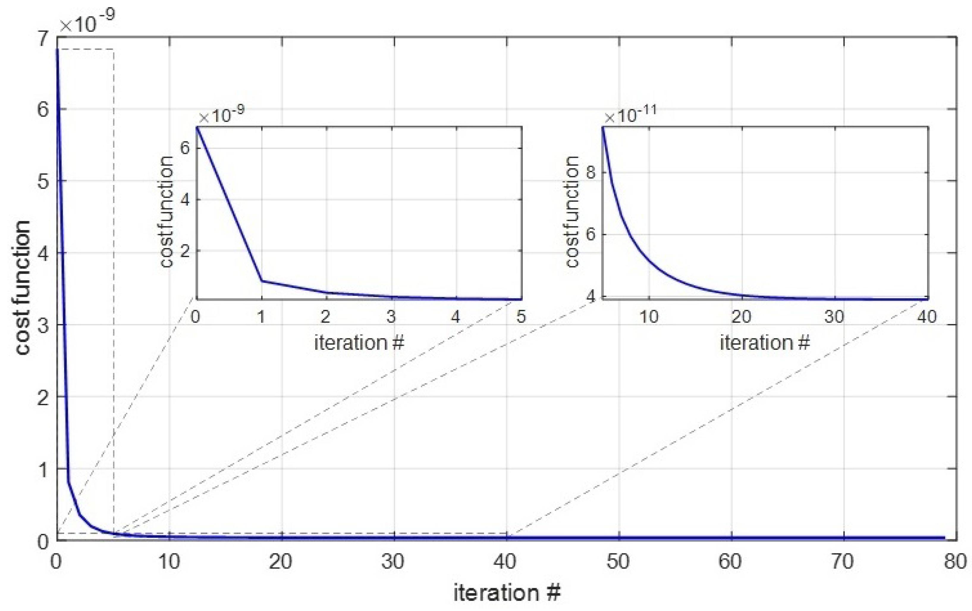
Figure 6 shows the cost function’s convergence during the application of the IEEM. The cost function decreases dramatically in the first 5 iterations and converges to a small steady-state value approximately at the 40th iteration. Hence, the maximum number of iterations was set to 40 to obtain good results.

Table 6. $C_D$ coefficient parameter estimates and errors.

k	${\mathit{C}}_{{\mathit{D}}_0}$	${\mathit{C}}_{{\mathit{D}}_{\mathit{\alpha }}}$	${\mathit{C}}_{{\mathit{D}}_{{\mathit{\alpha }}^2}}$	${\mathit{C}}_{{\mathit{D}}_{{\mathit{\alpha }}^3}}$	${\mathit{C}}_{{\mathit{D}}_{{\mathit{\delta }}_{\mathit{e}}}}$	${\mathit{C}}_{{\mathit{D}}_{{\mathit{\delta }}_{\mathit{e}}\mathit{\alpha }}}$	${\mathit{C}}_{{\mathit{D}}_{{\mathit{\delta }}_{\mathit{e}}{\mathit{\alpha }}^2}}$
1	0.0206	0.057	2.458	0.027	−0.010	−0.675	5.277
2	0.0206	0.049	2.581	0.168	−0.038	−0.373	4.673
3	0.0201	0.032	3.180	−0.764	−0.053	0.218	1.957
4	0.0200	0.009	3.558	−1.086	−0.059	0.353	1.315
5	0.0200	−0.011	3.780	−1.074	−0.060	0.347	1.370
10	0.0202	−0.061	4.173	−0.675	−0.061	0.320	1.702
15	0.0202	−0.074	4.237	−0.531	−0.062	0.332	1.780
20	0.0202	−0.079	4.250	−0.466	−0.063	0.343	1.818
30	0.0202	−0.083	4.256	−0.413	−0.063	0.353	1.849
40	0.0202	−0.085	4.256	−0.395	−0.064	0.357	1.859
50	0.0202	−0.085	4.254	−0.389	−0.064	0.357	1.863
80	0.0202	−0.086	4.258	−0.383	−0.064	0.357	1.868
Actual	0.0209	−0.1411	4.311	−0.273	−0.057	0.205	2.442

,

Table 7. $C_D$ coefficient parameter estimates and estimation error—continued.

k	${\mathit{C}}_{{\mathit{D}}_{\mathit{q}}}$	${\mathit{C}}_{{\mathit{D}}_{\mathit{q}\mathit{\alpha }}}$	${\mathit{C}}_{{\mathit{D}}_{{\mathit{\delta }}_{\mathbf{lef}}}}$	${\mathit{C}}_{{\mathit{D}}_{{\mathit{\delta }}_{\mathbf{lef}}\mathit{\alpha }}}$	${\mathit{C}}_{{\mathit{D}}_{{\mathit{\delta }}_{\mathbf{lef}}{\mathit{\alpha }}_{10}^1}}$	${\mathit{C}}_{{\mathit{D}}_{{\mathit{\delta }}_{\mathbf{lef}}{\mathit{\alpha }}_{15}^1}}$	$\mathit{\delta }\left(\%\right)$
1	0.534	22.497	−0.088	0.357	−0.337	0.700	74.242
2	0.564	21.120	−0.080	0.259	−0.368	0.674	62.844
3	0.122	18.320	−0.057	−0.097	−0.243	0.635	32.398
4	−0.030	16.393	−0.037	−0.353	−0.159	0.625	34.181
5	−0.097	15.841	−0.020	−0.530	−0.121	0.627	30.293
10	−0.205	17.114	0.022	−0.897	−0.114	0.620	17.260
15	−0.267	18.354	0.033	−0.969	−0.134	0.625	14.387
20	−0.309	19.142	0.038	−0.989	−0.147	0.631	13.246
30	−0.348	19.870	0.042	−1.002	−0.159	0.637	12.432
40	−0.360	20.107	0.043	−1.005	−0.163	0.639	12.191
50	−0.364	20.184	0.044	−1.005	−0.164	0.640	12.097
80	−0.366	20.217	0.044	−1.002	−0.164	0.639	11.987
Actual	−0.234	19.579	0.0833	−1.067	−0.146	0.636

,

Table 8. $C_L$ coefficient parameter estimates and errors.

k	${\mathit{C}}_{{\mathit{L}}_0}$	${\mathit{C}}_{{\mathit{L}}_{\mathit{\alpha }}}$	${\mathit{C}}_{{\mathit{L}}_{{\mathit{\alpha }}_5^1}}$	${\mathit{C}}_{{\mathit{L}}_{{\mathit{\alpha }}_{10}^1}}$	${\mathit{C}}_{{\mathit{L}}_{{\mathit{\alpha }}_{15}^1}}$	${\mathit{C}}_{{\mathit{L}}_{{\mathit{\delta }}_{\mathit{e}}}}$	${\mathit{C}}_{{\mathit{L}}_{{\mathit{\delta }}_{\mathit{e}}\mathit{\alpha }}}$	${\mathit{C}}_{{\mathit{L}}_{{\mathit{\delta }}_{\mathit{e}}{\mathit{\alpha }}^2}}$	${\mathit{C}}_{{\mathit{L}}_{\mathit{q}}}$
1	0.0992	3.747	0.175	0.114	−1.834	0.477	−0.084	3.788	28.742
2	0.0998	3.740	0.162	0.145	−1.984	0.505	−0.706	6.144	28.985
3	0.0998	3.737	0.156	0.137	−1.982	0.508	−0.804	6.615	29.016
4	0.0999	3.736	0.152	0.135	−1.981	0.509	−0.833	6.750	29.043
5	0.0999	3.735	0.151	0.136	−1.976	0.510	−0.838	6.758	29.064
10	0.0999	3.735	0.149	0.140	−1.953	0.510	−0.844	6.722	29.110
15	0.0999	3.736	0.149	0.139	−1.942	0.510	−0.843	6.687	29.115
20	0.0999	3.736	0.149	0.139	−1.936	0.510	−0.840	6.660	29.114
30	0.0999	3.736	0.149	0.138	−1.932	0.510	−0.838	6.635	29.112
40	0.0999	3.736	0.149	0.137	−1.931	0.510	−0.837	6.627	29.110
50	0.0999	3.736	0.149	0.137	−1.931	0.510	−0.836	6.624	29.109
80	0.0999	3.737	0.149	0.137	−1.931	0.510	−0.835	6.620	29.107
Actual	0.0995	3.737	0.156	0.135	−1.907	0.489	−0.612	4.808	29.136

and

Table 9. $C_L$ coefficient parameter estimates and errors—continued.

k	${\mathit{C}}_{{\mathit{L}}_{\mathit{q}\mathit{\alpha }}}$	${\mathit{C}}_{{\mathit{L}}_{{\mathit{\delta }}_{\mathbf{lef}}}}$	${\mathit{C}}_{{\mathit{L}}_{{\mathit{\delta }}_{\mathbf{lef}}\mathit{\alpha }}}$	${\mathit{C}}_{{\mathit{L}}_{{\mathit{\delta }}_{\mathbf{lef}}{\mathit{\alpha }}_5^1}}$	${\mathit{C}}_{{\mathit{L}}_{{\mathit{\delta }}_{\mathbf{lef}}{\mathit{\alpha }}_{10}^1}}$	${\mathit{C}}_{{\mathit{L}}_{{\mathit{\delta }}_{\mathbf{lef}}{\mathit{\alpha }}_{15}^1}}$	${\mathit{C}}_{{\mathit{L}}_{{\mathit{\delta }}_{\mathbf{lef}}\mathit{q}\mathit{\alpha }}}$	$\mathit{\delta }\left(\%\right)$
1	28.348	−0.175	0.511	0.345	−0.804	3.150	−74.932	23.474
2	21.385	−0.178	0.507	0.430	−0.862	3.620	−54.764	12.770
3	21.424	−0.178	0.508	0.473	−0.860	3.625	−52.506	12.316
4	21.258	−0.178	0.508	0.494	−0.870	3.624	−51.168	11.905
5	21.087	−0.178	0.508	0.504	−0.882	3.609	−50.866	10.577
10	20.619	−0.178	0.508	0.515	−0.903	3.550	−51.594	10.412
15	20.640	−0.178	0.507	0.516	−0.902	3.519	−52.577	9.521
20	20.736	−0.178	0.506	0.516	−0.899	3.501	−53.345	8.487
30	20.852	−0.178	0.505	0.516	−0.895	3.489	−54.101	8.134
40	20.899	−0.178	0.505	0.516	−0.894	3.486	−54.359	8.004
50	20.921	−0.178	0.505	0.516	−0.893	3.485	−54.452	7.892
80	20.954	−0.178	0.505	0.516	−0.893	3.485	−54.528	7.812
Actual	22.597	−0.178	0.511	0.454	−0.912	3.361	−59.489

list the calculated parameter estimates and the associated estimation errors for the drag and lift coefficients. The estimation error was calculated from $\delta =\parallel {\overrightarrow{\mathsf{\Theta }}}^k-{\overrightarrow{\mathsf{\Theta }}}^{\mathrm{actual}}\parallel /\parallel {\overrightarrow{\mathsf{\Theta }}}^{\mathrm{actual}}\parallel$.

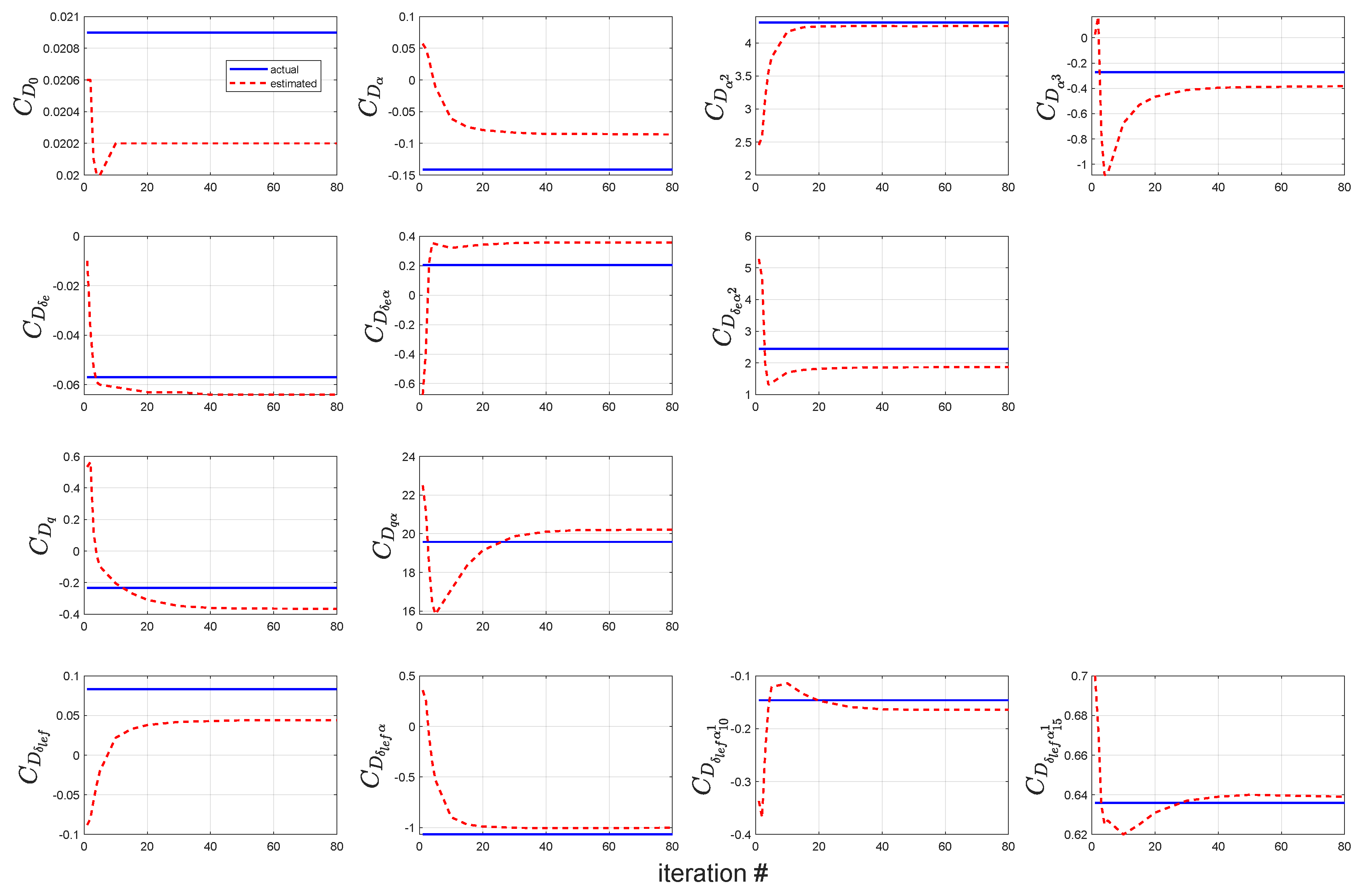
Figure 7 shows the variation in the estimated parameters for the drag coefficient $C_D$ versus the iteration number. The parameters showing a variation larger than $50\%$ from the converged solution were removed from the model. It is observed that the converged solution obtained using the IEEM is very close to that obtained from the actual thrust value.

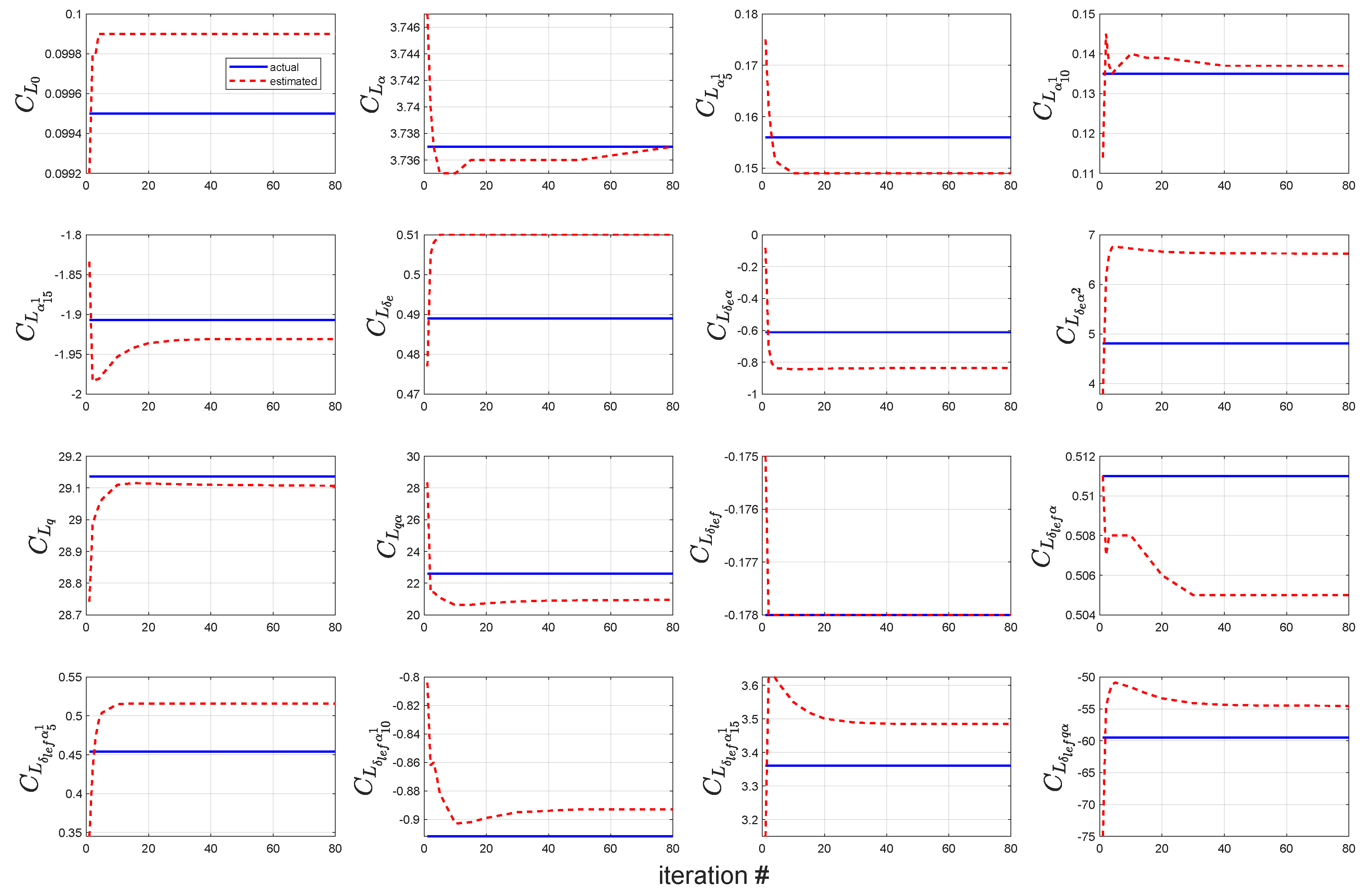
Figure 8 shows the variation in estimated parameters for lift coefficient $C_L$ versus the iteration number. None of the parameters in the proposed model show a variation larger than $50\%$ from the converged solution. As expected, the converged solution is very close to that obtained from the actual thrust value.

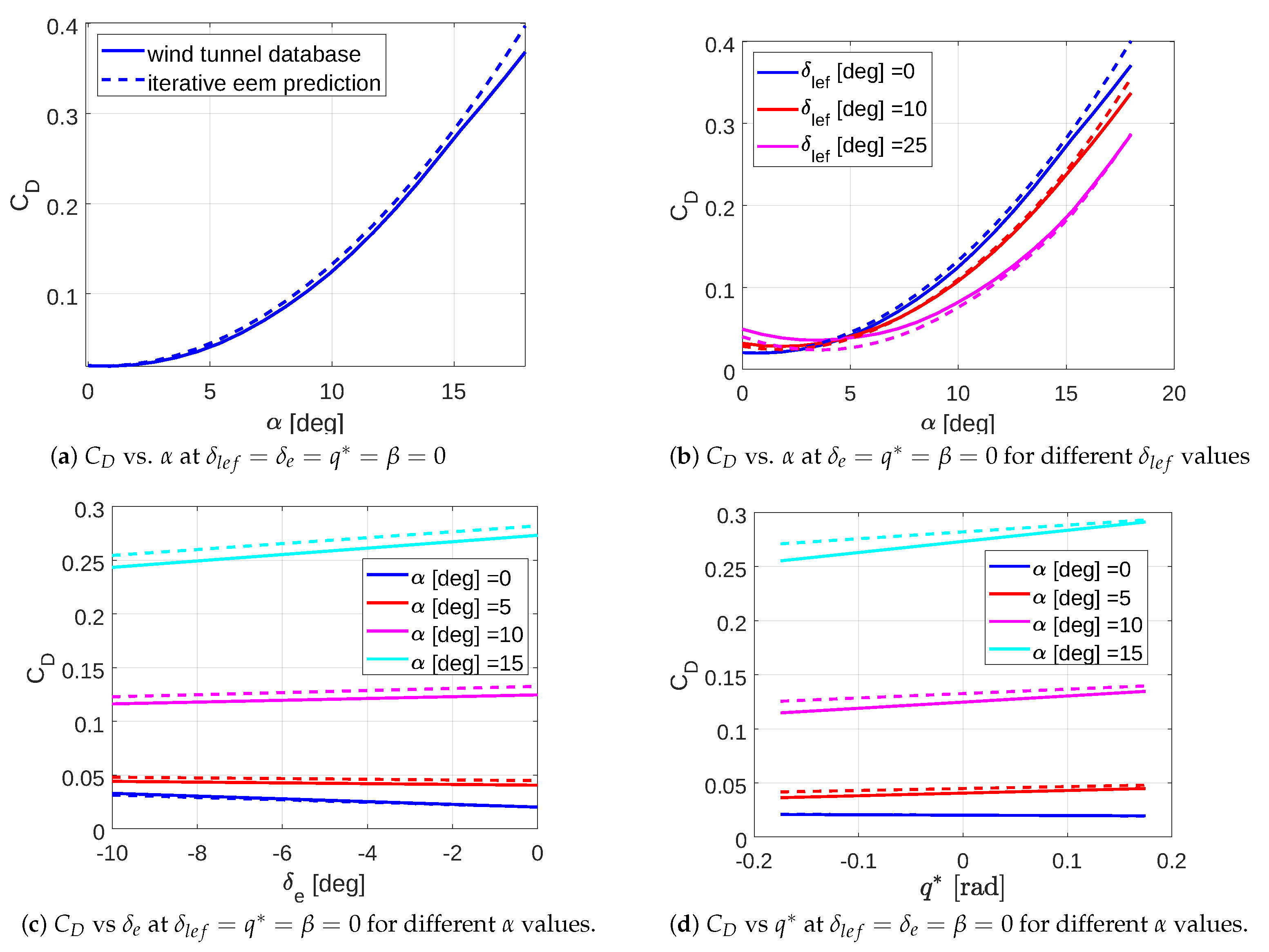
Figure 9 shows a comparison of the estimated parameter values obtained using the IEEM with the true values obtained from the wind tunnel database for coefficient $C_D$. The IEEM initially yielded poor results far from the actual values. However, as the number of iterations increased, the results became closer. The difference in Figure 9b arises from the fact that the leading-edge flap is adjusted according to the angle of attack, where a high angle of attack corresponds to a high leading-edge flap. When the leading-edge flap is zero, the corresponding angle of attack is between $-5^{\circ }$ and $5^{\circ }$. A larger leading-edge flap corresponds to a larger angle of attack (greater than ${10}^{\circ }$).

Figure 10 shows a comparison of the estimated parameter values of coefficient $C_L$ using the IEEM with the actual values obtained from the wind tunnel database. It is easier to estimate the $C_L$ since it has a lower correlation with the engine thrust. A good agreement between estimates and actual values is observed since $C_L$ displays a more linear trend compared to coefficient $C_D$.

5. Conclusions

A methodology was developed based on the iterative equation error method (IEEM) to determine nonlinear aerodynamic and engine thrust models in the absence of engine manufacturer data. The study was based on simulated flight test data from a nonlinear simulation of the F-16 aircraft with realistic noise included. With two different altitudes and six different speed configurations, manoeuvres were carried out for twelve different trim points. Control inputs of the pilot were configured for short-period, phugoid, Dutch roll, and bank-to-bank manoeuvres. Trim data for a set of discrete flight conditions with Mach number ranging from $M=0.2$ to $M=0.6$, altitude from $h=0$ ft to h = 40,000 ft, and flight path angle from $\gamma =-5^{\circ }$ to $\gamma =5^{\circ }$ were collected to develop a generic engine thrust model. Ideally the method should have been tested for a larger range of Mach numbers, but the F-16 model of [21] is limited to a maximum Mach number of 0.6.

The IEEM is a sequential process in which the flight data remain the same and only an estimated variable is modified at each iterative step. The simulation results indicated that the proposed algorithm was effective and could produce a satisfactory estimation accuracy. Furthermore, the parameter separation technique introduced herein can be applied to identify large-scale systems by reducing the number of parameters to be identified, thereby greatly simplifying the system identification process.

The engine model is assumed to be true for the EEM application. Clearly, the more accurate the engine model, the more accurate the drag coefficient estimation. Any error in the engine propulsion model propagates into errors in the measured (constructed) aerodynamic force and moment coefficients and thus leads to changes in the identified model parameters. Therefore, to improve the accuracy of the engine model, the IEEM can be utilized.

References

1. Allerton, D. Principles of Flight Simulation; John Wiley: West Sussex, UK, 2009. [Google Scholar]
2. Kurt, H.B.; Millidere, M.; Gömeç, F.S.; Uğur, O. Multi-fidelity aerodynamic dataset generation of a fighter aircraft. In Proceedings of the AIAA SciTech 2021 Forum, Virtual Event, 11–15 & 19–21 January 2021. Number AIAA 2021-0544. [Google Scholar] [CrossRef]
3. Liu, Q.; Zhang, P.; Xiao, W.; Diao, J.D. Correction methods of aerodynamic force and moment coefficients based on the identification data. In Proceedings of the 2019 Chinese Control Conference (CCC), Guangzhou, China, 27–30 July 2019; pp. 1581–1586. [Google Scholar] [CrossRef]
4. Tyan, M.; Kim, M.; Pham, V.; Choi, C.K.; Nguyen, T.L.; Lee, J.W. Development of advanced aerodynamic data fusion techniques for flight simulation database construction. In Proceedings of the 2018 Modeling and Simulation Technologies Conference, Atlanta, GA, USA, 8–12 January 2018. Number AIAA 2018-3581. [Google Scholar] [CrossRef]
5. Peerlings, B. A Review of Aerodynamic Flow Models, Solution Methods and Solvers and Their Applicability to Aircraft Conceptual Design. Master’s Thesis, Delft University of Technology, Delft, The Netherlands, 2018. [Google Scholar]
6. Yavuztürk, V.; Topbaş, E. Simulation model improvement with aerodynamic parameter estimation techniques. In Proceedings of the AIAA SciTech 2020 Forum, Orlando, FL, USA, 6–10 January 2020. Number AIAA 2020-1645. [Google Scholar] [CrossRef]
7. Haser, S.A. Time domain system identification for an UAV using flight test data. In Proceedings of the Ankara International Aerospace Conference, Ankara, Turkey, 11–13 September 2013. Number 013-065. [Google Scholar]
8. Jategaonkar, R.V. Flight Vehicle System Identification: A Time Domain Methodology; AIAA: Reston, VA, USA, 2015; Volume 245. [Google Scholar] [CrossRef]
9. Morelli, E.A.; Klein, V. Aircraft System Identification: Theory and Practice; AIAA: Reston, VA, USA, 2006. [Google Scholar]
10. Tischler, M.B.; Remple, R.K. Aircraft and Rotorcraft System Identification: Engineering Methods with Flight Test Examples, 2nd ed.; AIAA: Reston, VA, USA, 2012. [Google Scholar]
11. Morelli, E.A.; Grauer, J.A. Practical aspects of frequency-domain approaches for aircraft system identification. J. Aircr. 2020, 57, 268–291. [Google Scholar] [CrossRef]
12. Morelli, E.; Cooper, J. Frequency-domain method for automated simulation updates based on flight data. J. Aircr. 2015, 52, 1995–2008. [Google Scholar] [CrossRef]
13. Thurgood, J.W.; Hunsaker, D.F. Sensitivitiy and estimation of flying-wing aerodynamic, propulsion, and inertial parameters using simulation. In Proceedings of the AIAA SciTech 2021 Forum, Virtual Event, 11–15 & 19–21 January 2021. Number AIAA 2021-1528. [Google Scholar] [CrossRef]
14. Millidere, M.; Cakin, U.; Yigit, T. Generating aerodynamic database from closed loop simulated flight data. In Proceedings of the 8th European Conference for Aeronautics and Space Sciences (EUCASS), Madrid, Spain, 1–4 July 2019. [Google Scholar] [CrossRef]
15. Monstein, R.; Capone, P.; Dettling, M.; Vrdoljak, M. Determination of model structure from flight test with generalized additive models. J. Aircr. 2019, 56, 1281–1742. [Google Scholar] [CrossRef]
16. van Ingen, J.; de Visser, C.C.; Pool, D.M. Stall model identification of a Cessna Citation II from flight test data using orthogonal model structure selection. In Proceedings of the AIAA SciTech 2021 Forum, Virtual Event, 11–15 & 19–21 January 2021. Number AIAA 2021-1725. [Google Scholar] [CrossRef]
17. Paris, A.C.; Bonner, M. Nonlinear model development from flight-test data for F/A-18E Super Hornet. J. Aircr. 2004, 41, 692–702. [Google Scholar] [CrossRef]
18. Grauer, J.A.; Morelli, E.A. A new formulation of the filter-error method for aerodynamic parameter estimation in turbulence. In Proceedings of the AIAA Atmospheric Flight Mechanics Conference, Dallas, TX, USA, 22–26 June 2015. Number AIAA 2015-2704. [Google Scholar] [CrossRef]
19. Millidere, M.; Kurt, H.B.; Ballı, H.; Uğur, O. Kalman based neural network model analysis with resampling methods for longitudinal aerodynamic coefficient estimation. In Proceedings of the AIAA Aviation 2020 Forum, Virtual Event, 15–19 June 2020. Number AIAA 2020-3197. [Google Scholar] [CrossRef]
20. Ghazi, G.; Bosne, M.; Sammartano, Q.; Botez, R.H. Cessna Citation X stall characteristics identification from flight data using neural networks. In Proceedings of the AIAA Atmospheric Flight Mechanics Conference, Grapevine, TX, USA, 9–13 January 2017. Number AIAA 2017-0937. [Google Scholar] [CrossRef]
21. Nguyen, L.T.; Ogburn, M.E.; Gilbert, W.P.; Kibler, K.S.; Brown, P.W.; Deal, P.L. Simulator Study of Stall/Post-Stall Characteristics of a Fighter Airplane with Relaxed Longitudinal Static Stability; NASA Technical Paper 1538; NASA: Washington, DC, USA, 1979.
22. Morelli, E.A. Practical aspects of the equation-error method for aircraft parameter estimation. In Proceedings of the AIAA Atmospheric Flight Mechanics Conference and Exhibit, Keystone, CO, USA, 21–24 August 2006. Number AIAA 2006-6144. [Google Scholar] [CrossRef]
23. Millidere, M.; Karaman, U.; Uslu, S.; Kasnakoglu, C.; Çimen, T. Newton Raphson methods in aircraft trim: A comparative study. In Proceedings of the AIAA Aviation 2020 Forum, Virtual Event, 15–19 June 2020. Number AIAA 2020-3198. [Google Scholar] [CrossRef]
24. Millidere, M.; Karaman, U.; Balli, H.; Çimen, T. Further investigations on Newton-Raphson methods in aircraft trim. In Proceedings of the AIAA Aviation 2021 Forum, Virtual Event, 2–6 August 2021. Number AIAA 2021-0411. [Google Scholar] [CrossRef]
25. Stevens, B.L.; Lewis, F.L.; Johnson, E.N. Aircraft Control and Simulation Dynamics, Controls Design and Autonomous Systems, 3rd ed.; Wiley-Blackwell: Hoboken, NJ, USA, 2015. [Google Scholar]
26. Garza, F.R.; Morelli, E.A. Collection of Nonlinear Aircraft Simulations in MATLAB; NASA Technical Memorandum 212145; NASA: Washington, DC, USA, 2003. [Google Scholar]
27. Yadav, R.; Kapadi, Y.; Pashilkar, A. Aero-thermodynamic model for digital simulation of turbofan engine. In Proceedings of the ASME Turbo Expo 2005: Power for Land, Sea, and Air, Reno, NV, USA, 6–9 June 2005; pp. 63–70. [Google Scholar] [CrossRef]
28. Rory, A.R.; Scott, M.E. Modeling techniques for a computational efficient dynamic turbofan engine model. Int. J. Aerosp. Eng. 2014, 2014, 283479. [Google Scholar] [CrossRef]
29. May, R.D.; Csank, J.; Lavelle, T.M.; Litt, J.S.; Guo, T.H. A high-fidelity simulation of a generic commercial aircraft engine and controller. In Proceedings of the 46th AIAA/ASME/SAE/ASEE Joint Propulsion Conference & Exhibit, Nashville, TN, USA, 25–28 July 2010. Number AIAA 2010-6630. [Google Scholar] [CrossRef]
30. Ghazi, G.; Botez, R.; Messi Achigui, J. Cessna Citation X engine model identification from flight tests. SAE Int. J. Aerosp. 2015, 8, 203–213. [Google Scholar] [CrossRef]
31. Rodriguez, L.F.; Botez, R.M. Generic new modeling technique for turbofan engine thrust. J. Propuls. Power 2013, 29, 1492–1495. [Google Scholar] [CrossRef]
32. Ünsal, D. Estimation of Deterministic and Stochastic IMU Error Parameters. Master’s Thesis, Middle Eastern Technical University, Ankara, Turkiye, 2012. [Google Scholar]
33. Jategaonkar, R.; Thielecke, F. ESTIMA—An integrated software tool for nonlinear parameter estimation. Aerosp. Sci. Technol. 2002, 6, 565–578. [Google Scholar] [CrossRef]
34. Jategaonkar, R.V.; Mönnich, W. Identification of DO-328 aerodynamic database for a Level D flight simulator. In Proceedings of the Modeling and Simulation Technologies Conference, New Orleans, LA, USA, 14–17 August 1997. Number AIAA-97-3729. [Google Scholar] [CrossRef]
35. Simmons, B.M.; Mcclelland, H.G.; Woolsey, C.A. Nonlinear model identification methodology for small, fixed-wing, unmanned aircraft. J. Aircr. 2019, 56, 1056–1067. [Google Scholar] [CrossRef]
36. Jategaonkar, R.; Behr, R.; Gockel, W.; Zorn, C. Data analysis of Phoenix RLV demonstrator flight test. In Proceedings of the AIAA Atmospheric Flight Mechanics Conference and Exhibit, San Francisco, CA, USA, 15–18 August 2005. Number AIAA 2005-6129. [Google Scholar] [CrossRef]
37. Raymer, D. Aircraft Design: A Conceptual Approach, 6th ed.; AIAA: Reston, VA, USA, 2018. [Google Scholar] [CrossRef]
38. Aster, R.C.; Borchers, B.; Thurber, C.H. Parameter Estimation and Inverse Problems; Elsevier: Amsterdam, The Netherlands; Academic Press: Burlington, MA, USA, 2005. [Google Scholar]
39. Jategaonkar, R.; Fischenberg, D.; von Gruenhagen, W. Aerodynamic modeling and system identification from flight data—Recent applications at DLR. J. Aircr. 2004, 41, 681–691. [Google Scholar] [CrossRef]
40. Nocedal, J.; Wright, S.J. Numerical Optimization; Springer: New York, NY, USA, 2006. [Google Scholar] [CrossRef]
41. Grauer, J.A.; Morelli, E.A. Generic global aerodynamic model for aircraft. J. Aircr. 2015, 52, 13–20. [Google Scholar] [CrossRef]
Figure 1. Flight test scope.
Aerospace 11 00008 g001
Figure 2. Flight geometry for the air vehicle.
Aerospace 11 00008 g002
Figure 3. C D 0 values for different gliding flights.
Aerospace 11 00008 g003
Figure 4. Schematics of data preprocessing to compute the aerodynamic force and moment coefficients from flight-measured data (modified from [8]).
Aerospace 11 00008 g004
Figure 5. Comparison of trim-constructed and estimated nondimensional thrust coefficients.
Aerospace 11 00008 g005
Figure 6. Convergence of the cost function during the application of the IEEM.
Aerospace 11 00008 g006
Figure 7. Convergence of parameter estimates for the coefficient C D .
Aerospace 11 00008 g007
Figure 8. Convergence of parameter estimates for the C L coefficient.
Aerospace 11 00008 g008
Figure 9. Comparison of wind tunnel data with the IEEM prediction for C D (40th iteration).
Aerospace 11 00008 g009
Figure 10. Comparison of wind tunnel data with the IEEM prediction for C L (40th iteration).
Aerospace 11 00008 g010