1. Introduction
The Earth is influenced by powerful electromagnetic radiation and high-energy particle radiation released from solar activity. Solar flares are among the most violent explosions in the solar atmosphere and are a major focus of space science research [
1,
2]. Unfortunately, high-energy particles and electromagnetic solid radiation pose a fatal threat to space facilities and deep space exploration safety. High-energy particles can easily break through the surfaces of satellites, causing charging and discharging in satellites and even destroying spaceborne equipment [
3]. A spaceborne solar observation system (SSOS) is an important tool for achieving the real-time tracking, observation, and analysis of the Sun. The SSOS must have high tracking accuracy to achieve real-time and accurate observation data.
The SSOS two-dimensional (2D) turntable presented in this study is a typical mechanical–electrical–control coupled system that generates disturbing forces and torques during the tracking rotation. These forces and torques are caused by manufacturing, assembly and control errors, posing a significant threat to spacecraft pointing and tracking stability, commonly known as the micro-vibration effect [
4,
5,
6,
7]. When these forces are coupled with structural modes, resonance will occur, which may cause catastrophic impacts in many fields, such as earthquakes [
8,
9]. In aerospace, resonance may cause a decrease in satellite pointing accuracy and stability accuracy, further affecting the performance of satellite payloads [
10]. Therefore, the flexible vibrations of the structure’s turntable cannot be ignored and must be considered when designing SSOS systems.
When studying the published literature on the modeling of spaceborne 2D turntables, we discovered that the published literature is primarily focused on control system design [
11,
12], structural design, and structural dynamic modeling [
13,
14,
15,
16,
17]. Wang [
11] used non-magnetic technology to study turntable pointing accuracy and motion control, analyzed the influence of the servo control parameters on the dynamic performance and steady-state error, and tested the turntable angular positioning accuracy. Zou [
15] investigated the micro-vibration characteristics of a spaceborne 2D turntable and conducted a modal and frequency response analysis of the structure, which were later verified by experiments. Yao [
18] established the governing equations of the semi-rigid joints and integrated them into the dynamic equation of the deployable structure. The research mentioned above did not combine a control system model with a structural dynamics model. Moreover, the rigid–flexible coupling effect has not been considered, and the influence of structural high-frequency vibrations on the rigid body motion has been ignored. The challenge is that satellites and their payloads are extremely sensitive to high-frequency micro-vibrations, which can be particularly problematic for deep space exploration. For example, the pixel offset for a high-resolution camera is limited by the frequency [
19]. The higher the observation frequency is, the lower the amplitude of the pixel offset that can be tolerated becomes. Several satellite images are blurred under the influence of micro-vibrations [
20]. Thus, the rigid–flexible coupling cannot be ignored and it should be considered in the model of the SOSS.
To fully consider the impact of the resonance on the SOSS system, this study develops a coupling model integrating mechanical, electrical, and control models. We also investigate the impact of rigid–flexible coupling on this model by establishing a rigid–flexible model (R-F-model) and a rigid model (R-model). This study can provide a reference for the design and optimization of the SOSS system.
The following sections of the paper detail our research on the mechanical–electrical–control coupling model. In
Section 2, we explain how we derived the transfer function model using the Laplace transform. In
Section 3, we present simulations of the R-model and R-F-model acceleration responses under angle tracking mode. We also simulate acceleration responses under different control frequencies to determine the optimal control frequency.
Section 4 outlines the experiments we performed and discusses the results. Finally, in
Section 5, we summarize our findings and conclude this study.
2. Mechanical–Electrical–Control Coupling Model of the Spaceborne Solar Observation System (SSOS)
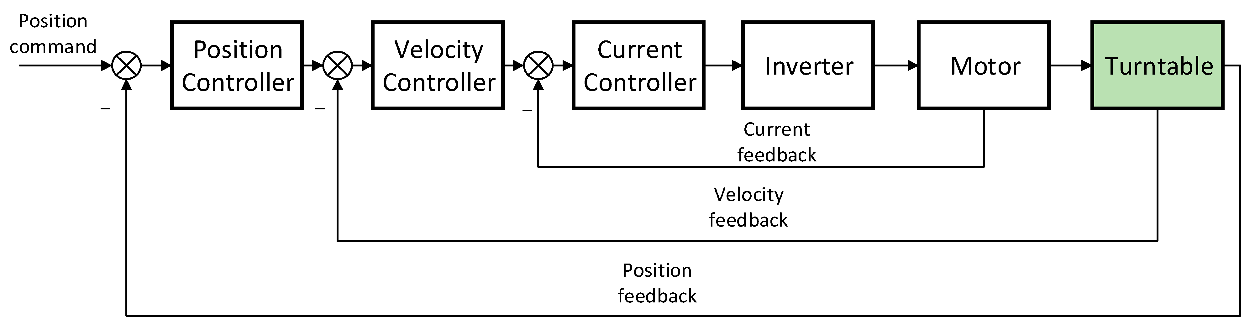
The SSOS is an exciting system that comprises a 2D turntable and an observation payload. The 2D turntable contributes majorly to the dynamic response, and it is composed of various components: a motor, a measurement feedback device, a drive controller, and a power supply.
Figure 1 depicts the schematic diagram of the system, illustrating that the SSOS is a typical mechanical–electrical–control coupled system.
This section establishes the mechanical–electrical–control coupling model, which consists of mechanical, electrical, and control models. We established the R-F-model and R-model to investigate the influence of the structural flexibility on the model’s accuracy.
2.1. Mechanical Model
Based on Newton’s Law, the SSOS mechanical dynamics model based on its rotational degrees of freedom is expressed as follows [
21]:
where
is the rotation angle,
is the moment of inertia of the motor rotor,
is the damping torque coefficient,
is the motor torque, and
is the inertial torque. Due to the approximately unconstrained rotation of the rotor, the stiffness part is ignored.
The inertial motion of the moving components generates an inertial torque. Therefore, when the structure is assumed to be a rigid body, the angular acceleration of the rotating component generates an inertial torque. The turntable’s motion includes its rigid body motion and elastic vibrations when the structure is assumed to be an elastic body. Therefore, the rigid–flexible coupling characteristics should be considered. The inertial torques of the R-model and R-F-model are established to analyze the impact of the structural flexibility, as follows.
- (a)
Inertial torque of R-model
Assumptions:
For the R-model, the rotating component is assumed to be a rigid body.
The inertial torque of the rigid body can be expressed as:
where
is the moment of inertia of the SSOS rotating component.
- (b)
Inertial torque of R-F-model
Assumptions:
For the R-F-model, the rotating component is assumed to be a flexible body, so the flexible vibration and the rotational motion of the rotating component are coupled.
The rigid–flexible coupled dynamics equations are expressed as follows:
where
is the modal coordinate vector,
is the modal participation factor matrix,
is the modal frequency matrix,
is the
n-order identity matrix,
n is the modal order, and
is the modal damping ratio. Finite element analysis can be used to determine the modal participation factors and modal frequencies, and engineering experience suggests that the modal damping ratio is between 0.03 and 0.05 [
22]. The inertial torque can be obtained by solving Equation (3).
2.2. Electrical Model
This section presents the motor torque, and the voltage equation of the motor circuit is expressed as follows:
where
is the circuit resistance,
is the current,
is the inductor, and
is the voltage. Moreover,
is the counter electromotive force generated by the rotation of the motor, and
is the counter electromotive force coefficient. The motor torque is expressed as follows:
where
is the motor torque coefficient. The motor voltage and torque equation derivations are presented in
Appendix A [
23].
2.3. Servo Control Model
The SSOS adopts a three-loop control system, as shown in
Figure 1. The speed loop and the current loop are proportional–integral (PI) controllers, with proportional control of the position loop. The control instruction of the position loop is expressed as follows:
where
is the angle error,
is the angle instruction,
is the feedback angle, and
is the parameter of the position loop controller.
The speed loop control instruction is expressed as follows:
where
is the angular velocity error,
is the angular velocity feedback coefficient,
is the mechanical angular velocity of the motor,
, and
and
are the parameters of the speed loop controller.
The control instruction of the current loop is expressed as follows:
where
is the current instruction,
is the current feedback coefficient, and
and
are the parameters of the current loop controller.
The inverter is simplified as an inertial system, and the relationship between the output voltage and the input voltage is as follows:
where
and
are the inverter gain and the time constant, respectively.
2.4. State-Space Equation of the System
This section establishes the state-space equation of the system based on the discussions in
Section 2.1,
Section 2.2 and
Section 2.3. The mechanical–electrical–control coupling model is obtained based on Equations (1)–(9):
where
The state-space Equation (10) is expressed as follows:
- (a)
State-space equation of the R-model
We define
and combine Equations (2) and (12). The state-space equation of the R-model can be expressed as follows:
- (b)
State-space equation of the R-F-model
We define
,
,
,
, and
, and combine Equations (3) and (12). Then, the state-space equation of the R-F-model can be expressed as follows:
Equation (13) lacks some critical parameters, such as the modal frequency, damping, and participation factor, which are essential in actual structures. In contrast, these parameters significantly contribute to the description of the rigid–flexible coupling characteristics in the state-space equation of the model, as shown in Equation (14). Based on the above information, the importance of the R-F-model is indicated by comparing Equations (13) and (14).
2.5. Transfer Function and Simulink Model of SSOS
It is challenging to quickly determine the impact of the relevant factors on the SSOS performance using the state-space model obtained in
Section 2.4. Therefore, we established a Simulink model to simplify the process, which required the use of transfer functions obtained by performing the Laplace transform of each module in
Section 2.1,
Section 2.2 and
Section 2.3. The mechanical model’s transfer function is expressed as follows:
The motor transfer function is expressed as follows:
The position controller transfer function is expressed as follows:
The speed controller transfer function is expressed as follows:
The current controller transfer function is expressed as follows:
The transfer function of the inverter is expressed as follows:
The transfer function of the inertial torque of the R-model is expressed as follows:
The transfer function of the inertial torque of the model is expressed as follows:
Note that
, where
is the rigid torque, and
is the flexible torque. Then, Equation (22) is divided into two parts, where the transfer function of the rigid torque is expressed as follows:
The transfer function of the flexible torque is expressed as follows:
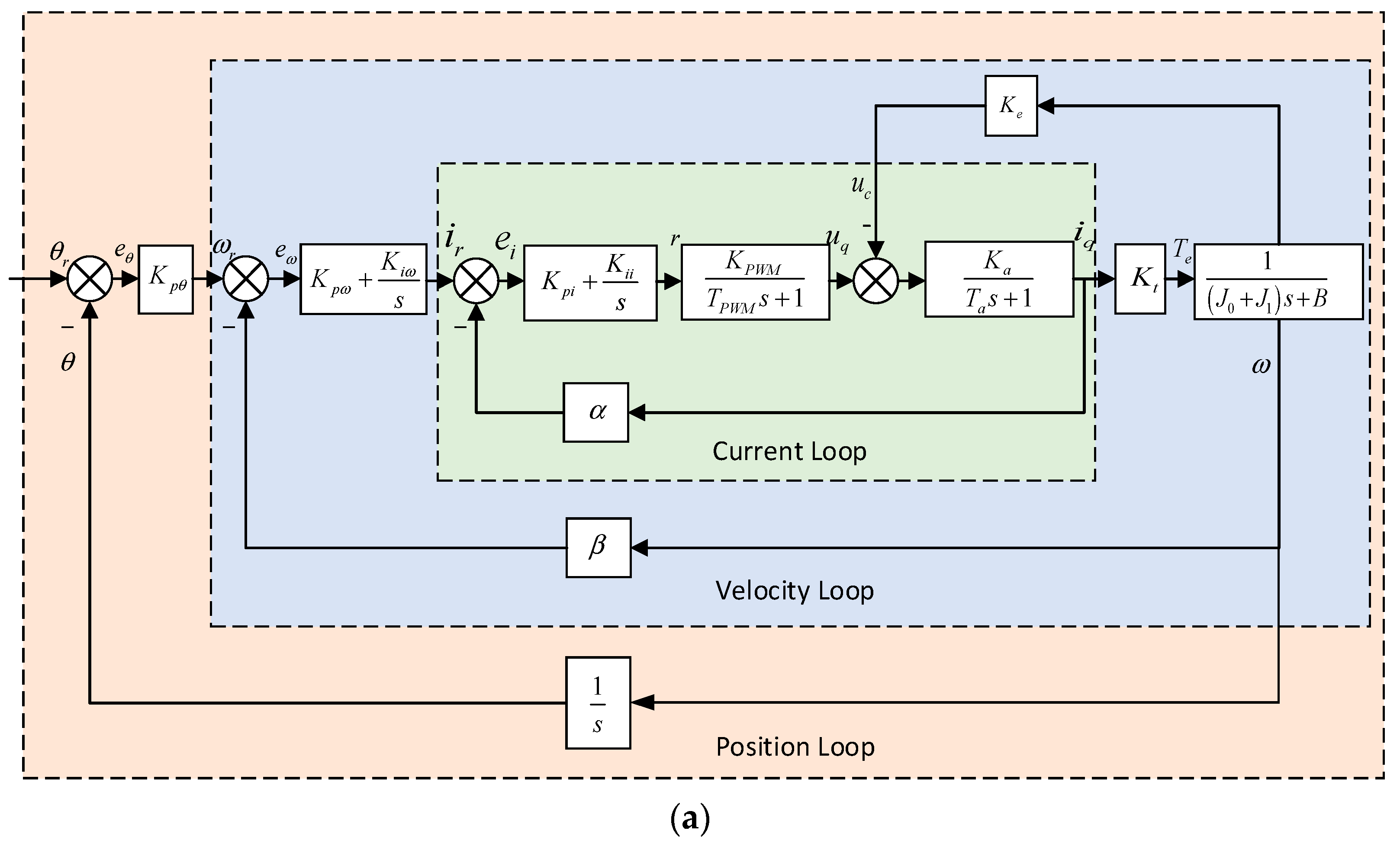
As illustrated in
Figure 2, we combined the transfer functions of the modules mentioned above to create two schematic diagrams, where (a) shows the schematic diagram of the R-model, and (b) shows the schematic diagram of the R-F-model.
3. Simulations of SSOS
We established a Simulink model to analyze the SSOS dynamic characteristics based on the schematic diagram in
Section 2. The natural frequency of the turntable may couple with the excitation frequency, causing resonance. Therefore, it is necessary to calculate the natural frequency of the turntable structure. These external excitations may arise from the control frequency of the motor, motor noise, and nonlinear factors. Thus, we built a finite element method (FEM) model of the 2D turntable to investigate the effect of the rigid–flexible coupling characteristics. Moreover, we obtained the modal frequencies and participation factors [
8,
9] of the SSOS through FEM analysis and additional calculations.
3.1. Finite Element Method (FEM) Modeling and Simulations of Two-Dimensional (2D) Turntable
3.1.1. FEM Model and Modal Analysis
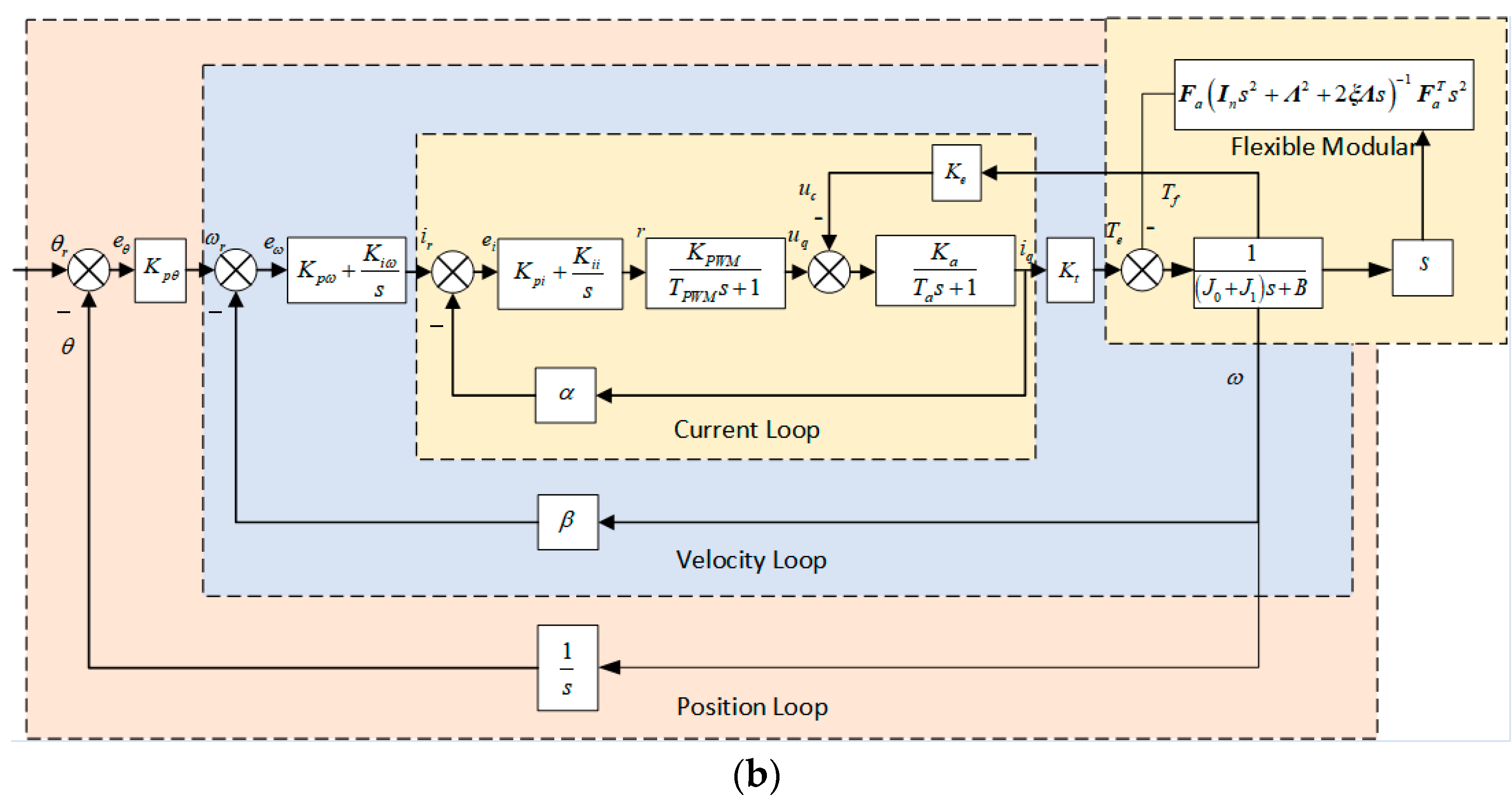
The 2D turntable has dimensions of 463 mm × 336 mm × 550 mm and weighs 23 kg. The 2D turntable FEM model was established. A mesh convergence study was conducted and mesh size 10 was adopted. The first 10 modes were calculated through modal analysis.
Figure 3 depicts the first three modal deformation cloud diagrams, and
Table 1 presents the first 10 modal frequencies. The natural frequencies of the 2D turntable are all higher than 100 Hz, and 0.03 is the modal damping ratio.
3.1.2. Modal Participation Factors
Since the turntable only moves via rotation, the rotational modal participation factor is expressed as follows:
where
represents the mass of node
i,
N is the total number of nodes,
is the vector of node
i relative to the reference point, and
represents the modal vector matrix of node
i, where
n is the modal truncation order. We calculated the generalized modal effective mass and its proportional factor relative to the moment of inertia to determine the modal truncation order. The modal effective mass of the first
n modes is expressed as follows:
The proportional factor of the first
n modal effective masses is expressed as follows:
We computed the first 10 modes’ participation factors (unit:
) based on Equation (25), and the results are presented in
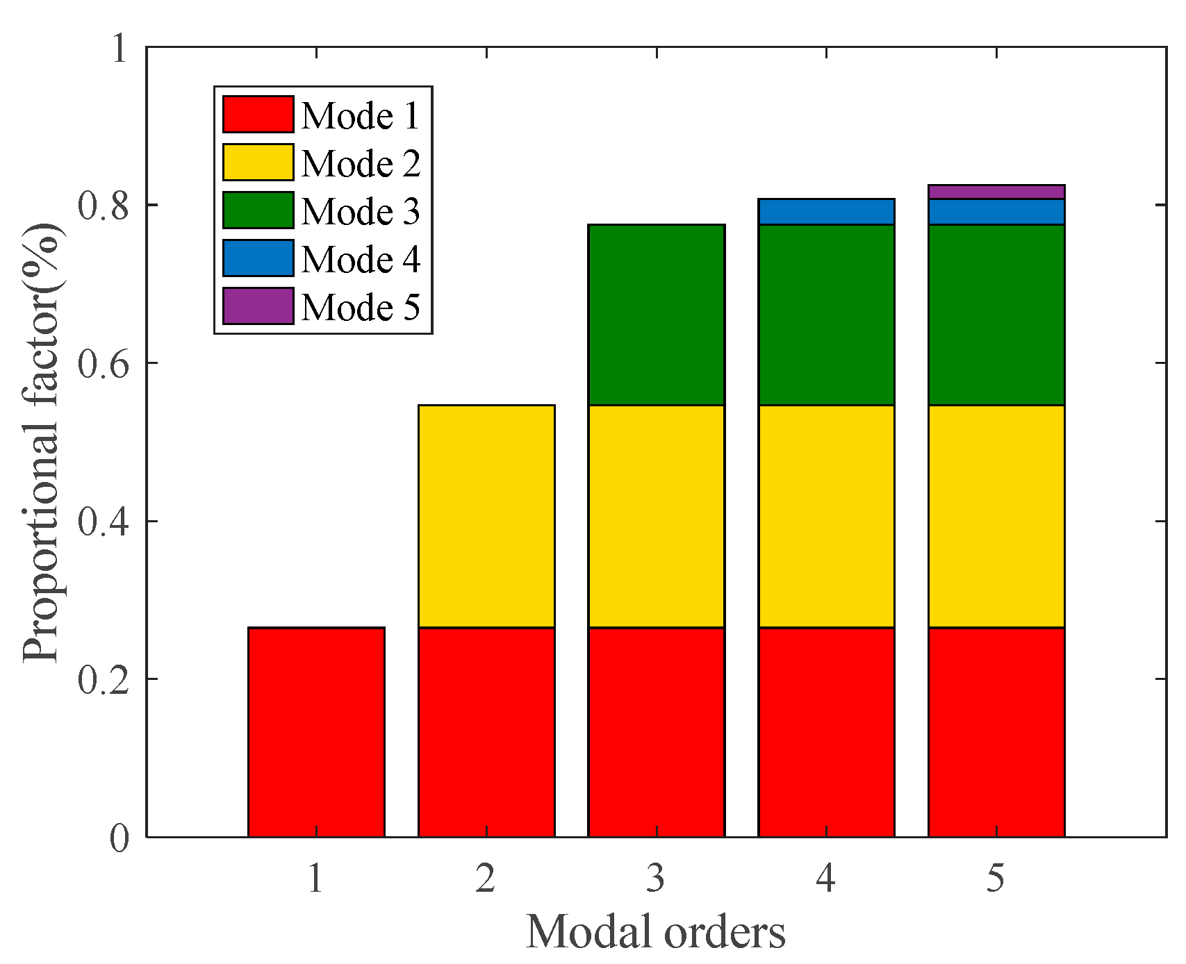
Table 1. Moreover, we calculated the first five modes’ proportional factors, based on Equations (26) and (27), as shown in
Figure 4, where each column represents the proportional factor of the first
n modes. The larger the proportional factor is, the closer it is to the actual vibration.
Figure 4 shows that the modal proportional factors of the first three modes reached 80%. As the modal order increased, the proportional factor increased slightly. As a result, the modal truncation order was selected as 3 in the simulation, considering both the accuracy and the calculation complexity.
3.2. Simulation of SSOS
In this section, we established a Simulink model, which was used to perform simulations with the R-model and R-F-model to analyze the impact of rigid–flexible coupling on the turntable’s rotation angles and acceleration responses. Thereafter, we performed simulations with the R-model and R-F-model for different control frequencies to obtain the optimal value of the control frequency. The control frequency represents the number of instruction signals per second. In order to avoid resonance caused by coupling between the control frequency and the natural frequency of the turntable, we selected control frequencies that are lower than 1/10 of the turntable’s natural frequency.
3.2.1. Simulink Model
The Simulink simulation model of the R-F-model was built based on the schematic diagram in
Figure 2. Some parameters of the turntable’s pitch axis are presented in
Table 2, and the flexible module was disabled when R-model simulations were conducted.
3.2.2. Acceleration Response Simulation under Angle Tracking Mode
The SSOS mainly operates in an angle tracking mode, and its axis always points to the Sun. The solar altitude from 6:00 to 6:01 on March 24 was selected based on the simulation input data, and the control frequency was 1 Hz.
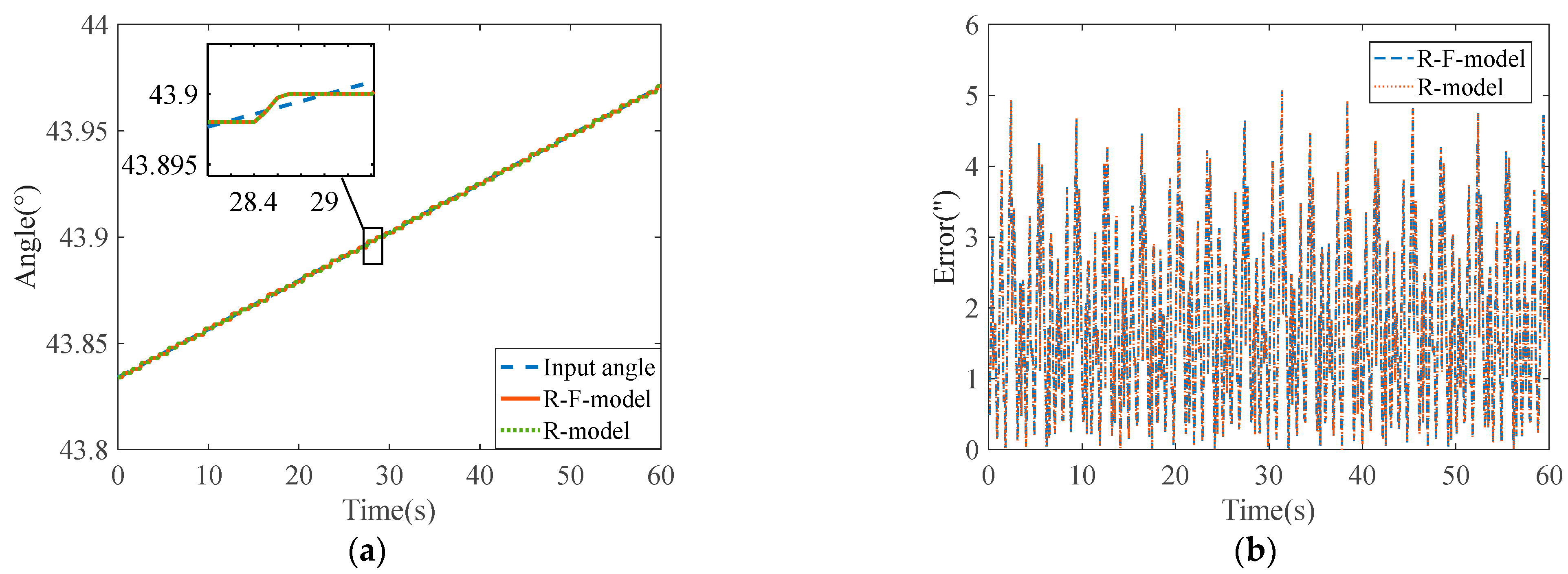
Figure 5a shows the tracking angle of the R-F-model and R-model, where the red solid line is the curve of the R-F-model. The green dotted line is the curve of the R-model, and the blue dashed line is the input angle.
Figure 5b depicts the R-F-model and R-model angle tracking errors.
Figure 5 shows that the angles of the R-F-model and R-model are similar, and the angle tracking errors are less than 5”. Based on this figure, theoretically, the turntable’s structural flexibility with high natural frequencies has little influence on the angle tracking.
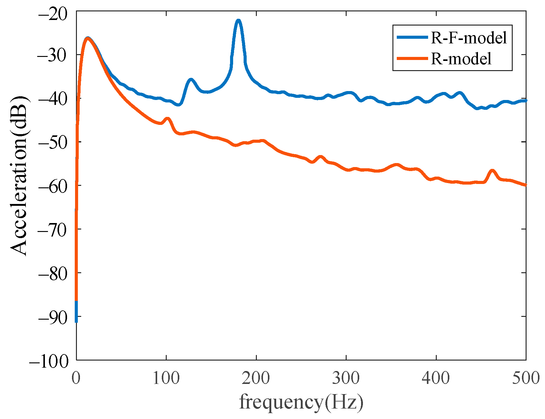
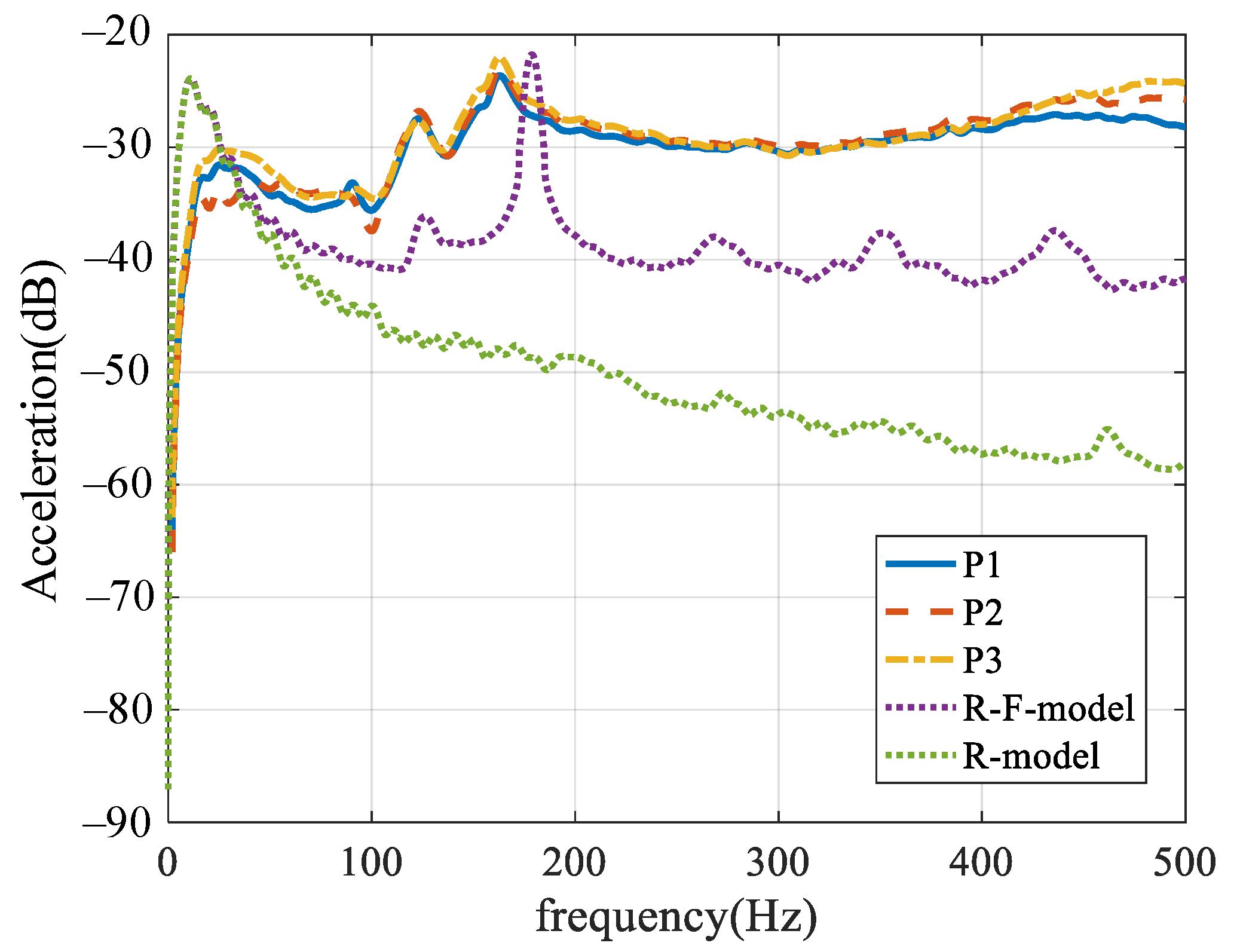
Figure 6 shows the acceleration spectral curves, indicating that the acceleration spectra of the R-F-model generated peak responses in high frequencies caused by structural flexibility compared with the R-model. Eventually, the extra responses caused by the structural flexibility would affect the SSOS. The simulation results indicate that the rigid–flexible coupling characteristic has little influence on the angle tracking of the simulation model. However, this rigid–flexible coupling affects the high-frequency distribution of the acceleration spectrum. This mechanism is essential for a spaceborne SSOS, as micro-vibrations at a high frequency may negatively affect the satellites’ stable precision and the image definition of optical cameras. Therefore, this issue requires attention, which is verified in
Section 4. Overall, the proposed coupling model can describe the difference between the R-model and the R-F-model.
3.2.3. Acceleration Response Simulations under Various Control Frequencies
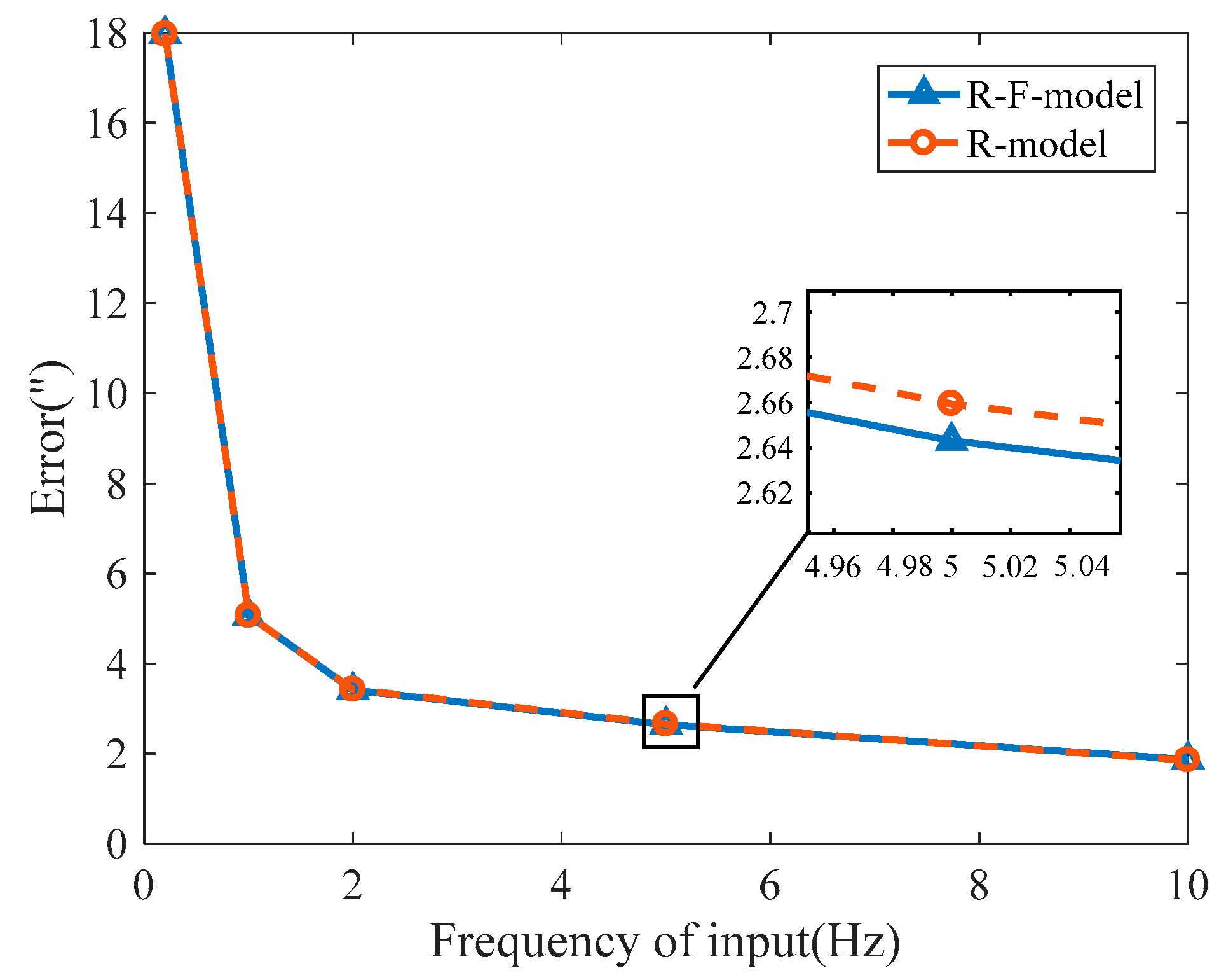
We input the angle commands at different frequencies to conduct dynamic simulations, selecting the solar altitude from 6:00 to 6:01 on March 24 as the simulation input data, where the control frequencies were 0.2, 1, 2, 5, and 10 Hz. The maximum angle tracking error curves under different control frequencies were obtained through simulations, as shown in
Figure 7, where the solid blue line is the R-F-model’s simulation result, and the dashed red line is the R-model’s simulation result. These results indicate that the angle tracking error decreases as the control frequency increases. The maximum angle tracking error is less than 5″, and it satisfies the angle tracking requirement when the control frequency is higher than 1 Hz.
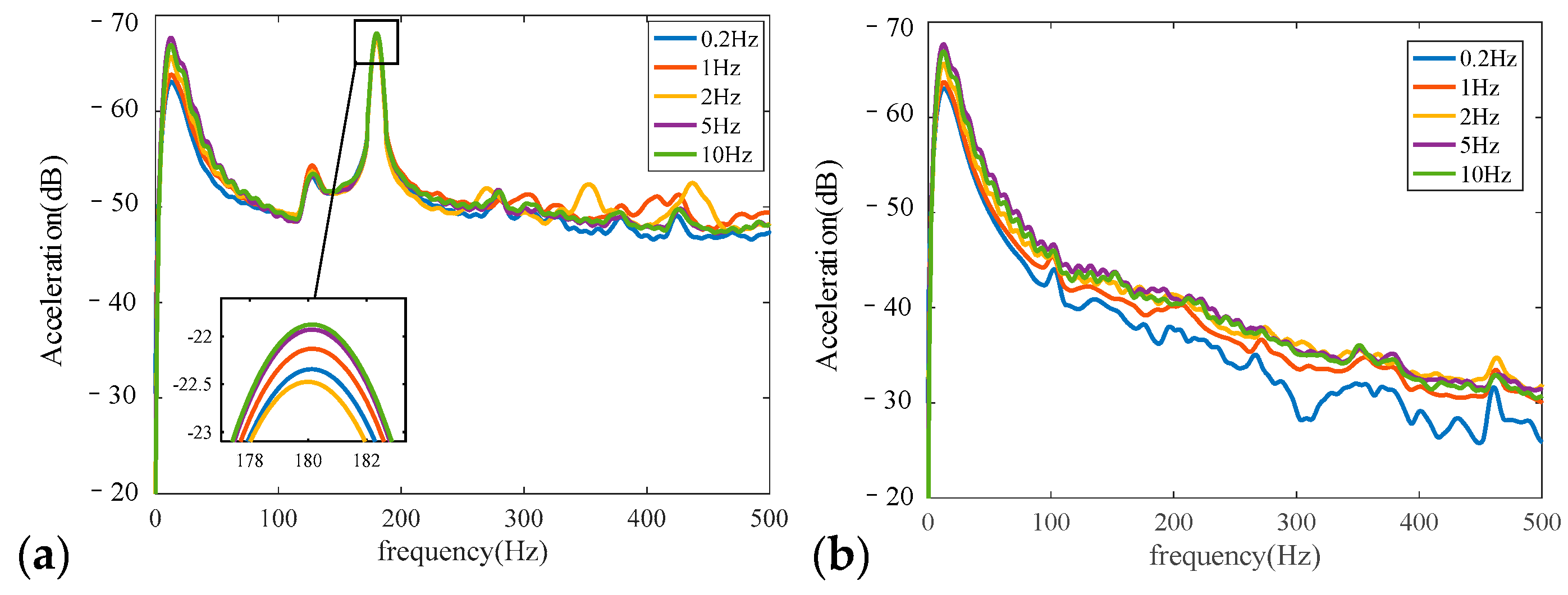
Figure 8 shows the acceleration spectral curves under different control frequencies, where (a) shows the acceleration spectral curve of the R-F-model, and (b) shows the acceleration spectral curve of the R-model. The third modal frequency of the turntable is 180.2 Hz (
Table 1), which amplifies the vibration of the turntable, resulting in a peak acceleration at about 180 Hz in
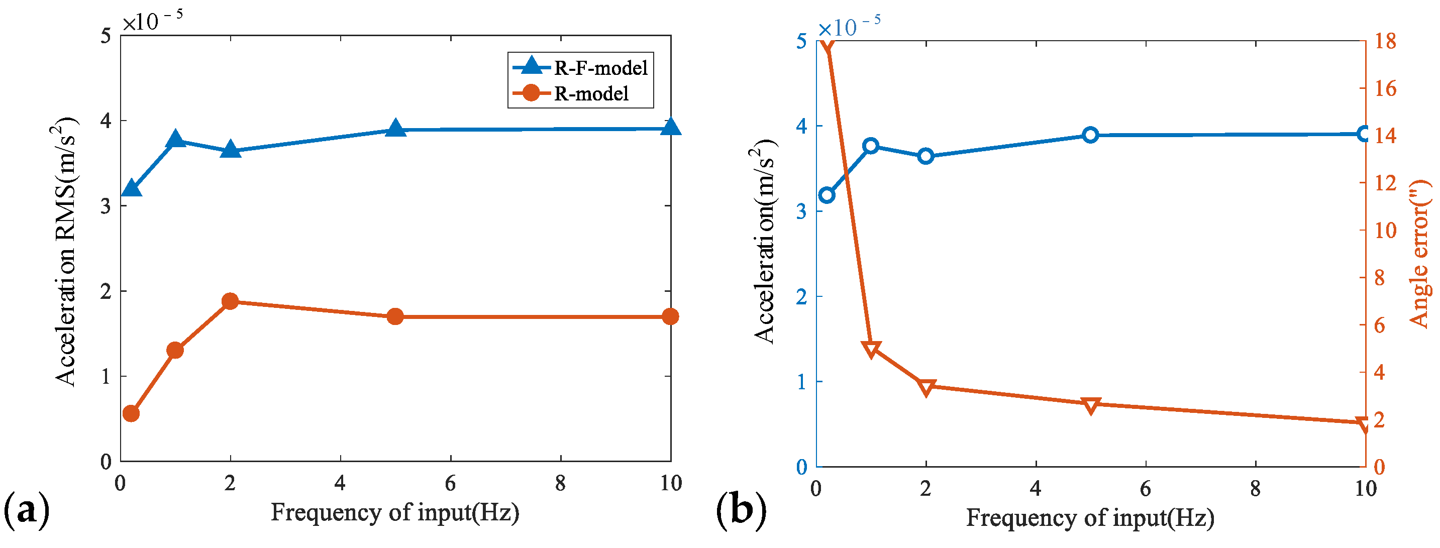
Figure 8. Moreover, the acceleration peak value increases as the control frequency increases. We calculated the acceleration response’s root mean square (RMS) values under different control frequencies, as shown in
Figure 9a. Interestingly, the RMS of the acceleration response of the R-F-model is two times larger than that of the R-model. The RMS of the acceleration response shows an upward trend as the control frequency increases. To obtain the optimal control frequency of the SSOS, the acceleration RMS and maximum angle tracking error were plotted, as shown in
Figure 9b. The acceleration RMS and the angle tracking error shows opposite trends. When the input frequency was 2 Hz, the angle tracking error is less than 5″, lower than the precision SSOS requirement. The angle tracking error tends to be convergent, and the acceleration RMS is relatively small at the same time. As a result, 2 Hz was selected as the control frequency when developing the SSOS.
5. Conclusions
The purpose of this study is to investigate how the elastic characteristics and control frequency impact micro-vibration acceleration responses in a high-precision SSOS. To achieve this goal, we developed the R-F-model and R-model of the SSOS, and analyzed the effect of rigid–flexible coupling by establishing the state-space model. We then built a Simulink model using the Laplace transform to derive a transfer function model. By simulating the R-F and R-model acceleration responses under the angle tracking mode, we observed differences when flexible features were considered. Specifically, the RMS of the model’s acceleration response was found to be two times larger than that of the R-model. We also conducted simulations with various control frequencies to determine the optimal value. Finally, we conducted experiments and validated the theoretical model and simulation results using measured data under different control frequencies (1, 2, 5, and 10 Hz). Our findings suggest that the flexibility of the structure affects the high-frequency distribution of the acceleration spectra and poses threats to the high tracking accuracy. This study highlights the significance of elastic structures in dynamic response and provides a valuable reference for the design and micro-vibrations of spacecraft structure systems.


