Robust Trajectory Prediction Using Random Forest Methodology Application to UAS-S4 Ehécatl

Abstract

Accurate aircraft trajectory prediction is fundamental for enhancing air traffic control systems, ensuring a safe and efficient aviation transportation environment. This research presents a detailed study on the efficacy of the Random Forest (RF) methodology for predicting aircraft trajectories. The study compares the RF approach with two established data-driven models, specifically Long Short-Term Memory (LSTM) and Logistic Regression (LR). The investigation utilizes a significant dataset comprising aircraft trajectory time history data, obtained from a UAS-S4 simulator. Experimental results indicate that within a short-term prediction horizon, the RF methodology surpasses both LSTM and LR in trajectory prediction accuracy and also its robustness to overfitting. The research further fine-tunes the performance of the RF methodology by optimizing various hyperparameters, including the number of estimators, features, depth, split, and leaf. Consequently, these results underscore the viability of the RF methodology as a proven alternative to LSTM and LR models for short-term aircraft trajectory prediction.

1. Introduction

The horizon of aviation is rapidly expanding, with Unmanned Aerial System (UAS) development. As these systems perform increasingly complex missions and operate in different environments [1], their need for precise trajectory prediction is undeniably crucial [2]. Aircraft trajectory prediction (ATP) involves forecasting an aircraft’s future position and motion based on its current and previous positions, as well as on environmental and operational factors [3]. This is a crucial task for Air Traffic Management (ATM) [4,5], as it can ensure safety requirements [6,7,8] and the efficiency of flights [9] by allowing controllers [10,11] to detect potential conflicts [12] and to adjust flight paths accordingly [13,14].

Aircraft trajectory prediction can be formulated as a time-series problem [15]. In a time-series analysis, data points are collected or recorded at successive points in time, with the goal often being to predict future values based on historical data. In the ATM context, the historical data refer to previous positions, velocities, accelerations, and other relevant aircraft parameter variations over time [16].

A variety of classical methodologies have been successfully employed for time-series ATP analysis in ATM development [17,18]. State-space models, which utilize the Kalman filter, have been explored for trajectory prediction in aviation [19]. By modeling the aircraft dynamics and observation processes, the Kalman filter can predict future aircraft positions even in the presence of measurement noises. Although an adaptive state-space model could accurately perform the ATP task using Automatic Dependent Surveillance–Broadcast (ADS-B) data [19], its performance was affected by computational complexity [20]. In other words, in scenarios where predictions are required for multiple aircraft simultaneously, computational cost becomes the limiting factor. The Autoregressive Integrated Moving Average (ARIMA) model is a classic statistical method for time-series forecasting [21]. Despite this, the ARIMA was used for trajectory simulation and prediction [22] with minimal data pre-processing, making it suitable for short-term trajectory predictions.

Memory-based modern methodologies were developed for improving long-term predictions and processing time. Recurrent neural networks (RNNs) can model sequences and have been explored for predicting aircraft trajectories [23]. In reference [24], for instance, the authors trained a neural network to predict an aircraft’s future path by modeling trajectory data as a time series. RNN could perform fast 4D ATP for the UAS-S4, which then was developed into Long Short-Term Memory (LSTM) [25]. LSTM networks are designed as a specific type of RNN architecture, with the aim of remembering patterns over long time sequences. They are particularly suitable for applications such as the ATP, where the flight history of an aircraft can influence its future path [26]. Despite their speed and accuracy in ATP, they were found to be vulnerable when faced with uncertainties such as noise in data (due to signal blockage and interference), missing values (due to miscommunications), and misleading values (due to adversarial attacks) [27]. As a result, ‘ensemble’ methods have been proposed for robust predictions.

When it comes to nonlinearity interactions, feature scaling, handling missing values, ease of interpretation and implementation, and sensitivity to hyperparameter tuning, the RF algorithms outperform data-driven algorithms such as the LSTM, RNN, CNN, and SVM methods. Random Forests are inherently effective at modeling non-linear relationships and complex interactions among features. Trajectory prediction often involves complex interactions between various factors such as speed, acceleration, direction, and environmental factors, which Random Forests can capture effectively. Unlike algorithms such as SVMs and neural networks (CNN, RNN, and LSTM), Random Forests do not require input features to be scaled or normalized. This can be particularly advantageous in trajectory prediction, where features might have different units and scales. Random Forests can handle missing data in the input features better than algorithms such as SVMs and traditional neural networks. This is crucial in real-world trajectory prediction scenarios where sensor data might be incomplete or partially missing. Random Forests, being a collection of decision trees, are relatively easier to interpret and understand than complex models such as LSTM, RNN, and CNN. This can be important for trajectory prediction in safety-critical applications where understanding the decision-making process is crucial. While models such as SVMs and neural networks can be quite sensitive to hyperparameter settings, Random Forests are often easier to tune, or even perform reasonably well with default settings.

Moreover, due to their ensemble nature, where multiple decision trees vote for the final prediction, Random Forests are less prone to overfitting compared to models such as SVMs, especially in scenarios with a large number of features. Given the uncertainties and complexities of aircraft flight dynamics, and environmental factors such as weather, ‘ensemble’ methods that combine predictions from multiple models have also been investigated to increase prediction robustness [28]. When considering fault tolerance, ‘ensemble’ learning methodologies have exhibited exceptional performance [29]. These methods combine predictions from various models, enhancing both accuracy and robustness. Ensemble techniques aggregate the outputs of individual models, thus reducing the effect of errors. The Random Forest (RF) method is an ‘ensemble’ learning algorithm that builds a collection of decision trees [30]. By combining the predictions of these trees through majority voting and averaging, the RF model becomes more resilient to faults [31], noise [32], and adversarial attacks [33].

The contribution of this study can be highlighted as the following:

i.

Initially, the trajectory prediction of the UAS-S4 was transformed into a problem of time-series regression.

ii.

Subsequently, an efficient Random Forest (RF) architecture was developed and tailored to fit the trajectory patterns of the UAS-S4.

iii.

Lastly, a method was designed for optimizing the hyperparameters and feature functions of the Random Forest.

Section 2 articulates the problem related to ATP. The RF methodology and its optimization for performing the ATP task are thoroughly explained in Section 3. Following this, Section 4 provides the examination and comparison of the RF model results with the LR and LSTM models. Finally, Section 5 concludes by summarizing the accomplishments and contributions made through this present study.

2. Problem Statement

It is assumed that a flight area consists of multiple aircraft flying within their designated air corridors. Given the GPS data of the aircraft at a specific time Tn, including latitude, longitude, altitude, heading, speed, and time, a model can be developed to predict the data for the subsequent i intervals [27]. This sequential trajectory prediction within an air corridor is shown in Figure 1.

When formulating ATP as a time-series problem, the goal is to use past flight data to predict future positions and paths of aircraft. To achieve this aim, the following step-by-step procedure should be passed to design an efficient ATP model. With this aim, there exist three main objectives that need to be satisfied. The first is the conversion of the UAS-S4 trajectory prediction into a time-series regression problem. The second is developing an efficient RF architecture compatible with the UAS-S4 trajectory patterns. The third is the design of a procedure for the optimization of the RF hyperparameters and features function.

In designing a reliable prediction system, the initial step is the collection of historical data related to aircraft trajectories [34]. This step involves gathering data points such as positions, velocities, and other relevant parameters of an aircraft, recorded over specific time intervals. Collecting a substantial amount of these pertinent data is important for developing a robust predictive model, as it allows for the analysis and understanding of previous aircraft movement patterns and behaviors.

After collecting the raw data, the next imperative step is feature engineering [35]. This process involves extracting and formulating essential features or factors from the raw data that significantly influence trajectory predictions. Features corresponding to sensor data were taken into account. We considered the following sensor data for training the RF model.

i.

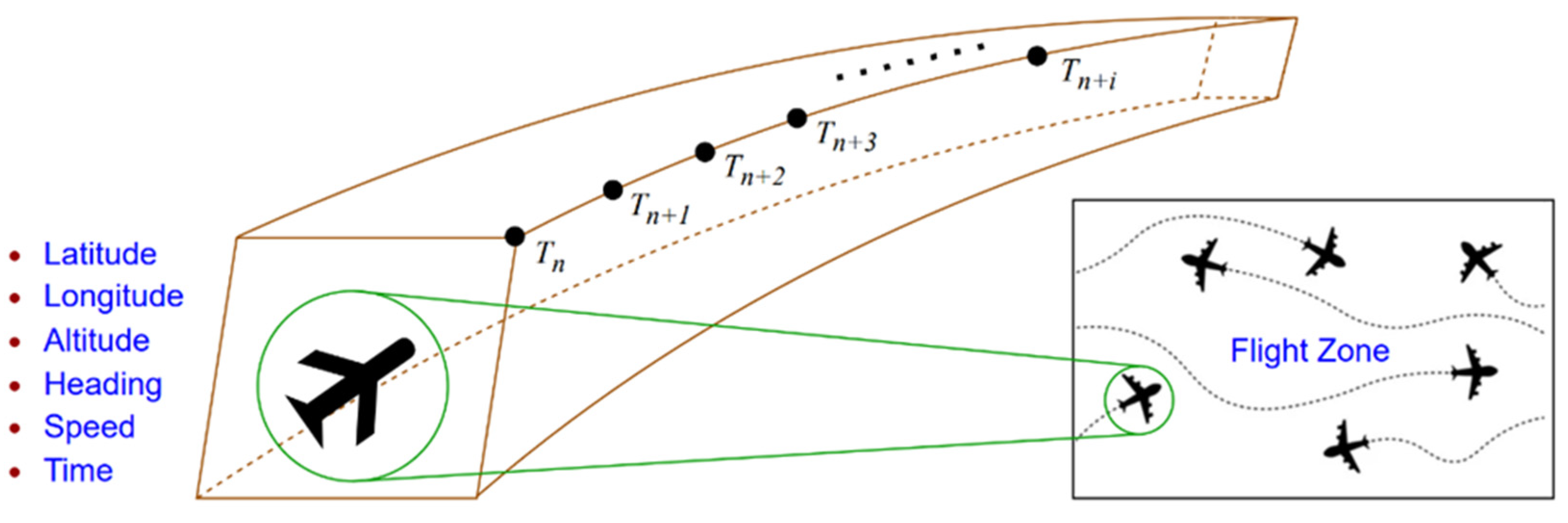
Location coordinates, for which the GPS provided latitude, longitude, and altitude data.

ii.

Speed, derived from changes in position over time.

iii.

Heading, obtained from compass data indicating the direction in which the UAS-S4s were moving.

iv.

Time stamps, for which the time intervals between data points were considered for capturing the dynamics of movement.

v.

Derived features, including distance traveled over a period, average speed, and rate of turning, were engineered from raw sensor data.

By identifying and engineering these crucial features, the raw data were transformed into a more useful and insightful format that enhances the effectiveness of the predictive models.

For the engineered features, various time-series models were then applied to the data [36]. Time-series models are suitable for this task as they are designed to understand and predict sequential data effectively. These models range from traditional ones, such as Autoregressive Integrated Moving Average (ARIMA), to advanced, data-driven structures, such as the LSTM and RFs. Each of these models brings unique strengths to their processing and predicting based on sequential data, providing different options to choose from based on the specific requirements and nature of the data.

Aircraft trajectory is not solely determined by its previous positions. There are external factors or exogenous variables [37] that significantly influence the aircraft path. These factors include meteorological conditions, airspace constraints, and specific performance metrics of the aircraft itself. Due to the impact of these external elements, they are incorporated into the prediction models as additional inputs, thereby improving the accuracy and reliability of the trajectory prediction model.

Model validation is a crucial step in analyzing the effectiveness and reliability of the developed prediction model. It is essential to ensure that the model is not simply over-fitted to the training data [38], which would limit its ability to generalize to unseen data [39]. During this phase, the model is trained on a subset of the collected data and subsequently tested and validated on a separate set of unseen data to objectively evaluate its predictive performance and accuracy.

Once the model is validated and deemed reliable, it is then deployed for predicting future trajectories. Leveraging both current and past trajectory data, the model can actively forecast future paths that aircraft are more likely to take. Such a capability is indispensable for ATM and planning purposes.

The proposed time-series analysis provides a systematic method for anticipating an aircraft’s future trajectory based on its historical path. However, the intricacy of real-world flight dynamics means that this approach may need to be refined for optimal accuracy. In other words, as flight dynamics are subjected to continuous changes due to various factors, the time-series prediction model would need to be regularly updated and refined [40]. As new data on aircraft trajectories become available, incorporating these data to update the model is crucial. This iterative refinement process ensures that the model remains accurate and effective in predicting aircraft trajectories over time by adapting it to the aircraft flight dynamics.

3. Methodology

The RF model is an ‘ensemble’ machine learning method that combines multiple decision trees to perform predictions. In this technique, each decision tree undergoes training using a random subset (fold) of the available data and considers only a random subset for each branch. During the trajectory prediction phase, the RF output is determined by aggregating the predictions from all individual decision trees. In our time-series regression scenario, the RF model is supposed to calculate the average of these predictions. This process involves training the model with a trajectory dataset and using it to predict future trajectories, as follows [41]:

• Data Collection: The UASs’ time history flight trajectory data were generated and collected using the UAS-S4 simulator. These data included latitude, longitude, altitude, heading, speed, and time.
• Data Preprocessing: Firstly, data cleaning incorporated handling missing values, outliers, and noise. Secondly, features were engineered [42], and new features that may be relevant to the memory for the ATP were created. For instance, historical trajectory points can be used to create features including ‘previous_latitude’, ‘previous_longitude’, and ‘previous_altitude’.
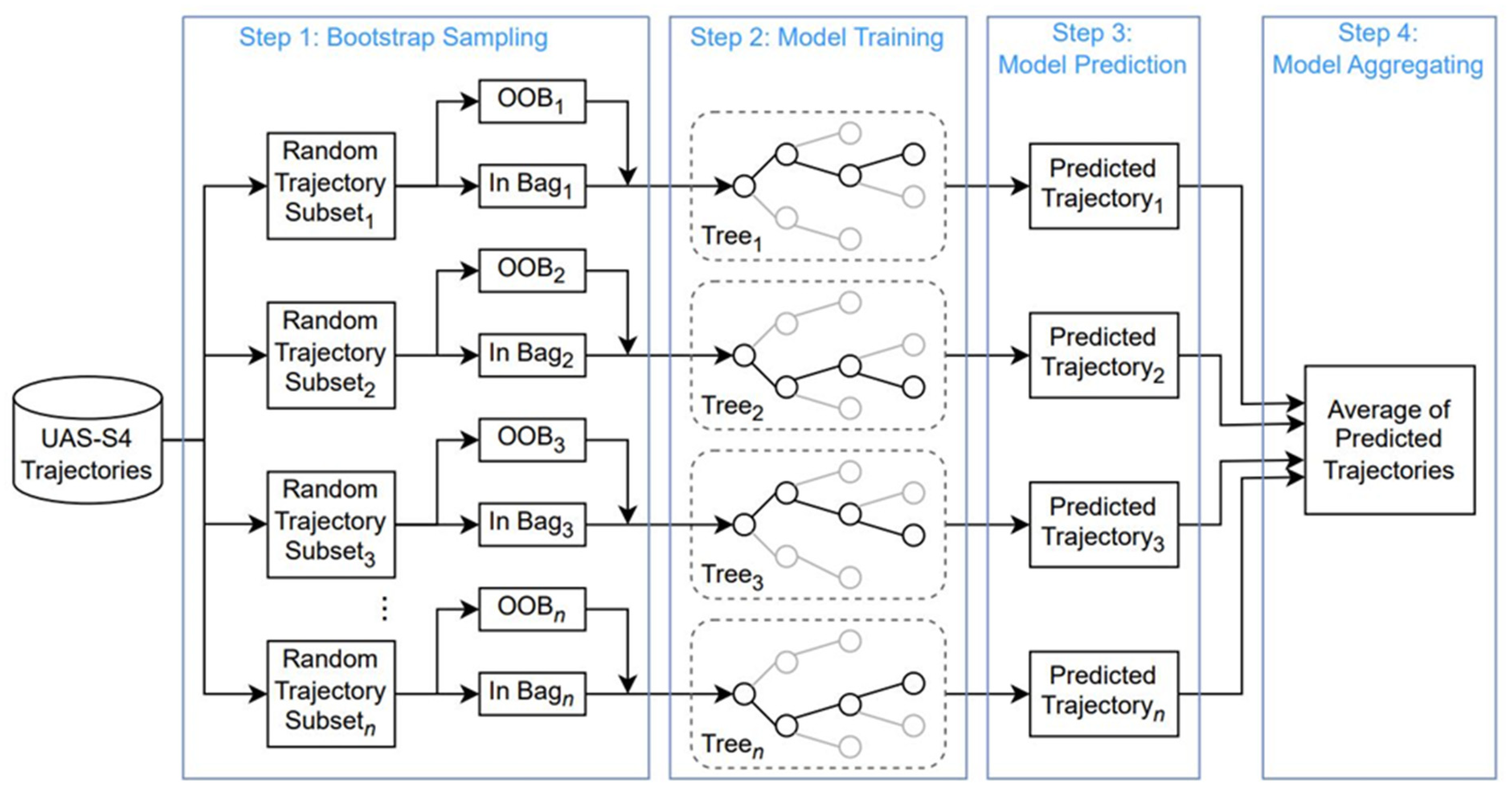
• Model Training: ‘RandomForestRegressor’ was imported from the ‘sklearn.ensemble’ library. The RF model was trained while the out-of-bag (OOB) error was enabled [43]. This error is the average squared difference for regression. The OOB error was monitored during training to provide a preliminary estimate of model performance, in which internal validation (the OOB samples acted as validation sets) and unbiased estimates (since the model was tested on samples it had not seen during training) are provided. Eventually, the RF model learns to make predictions based on the input features and their relationships to the target variable.
• Model Evaluation: After training the RF model, Mean Absolute Percentage Error (MAPE) and out-of-bag (OOB) error were considered as metrics for performance analysis.
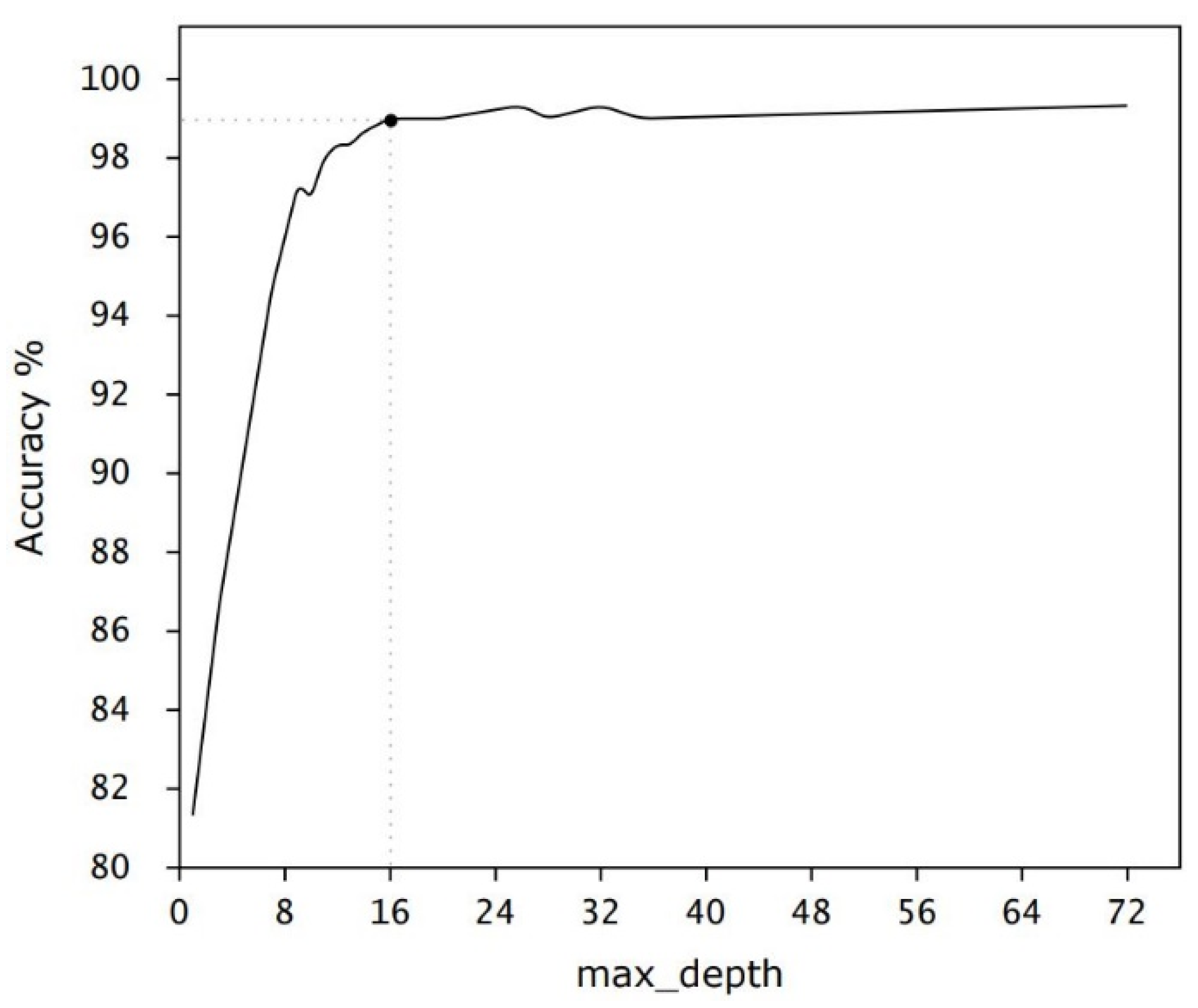
• Model Optimization: The effectiveness of the RF model for trajectory prediction depends on multiple factors, such as data quality and hyperparameter tuning. Fine-tuning of the RF model hyperparameter is necessary to achieve optimal performance. For hyperparameter tuning, parameters including ‘n_estimators’ [44], ‘max_depth’ [45], ‘min_samples_split’, and ‘min_samples_leaf’ [46] were adjusted using ‘GridSearchCV’ to improve performance.
• Real-time Prediction: This process consists of using the trained RF model to make new trajectory predictions. The relevant features are input for each trajectory, and the model outputs predicted future trajectories based on learned patterns. The RF model calculates the average of decisions (predictions made by trees) [47]. The additive model combines decisions from a series of base models using the relationship $g=f_0+f_1+\dots +f_k$. Therefore, the final model g is the sum of base models $f_k$. Figure 2 illustrates the architecture of the RF model with the aim of the UAS-S4 trajectory prediction.

Firstly, trajectory dataset containing the UAS-S4 GPS data provides n trajectory samples for the RF model. These samples are transmitted to the ‘In-Bag’ and ‘Out-of-Bag’ blocks in parallel. The ‘In-Bag’ block provides a subset of training samples used to train a particular decision tree within the ensemble. The ‘Out-of-Bag’ block gathers samples as a subset of training data that are not used during the training of a specific decision tree within the ensemble. Relying on the ‘In-Bag’ and ‘Out-of-Bag’ blocks, the bootstrap sampling process is executed. In this bootstrap sampling, samples are randomly selected and replaced in the original dataset to create a new dataset of equivalent size. On average, approximately 63.3% of the unique instances from the original dataset are selected at least once in this process (known as ‘In-Bag’ samples). The remaining 36.7% that are not selected constitute the OOB samples for that specific tree. Samples are then sent to the trees as a unique regressor and have a particular architecture. Trees are trained, and each makes trajectory predictions based on its individual learning. Predicted trajectories are collected, and their average is considered as the most representative value.

4. Results and Discussion

The Random Forest (RF) method, as a machine learning algorithm, can reach its full capabilities if it accesses to a large and comprehensive dataset. To create such a dataset, the UAS-S4 system was used to generate a significant number of aircraft trajectories, creating a high-quality training database. Figure 3 shows the UAS-S4 Ehécatl manufactured by Hydra Technologies, and

Table 1. The UAS-S4 geometrical and flight data parameters.

Specification	Value
Wingspan	4.2 m
Wing area	2.3 m2
Total length	2.5 m
Mean aerodynamic chord	0.57 m
Empty weight	50 kg
Maximum take-off weight	80 kg
Loitering airspeed	35 knots
Maximum speed	135 knots
Service ceiling	15,000 ft
Operational range	120 km

provides detailed specifications regarding its geometry and flight data parameters.

The flight dynamics of the UAS-S4 were modeled around its equilibrium by analyzing its differential equations for lateral and longitudinal motion [48]. The longitudinal state vector, $X_{lon}={\left[u w q \theta \right]}^T$ was made up of state variables including axial velocity u, vertical velocity w, pitch rate q, and pitch angle $\theta$. This vector is governed by the longitudinal input vector ${\delta }_{lon}={\left[\begin{array}{cc}{\delta }_e& {\delta }_T\end{array}\right]}^T$, comprising elevator deflection ${\delta }_e$ and thrust ${\delta }_T$. Similarly, the lateral state vector, $X_{lat}={\left[v p r \phi \right]}^T$ includes lateral velocity v, roll rate p, yaw rate r, and roll angle $\phi$ and is influenced by the lateral input vector ${\delta }_{lat}={\left[\begin{array}{cc}{\delta }_a& {\delta }_r\end{array}\right]}^T$, which includes aileron and rudder deflections. In any trim condition, the UAS-S4 Flight Dynamics Model (FDM) is representable through a state-space system that employs the state vector $X$, input vector $\delta$, and output vector $Y$ [48].

$$\begin{array}{c}\dot{X}\left(t\right)=A X\left(t\right)+B \delta \left(t\right) \\ Y\left(t\right)=C X\left(t\right)+D \delta \left(t\right) \end{array}$$

(1)

where the matrices for the longitudinal state space are [48]:

$$\begin{array}{l}{A}_{lon}=\left[\begin{array}{cc}\begin{array}{c}{G}_u\\ \begin{array}{c}{H}_u\\ \begin{array}{c}{M}_u+M_{\dot{w}}{H}_u\\ 0\end{array}\end{array}\end{array}& \begin{array}{cc}\begin{array}{c}{G}_w\\ \begin{array}{c}{H}_w\\ \begin{array}{c}{M}_w+M_{\dot{w}}{H}_w\\ 0\end{array}\end{array}\end{array}& \begin{array}{cc}\begin{array}{c}0\\ \begin{array}{c}{u}_0\\ \begin{array}{c}{M}_q+{u_{0}M}_{\dot{w}}\\ 1\end{array}\end{array}\end{array}& \begin{array}{c}{-g}_{ }\mathit{cos}{\theta }_0\\ \begin{array}{c}-g_{ }\mathit{sin}{\theta }_0\\ \begin{array}{c}0\\ 0\end{array}\end{array}\end{array}\end{array}\end{array}\end{array}\right]\\ B_{lon}=\left[\begin{array}{cc}\begin{array}{c}{G}_{{\delta }_e}\\ \begin{array}{c}{H}_{{\delta }_e}\\ \begin{array}{c}{M}_{{\delta }_e}+M_{\dot{w}}{H}_{{\delta }_e}\\ 0\end{array}\end{array}\end{array}& \begin{array}{c}{G}_{{\delta }_T}\\ \begin{array}{c}{H}_{{\delta }_T}\\ \begin{array}{c}{M}_{{\delta }_T}+M_{\dot{w}}{H}_{{\delta }_T}\\ 0\end{array}\end{array}\end{array}\end{array}\right],C_{lon}={\left[\begin{array}{c}0\\ \begin{array}{c}0\\ \begin{array}{c}0\\ 1\end{array}\end{array}\end{array}\right]}^T, D_{lon}=0\end{array}$$

(2)

and the matrices for the lateral state-space include [48]:

$$\begin{array}{l}{A}_{lat}=\left[\begin{array}{cccc}{Y}_v& Y_p& -\left({u_0-Y}_r\right)& g_{ }\mathit{cos}{\theta }_0\\ L_v& L_p& L_r& 0\\ N_v& N_p& N_r& 0\\ 0& 1& 0& 0\end{array}\right]\\ B_{lat}=\left[\begin{array}{cc}\begin{array}{c}0\\ \begin{array}{c}{L}_{{\delta }_a}\\ \begin{array}{c}{N}_{{\delta }_a}\\ 0\end{array}\end{array}\end{array}& \begin{array}{c}{Y}_{{\delta }_r}\\ \begin{array}{c}{L}_{{\delta }_r}\\ \begin{array}{c}{N}_{{\delta }_r}\\ 0\end{array}\end{array}\end{array}\end{array}\right]C_{lat}={\left[\begin{array}{c}0\\ \begin{array}{c}0\\ \begin{array}{c}0\\ 1\end{array}\end{array}\end{array}\right]}^T, D_{lat}=0\end{array}$$

(3)

and $G_u,G_w,H_u,H_w,M_u,M_w,M_q,G_{\delta },H_{\delta },M_{\delta }$ are the longitudinal and $Y_v,Y_p,Y_r,L_v,L_p,L_r,N_v,N_p,N_r,Y_{\delta },L_{\delta },N_{\delta }$ are the lateral dimensional stability derivatives.

The database of aircraft trajectories was generated using a simulator that was developed using our UAS-S4 flight dynamics model, which incorporates a support vector regression (SVR) algorithm [49,50] and a resilient adaptive fuzzy controller [48]. This database includes 1820 trajectories that contain 218,400 samples. Each sample is represented as a vector as [latitude, longitude, altitude, heading, speed, time] T obtained from the GPS data.

In the literature review section, both the Linear Regression (LR) and Long Short-Term Memory (LSTM) models were considered for comparison with the Random Forest (RF) method. The Random Forest (RF) model was trained using the UAS-S4 trajectory dataset. Subsequently, its performance was benchmarked versus that of the LR and LSTM models, as this comparison primarily focused on the Mean Absolute Percentage Error (MAPE) as an evaluation metric, which is not highly sensitive to outliers [51]. Outliers refer to data points that deviate significantly from the other observations, potentially due to variability or errors. They can influence the outcome of statistical analyses and might sometimes lead to misleading conclusions.

The MAPE is a metric used to evaluate the performance of regression models. It provides a straightforward way to calculate the average error of predictions, whether the error is due to underestimation or overestimation, which can be represented in Equation (4):

$$\mathrm{M}\mathrm{A}\mathrm{P}\mathrm{E}=\frac{1}{m} {\sum }_{j=1}^m\left| \frac{y_i-{\widehat{y}}_i}{y_i}\ast 100 \right|$$

(4)

where m is the total number of observations, $y_i$ is the actual values, and ${\widehat{y}}_i$is the predicted values including latitude, longitude, altitude, heading, speed, and time. The error was computed based on measuring Euclidean distance. Since for specific altitudes, UAS-S4s were arranged in a 16 km² flight zone, and each sector was 100 m × 100 m, 1% error could be 1.4 m at max [4]. By considering 1.4 m misplacement for 1% error, the MAPE can give a more comprehensible result.

The calculation expressed by Equation (1) involves subtracting each predicted value from its corresponding actual value by taking the absolute value of each of these differences and then by averaging these absolute differences over a number of observations. The resultant value, expressed in units of the predicted variable, provides a straightforward indication of the average magnitude of the prediction errors, regardless of their direction. A lower MAPE indicates that a model is more accurate, while a higher MAPE suggests that the predictions are, on average, farther from their actual values. Figure 4 provides an insight into the performance of various prediction models by using the Mean Absolute Percentage Error (MAPE) index as the evaluation metric.

In Figure 4, MAPE values are depicted for the LR, LSTM, and RF models used for trajectory prediction. The LSTM and LR models are those of the designed models in our previous study [25]. Each model was assessed within a prediction horizon spanning 5 min. The LR model could never surpass the performance levels exhibited by its counterparts, LSTM and RF, and its lowest MAPE (1.19%) was achieved for the immediate prediction. The error was computed based on measuring Euclidean distance. Since, for specific altitudes, UAS-S4s were arranged in a 16 km² flight zone, and each sector was 100 m × 100 m, 1% error could be 1.4 m at max [4].

In the short-term prediction window spanning 1 to 2 min, the RF model outperformed both the LSTM and LR, with an average MAPE that was 0.23% lower. However, for long-term predictions within a 4 to 5 min horizon, LSTM was better than the RF model by an average of 0.31% MAPE reduction. For the specific task of evaluating available airspaces for UAV allocation, which requires a maximum prediction horizon of 2 min, the RF model is more efficient than the LSTM for its predictive performance. Additionally, for our UAS-S4 trajectory dataset, training of the RF model was 2.7 times faster than the LSTM (using two GTX TITAN X GPUs). The RF had a simpler mechanism for avoiding overfitting. As a result, we opted for the RF model for predicting UAS-S4 trajectories. The trained RF model could predict the UAS-S4 trajectories over a 2 min horizon in no longer than 69 ms.

Given the very good performance of the RF model, it is needed to optimize its hyperparameters. In this way, the OOB error was used for evaluating the ‘min_sample_leaf’, and ‘min_sample_split’ hyperparameters as it offered a reliable estimate of the RF model performance on unseen data. It was crucial for determining the optimal minimum number of samples per leaf and split to prevent overfitting. The OOB error was calculated using the following procedure.

i.

For each training instance (data point) that was not included in the bootstrap sample (i.e., left out of the bag) for a particular tree in the ensemble, its value was predicted using that tree.

ii.

After all trees are constructed, for each training instance, the average of the predictions made by the trees for which that instance was out-of-bag was calculated.

iii.

The OOB error is then the average of the squared differences between these averaged predictions and the actual values of the training instances. Mathematically, if $y_i$ is the actual value of the i^th instance and ${\widehat{y}}_i$ is the averaged OOB prediction for that instance, then the OOB error is calculated as:

$$\mathrm{O}\mathrm{O}\mathrm{B} error=\frac{1}{n} \sum _{i=1}^n{(y_i-{\widehat{y}}_i)}^2$$

(5)

where $n$ is the number of training instances.

While normalization of input features is not essential for Random Forest models due to their inherent scale invariance, it does not harm the model’s performance and leads to some side benefits such as uniformity, outlier sensitivity, and consistency with other models. We normalized the RF’s input features, especially for its consistency across different models. This is essential for our further transferability analysis of adversarial attacks. Input feature normalization caused $(y-\widehat{y})$ ranges between 0 and 1 and consequently, in Equation (5), OOB error ∈ [0, 1].

We determined accuracy for evaluating the ‘max_depth’ hyperparameter as it could provide a straightforward measure of overall RF model performance regarding the balanced UAS-S4 dataset. Accuracy was calculated as the percentage that complements the out-of-bag (OOB) error.

$$accuracy=(1-\mathrm{O}\mathrm{O}\mathrm{B} error)\times 100$$

(6)

Following the hyperparameter tuning, the ‘max_features’ hyperparameter controls the number of features that should be considered when looking for the best split at each node in the decision tree. The most common settings for ‘max_features’ in a regression problem are ‘None’, ‘log2’, and ‘sqrt’. ‘None’ considers all the features for finding the best split at each node; ‘log2’ uses log2 of the number of features, which means that a very small subset of features is considered at each split, which may be useful for very high-dimensional datasets; and ‘sqrt’ uses the square root of the number of features for making the best split at each node. It is often used as a default heuristic by providing a good balance between creating diverse trees and the depth of trees. The aim is to balance between model diversity (having different trees in a forest may capture different patterns) and the prediction accuracy of individual trees. We used OOB error to evaluate the RF performance using various ‘max_features’.

Figure 5 depicts the RF model performance in terms of an OOB error percentage (%) for different ‘max_features’ settings.

Figure 5 illustrates a graph where the x-axis represents the number of estimators and the y-axis depicts the out-of-bag (OOB) error. In this figure, three ‘line’ and ‘dot’ styles are present: a dashed line corresponding to ‘max_features’ set as ‘None’, a solid line for the ‘sqrt’ setting, and a dotted line associated with ‘log2’. It is noticeable from the graph that as the number of trees reaches 14, the OOB error for RFs begins to stabilize. By analyzing the results more closely, it was found that the ‘sqrt’ setting provided the smallest rate of out-of-bag error, whereas the log2 setting demonstrated enhanced precision in the validation accuracy. In other words, the out-of-bag error did not vary significantly as the number of trees increased.

‘max_depth’ is a crucial hyperparameter used in the RF model and other tree-based algorithms such as decision trees and gradient boosting trees. The ‘max_depth’ parameter specifies the maximum depth of each tree in the Random Forest. The depth of a tree is the maximum distance from the root node to any leaf node. This hyperparameter is supposed to control overfitting, model complexity, and training time. By limiting the depth of the trees, the model can avoid fitting too closely to the training data, thus helping to mitigate overfitting. Deeper trees can model more complex patterns, but they may also capture noise in the data. Shallower trees can generally train the model faster than the deeper trees because there are fewer computations to perform. Figure 6 illustrates the RF accuracy for a variety of ‘max_depth’ values. Setting an appropriate ‘max_depth’ helps manage the trade-off between model complexity and overfitting.

Given that trajectory data comprise a limited set of features, our evaluation primarily zeroes in on the test data accuracy, taking into account variations in forest size and the maximal depth of individual trees. As depicted in Figure 6, a direct correlation exists between an enlarged number of trees in the forest and enhanced accuracy of the RF model. The RF model accuracy increases with the ‘max_depth’ value. Specifically, the accuracy experiences a growth with each additional tree introduced, eventually stabilizing once the count reaches 16 trees (black point). A close examination of Figure 6 reveals that the maximum accuracy was achieved using the RF model when it reached 99.4% with 28 trees. We utilized 16 trees in order to avoid overfitting and model complexity.

A very deep tree might capture noise in the data and overfit, while a very shallow tree might not be able to capture the underlying patterns, resulting in underfitting. Other regularization hyperparameters in tandem with ‘max_depth’, such as ‘min_samples_split’ and ‘min_samples_leaf’, can be considered. These hyperparameters were involved in the proposed RF trajectory prediction model. They help to control the growth of the trees and, consequently, affect the model performance and complexity. ‘min_samples_split’ defines the minimum number of samples required to split an internal node. Figure 7 shows the OOB error obtained in % for various ‘min_samples_split’ values.

By considering ‘max_features’ = 14 and ‘max_depth’ = 16, setting the ‘min_samples_split’ value higher can smooth the RF model, resulting in less overfitting. A higher value of ‘min_samples_split’ means that our RF algorithm is less likely to learn fine-grained UAS-S4 trajectory patterns, which could result in a simpler model. On the other hand, with fewer splits, the RF model is less flexible and cannot adequately capture the underlying patterns in the data, leading to higher bias and underfitting. Moreover, the RF model becomes less sensitive to variations in the data. While this fact might reduce overfitting, it also prevents the RF model from learning important, finer-grained UAS-S4 trajectory patterns that are crucial for accurate predictions.

The other pivotal hyperparameter is ‘min_samples_leaf’, which specifies the minimum number of samples required at a leaf node. Setting this to a high value creates a constraint on refining the partitions, which smoothens the model and avoids overfitting. With a larger number of samples in the leaf, the model becomes more robust to noise in the data. Figure 8 shows the RF model performance in terms of OOB error with increasing ‘min_samples_leaf’.

Utilizing ‘max_features’ = 14, ‘max_depth’ = 16, and higher values for the ‘min_samples_leaf’ parameter prevents the RF model from overfitting, but excessive values might lead to model overfitting. On the other hand, the RF model trained with a low ‘min_samples_leaf’ value might not generalize well to new data because it is too tailored to the training data and can result in lower accuracy. These parameters should be adjusted using techniques such as grid search, random search, or Bayesian optimization. The proper tuning of these hyperparameters generalizes the RF model well to unseen data by effectively balancing bias and variance. For the RF model, the ‘min_samples_split’ was considered 9 where the OOB error was 1.13%, and ‘min_samples_leaf’ was set into 10 where the OOB error was 1.28% using the ‘GridSearchCV’ optimizer. This optimizer in the Scikit-learn library facilitates hyperparameter optimization by exhaustively evaluating model performance across a defined parameter grid. Using cross-validation, it assesses every parameter combination, typically employing metrics such as accuracy or precision to determine the best configuration. Upon identifying the optimal parameters, the model is trained on the complete dataset. Using the UAS-S4 dataset, the RF model was trained, and its hyperparameters were tuned accordingly. The optimized RF model accurately predicted the future trajectories of the UAS-S4.

5. Conclusions

This study provides a comprehensive analysis to evaluate the efficiency of the Random Forest (RF) methodology in predicting aircraft trajectories. In this study, the RF approach was compared to two renowned data-driven models: Long Short-Term Memory (LSTM) and Logistic Regression (LR). The research relies on a considerable dataset comprising historical aircraft trajectory data obtained from a UAS-S4 simulator.

The study shows that, within the constraint of a short-term prediction horizon, the RF methodology excels in trajectory prediction accuracy, outshining both the LSTM and LR models. Furthermore, a meticulous optimization process was undertaken to enhance the RF methodology performance, which involved fine-tuning several hyperparameters, including the number of estimators, features, depth, split, and leaf parameters.

Notably, it was observed that selecting ‘max_feature’ = sqrt yielded the lowest rate of out-of-bag error for the RF under stable conditions. The model accuracy saw substantial improvement with the addition of each tree. Increasing the ‘min_samples_split’ value induced a smoothing effect on the model, consequently mitigating the risk of overfitting. In essence, a higher ‘min_samples_split’ value restrained the algorithm from learning overly detailed patterns, culminating in a model with a simplified structure. Similarly, increasing the ‘min_samples_leaf’ value imposed restrictions on further partition refinements, ensuring the model remained smooth and resilient to overfitting. When the leaf nodes had a higher sample count, the model demonstrated enhanced robustness against data noise. Together, these insights underscored the promising potential of the RF methodology, highlighting it as a valuable alternative to the LSTM and LR models, particularly in tasks requiring short-term trajectory prediction.

References

1. Ghommam, J.; Saad, M.; Mnif, F.; Zhu, Q.M. Guaranteed performance design for formation tracking and collision avoidance of multiple USVs with disturbances and unmodeled dynamics. IEEE Syst. J. 2020, 15, 4346–4357. [Google Scholar] [CrossRef]
2. Ollero, A.; Maza, I. Multiple Heterogeneous Unmanned Aerial Vehicles; Springer: Berlin/Heidelberg, Germany, 2007; Volume 37. [Google Scholar]
3. Hashemi, S.M. Novel Trajectory Prediction and Flight Dynamics Modelling and Control Based on Robust Artificial Intelligence Algorithms for the UAS-S4; École de Technologie Supérieure: Montreal, QC, Canada, 2022. [Google Scholar]
4. Hashemi, S.; Botez, R.M.; Ghazi, G. Comparison Study between PoW and PoS Blockchains for Unmanned Aircraft System Traffic Management. In Proceedings of the AIAA AVIATION 2023 Forum, San Diego, CA, USA, 12–16 June 2023. [Google Scholar]
5. Ghazi, G.; Botez, R.M.; Domanti, S. New methodology for aircraft performance model identification for flight management system applications. J. Aerosp. Inf. Syst. 2020, 17, 294–310. [Google Scholar] [CrossRef]
6. Cestino, D.; Crosasso, P.; Rapellino, M.; Cestino, E.; Frulla, G. Safety assessment of pharmaceutical distribution in a hospital environment. J. Healthc. Technol. Manag. 2013, 1, 10–21. [Google Scholar] [CrossRef]
7. Izadi, H.; Gordon, B.; Zhang, Y. Safe path planning in the presence of large communication delays using tube model predictive control. In Proceedings of the AIAA Guidance, Navigation, and Control Conference, Toronto, ON, Canada, 2–5 August 2010. [Google Scholar]
8. Zhou, X.; Yu, X.; Guo, K.; Zhou, S.; Guo, L.; Zhang, Y.; Peng, X. Safety flight control design of a quadrotor UAV with capability analysis. IEEE Trans. Cybern. 2021, 53, 1738–1751. [Google Scholar]
9. Ghazi, G.; Botez, R.M. Identification and validation of an engine performance database model for the flight management system. J. Aerosp. Inf. Syst. 2019, 16, 307–326. [Google Scholar] [CrossRef]
10. Ghommam, J.; Rahman, M.H.; Saad, M. Design of distributed event-triggered circumnavigation control of a moving target by a group of underactuated surface vessels. Eur. J. Control. 2022, 67, 100702. [Google Scholar] [CrossRef]
11. Tuzcu, I.; Marzocca, P.; Cestino, E.; Romeo, G.; Frulla, G. Stability and control of a high-altitude, long-endurance UAV. J. Guid. Control Dyn. 2007, 30, 713–721. [Google Scholar] [CrossRef]
12. Ghommam, J.; Saad, M.; Wright, S.; Zhu, Q.M. Relay manoeuvre based fixed-time synchronized tracking control for UAV transport system. Aerosp. Sci. Technol. 2020, 103, 105887. [Google Scholar] [CrossRef]
13. Romeo, G.; Cestino, E.; Borello, F.; Pacino, M. Very-Long Endurance Solar Powered Autonomous UAVs: Role and Constraints for GMEs Applications. In Proceedings of the 28th International Congress of the Aeronautical Sciences–ICAS, Brisbane, Australia, 23–28 September 2012. [Google Scholar]
14. Zhou, X.; Yu, X.; Zhang, Y.; Luo, Y.; Peng, X. Trajectory planning and tracking strategy applied to an unmanned ground vehicle in the presence of obstacles. IEEE Trans. Autom. Sci. Eng. 2020, 18, 1575–1589. [Google Scholar] [CrossRef]
15. Hashemi, S.M.; Hashemi, S.A.; Botez, R.M. Reliable Aircraft Trajectory Prediction Using Autoencoder Secured with P2P Blockchain. In International Symposium on Unmanned Systems and The Defense Industry; Springer: Berlin/Heidelberg, Germany, 2022. [Google Scholar]
16. Ghazi, G.; Gerardin, B.; Gelhaye, M.; Botez, R.M. New adaptive algorithm development for monitoring aircraft performance and improving flight management system predictions. J. Aerosp. Inf. Syst. 2020, 17, 97–112. [Google Scholar] [CrossRef]
17. Di Gravio, G.; Mancini, M.; Patriarca, R.; Costantino, F. Overall safety performance of Air Traffic Management system: Forecasting and monitoring. Saf. Sci. 2015, 72, 351–362. [Google Scholar] [CrossRef]
18. Mennequin, A.; Ghazi, G.; Botez, R.M. Cessna Citation X aircraft trajectory prediction using an aero-propulsive model. In Proceedings of the Poster Presented at the Conference: 6th Edition of the Montreal Innovation Summit (SMI), Montreal, QC, Canada, 24 November 2016. [Google Scholar]
19. Prevost, C.G.; Desbiens, A.; Gagnon, E. Extended Kalman filter for state estimation and trajectory prediction of a moving object detected by an unmanned aerial vehicle. In Proceedings of the 2007 American Control Conference, New York, NY, USA, 9–13 July 2007; IEEE: Piscataway, NJ, USA, 2007. [Google Scholar]
20. Yang, X.; Sun, J.; Rajan, R.T. Aircraft Trajectory Prediction using ADS-B Data. In Proceedings of the Pre-Proceedings of the 2022 Symposium on Information Theory and Signal Processing in the Benelux, Louvain la Neuve, Belgium, 1–2 June 2022. [Google Scholar]
21. Khedmati, M.; Seifi, F.; Azizi, M. Time series forecasting of bitcoin price based on autoregressive integrated moving average and machine learning approaches. Int. J. Eng. 2020, 33, 1293–1303. [Google Scholar]
22. Xing, Y.; Wang, G.; Zhu, Y. Application of an autoregressive moving average approach in flight trajectory simulation. In Proceedings of the AIAA Atmospheric Flight Mechanics Conference, Washington, DC, USA, 13–17 June 2016. [Google Scholar]
23. Pang, Y.; Yao, H.; Hu, J.; Liu, Y. A recurrent neural network approach for aircraft trajectory prediction with weather features from sherlock. In Proceedings of the AIAA Aviation 2019 Forum, Dallas, TX, USA, 17–21 June 2019. [Google Scholar]
24. Hashemi, S.M.; Hashemi, S.A.; Botez, R.M.; Ghazi, G. Aircraft Trajectory Prediction Enhanced through Resilient Generative Adversarial Networks Secured by Blockchain: Application to UAS-S4 Ehécatl. Appl. Sci. 2023, 13, 9503. [Google Scholar] [CrossRef]
25. Hashemi, S.M.; Botez, R.M.; Grigorie, T.L. New reliability studies of data-driven aircraft trajectory prediction. Aerospace 2020, 7, 145. [Google Scholar] [CrossRef]
26. Pang, Y.; Zhao, X.; Yan, H.; Liu, Y. Data-driven trajectory prediction with weather uncertainties: A Bayesian deep learning approach. Transp. Res. Part C Emerg. Technol. 2021, 130, 103326. [Google Scholar] [CrossRef]
27. Hashemi, S.M.; Hashemi, S.A.; Botez, R.M.; Ghazi, G. A novel fault-tolerant air traffic management methodology using autoencoder and P2P blockchain consensus protocol. Aerospace 2023, 10, 357. [Google Scholar] [CrossRef]
28. Wang, Z.; Liang, M.; Delahaye, D. Automated data-driven prediction on aircraft Estimated Time of Arrival. J. Air Transp. Manag. 2020, 88, 101840. [Google Scholar] [CrossRef]
29. Sagi, O.; Rokach, L. Ensemble learning: A survey. Wiley Interdiscip. Rev. Data Min. Knowl. Discov. 2018, 8, e1249. [Google Scholar] [CrossRef]
30. Zhang, C.; Ma, Y. Ensemble Machine Learning: Methods and Applications; Springer: Berlin/Heidelberg, Germany, 2012. [Google Scholar]
31. Hashemi, S.; Hashemi, S.A.; Botez, R.M.; Ghazi, G. Attack-tolerant Trajectory Prediction using Generative Adversarial Network Secured by Blockchain Application to the UAS-S4 Ehécatl. In Proceedings of the AIAA SCITECH 2023 Forum, National Harbor, MD, USA, 23–27 January 2023. [Google Scholar]
32. Hashemi, S.; Hashemi, S.A.; Botez, R.M.; Ghazi, G. A Novel Air Traffic Management and Control Methodology using Fault-Tolerant Autoencoder and P2P Blockchain Application on the UAS-S4 Ehécatl. In Proceedings of the AIAA SCITECH 2023 Forum, National Harbor, MD, USA, 23–27 January 2023. [Google Scholar]
33. Kokalj-Filipovic, S.; Miller, R. Adversarial examples in RF deep learning: Detection of the attack and its physical robustness. arXiv 2019, arXiv:1902.06044. [Google Scholar]
34. Guo, Z.; Yu, B.; Hao, M.; Wang, W.; Jiang, Y.; Zong, F. A novel hybrid method for flight departure delay prediction using Random Forest Regression and Maximal Information Coefficient. Aerosp. Sci. Technol. 2021, 116, 106822. [Google Scholar] [CrossRef]
35. Heaton, J. An empirical analysis of feature engineering for predictive modeling. In Proceedings of the SoutheastCon 2016, Norfolk, VA, USA, 30 March–3 April 2016; IEEE: Piscataway, NJ, USA, 2016. [Google Scholar]
36. Majda, A.J.; Harlim, J. Physics constrained nonlinear regression models for time series. Nonlinearity 2012, 26, 201. [Google Scholar] [CrossRef]
37. Wang, H.; Yao, R.; Hou, L.; Zhao, J.; Zhao, X. A Methodology for Calculating the Contribution of Exogenous Variables to ARIMAX Predictions. In Proceedings of the Canadian Conference on AI, Vancouver, BC, USA, 25–28 May 2021. [Google Scholar]
38. Subramanian, J.; Simon, R. Overfitting in prediction models–is it a problem only in high dimensions? Contemp. Clin. Trials 2013, 36, 636–641. [Google Scholar] [CrossRef] [PubMed]
39. Kernbach, J.M.; Staartjes, V.E. Foundations of machine learning-based clinical prediction modeling: Part II—Generalization and overfitting. In Machine Learning in Clinical Neuroscience: Foundations and Applications; Springer: Berlin/Heidelberg, Germany, 2022; pp. 15–21. [Google Scholar]
40. Cheng, J.C.; Chen, W.; Chen, K.; Wang, Q. Data-driven predictive maintenance planning framework for MEP components based on BIM and IoT using machine learning algorithms. Autom. Constr. 2020, 112, 103087. [Google Scholar] [CrossRef]
41. Biau, G.; Scornet, E. A random forest guided tour. Test 2016, 25, 197–227. [Google Scholar] [CrossRef]
42. Khurana, U.; Samulowitz, H.; Turaga, D. Feature engineering for predictive modeling using reinforcement learning. In Proceedings of the Proceedings of the AAAI Conference on Artificial Intelligence, New Orleans, LA, USA, 2–7 February 2018. [Google Scholar]
43. Janitza, S.; Hornung, R. On the overestimation of random forest’s out-of-bag error. PLoS ONE 2018, 13, e0201904. [Google Scholar] [CrossRef]
44. Probst, P.; Boulesteix, A.-L. To tune or not to tune the number of trees in random forest. J. Mach. Learn. Res. 2017, 18, 6673–6690. [Google Scholar]
45. Nadi, A.; Moradi, H. Increasing the views and reducing the depth in random forest. Expert Syst. Appl. 2019, 138, 112801. [Google Scholar] [CrossRef]
46. Lee, T.-H.; Ullah, A.; Wang, R. Bootstrap aggregating and random forest. In Macroeconomic Forecasting in the Era of Big Data: Theory and Practice; Springer: Berlin/Heidelberg, Germany, 2020; pp. 389–429. [Google Scholar]
47. Gossen, F.; Steffen, B. Algebraic aggregation of random forests: Towards explainability and rapid evaluation. Int. J. Softw. Tools Technol. Transf. 2021, 25, 267–285. [Google Scholar] [CrossRef]
48. Hashemi, S.; Botez, R.M. Lyapunov-based robust adaptive configuration of the UAS-S4 flight dynamics fuzzy controller. Aeronaut. J. 2022, 126, 1187–1209. [Google Scholar] [CrossRef]
49. Hashemi, S.M.; Botez, R.M. A Novel Flight Dynamics Modeling Using Robust Support Vector Regression against Adversarial Attacks. SAE Int. J. Aerosp. 2023, 16, 305–323. [Google Scholar] [CrossRef]
50. Hashemi, S.M.; Botez, R.M. Support vector regression application for the flight dynamics new modelling of the UAS-S4. In Proceedings of the AIAA SCITECH 2022 Forum, San Diego, CA, USA, 3–7 January 2022. [Google Scholar]
51. De Myttenaere, A.; Golden, B.; Le Grand, B.; Rossi, F. Mean absolute percentage error for regression models. Neurocomputing 2016, 192, 38–48. [Google Scholar] [CrossRef]
Figure 1. Sequential aircraft trajectory prediction [27].
Aerospace 11 00049 g001
Figure 2. Random Forest (RF) architecture for trajectory prediction.
Aerospace 11 00049 g002
Figure 3. Hydra Technologies UAS-S4 Ehécatl.
Aerospace 11 00049 g003
Figure 4. Prediction performance using the LR, LSTM, and RF models.
Aerospace 11 00049 g004
Figure 5. The RF performance using different ‘max_features’.
Aerospace 11 00049 g005
Figure 6. The RF accuracy for different ‘max_depth’ hyperparameter values.
Aerospace 11 00049 g006
Figure 7. Out-of-bag (OOB) error versus ‘min_samples_split’.
Aerospace 11 00049 g007
Figure 8. Out-of-bag (OOB) error versus ‘min_samples_leaf’.
Aerospace 11 00049 g008