Article

Airfoil Lift Coefficient Optimization Using Genetic Algorithm and IGP Parameterization: Volume 1

by
María Elena Tejeda-del-Cueto
1,2,
Manuel Alberto Flores-Alfaro
1,
Miguel Toledo-Velázquez
3,
Lorena del Carmen Santos-Cortes
1,
José Hernández-Hernández
1,2 and
Marco Osvaldo Vigueras-Zúñiga
1,2,*
1
Faculty of Engineering of the Construction and Habitat, Universidad Veracruzana, Veracruz 94299, Mexico
2
Mechanical Engineering Department, Universidad Veracruzana, Veracruz 94294, Mexico
3
Laboratorio de Ingeniería Térmica e Hidráulica Aplicada (LABINTHAP), IPN-ESIME Zacatenco, Mexico City 07738, Mexico
*
Author to whom correspondence should be addressed.
Aerospace 2024, 11(1), 44; https://doi.org/10.3390/aerospace11010044
Submission received: 5 November 2023 / Revised: 18 December 2023 / Accepted: 29 December 2023 / Published: 30 December 2023

Abstract

:
The objective of this study is to develop a genetic algorithm that uses the IGP parameterization to increase the lift coefficient (CL) of three airfoils to be used on wings of unmanned aerial vehicles (UAVs). The geometry of three baseline airfoils was modified by developing a genetic algorithm that operates with the IGP parameterization and performs the aerodynamic analysis using XFOIL in the MATLAB environment. Subsequently, a numerical model was made for each baseline and optimized airfoil using a commercial computational fluid dynamics (CFD) code to analyze the behavior of the lift coefficient. An increase in the average CL was obtained for the Eppler 68, MH 70, and Wortmann FX 60-126 airfoils for angles of attack ranging from 0 to 10, obtaining increments of 17.243%, 14.967%, and 10.708%, respectively. Additionally, an average 5.027% uncertainty was obtained in lift coefficient calculations between XFOIL and CFD. The utility of the IGP method and genetic algorithms for parameterizing and optimizing airfoils was demonstrated. In addition, airfoils could be tailored for a specific UAV depending on the mission profile. Volume 2 of this study will include experimental data from wind tunnel.

1. Introduction

Nowadays, new and complex aircraft configurations in addition to design methodologies for aerodynamic surfaces enhance the development of customized wings for a required mission profile. Due to the multiple applications of UAVs, researchers focus on the design and development of the wings, as they highly contribute to the performance of UAVs.
An airfoil influences cruise speed, takeoff and landing distances, stall speed, maneuvering capabilities, and overall aerodynamic efficiency during all phases of flight [1]. Given that the performance of an airfoil depends on the Reynolds number in which it operates, the selection of the airfoil according to the application in which it is used is a fundamental aspect of any aircraft design. When considering all possible airfoil design permutations, it becomes apparent that the number of unique sets of requirements exceeds the collection of existing airfoils in databases. For this reason, the advancement and use of airfoil design methods is an attractive solution [2].
Optimization algorithms could usually fall within two categories: gradient-based and heuristic/metaheuristic algorithms. Gradient-based methods have a fast convergence; however, in practice, they could potentially not converge to global optima, being necessary to precisely check their initial conditions to assure some certainty in the optimization process. Comparatively, heuristic/metaheuristic algorithms have a slower convergence and are more reliable and robust, even though convergence is not proven [3]. According to [4], metaheuristic algorithms are divided in two main categories, the single-solution based and the population based; they provide the solution to avoid local optima by using a set of multiple candidate solutions during the optimization process. The most common population-based metaheuristic algorithms are genetic algorithm (GA), particle swarm optimization (PSO) [5,6,7], ant colony optimization (ACO), spotted hyena optimizer (SHO), emperor penguin optimizer (EPO), and seagull optimization algorithm (SOA). Genetic algorithms were first proposed by Holland [8], and according to [9], they have been widely used by researchers in the field of aeronautics as they are efficient in determining the global optimum of the objective function and do not require derivatives. These features make genetic algorithms attractive for practical engineering applications such as shape optimization. During studies conducted by [10,11,12,13,14], genetic algorithms were used for airfoil design, obtaining the maximization of lift and efficiency or the minimization of drag, which are the main features that researchers currently optimize [15].
Airfoil design approaches could be categorized in two main branches, the direct design approach and the inverse design approach [16]. Direct design focuses on developing airfoils based on design rules and then modify their shape based on the momentum, vortex, and cascade method, the panel method, or the CFD method. Panel and CFD methods could use parametric optimization that is based on a set of variables that define airfoil shape that is fully related to its performance to be evaluated through any of the two aforementioned methods. Among the most widely used parametric descriptions are the Hicks–Henne bump functions, B-spline, PARSEC, CST [17], functions of [18] and [19], and recently the improved geometric parameter (IGP) method [20]. Given that IGP is a method where design parameters have a geometric meaning, as seen in PARSEC, it is useful for optimization processes, given it allows designers to directly manipulate the shape of the airfoil instead of using polynomial coefficients [21]. PARSEC is the most widely used parametric method in this field of research; it uses eleven geometric parameters for constructing airfoils. Comparatively, IGP uses eight, thereby reducing the computational cost during airfoil optimization.
One of the main fields of study in airfoil optimization has been performed on turbines where various tools are combined such as geometric parameterization, genetic algorithms, and CFD [22,23,24,25,26]. Another application for the combination of the aforementioned tools is the development of UAVs, which represents one of the most relevant emerging technologies of the last two decades. Construction and infrastructure monitoring, precision agriculture, indoor search and rescue, and of course military are just a few examples of applications for UAVs. They have become a popular instrument for a wide range of applications and have replaced other platforms due to their flexibility and moderate costs, creating new business opportunities [27].
There are tools for airfoil analysis such as XFOIL, which is a solver that uses the panel method. XFOIL has been used successfully in studies by [28,29,30]. XFOIL can provide sufficient precision for the conceptual design phase of airfoils; however, the option of aerodynamic analysis with Navier–Stokes solvers is of significant importance for further detailed design used in CFD. This is applicable not only for two-dimensional steady-state calculations but also for three-dimensional and transient cases [31,32].
The present study proposes to modify the geometry of three existing baseline airfoils by developing a genetic algorithm based on the new IGP parameterization method. The aerodynamic analysis will be performed using XFOIL in the MATLAB environment, and the results will be compared with a corresponding CFD analysis. The outcome will be a set of redesigned airfoils that have an improved lift performance, in the range of turbulence for UAVs specified by Reynolds numbers. This will be the basis for further development that is not dependent on the airfoils found in databases and for generating new geometries that meet the aerodynamic characteristics for the required application.
Motivation for this study was to share knowledge with readers regarding a methodology for designing optimized airfoils tailored to be used on the wings of small tactical UAVs. This study also contributes to the proof of convergence of the GA with the novel IGP parameterization through an automated process between MATLAB and XFOIL. To validate the numerical model of the baseline airfoil, a comparison with experimental data of the FX-60-126 airfoil at Re = 700,000 is presented. Future work will deal with the validation of optimized airfoils through wind tunnel testing. As a result, potentially, any existing airfoil could be optimized to improve its performance using a parametric direct design approach.

2. Optimization Process

2.1. Preliminaries

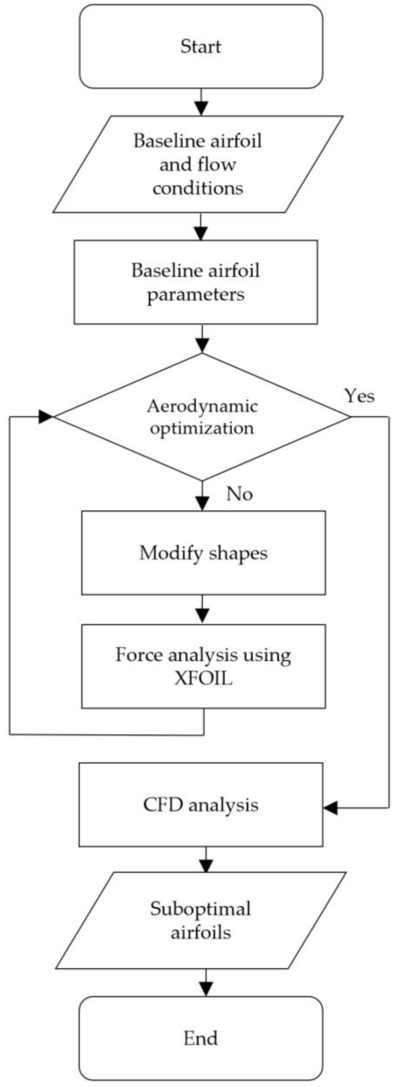
The optimization methodology used in the present study is shown in Figure 1.
To obtain an estimate of Reynolds numbers for the optimization of the airfoils, the information available online from specification sheets of a set of well-known COTS UAVs relevant within the industry was taken, as seen in Table 1. The parameterization and optimization of the airfoils was performed in the MATLAB environment. Reynolds number to perform aerodynamic analysis was obtained by averaging mean aerodynamic chords of UAVs of Table 1 operating with an indicated airspeed of 22 m/s at sea level conditions, resulting in a Reynolds number of 225,964.226, a Mach number of 0.06465, and angles of attack ranging from 0° to 10°.
The Airfoil Tools [33] database was used to compare airfoil performance regarding CL and CD in the computed range of Reynolds numbers. IGP method [20] was applied to a database with a great number of airfoils performing both geometric fitting and aerodynamic verification. In order to validate application of the optimization process in different families of airfoils, three families were selected, and one element of each family was taken. Among airfoils of each family, one member per family was selected considering the ones with the maximum CL in order to improve that parameter as a proof of the optimization methodology. The airfoils selected were the Eppler 68, MH 70 and Wortmann FX 60-126.

2.2. Geometric Description with IGP

In this study, parameterization was performed with the IGP method, which considers Bézier curves as basic functions to describe the camber line of the airfoil, and the polynomial function for the “four-digit” NACA series to describe the thickness. In Equation (1), c 1 and c 2 are the horizontal coordinates of the two control points of the cubic Bézier curves, while c 3 and c 4 in Equation (2) are the vertical coordinates of the two control points of the cubic Bézier curves. k is an independent parameter ranging from 0 to 1 and helps in generating curves.
x c = 3 c 1 k ( 1 k ) 2 + 3 c 2 1 k k 2 + k 3
y c = 3 c 3 k ( 1 k ) 2 + 3 c 4 ( 1 k ) k 2
From the basis function of the thickness curves for the NACA “four-digit” series, the thickness expression is determined in Equation (3).
t = t 1 x 0.5 + t 2 x + t 3 x 2 + t 4 x 3 + t 5 x 4
From Equations (1)–(3), extrados is determined by its coordinates as in Equations (4) and (5); meanwhile, intrados coordinates are expressed by Equations (6) and (7).
x u = x c
y u = y c + 1 2 t ( x c )
x l = x c
y l = y c 1 2 t ( x c )
The standard airfoil considered in this method has 0 thickness at the trailing edge, as shown in Equation (8).
t 1 = 0
Therefore, applying the aforementioned boundary condition, from Equation (3), Equation (9) is obtained.
t 1 + t 2 + t 3 + t 4 + t 5 = 0
The IGP is a constructive method with eight geometric parameters used to describe an airfoil as seen in Figure 2. Geometric parameters are maximum camber (C), chordwise location of maximum camber ( X C ), angle between camber line and chord line at trailing edge ( α T E ), camber line curvature at the location of maximum camber ( b X c ), maximum thickness ( T ), chordwise location of maximum thickness ( X T ), trailing edge boat-tail angle ( β T E ), and leading edge radius ( ρ 0 ). All lengths considered are unitary, maximum chord is one, and angles are measured in radians. Equation (10) introduces independent parameter k whose value at maximum camber equals k c .
y C k k = k c = 0
IGP parameters are shown in Equations (11)–(18), and their meaning is described as follows. Maximum camber ( C ) in Equation (11) describes the value of the ordinate at the maximum camber. Chordwise location of maximum camber ( X C ) in Equation (12) refers to the abscissa at the location of the maximum camber along the chord line. Angle between camber line and chord line at trailing edge ( α T E ) in Equation (13) is denoted as the negative value of the slope described by the camber line at the trailing edge. Camber line curvature at the location of maximum camber ( b X c ), as shown in Equation (14), represents the specific value of the instantaneous rate of change of direction of a point that moves on the curve. Maximum thickness ( T ) in Equation (15) represents the maximum vertical distance between intrados and extrados. Chordwise location of maximum thickness ( X T ) as seen in Equation (16) provides the abscissa at maximum thickness. Trailing edge boat-tail angle ( β T E ) from Equation (17) represents the angle between intrados and extrados at the trailing edge. Leading edge radius ( ρ 0 ) as described in Equation (18) shows the radius of curvature computed at the leading edge.
y C k c = C
x C k c = X C
y C 1 x C 1 = tan α T E
y C ( k c ) x C ( k c ) 2 = b X c
t X T = T
t X T = 0
t 1 2 = tan β T E 2
t ( 1 + t 2 ) 3 2 = 1 ρ 0
Systems of equations for camber and thickness are obtained by substituting geometric parameter equations into the basic curve function equations. Equations (19)–(23) correspond to airfoil camber.
3 c 3 3 k c 2 4 k c + 1 + 3 c 4 3 k c 2 + 2 k c = 0
3 c 3 k c 1 k c 2 + 3 c 4 1 k c k c 2 = C
3 c 1 k c 1 k c 2 + 3 c 2 1 k c k c 2 + k c 3   = X C
c 4 1 c 2 = tan α T E
6 c 3 3 k c 2 + 6 c 4 ( 3 k c + 2 ) ( 6 c 1 3 k c 2 + 6 c 2 3 k c + 2 + 3 k c 2 ) 2 = b X c
Thickness is described with the set of Equations (9) and (24)–(27).
t 1 X T 0.5 + t 2 X T + t 3 X T 2 + t 4 X T 3 + t 5 X T 4 = T
0.5 t 1 X T 0.5 + t 2 + 2 t 3 X T + 3 t 4 X T 2 + 4 t 5 X T 3 = 0
0.25 t 1 + 0.5 t 2 + t 3 + 1.5 t 4 + 2 t 5 = t a n β T E 2
t 1 = 2 ρ 0
Since the construction of the intrados and extrados of an airfoil requires the coefficients c 1 , c 2 , c 3 , and c 4 in the original code, the maximum curvature Equation (28) was added to obtain the parameter b X c .
k x = y 1 + y 2 3 2

2.3. Genetic Algorithm Development

The flowchart of the algorithm is shown in Figure 3. Initial variables are introduced in the algorithm, followed by a first aerodynamic evaluation for the original airfoil. The process continues with a loop repeated until the number of generations is completed or when the algorithm finds an airfoil whose CL average exceeds the original CL average. With every new generation, a population is generated, and an aerodynamic analysis is performed. Subsequently, the selection operation is carried out, and if the last generation has not yet been reached, the crossover and mutation operations are applied. Finally, the best adapted individual is selected as the output variable, and the algorithm ends.

2.3.1. Initialization

Initial values for control variables of the algorithm are set. Control variables include number of generations, population size, probability of selection, probability of crossover, probability of mutation, and range of variation of parameters. First, the baseline airfoil is analyzed aerodynamically to determine lift coefficients at selected angles of attack. Subsequently, the values of the vector representing the individuals are added, and the result is used as a parameter for comparing the performance of the generated airfoils. In the next step, the initial population is generated randomly to generate new IGP parameters within the limits; therefore, new airfoil shapes are obtained.

2.3.2. Selection

During the evolutionary process [11,12,13,34], the genetic algorithm creates a new population in each generation based on current population and evaluates the performance of new individuals. The tournament method is used for the selection, which is based on comparing the parameter that indicates a better adaptation of the individuals in the population. In this way, the best adapted individuals of the past generation are compared with the current generated population. Tournament size is a control parameter and has a great impact in how weak/strong individuals are passed to the next generation; selection of size for the better performance of the GA varies from case to case [35]. Selection pressure is a consequence of tournament size and is related to how better fitted individuals are prone to be selected [36].

2.3.3. Crossover

Two individuals are chosen from the selected population to be mutated, and an index is generated that determines the number of elements of the individuals required to perform crossover. According to the aforementioned index, elements are taken from the first individual, and complementary elements are obtained from the second individual. A new individual is obtained by crossbreeding and is added to the new population.

2.3.4. Mutation

A subset of the population is chosen to be mutated using the mutation operator. This operation is applied to every individual of the subset as follows: one individual is selected and called individual 1, and an individual is randomly generated and called individual 2. An element of these two individuals is chosen and passed from individual 1 to individual 2, obtaining a new individual that is added to the new population.

2.3.5. XFOIL

In this study, MATLAB code developed automatically calls XFOIL for evaluating modified airfoils through the optimization process. Given the nature of the iterative process when using genetic algorithms and the need to evaluate generated airfoils for parameter optimization, XFOIL represents a powerful open-source tool for airfoil optimization due to its low computational cost.

3. RANS CFD Numerical Model

A numerical model was developed for the three baseline airfoils and their corresponding optimized versions in a range of angles of attack. Following procedure was performed for CFD analysis of each airfoil.

3.1. Model Description and Mesh Configuration

A control volume modeling the airflow influenced by the airfoil geometry was performed. Mesh sensitivity analysis was performed on three meshes to determine the effects of mesh size on CFD results to guarantee that the results are mesh independent. Mesh parameters of the three meshes are presented in Table 2.
Total control volume was performed in accordance with [37,38]. Control volume dimensions are determined to be 19 times the airfoil chord downstream from trailing edge, and a circle with a radius equal to 10 times the airfoil chord at the leading edge. A structured mesh and bias around the airfoil were used for obtaining a higher accuracy in modeling the boundary layer, as shown in Figure 4.

3.2. Governing Equations and Turbulence Model

Numerical model is based on the Finite Volume Method (FVM) for discretization and uses a pressure-based solver. Governing equations can be found in [39].
The most widely used turbulence models in aerodynamic analysis are the SST k-omega and Spalart–Allmaras [39]. The SST k-omega turbulence model is used commonly for general purposes; however, the Spalart–Allmaras is suitable for airfoil analysis given that it is a low-computational cost model and has been demonstrated to obtain satisfactory results in aeronautical applications as mentioned in [40,41,42].
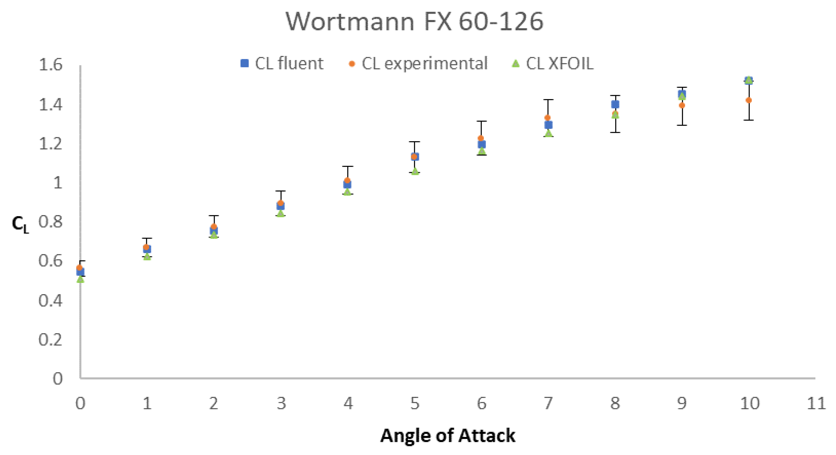
In order to establish the turbulence model for this study and to validate the discretization of fluid domain, a case study was conducted to replicate conditions proposed by Wortmann [43] in his research presented in 1963. The Spalart–Allmaras turbulence model was applied to the aforementioned fluid domain as established in Figure 5, containing the FX 60–126 airfoil with Re = 700,000. Comparison of results with corresponding error bars are shown in Figure 5. Validation is bound within 7% maximum uncertainty.

3.3. Boundary Conditions

These conditions were obtained from average indicated airspeeds at sea level for a set of UAVs shown in Table 1. Boundary conditions observed in Table 3 were applied to both baseline and optimized airfoils. Numerical model used a pressure-based solver with Dirichlet type boundary conditions that had velocity inlet and pressure outlet.

3.4. Convergence Criteria for CFD

Residuals were used as a numerical parameter for convergence. Common residuals established as default by ANSYS-FLUENT were 10−3 for all equations except for energy equation for which it was 10−6 [44]. Considering these parameters as reference, residuals were established as follows: 10−4 for continuity and 10−6 for energy equation. Additionally, monitors were established for the moment, lift, and drag coefficients.

4. Results

This section shows the results of airfoil parameterization, genetic algorithm optimization, and CFD simulations.

4.1. Parameterization

Results of IGP parameterization of the three baseline airfoils are shown in Table 4.
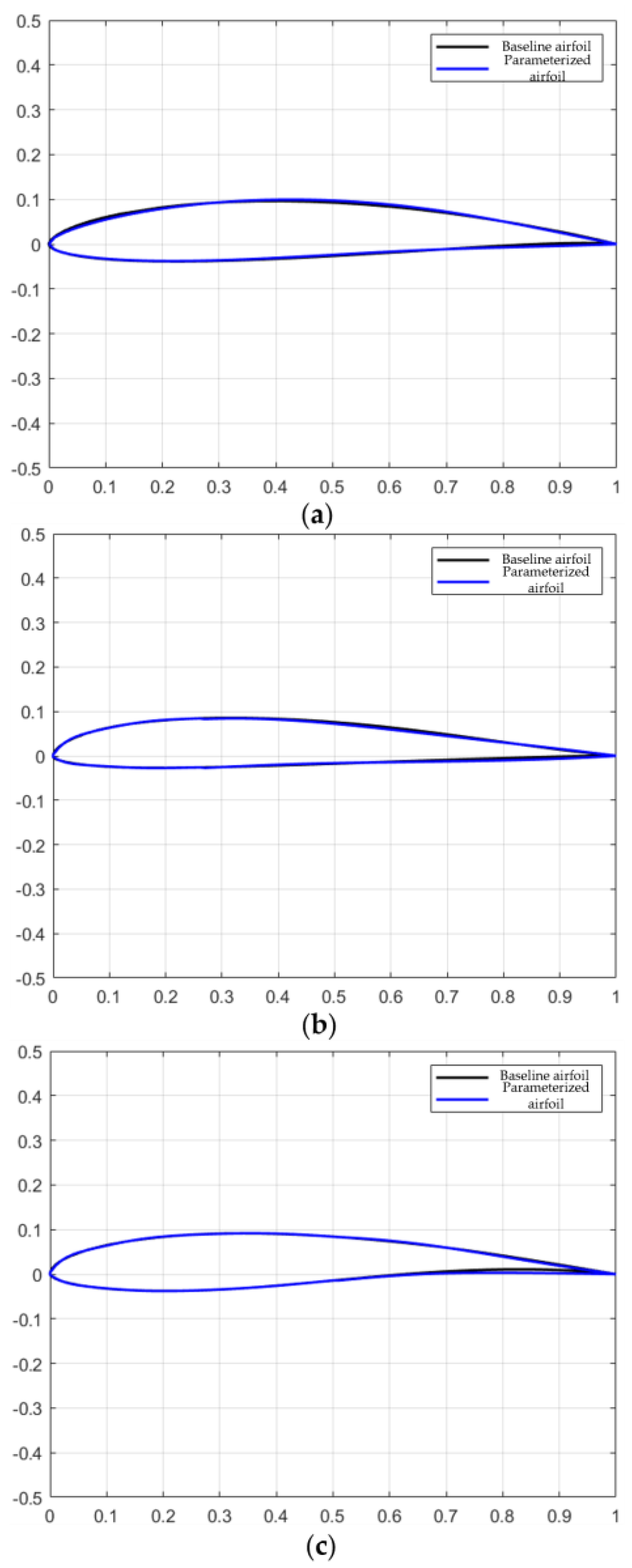
Figure 6 shows the comparison of the baseline airfoils constructed using database x-y coordinates and the baseline airfoils constructed using parameterization. Superposition of airfoils plotted with database coordinates and parameters obtained denotes the level of accuracy of the IGP method. Any minor discrepancy in initial parameterization could be considered as a part of the optimization process given that baseline parameterized airfoils are used as the starting point for optimization to later obtain optimized airfoils; furthermore, CFD numerical models are based on parameterized airfoils for both baseline and optimized cases as illustrated in Section 4.4.2.

4.2. Results of the Genetic Algorithm

Results for the genetic algorithm runs are shown below for the three optimized airfoils under study. Table 5 shows the average of the best adapted CL through the range of angles of attack established for each generation. It is observed that evaluation of fitness function for the best adapted individual from current population is the same as for the previous one; however, convergence is observed in all cases with average CL values higher than the baseline airfoils. Given that this is a stochastic method, each airfoil converges in a different number of iterations.
IGP parameters obtained for the three optimized airfoils are shown in Table 6.
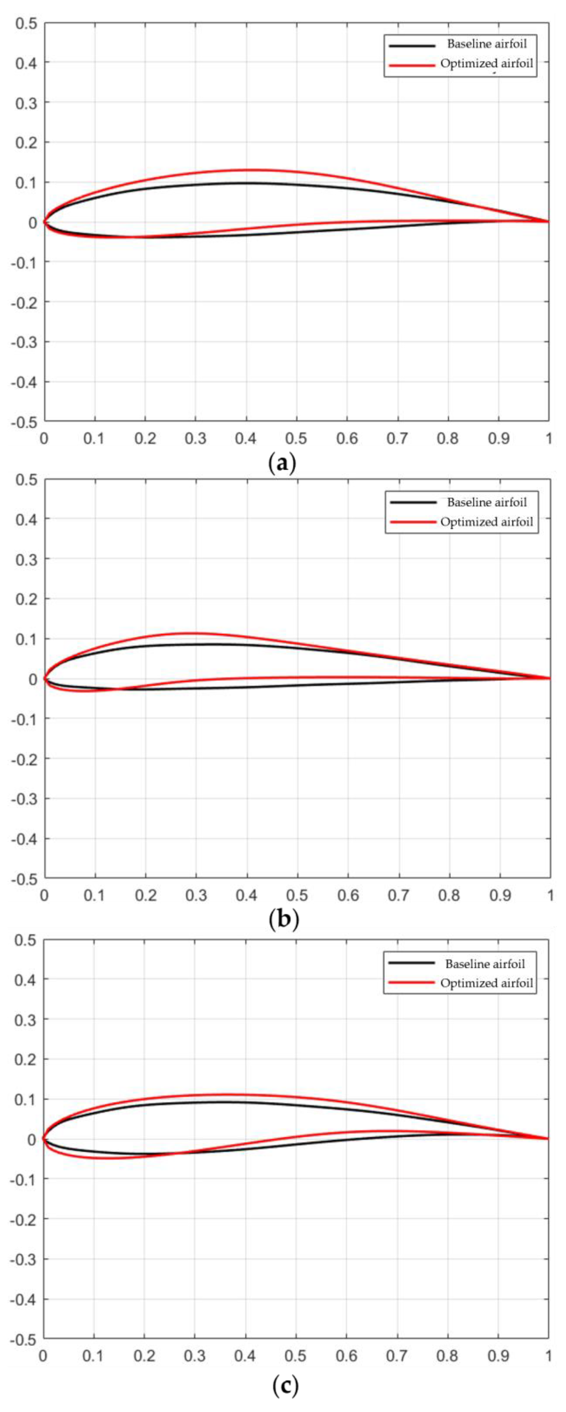
Figure 7 shows a comparison of the baseline and optimized airfoils drawn using IGP parameterization. It is observed that through optimization process, airfoils were reshaped to obtain a higher average CL compared to its original value.

4.3. CFD Simulation Results

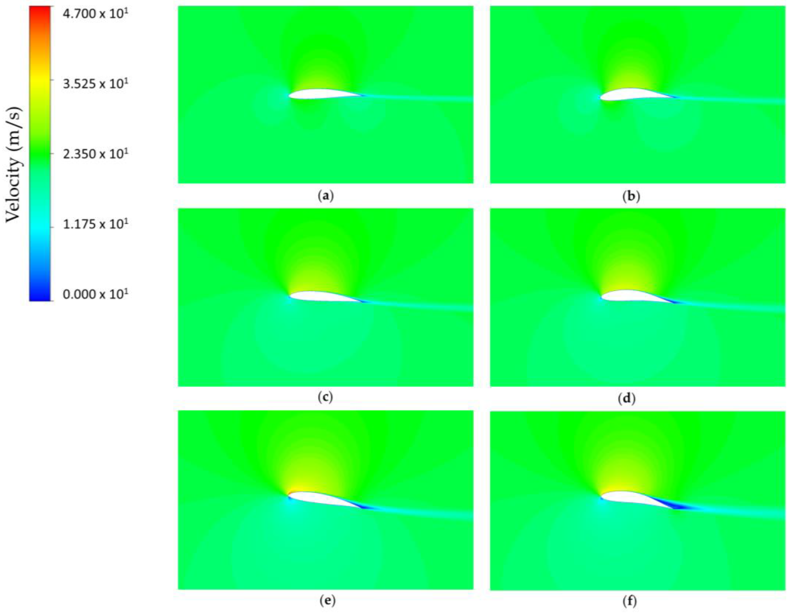
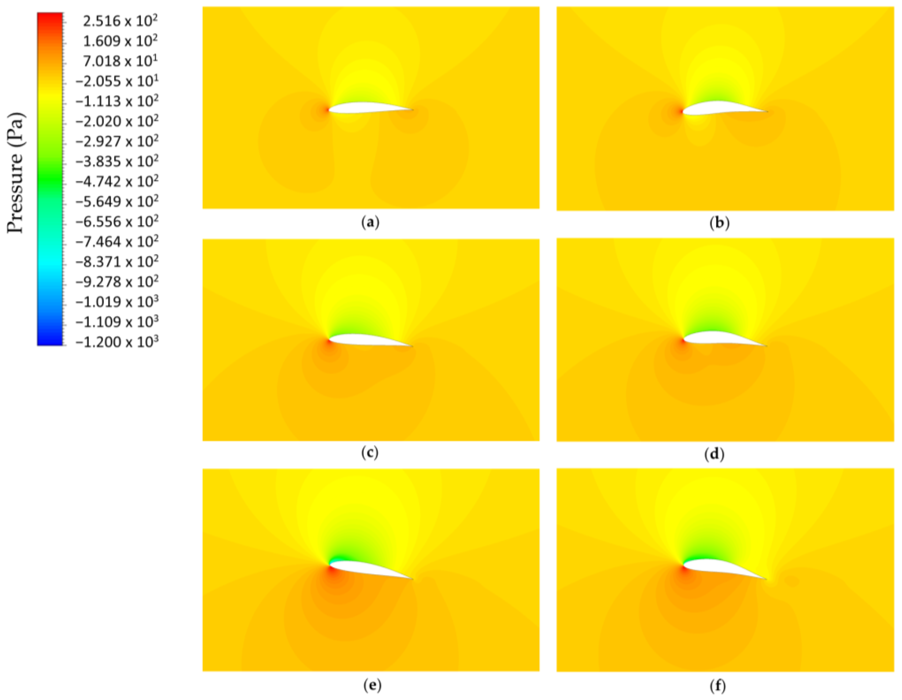
A set of sixty-six simulations were performed, corresponding to the six airfoils analyzed at angles ranging from 0° to 10°. Results presented in this section correspond to the baseline and optimized Eppler 68 airfoil; however, in the next section, all airfoils are analyzed. For showing CFD results, three angles of attack were selected, with 0, 5, and 10 being the minimum, central, and maximum angles.

4.3.1. Velocity Vectors

Figure 8 shows the velocity distribution contours for the Eppler 68 airfoil with the plots (a), (c), and (e) corresponding to baseline airfoil and (b), (d), and (f) corresponding to the optimized one. Comparing velocity contours, it is observed that the maximum speed obtained was 47 m/s. For the case of 0°, it is observed that the velocity distribution varies, obtaining a higher velocity above the extrados of (b) compared to (a). For the 5° case, it is observed that as for 0°, a greater region of high velocities is achieved in the extrados with flow separation occurring at approximately the same chord length for both baseline and optimized airfoils. Finally, for the case of 10°, it is observed that both baseline and optimized airfoils have similar velocity contours; however, separation is more evident in the optimized one. In general, CFD shows that optimized airfoils develop higher velocities compared to baseline airfoils for the three cases, mainly above the extrados.

4.3.2. Pressure Contours

Figure 9 shows pressure contours for the Eppler 68 airfoil ranging from −1200 Pa to 251.6 Pa since they were the minimum and maximum pressures registered in CFD runs. For 0°, 5°, and 10°, improvements regarding pressure distributions are observed. Larger regions of low pressure are present at the extrados of the optimized airfoil; similarly, larger regions of higher pressure are developed at the intrados when compared to the baseline airfoil. This increment in pressure difference for all angles results in a higher CL.

4.4. Optimization Plots

As genetic algorithm runs XFOIL in order to perform aerodynamic analysis during optimization process, the evaluation of fitness function is based on these results; then, CFD is used to analyze results obtained from XFOIL for both baseline and optimized airfoils. Uncertainty between data obtained from XFOIL and CFD is illustrated at the end of this section according to [45].

4.4.1. XFOIL Results

Figure 10 compares baseline and optimized airfoils with the data obtained from XFOIL. Plots show angle of attack vs. CL for (a) Eppler 68, (b) MH 70, and (c) Wortmann FX 60-126. In the three cases, higher CL values are observed for the optimized airfoil as this software was the primary source to evaluate fitness function. In case (b), it is observed that CL increased with an offset mostly constant for all angles of attack. Meanwhile for (a) and (c), a higher improvement in CL is observed at 0 degrees, and it decreases till its minimum at 10 degrees; it is observed that optimized airfoils always show a higher CL as this is the convergence criteria for the genetic algorithm.
Table 7 shows the statistics of improvements from XFOIL data such as average percentage increase in CL and minimum, and maximum increases in CL. From these data, the highest average percentage increase in CL and the maximum CL increase are obtained with the Eppler 68 airfoil. Increments are observed in all cases as these are the criteria that must be met during the optimization process.

4.4.2. CFD Results

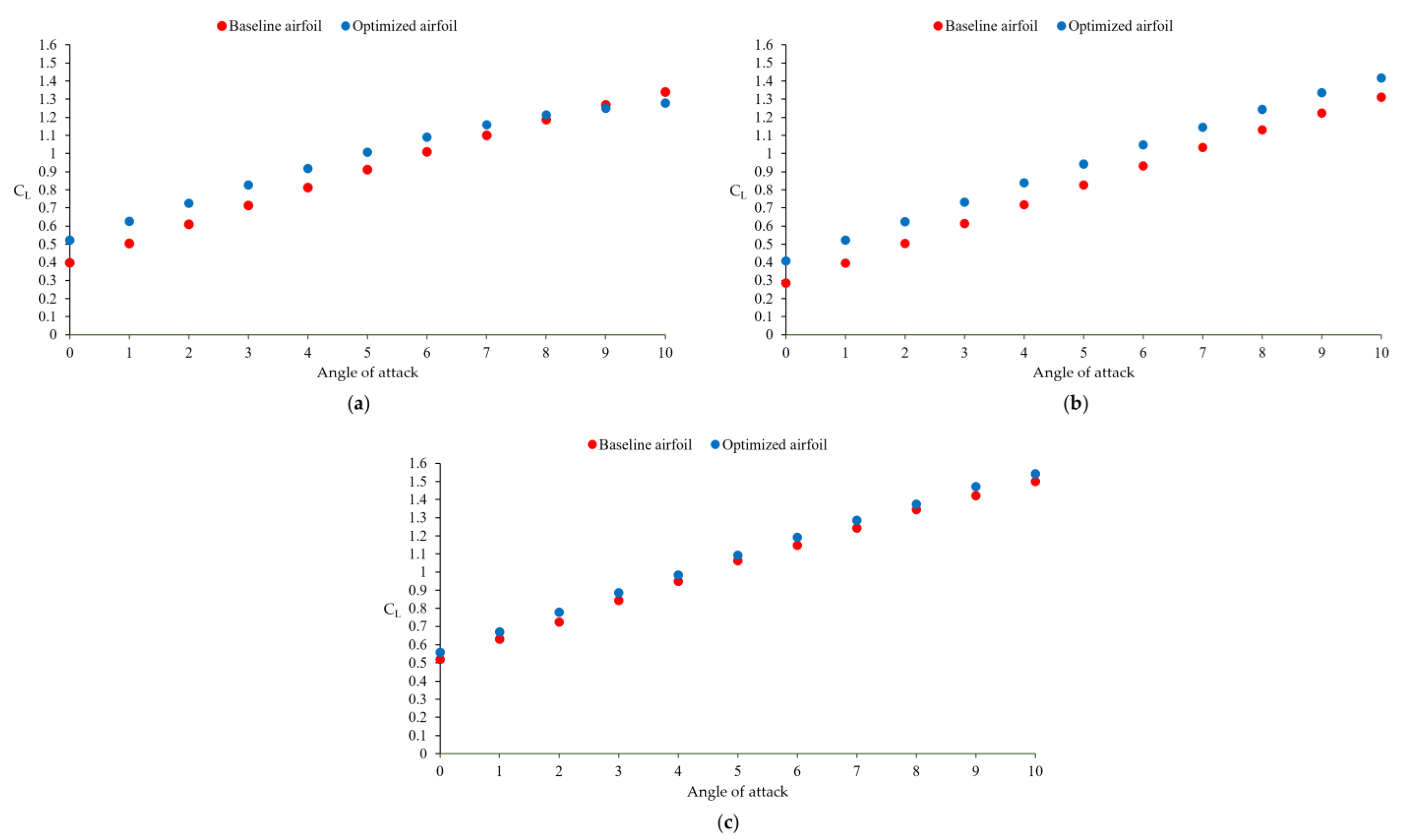
Figure 11 depicts a comparison between baseline and optimized airfoils by analyzing CL vs. angle of attack with data obtained from CFD for (a) Eppler 68, (b) MH 70, and (c) Wortmann FX 60-126. The Eppler 68 airfoil shows a similar trend as observed with XFOIL; it is also observed that at 9° and 10°, CL becomes lower than the baseline airfoil mainly due to viscous effects and separation occurring sooner in the proximity of those angles; however, it is expected that a well-tuned UAV angle of attack does not exceed 5°. The MH 70 airfoil demonstrates the best case of study with an evident increase in CL though the entire range of angles of attack. The Wortmann FX 60-126 airfoil indicates a slight improvement in performance comparing baseline and optimized airfoils.
Table 8 contains further analysis obtained from CFD runs for baseline and optimized airfoils. The highest average percentage increase in CL and the maximum CL increase are obtained with the MH 70 airfoil. It is observed that CL increases mainly for the Eppler 68 and MH 70 airfoils, having a good correlation with the optimization process.

4.4.3. Uncertainty between CFD and XFOIL

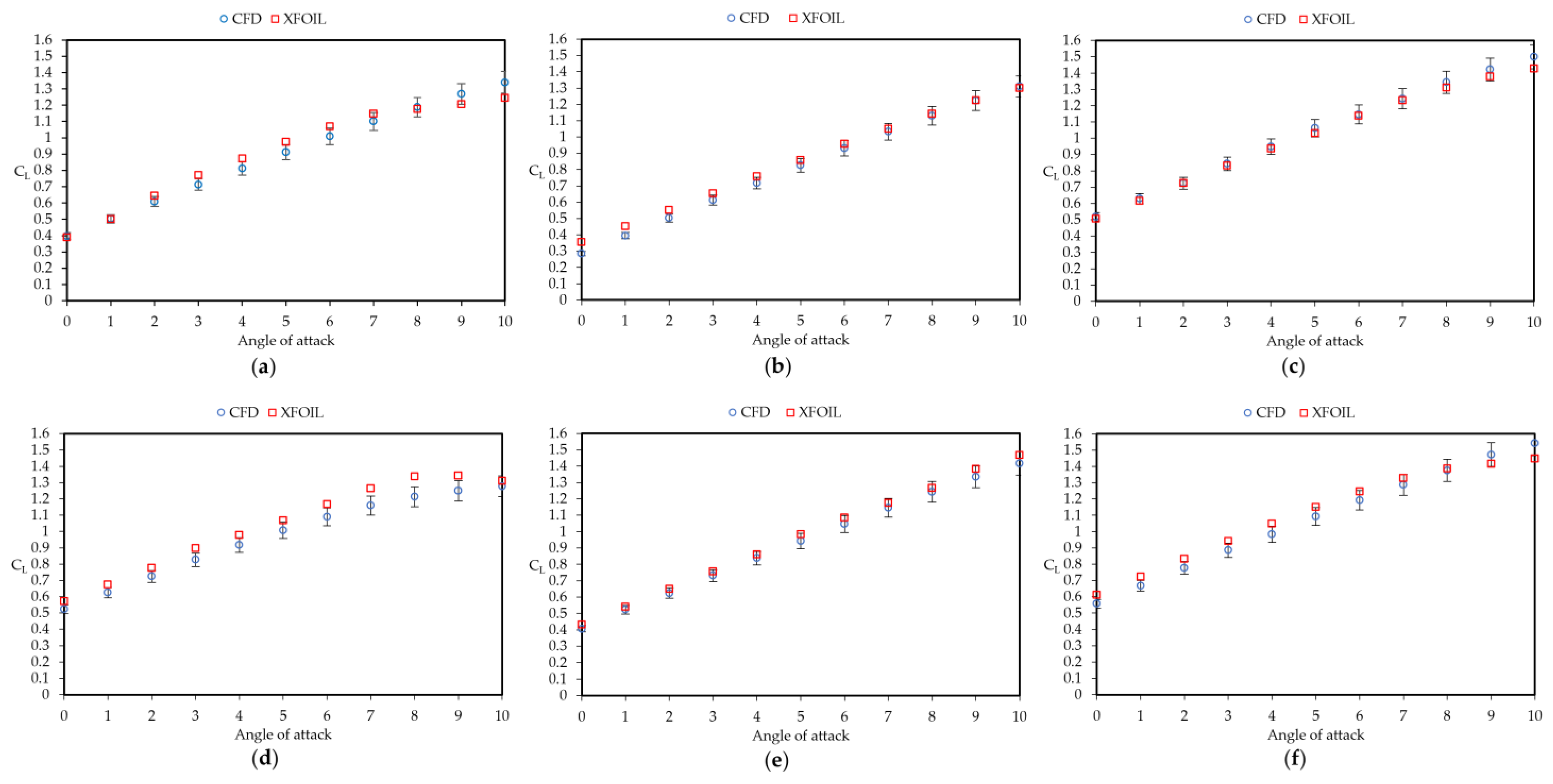
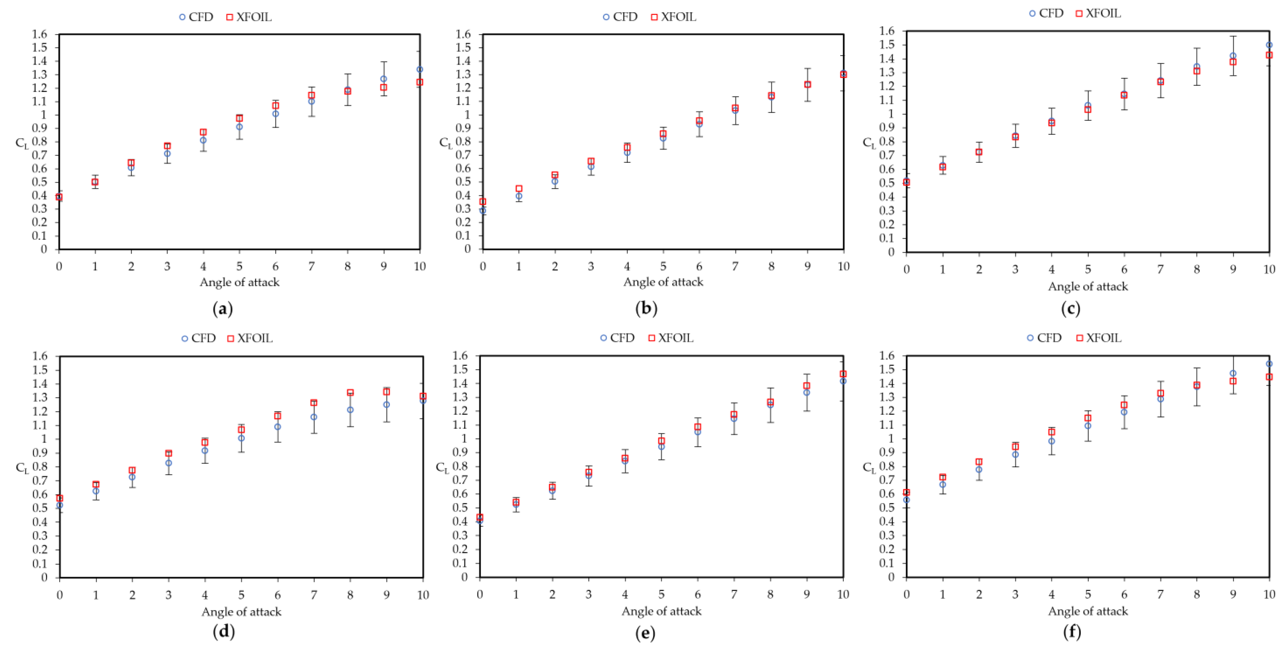
Figure 12 and Figure 13 show a comparison between data obtained from XFOIL and CFD for baseline and optimized airfoils. Figure 12 contains data with 5% uncertainty values centered at the CFD values, and Figure 13 depicts same data with 10% uncertainty. It is observed that for the baseline airfoils predominant uncertainty lies within 5%. A similar behavior is observed for the optimized MH 70 airfoil. For the optimized Eppler 68 and Wortmann FX 60-126 airfoils, uncertainty of data lies mainly within 10% uncertainty.

5. Conclusions

The present study focused on developing a genetic algorithm using the IGP parameterization method, with the objective of optimizing the geometry of three baseline airfoils to increase the lift coefficient and focusing on speeds useful for some unmanned aerial vehicles. The optimized airfoils presented an increase in the average CL of 17.243% for the Eppler 68, 14.967% for the MH 70, and 10.708% for the Wortmann FX 60-126, with respect to their original counterparts with data obtained from XFOIL. For the three baseline and the three optimized airfoils, an average 5.027% uncertainty was obtained in the calculation of the lift coefficient comparing data from XFOIL and CFD.
The research conducted is applicable in the early design phase of an aircraft because it takes parameters from a desired flight envelope as a design starting point. Being a method that modifies the geometry by optimizing a baseline airfoil to increase lift, it must be considered that any shape change will also impact drag. While the optimized airfoils will produce more lift than baseline airfoils, it is necessary to consider that there could be a tradeoff in order to reduce cruise speed due to the increase in lift. Future work is considered to develop more advanced genetic algorithms to optimize aerodynamic efficiency and include it in the fitness function.
The feasibility of parameterizing airfoils by the means of the IGP method and using genetic algorithms for improving aerodynamic characteristics was shown, which could potentially be used for tailoring airfoils for UAVs with specific missions and use them during the design process.
Volume 2 of this study will perform experimental runs in wind tunnel to compare results from XFOIL and CFD.

Author Contributions

Conceptualization, M.E.T.-d.-C. and M.T.-V.; methodology, M.E.T.-d.-C., M.O.V.-Z. and M.T.-V.; software, M.E.T.-d.-C., M.A.F.-A. and M.T.-V.; validation, M.E.T.-d.-C., M.O.V.-Z., M.A.F.-A. and M.T.-V.; formal analysis, M.E.T.-d.-C., M.O.V.-Z. and M.T.-V.; investigation, M.E.T.-d.-C. and M.A.F.-A.; resources, M.O.V.-Z. and J.H.-H.; data curation, M.A.F.-A. and L.d.C.S.-C.; writing—original draft preparation, M.E.T.-d.-C. and M.A.F.-A.; writing—review and editing, M.O.V.-Z. and J.H.-H.; supervision, M.E.T.-d.-C. and M.O.V.-Z.; project administration, L.d.C.S.-C. All authors have read and agreed to the published version of the manuscript.

Funding

This research received no external funding.

Data Availability Statement

Data are contained within the article.

Acknowledgments

M.A.F.-A. thanks Consejo Nacional de Humanidades, Ciencias y Tecnologías, for the scholarship received during his master’s studies.

Conflicts of Interest

The authors declare no conflict of interest. The funders had no role in the design of the study; in the collection, analyses, or interpretation of data; in the writing of the manuscript; or in the decision to publish the results.

References

  1. Raymer, D. Aircraft Design: A Conceptual Approach, 6th ed.; AIAA Education: Reston, VA, USA, 2018; ISBN 978-1-62410-490-9. [Google Scholar]
  2. Selig, M. Low Reynolds Number Airfoil Design Lecture Notes. VKI Lect. Ser. 2003, 2003, 2. [Google Scholar]
  3. Ribeiro, A.F.P.; Awruch, A.M.; Gomes, H.M. An Airfoil Optimization Technique for Wind Turbines. Appl. Math. Model. 2012, 36, 4898–4907. [Google Scholar] [CrossRef]
  4. Katoch, S.; Chauhan, S.S.; Kumar, V. A Review on Genetic Algorithm: Past, Present, and Future. Multimed. Tools Appl. 2021, 80, 8091–8126. [Google Scholar] [CrossRef] [PubMed]
  5. Ray, T.; Tsai, H.M. Swarm Algorithm for Single- and Multiobjective Airfoil Design Optimization. AIAA J. 2004, 42, 366–373. [Google Scholar] [CrossRef]
  6. Khurana, M.; Massey, K. Swarm Algorithm with Adaptive Mutation for Airfoil Aerodynamic Design. Swarm Evol. Comput. 2015, 20, 1–13. [Google Scholar] [CrossRef]
  7. Wickramasinghe, U.K.; Carrese, R.; Li, X. Designing Airfoils Using a Reference Point Based Evolutionary Many-Objective Particle Swarm Optimization Algorithm. In Proceedings of the IEEE Congress on Evolutionary Computation, Barcelona, Spain, 18–23 July 2010; pp. 1–8. [Google Scholar]
  8. Sastry, K.; Goldberg, D.; Kendall, G. Genetic Algorithms. In Search Methodologies: Introductory Tutorials in Optimization and Decision Support Techniques; Burke, E.K., Kendall, G., Eds.; Springer US: Boston, MA, USA, 2005; pp. 97–125. ISBN 978-0-387-28356-2. [Google Scholar]
  9. Ebrahimi, M.; Jahangirian, A. Aerodynamic Optimization of Airfoils Using Adaptive Parameterization and Genetic Algorithm. J. Optim. Theory Appl. 2014, 162, 257–271. [Google Scholar] [CrossRef]
  10. Mukesh, R.; Lingadurai, K.; Selvakumar, U. Airfoil Shape Optimization Using Non-Traditional Optimization Technique and Its Validation. J. King Saud Univ.-Eng. Sci. 2014, 26, 191–197. [Google Scholar] [CrossRef]
  11. Della Vecchia, P.; Daniele, E.; D’Amato, E. An Airfoil Shape Optimization Technique Coupling PARSEC Parameterization and Evolutionary Algorithm. Aerosp. Sci. Technol. 2014, 32, 103–110. [Google Scholar] [CrossRef]
  12. Lee, D.S.; Gonzalez, L.F.; Srinivas, K.; Periaux, J. Robust Evolutionary Algorithms for UAV/UCAV Aerodynamic and RCS Design Optimisation. Comput. Fluids 2008, 37, 547–564. [Google Scholar] [CrossRef]
  13. Pons-Prats, J.; Bugeda, G.; Zárate, F.; Oñate, E. Optimización Robusta En Aplicaciones Aeronáuticas Con La Combinación de Cálculo Estocástico y Algoritmos Evolutivos. Rev. Int. De Métodos Numéricos Para Cálculo Y Diseño En Ing. 2012, 28, 18–32. [Google Scholar] [CrossRef]
  14. Ram, K.R.; Lal, S.; Rafiuddin Ahmed, M. Low Reynolds Number Airfoil Optimization for Wind Turbine Applications Using Genetic Algorithm. J. Renew. Sustain. Energy 2013, 5, 052007. [Google Scholar] [CrossRef]
  15. Shinde, P.; Ohol, S.S.; Tripathi, V.K. Production Design Analysis for Airfoil Shape Optimization; Social Science Research Network: Rochester, NY, USA, 2021. [Google Scholar]
  16. Chen, J.; Yang, H.; Yang, M.; Xu, H.; Hu, Z. A Comprehensive Review of the Theoretical Approaches for the Airfoil Design of Lift-Type Vertical Axis Wind Turbine. Renew. Sustain. Energy Rev. 2015, 51, 1709–1720. [Google Scholar] [CrossRef]
  17. Masters, D.A.; Taylor, N.J.; Rendall, T.C.S.; Allen, C.B.; Poole, D.J. Geometric Comparison of Aerofoil Shape Parameterization Methods. AIAA J. 2017, 55, 1575–1589. [Google Scholar] [CrossRef]
  18. Jiang, H.B.; Li, Y.R.; Cheng, Z.Q. Methods of Constructing Analytic Functions to Generate Airfoil Profiles; Atlantis Press: Paris, France, 2015; pp. 221–223. [Google Scholar]
  19. Ziemkiewicz, D. Simple Parametric Model for Airfoil Shape Description. AIAA J. 2017, 55, 4390–4393. [Google Scholar] [CrossRef]
  20. Lu, X.; Huang, J.; Song, L.; Li, J. An Improved Geometric Parameter Airfoil Parameterization Method. Aerosp. Sci. Technol. 2018, 78, 241–247. [Google Scholar] [CrossRef]
  21. Sripawadkul, V.; Padulo, M.; Guenov, M. A Comparison of Airfoil Shape Parameterization Techniques for Early Design Optimization; American Institute of Aeronautics and Astronautics: Fort Worth, TX, USA, 2010. [Google Scholar]
  22. Dahl, K.S.; Fuglsang, P. Design of the Wind Turbine Airfoil Family RISOe-A-XX; Risoe National Laboratory, Wind Energy and Atmospheric Physics Department: Roskilde, Denmark, 1998. [Google Scholar]
  23. Fuglsang, P.; Bak, C.; Gaunaa, M.; Antoniou, I. Design and Verification of the Risø-B1 Airfoil Family for Wind Turbines. J. Sol. Energy Eng. 2004, 126, 1002–1010. [Google Scholar] [CrossRef]
  24. Méndez, B.; Munduate, X.; Miguel, U.S. Airfoil Family Design for Large Offshore Wind Turbine Blades. J. Phys. Conf. Ser. 2014, 524, 012022. [Google Scholar] [CrossRef]
  25. Miller, M.; Lee Slew, K.; Matida, E. The Development of a Flatback Wind Turbine Airfoil Family. Wind. Energy 2018, 21, 1372–1382. [Google Scholar] [CrossRef]
  26. Doosttalab, M.; Frommann, O. Multidisciplinary Design and Verification of the HB Flatback Airfoil Family. AIAA J. 2019, 57, 4639–4649. [Google Scholar] [CrossRef]
  27. Nex, F.; Armenakis, C.; Cramer, M.; Cucci, D.A.; Gerke, M.; Honkavaara, E.; Kukko, A.; Persello, C.; Skaloud, J. UAV in the Advent of the Twenties: Where We Stand and What Is Next. ISPRS J. Photogramm. Remote Sens. 2022, 184, 215–242. [Google Scholar] [CrossRef]
  28. Günel, O.; Koç, E.; Yavuz, T. CFD vs. XFOIL of Airfoil Analysis at Low Reynolds Numbers. In Proceedings of the 2016 IEEE International Conference on Renewable Energy Research and Applications (ICRERA), Birmingham, UK, 20–23 November 2016; pp. 628–632. [Google Scholar]
  29. Mokhtar, W. A Numerical Parametric Study of High-Lift Low Reynolds Number Airfoils. In 43rd AIAA Aerospace Sciences Meeting and Exhibit; Aerospace Sciences Meetings; American Institute of Aeronautics and Astronautics: Reston, VA, USA, 2005. [Google Scholar]
  30. Traub, L.W.; Coffman, C. Efficient Low-Reynolds-Number Airfoils. J. Aircr. 2019, 56, 1987–2003. [Google Scholar] [CrossRef]
  31. Morgado, J.; Vizinho, R.; Silvestre, M.A.R.; Páscoa, J.C. XFOIL vs CFD Performance Predictions for High Lift Low Reynolds Number Airfoils. Aerosp. Sci. Technol. 2016, 52, 207–214. [Google Scholar] [CrossRef]
  32. Srinivas, G.; Gowda, B.P. Aerodynamic Performance Comparison of Airfoils by Varying Angle of Attack Using Fluent and Gambit. Appl. Mech. Mater. 2014, 592–594, 1889–1896. [Google Scholar] [CrossRef]
  33. Airfoil Tools. Available online: http://www.airfoiltools.com/ (accessed on 17 December 2023).
  34. Rincón, J.C. Aplicación De Algoritmos Genéticos En La Optimización Del Sistema De Abastecimiento De Agua De Barquisimeto-Cabudare. Av. En Recur. Hidráulicos 2006, 14, 25–38. [Google Scholar]
  35. Lavinas, Y.; Aranha, C.; Sakurai, T.; Ladeira, M. Experimental Analysis of the Tournament Size on Genetic Algorithms. In Proceedings of the 2018 IEEE International Conference on Systems, Man, and Cybernetics (SMC), Miyazaki, Japan, 7–10 October 2018; pp. 3647–3653. [Google Scholar] [CrossRef]
  36. Fang, Y.; Li, J. A Review of Tournament Selection in Genetic Programming. In Proceedings of the Advances in Computation and Intelligence, Wuhan, China, 22–24 October 2010; Cai, Z., Hu, C., Kang, Z., Liu, Y., Eds.; Springer: Berlin/Heidelberg, Germany, 2010; pp. 181–192. [Google Scholar]
  37. Patil, B.S.; Thakare, H.R. Computational Fluid Dynamics Analysis of Wind Turbine Blade at Various Angles of Attack and Different Reynolds Number. Procedia Eng. 2015, 127, 1363–1369. [Google Scholar] [CrossRef]
  38. Prisacariu, V. CFD Analysis of UAV Flying Wing. Incas Bull. 2016, 8, 65–72. [Google Scholar] [CrossRef]
  39. Versteeg, H.K.; Malalasekera, W. An Introduction to Computational Fluid Dynamics: The Finite Volume Method, 2nd ed.; Pearson Education Ltd.: Harlow, UK, 2007; Pearson Education Ltd.: New York, NY, USA, 2007; ISBN 978-0-13-127498-3. [Google Scholar]
  40. Winnemöller, T.; Van Dam, C.P. Design and Numerical Optimization of Thick Airfoils Including Blunt Trailing Edges. J. Aircr. 2007, 44, 232–240. [Google Scholar] [CrossRef]
  41. Xu, X.; Zhou, Z.; Fan, R.; Wang, J. Investigation of Active Flow Control on Aerodynamic Performance of HALE UAV Airfoil. In Proceedings of the 2010 Second International Conference on Computer Modeling and Simulation, Sanya, China, 22–24 January 2010; Volume 4, pp. 123–126. [Google Scholar]
  42. Bagul, P.; Rana, Z.A.; Jenkins, K.W.; Könözsy, L. Computational Engineering Analysis of External Geometrical Modifications on MQ-1 Unmanned Combat Aerial Vehicle. Chin. J. Aeronaut. 2020, 33, 1154–1165. [Google Scholar] [CrossRef]
  43. Wortmann, F.X. Einige Laminarprofile für Segelflugzeuge; 9 OSTIV-Kongress: Junin, Argentinien, 1963. [Google Scholar]
  44. ANSYS Fluent User’s Guide; ANSYS: Canonsburg, PA, USA, 2016.
  45. Maupin, K.A.; Swiler, L.P.; Porter, N.W. Validation Metrics for Deterministic and Probabilistic Data. J. Verif. Valid. Uncertain. Quantif. 2019, 3, 031002-1–031002-10. [Google Scholar] [CrossRef]
Figure 1. Design process flowchart.
Aerospace 11 00044 g001
Figure 2. IGP geometric parameters.
Aerospace 11 00044 g002
Figure 3. Flowchart of the developed genetic algorithm.
Aerospace 11 00044 g003
Figure 4. (a) Entire mesh, (b) mesh around airfoil, and (c) mesh at the boundary layer.
Aerospace 11 00044 g004
Figure 5. Wortmann experimental data comparison at Re = 700,000.
Aerospace 11 00044 g005
Figure 6. Comparison of baseline airfoils drawn with x-y coordinates and parameterization: (a) Eppler 68, (b) MH 70, and (c) Wortmann FX 60-126.
Aerospace 11 00044 g006
Figure 7. Comparison of parameterized baseline and optimized airfoils: (a) Eppler 68, (b) MH 70, and (c) Wortmann FX 60-126.
Aerospace 11 00044 g007
Figure 8. Comparison of velocity profiles for baseline Eppler 68 at angles, (a) 0°, (c) 5°, and (e) 10°, with respect to optimized Eppler 68 at angles, (b) 0°, (d) 5°, and (f) 10°.
Aerospace 11 00044 g008
Figure 9. Comparison of pressure contours for baseline Eppler 68 at angles, (a) 0°, (c) 5°, and (e) 10°, with respect to optimized Eppler 68 at angles, (b) 0°, (d) 5°, and (f) 10°.
Aerospace 11 00044 g009
Figure 10. Comparison of CL vs. angle of attack for baseline and optimized airfoils: (a) Eppler 68, (b) MH 70, and (c) Wortmann FX 60-126, with data obtained from XFOIL.
Aerospace 11 00044 g010
Figure 11. Comparison of CL vs. angle of attack for baseline and optimized airfoils: (a) Eppler 68, (b) MH 70, and (c) Wortmann FX 60-126, with data obtained from CFD.
Aerospace 11 00044 g011
Figure 12. 5% uncertainty plot between data from CFD and XFOIL for baseline airfoils, (a) Eppler 68, (b) MH 70, and (c) Wortmann FX 60-126, and optimized airfoils, (d) Eppler 68, (e) MH 70, and (f) Wortmann FX 60-126.
Aerospace 11 00044 g012
Figure 13. 10% uncertainty plot between data from CFD and XFOIL for baseline airfoils, (a) Eppler 68, (b) MH 70, and (c) Wortmann FX 60-126, and optimized airfoils, (d) Eppler 68, (e) MH 70, and (f) Wortmann FX 60-126.
Aerospace 11 00044 g013
Table 1. Reynolds and Mach numbers for selected UAVs.
ParameterReynolds NumberMach Number
UAV 1 101,5200.0275
UAV 2276,8220.0868
UAV 3271,6630.0686
UAV 4356,4490.0878
UAV 5363,2190.0607
UAV 6323,0120.0894
UAV 7574,3510.0805
UAV 8642,9890.1133
Table 2. Features of three meshes for mesh sensitivity analysis.
ParameterMesh 1Mesh 2Mesh 3
Number of elements200,900128,72072,540
Number of nodes200,000128,00072,000
Face size666
Edge sizing number181818
Maximum ortho skew0.4850.4870.491
Minimum orthogonal quality0.5140.5120.508
Table 3. Boundary conditions.
PropertyValue
Velocity22 m/s
Viscosity1.789 × 10−5 kg/ms
Density1.225 kg/m3
Temperature288.15 k
Molecular weight28.97 mol
Specific heat1.007 KJ/kg K
Thermal conductivity0.0253 W/m K
Table 4. Parameterization of the baseline airfoils.
Airfoil C X C T X T b X c ρ 0 α T E β T E
Eppler 68 0.03334210.51839470.13106990.35451510.21834930.24305160.10416071.4664183
MH 700.03087080.38127090.10994430.26421410.25742860.23838150.04118691.6385809
Wortmann FX 60-1260.03558570.57525080.12531410.26755850.26724250.26486040.10094380.8993897
Table 5. Winning average CL for airfoils Eppler 68, MH 70, and Wortmann FX 60-126 by generation.
Eppler 68 MH 70Wortmann FX 60-126
Number of GenerationsWinning Average CL Number of GenerationsWinning Average CL Number of GenerationsWinning Average CL Number of GenerationsWinning Average CL
10.84867273141.0140454510.8666090911.03812727
20.87700909151.0140454520.8666090921.03812727
30.87700909161.0352545530.8666090931.03812727
40.87700909171.0352545540.8666545541.03866364
50.96570909181.0352545550.8666545551.03866364
60.96570909191.0352545560.8666545561.07715455
70.97150909201.0352545570.8666545571.09464545
81.01368182211.0352545580.9163272781.09464545
91.01368182221.0352545590.9163272791.09464545
101.01368182231.03525455100.91632727101.09464545
111.01368182241.03525455110.96380909111.09464545
121.01368182251.03525455 121.09464545
131.01368182261.03527273 131.10314545
Table 6. Parameterization of the optimized airfoils.
Airfoil C X C T X T b X c ρ 0 α T E β T E
Eppler 68 0.037456130.470359120.151319850.31560550.233651060.329063810.148068680.93750603
MH 700.03502600.333613820.122581090.216630740.348689410.255705800.097494091.30056557
Wortmann FX 60-1260.035226930.523294780.144755790.222770390.427393780.269840990.152415690.73403739
Table 7. Statistics of improvements of optimized and baseline airfoils from XFOIL.
AirfoilAverage Percentage Increase in CLMinimum CL IncreaseMaximum CL Increase
Eppler 6817.2430.06820.1814
MH 7014.9670.0770.1689
Wortmann FX 60-12610.7080.02150.1188
Table 8. Statistics of improvements of optimized and baseline airfoils from CFD.
AirfoilAverage Percentage Increase in CLMinimum CL IncreaseMaximum CL Increase
Eppler 6812.3280.06150.1252
MH 7018.1710.10650.1284
Wortmann FX 60-1264.4440.03110.0532
Disclaimer/Publisher’s Note: The statements, opinions and data contained in all publications are solely those of the individual author(s) and contributor(s) and not of MDPI and/or the editor(s). MDPI and/or the editor(s) disclaim responsibility for any injury to people or property resulting from any ideas, methods, instructions or products referred to in the content.