An Unsteady Reynolds–Averaged Navier–Stokes–Large Eddy Simulation Study of Propeller–Airframe Interaction in Distributed Electric Propulsion

Abstract

A conceptual framework is presented to determine the improvement in the aerodynamic performance of a canard aircraft fitted with distributed propellers along its main wing. A preliminary study is described with four airframe–propeller configurations predominantly studied in academic and commercial designs. The leading edge–based tractors and trailing edge–based pushers are identified as configurations of interest for the main study. Subsequently, a Navier–Stokes solver is used to simulate the flow using two numerical approaches–a modified steady-state actuator disk and an unsteady rotating propeller profile. Moving meshes with rotating sub-domains are used with a hybrid RANS-LES-based turbulence model while the actuator disks are modified to include viscous swirl effects. The preliminary study shows a local minimum in the change in $C_L$ and $C_D$ at 10${}^{\circ }$ for the pusher and tractor configurations. The main study then demonstrates the outperformance of the pushers over tractors quantified using $C_L$ and $C_L/C_D$. There is a clear preference for the pushers as they increase the lifting capacity of the aircraft without disproportionately increasing the drag due to the flow smoothening by the suction of the pusher propellers over the main wing. The pushers also delay the separation of the boundary layer whereas the tractors are unable to prevent the formation of the separation bubble despite injecting momentum through their slipstreams into the flow. The results from the two numerical approaches are then compared for accuracy in designing DEP configurations for an airframe.

1. Introduction

Conventional fuel-based powerplants including internal combustion and gas turbine/jet-based engines have been the go-to propulsion systems for automobiles and aircraft, respectively, but are constrained by their scalability and efficiency. Modern battery technology has enabled the commercial use of electric power systems in automobiles and aircraft in the form of electric and combustion–electric hybrid aircraft. Cheap and affordable transport can be offered to ferry passengers and cargo if a scalable cost-effective electric aircraft propulsion system is developed. The integration of electric powerplants in aircraft designs for use in conjunction with fuel-based powerplants is typically quantified using a degree of hybridization [1,2]. The limitations of conventional designs can be overcome by a promising solution that involves several small-sized electrically powered propellers distributed over the lifting surfaces and the fuselage of the aircraft. Distributed electric propulsion (DEP) has demonstrated improvement in the efficiency of aircraft and lowering of its noise signatures without additional structural changes to the airframe [3].

This concept has been implemented in several academic, industrial, and commercial ventures such as NASA’s LEAPTech X-57 Maxwell, ESAero’s ECO-150, a 150-seater turboelectric aircraft, Lilium, Airbus’ 1-passenger tilt-wing Vahana, Ehang’s autonomous aerial vehicle and its VT-30 variant, Joby aviation’s multi-rotor VTOL aircraft, and Kittyhawk’s remotely piloted 1-seater airtaxi. An overview of the various DEP concepts currently being employed that possess disruptive capabilities for air transport is available in the literature [4]. Projects using enhanced aerodynamic designs enabled by DEP encourage us to look further into optimized DEP configurations for electric aviation solutions [5]. A comparison of different representative designs of aircraft like multi-rotors, fixed-wing–rotor combinations, and vectored thrusters using DEP revealed that a distributed configuration is more efficient in cruise mode and offers better range [6].

A civilian four-seater aircraft modified to retrofit a DEP configuration has demonstrated a high $C_{Lmax}$ and a relatively flat lift curve due to its distributed propeller placement, indicating an increased aircraft efficiency [7]. Another application of DEP is for a two-seater short–haul aircraft with eight leading-edge tilting propellers and four V-tail propellers [8]. The numerical analysis of the X-57 Maxwell showed a high cruise $C_L=0.75$ at zero angle of attack [9,10]. The experimental counterpart to that study retrofitted a DEP configuration in place of an internal combustion engine, revealing a significant reduction in the required wing area with a five-fold drop in energy requirement in cruise mode [11]. Retrofitting DEP onto wings has shown that increasing the number of propellers reduces the takeoff distance by over 50% [12].

Numerical studies using the vortex panel–particle hybrid method have also been used to analyze the influence of propeller slipstream on a wing [13]. A numerical study on the performance of tip-mounted propellers using a one-equation RANS model showed that the use of the actuator disk model for studying the slipstream–wing interaction reduces the computational cost by 85% [14]. High-resolution unsteady analysis of propeller–fixed wing interaction indicates that the actuator disk model agrees well with the mean lift and drag characteristics of the unsteady flow for most spanwise locations [15]. Other studies of UAV–propeller aerodynamic interaction include those on aero–elastic propeller interaction [16], inviscid flow analysis [17], effects of propeller position on pressure over the wing [18,19], large eddy simulation (LES) studies on tip–vortex shedding [20], detached eddy simulation (DES) studies of a propeller wake [21], quasi–steady 3D numerical studies for shrouded propellers [22], and multiple reference frame (MRF) studies for slow flyer propellers [23]. This encourages us to use the actuator disk approach along with a high–fidelity DES approach to estimate the aerodynamic performance of multi–propeller configurations. Experimental studies of distributed propellers in wind tunnels reveal a negative efficiency correlation with angle of attack and highly 3D flows for different numbers of propellers placed in an array [24,25]. Wing-tip–mounted propellers in tractor and pusher configurations in a wind tunnel study found that pushers required the lowest power for a desired lift coefficient while the tractors increased the aerodynamic efficiency of the wing [26]. This motivates us to investigate the tractor and pusher configurations in further detail in the main study of the present paper.

Amidst the variety of DEP designs that are available, there does not seem to be a consensus on the optimal placement of propellers relative to the wing and airframe, which is where the present study aims to contribute. While some designs like Maxwell, ECO–150, Vahana, and Joby use a leading edge–based tractor configuration, some designs like Lilium and Kittyhawk use a trailing edge–based pusher configuration for their propellers/ducted fans. However, there is a lack of comprehensive comparison of the various propeller placements to be used in a DEP configuration. Since the existing literature and the commercially available designs do not comment on the optimal propeller placement subject to constraints of the available aircraft’s design, the present study takes up that task. We first introduce the reader to a preliminary analysis of the prevailing DEP configurations using a steady–state modified actuator disk approach, which is a RANS–based solver, to gain insights and motivation for the main study. The main study is then conducted using an unsteady rotating propeller approach that employs detached eddy simulation (DES) on the tractor and pusher configurations for a detailed flow field analysis based on the insights gained from the preliminary study. The tractor and pusher configurations require special attention due to their blowing versus the suction effect of their propeller slipstreams as well. We then compare the accuracy of the steady–state results with the results from the unsteady solver for the two DEP configurations to quantitatively analyze their aerodynamic characteristics.

The steady–state approach uses a modified actuator disk model to include swirl effects in its slipstream to obtain a realistic recreation of propeller–airframe interaction. The unsteady rotating propeller approach simulates the development of propeller slipstreams using moving meshes. The modified actuator disk approach is based on the $k-\omega$ SST RANS model whereas the rotating propeller approach uses a hybrid implementation of $k-\omega$ SST RANS and LES turbulence modeling, called DES. The DES turbulence modeling is chosen for its ability to accurately capture flow features like the shedding of the tip–vortices from propeller blades and their interaction with the UAV airframe. It is able to capture the characteristic flow features in three–dimensional flows without requiring large mesh counts. Both the numerical approaches are used for the pusher and tractor configurations for $\alpha$ = 8${}^{\circ }$ to 14${}^{\circ }$ operating in a freestream with $U_{\infty }$ = 100 km/h. The present study thus attempts to compare the two contrasting UAV–propeller DEP configurations prevailing in academic and commercial designs by establishing a conceptual framework for the estimation of their aerodynamic performance that can then be applied to the analysis of a general DEP design as well.

2. Materials and Methods

This section describes the geometric setup, meshing, and numerical implementation used in this paper.

2.1. Geometry

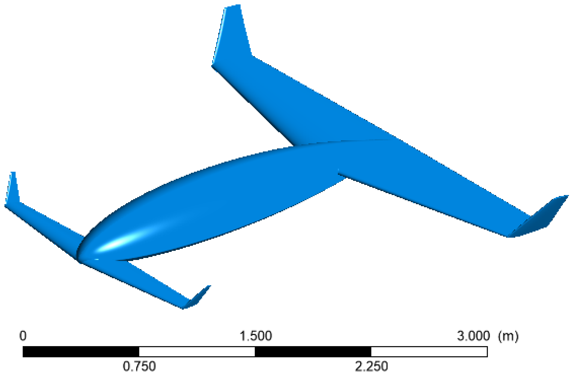
The novel canard aircraft used in this study is a UAV meant to operate a 25–50 kg payload. Its geometric details have been given in

Table 1. Geometric details of the UAV airframe.

Geometric Feature	Value
Airframe length	3 m
Main wing span	2.7 m
Canard wing span	1.62 m
Main wing root chord	0.8 m
Canard wing root chord	0.32 m
Wing taper ratio	2:1
Wetted surface area	7.177 m${}^2$

. Since this study offers a framework to analyze a DEP configuration in general, the choice of this UAV is due to its availability and our intention to experimentally test it in the future in a wind tunnel. Both wings of the UAV, main and canard, are based on a modified NACA0012 airfoil designed to achieve the desired aerodynamic performance. The aerodynamic performance of the airframe has been studied in detail [27,28,29] and is also illustrated in Section 3.4. See Figure 1 for the geometry of the UAV airframe.

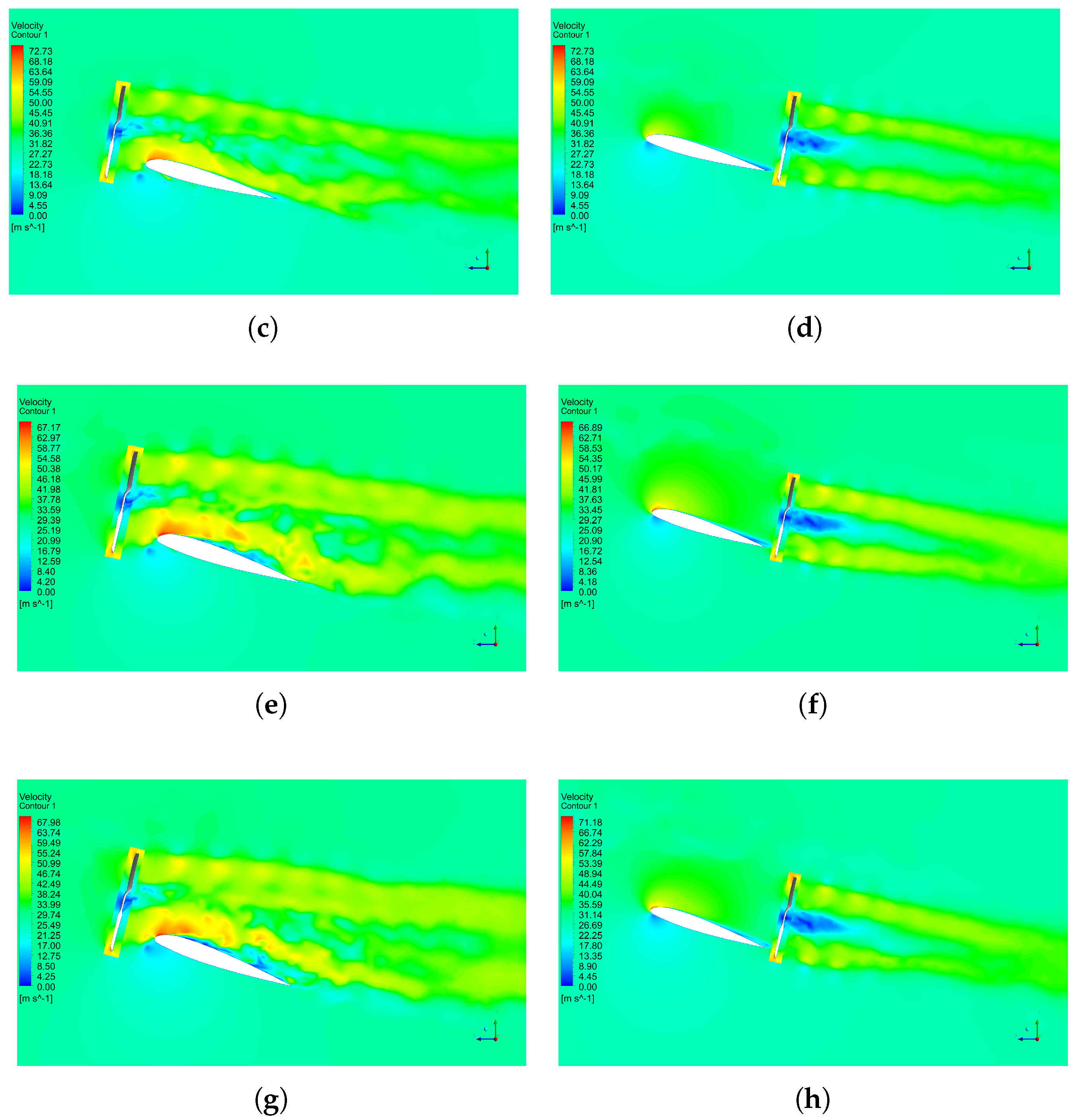
The planform area of the main wing is taken as the reference area for all calculations, and is 1.62 m${}^2$. The UAV airframe will be augmented with four propellers in the main study, placed two per side, to set up the tractor– and pusher–based DEP configurations. The propeller used in this study is a custom–designed two–bladed propeller based on the Clark–Y airfoil designed to yield a high propeller efficiency over a wide range of advance ratios. It has a diameter D = 18 in (=0.4572 m). Its geometric details, namely chord and pitch profiles, are given in Figure 2.

Four propellers are placed along the leading edge (as tractors) and trailing edge (as pushers) of the main wing, studied separately. This is to compare the blowing versus the suction effect of the propellers, respectively. The propeller motion is simulated using two numerical approaches–using modified actuator disks and rotating propeller profiles with moving meshes. The propellers are spaced $1.2D$ from the fuselage axis and each other. The propellers are also vertically offset above the wing plane by a height of $D/4$ to account for the structural constraints in accommodating the motor–propeller units on the wing frame and based on the findings of the preliminary study. For the tractor configuration, the propellers are aligned in parallel with the taper of the main wing. For the pusher configuration, all the propellers are co–planar and placed $0.22D$ behind the trailing edge of the main wing.

To implement the actuator disks, 2D circular disks each of diameter D are created in the propeller planes passing through the respective propeller hubs. To implement the moving meshes for the rotating propeller approach, a sub–domain is created around each propeller which will rotate in the domain to simulate the propeller motion. Each rotating sub–domain is a right circular cylinder of 1.1D diameter and 0.15D height, with the propeller centered in the rotating sub–domain, drawing from the setup used by Kutty et al. [23]. The propellers on the left wing rotate in a counter–clockwise sense as seen from the front of the aircraft and those on the right wing rotate in a clockwise sense to counter the net yaw produced.

This study is performed keeping in mind the authors’ intentions to recreate the configurations in an experimental setup in the future by performing wind tunnel studies of the UAV–propeller configurations. Thus, the outer domain is sized accordingly and is a cuboid of dimensions 4 m × 4.5 m × 10 m. The outlet face of the domain is placed at 6 m from the trailing edge of the aircraft, which is approximately $13D$ distance from the propeller plane for the pusher configuration and $15D$ distance for the tractor configuration, giving the propeller slipstreams enough distance to allow for their full spatial development.

To reduce the computational cost of the setup, all studies are conducted by performing the simulations for the UAV airframe split longitudinally by its plane of symmetry along with two propellers. We shall refer to the propeller closer to the fuselage axis as first and the farther as second hereon.

2.2. Meshing

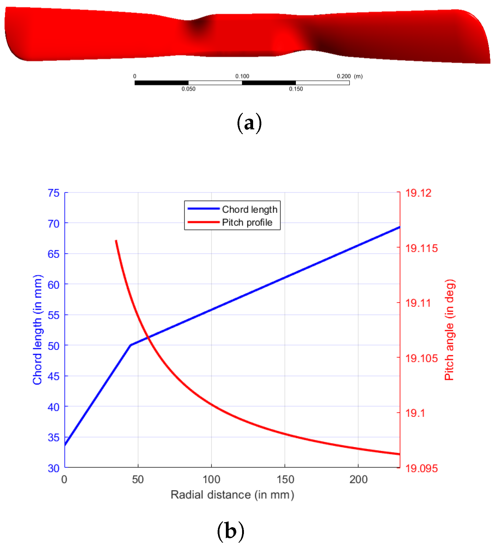
A good quality mesh with a lower cell count is desirable since the flow features need to be captured with sufficient accuracy with minimum possible computational time and cost. A non–conformal tetrahedral mesh is generated for the domain and rotating sub–domains of propellers. A non–dimensionalized first–cell height is maintained $y^{+}$ < 5 for the walls of the airframe and propeller blades using inflation layers to capture the boundary layer effects. The largest cell size for the propeller mesh is limited to not exceed 2% of the local chord width and 2.5% of the wing chord for the UAV wall. The mesh has a total cell count of ∼34.68 million elements. These meshing parameters are used after performing a validation study using the same parameters with the reference data explained in Section 3.1. The findings of Muscari et al. on DES studies suggest that the mesh count need not be exceedingly high, since fine results can also be obtained with a relatively coarse mesh, and the consequent increase in the mesh count is not justified by a corresponding improvement of the results [21]. Nevertheless, special attention has been given to regions where we expect high velocity–gradient effects such as boundary layers on the UAV airframe and propeller blades, corners of their geometries, and tips of the airframe in the domain using mesh sizing tools like inflation layers and body–based and radial mesh refinements. See Figure 3 for images of the mesh used in the present study.

2.3. Physics and Mathematical Models Used

The present study uses air as an ideal gas at 101.325 kPa, 300 K, and 1.7894 ×${10}^{-5}$ kg/ms. The numerical technique used to model the turbulence for the modified actuator disk–based approach is the $k-\omega$ SST RANS eddy viscosity model. The turbulence modeling for the rotating propeller profile–based approach is detached eddy simulation (DES) [30,31]. This is a hybrid implementation of large eddy simulation (LES) to simulate the large–scale eddies in the regions that are far from the wall and the $k-\omega$ SST RANS model in the near–wall regions. This is achieved by setting the shielding function $F_{DDES}$ = 1 inside the boundary layer and $F_{DDES}$ = 0 beyond the boundary layer. The delayed detached eddy simulation (DDES) shielding function is used to avoid any grid–induced separation when working with RANS–LES schemes [32,33]. The model constants used in the DES implementation are listed in

Table 2. Model constants used for the DES turbulence model.

Constant	Value
$C_{DES-Inner}$	0.78
$C_{DES-Outer}$	0.61
$C_{d1}$	20
${\beta }^{*}$	0.09
Shielding function	DDES

. The implementation of the hybrid RANS–LES models can be found in the study by Menter et al. [34]. This turbulence model is chosen as opposed to a complete LES formulation since this implementation allows the inclusion of scale–resolving simulations in fluid flow studies to smoothly switch between the application of the RANS model and the LES model as per mesh resolution, allowing for a reduced mesh count without sacrificing numerical accuracy [35].

2.4. Boundary and Initial Conditions

The inlet of the domain allows for a constant velocity freestream at 100 km/h (∼27.78 m/s) at a freestream Reynolds number of $R{e}_{\infty }\sim$ 1.47 million, based on the main wing’s root chord as its characteristic length scale. Using 75% chord width of the propeller blade as the characteristic length and the vector sum of local and freestream velocity, the Reynolds number of the propeller is $R{e}_{blade}\sim$ 0.2 million. The inlet turbulent intensity is 1% for the freestream eddies that are input into the domain using a synthetic turbulence generator, which uses the vortex method to generate randomized input turbulence into the flow [36]. The outlet of the domain is a pressure outlet at zero pressure gauge. The plane that longitudinally splits the UAV airframe is a plane of symmetry that prohibits all surface–normal fluxes. The remaining outer faces of the domain are no–slip walls to resemble the walls of a wind tunnel that will be used in the future to perform this study experimentally. The walls and faces of the UAV and propeller blades are rigid no–slip walls. The rotating sub–domains of the propellers convect fluxes into the outer domain through their surfaces, acting as interfaces.

The actuator disks enforce a constant pressure jump across the 2D disk that is calculated using the ratio of the average thrust required per propeller at steady state and the area of the disk. The modification to the conventional actuator disk model is performed to account for the viscous effects that occur in the propeller slipstream due to the swirl introduced by the propeller blades. The effects of this swirl are modeled for use in a steady–state solver using Johnson’s method [37]. This method introduces a rotating velocity profile $u\left(r\right)$ over the axial flow field immediately downstream of the disk that is dependent on the radial distance r from the center of the disk, as given in Equation (1). A constant of integration v is to be found iteratively that depends on the propeller thrust, torque, and freestream velocity. This is what we refer to as the modified actuator disk approach.

$$\frac{u\left(r\right)}{nr}=\frac{2(U_{\infty }+v)v}{{\left(nr\right)}^2+{(U_{\infty }+v)}^2}$$

(1)

The flow field for the unsteady rotating propeller–based approach is initialized using a steady–state multiple reference frame (MRF)–based solution [23]. The MRF setup uses a local velocity formulation inside the rotating sub–domain while assigning the propeller blades as moving walls rotating at the angular velocity of the propeller. The fluid is rotated locally at the velocity of the propeller and is then propagated into the outer domain. This setup initializes the outer domain with the freestream velocity and MRF–induced slipstream, allowing the unsteady solver to achieve a statistically stationary solution much sooner.

2.5. Numerical Methodology

A cell–center–based finite–volume Navier–Stokes solver called Fluent, ANSYS Inc., USA [38], is used to simulate the flow field. Since the flow is mainly subsonic and incompressible, as confirmed by the results later, pressure–based simulations are set up. Steady–state solutions for the actuator disk studies and unsteady solutions for the rotating propeller studies are set up. The effect of buoyancy due to small density stratification is ignored. A semi–implicit scheme for pressure–velocity coupling is applied. The gradients of the flow variables are evaluated using least squares cell–based evaluation. The Navier–Stokes equations are discretized in the spatial coordinates using second–order central differences. A second–order implicit scheme is used to temporally discretize the solution for unsteady studies involving moving meshes. The time step used for the unsteady studies is $\delta t$ = 4 × ${10}^{-5}$ s, which corresponds to 1.5${}^{\circ }$ of rotation of the propeller. Thus, one complete rotation of the propeller is completed in 240 steps.

This time step is chosen considering that the tip–vortices shed by the propellers are free vortices that will be convected at freestream velocity. The characteristic time associated with sweeping the length of the domain at the freestream velocity is 9000 times the chosen time step and thus enough time is allowed for the tip–vortices to be resolved temporally and interact with neighboring geometries. This is also carried out considering the available computational resources to simulate all the operating conditions in the present study. Since a numerical solution for the aerodynamic interaction of several propellers with the given UAV airframe is sought after, the chosen time step can then be applied to a higher number of propellers by applying the framework proposed here, without the need for increased computational resources. This choice is confirmed by the validation study as explained in Section 3.1.

3. Results and Discussion

In this section, we look at a validation study for the numerical setup of propeller performance against available numerical–experimental data of a propeller in a freestream. This is followed by a preliminary study with four DEP configurations to gain some insight into which configurations need to be investigated in further detail. We then look at the main study after identifying two configurations of interest, namely the pusher and tractor configurations, and the comparison of results from two numerical approaches.

3.1. Validation of the Rotating Propeller Numerical Approach

The numerical setup for the rotating propeller profile–based approach using moving meshes that will be used to simulate the propeller slipstreams in the main study is validated against the numerical and experimental data by Romani et al. [39]. These reference data are chosen due to the similarities in the operating advance ratios, RPMs, and propeller diameter. The validation study is performed for a two–bladed NACA4412 airfoil–based propeller with a diameter of 0.3 m rotating at 5000 RPM for a range of advance ratios between J = 0.2 and 0.8 with a tip M = 0.23. The static ambient conditions are set at 99 kPa and 293.15 K. The domain chosen for the validation study is a cylindrical domain with 10D diameter, and the propeller is placed 5D from the inlet of the domain and the outlet is located 15D downstream of the propeller plane. This is based on the typical domain sizes used for the validation of propeller performance with RANS–LES solvers [40,41]. The meshing parameters, boundary conditions, and the numerical methodology are the same as given in Section 2.2, Section 2.4 and Section 2.5. The thrust, torque, and efficiency results from the reference data are compared with the results of the validation study.

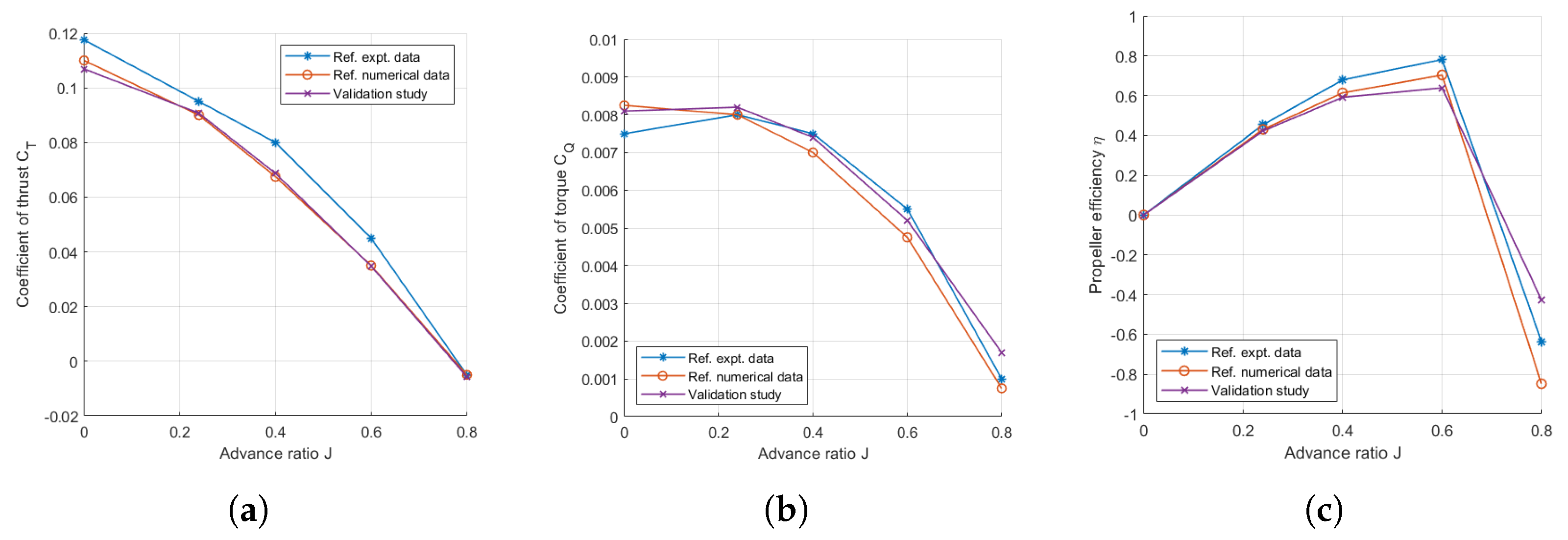
We see a good agreement between the reference and validation data across the given range of advance ratios as seen in Figure 4. The numerical results for $C_T$ from the reference data and the validation study match closely, while the $C_Q$ results from the validation study lie between the reference numerical and reference experimental results in the region of $\eta$∼ 0.5–0.6, where the main study of this paper will operate. Omitting the J = 0.8 condition, where the propeller yields net drag and negative propeller efficiency, the $C_T$ values from the validation study differ from the reference numerical data by <1.5% and the $C_Q$ values differ by <5%, which is sufficient to use in the following framework in this paper since the reference torque values also include hub and shaft influence as well. This validates the numerical setup to determine the propeller performance and can be used to simulate the propeller slipstream.

3.2. Baseline Performance of the Propeller to Be Used in the Main Study

The baseline performance of the Clark–Y–based propeller to be used in the main study is recorded in Figure 5. The numerical solution is deemed to have achieved a statistically stationary state after the mean of $C_T$ and $C_Q$ does not vary by more than 1% for ten rotations of the propeller. The propeller performance is calculated after achieving a statistically stationary state and the mean results of the last ten rotations are reported. To determine the net thrust requirement of the DEP configuration, an estimate from a study conducted on the same UAV airframe considering the average $C_D$ and a thrust–to–drag ratio of 1.25 indicates that each propeller should deliver a thrust of 84.80 N to maintain level cruise [28,29]. For a tip speed not exceeding M = 0.5 and a freestream velocity of 100 km/h, the corresponding operating condition is found to be J = 0.5833 and n = 6250 RPM, respectively, with an efficiency of $\eta$ = 0.5393. Since the validation study shows that the rotating propeller approach that will be used behaves well in this range of propeller efficiency, this operating condition of the propeller can be used in the present study. It is to be noted that no nacelle attachments and wing–propeller structural members have been considered in this study as the focus is mainly on the wing–propeller aerodynamic interactions.

3.3. Preliminary Study to Understand Propeller–Wing Interaction

We begin our framework with four representative DEP configurations to obtain a preliminary understanding of propeller–wing interaction using the modified actuator disk approach as described in Section 2.4. This part of the study is only to gain insight into the performance of configurations that are prevalent in consideration in academia and industry. To create such representative configurations, the same UAV airframe that will be used in the main study will also be used here. 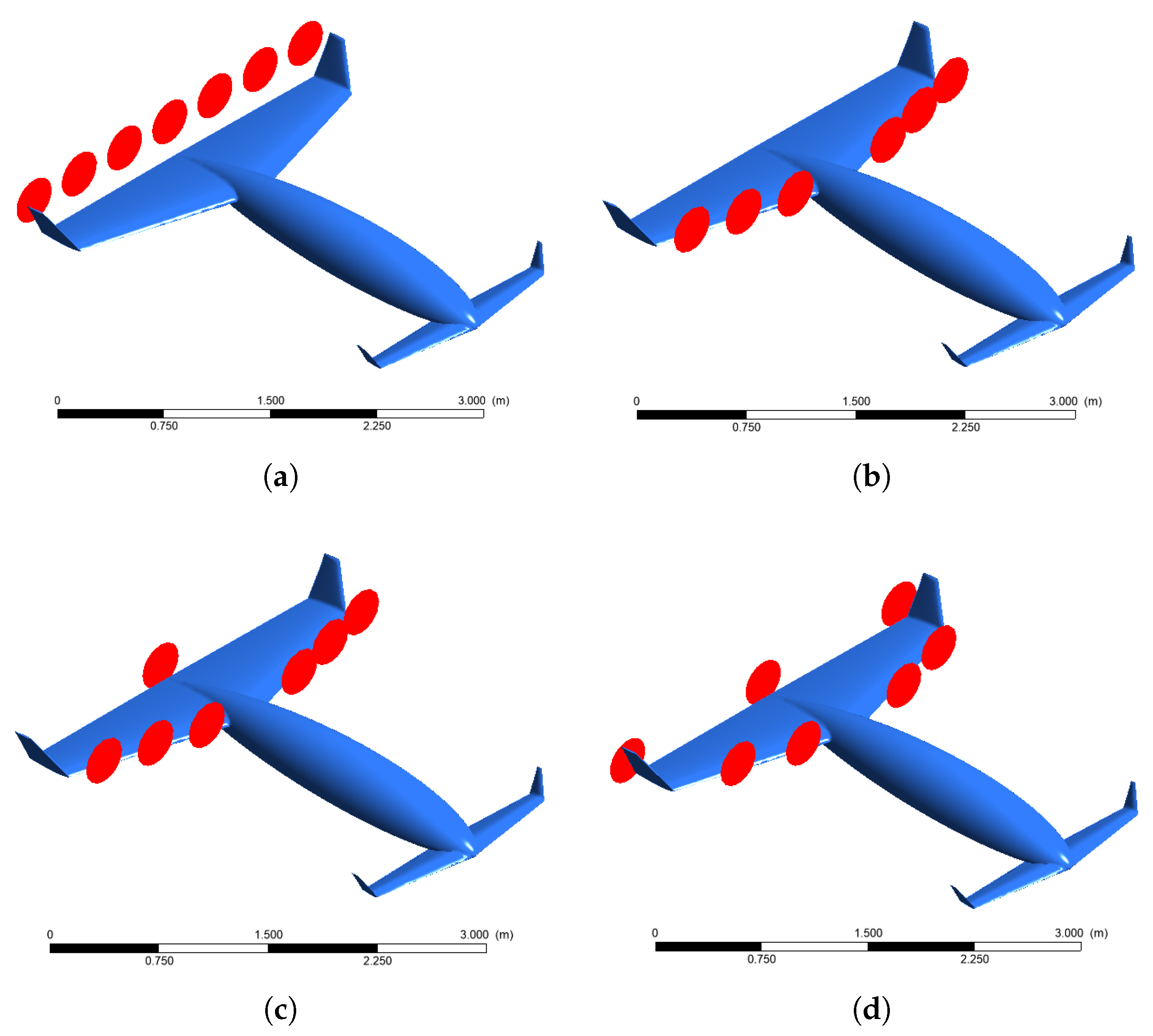This preliminary study performed using the modified actuator disk approach is conducted by authors separately [27,28,29] and yields some interesting results in terms of the change in $C_L$ and $C_D$ that motivate us to pursue the main study. We consider the following four DEP configurations for the preliminary study–pushers, tractors, tractors with a tail rotor, and tractors with a tail rotor and two tip rotors, as seen in Figure 6. It is to be noted that the preliminary study only serves as motivation to pursue the main study in this paper and is thus introduced to the reader to add context to the main study that will follow. The results of the main study are not taken from the preliminary study but the key insights are, such as the choice of configurations to investigate in detail, the range of angles of attack of interest, the requirement of vertical offsetting of propellers, and the effect of swirl in the actuator disk approach, to list a few.

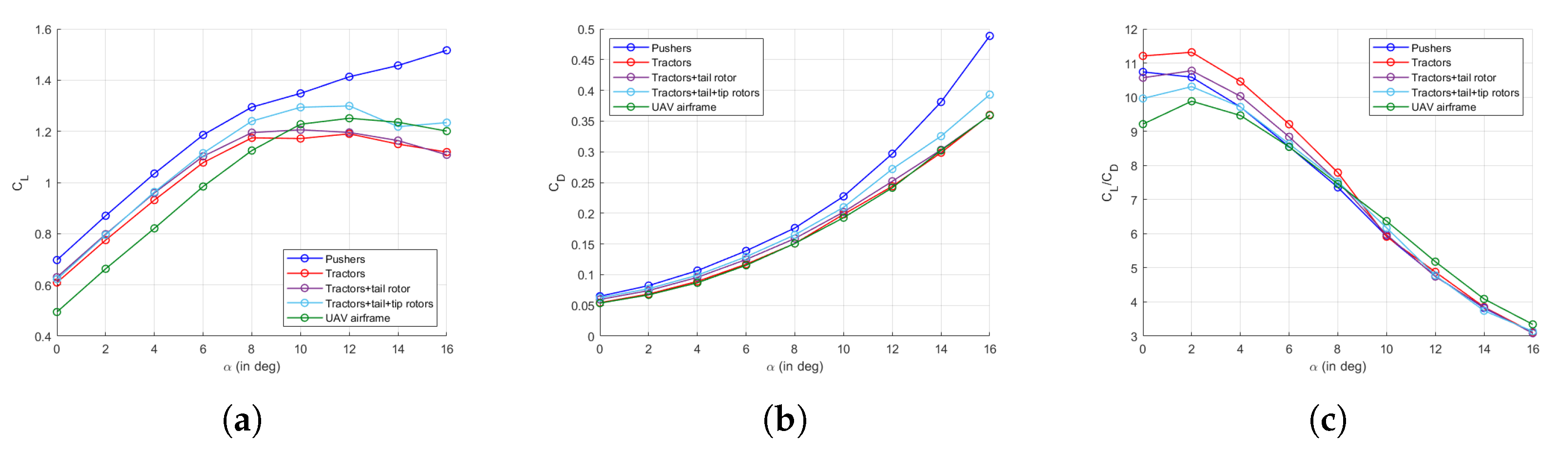
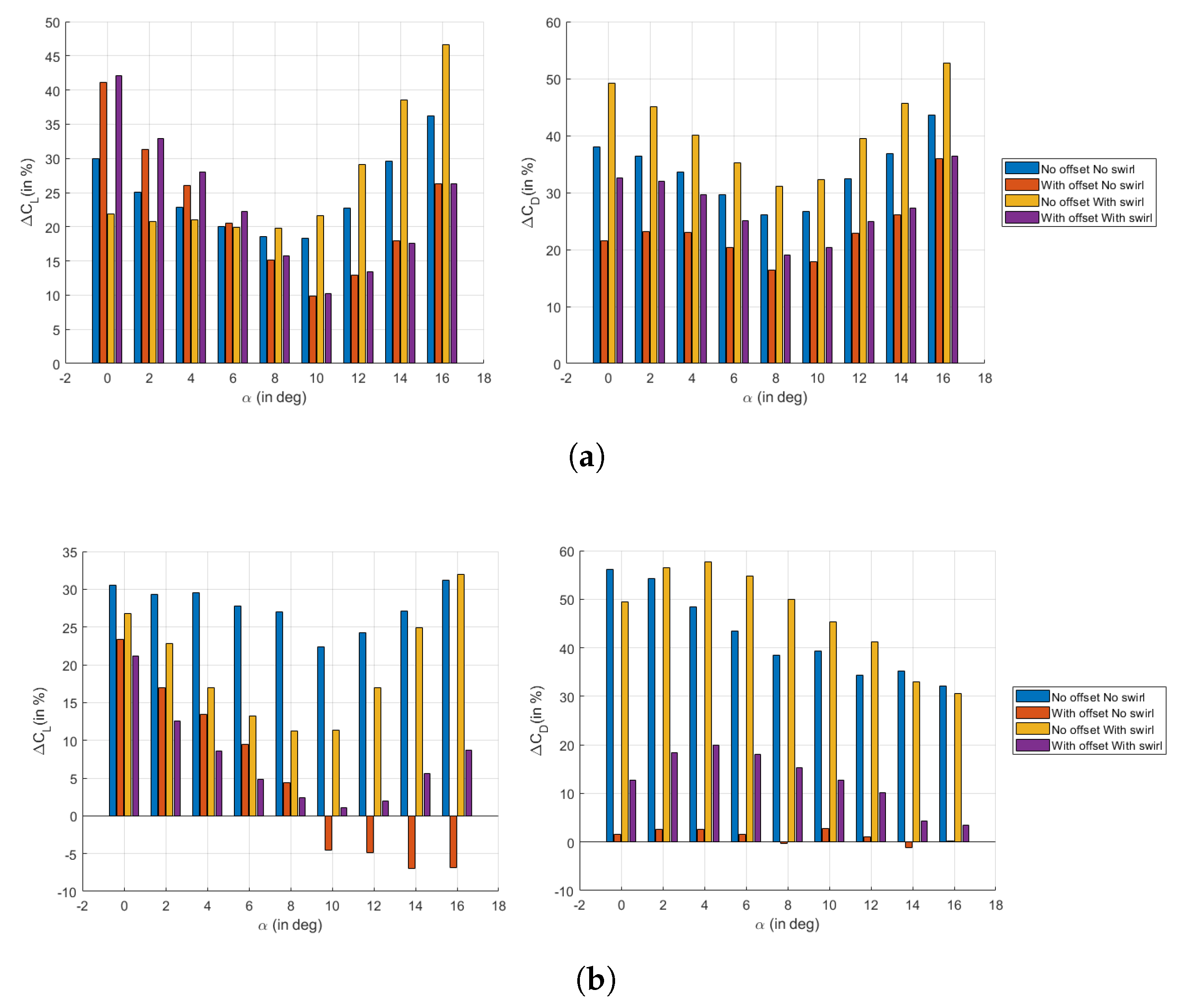
The aerodynamic characteristics of the preliminary configurations are computed and shown in Figure 7. The configurations are tested over $\alpha$ = 0${}^{\circ }$–16${}^{\circ }$ at $U_{\infty }$ = 100 km/h. The highest lift is obtained, in order, by the pushers, tractors with a tail rotor and two tip rotors, tractors with a tail rotor, and tractors. Thus, the highest difference in the lifting capacity is between the pushers and tractors. The configurations that offer the best aerodynamic efficiency are, in order, tractors, tractors with a tail rotor, tractors with a tail rotor and two tip rotors, and pushers, with marginal differences in their results. We also see that the configurations with offset always outperform those without offset and thus we shall use this vertical offset for the propellers in the main study as well. We again observe that the highest difference in efficiency is between the pushers and tractors, which motivates us to investigate these two configurations in detail in the main study. However, the outperformance of a configuration over the others could be dependent on various factors, such as the number and relative placement of propellers, desired thrust–to–drag ratio, etc., which can be studied separately by varying one of the parameters at a time using the unsteady solver.

We see a local minimum in the change in $C_L$ and $C_D$ in the range of 9${}^{\circ }$–10${}^{\circ }$ for these DEP configurations as seen in Figure 8. Hence, the range of $\alpha$ = 8${}^{\circ }$–14${}^{\circ }$ is chosen for the main study to investigate this in greater detail. The presence of a modeled swirl in the propeller slipstreams using the modified form of the actuator disk model produced significantly different results for the configurations as the swirl causes the reattachment of the separated flow back to the wing surface, allowing lift retention for extended angles of attack. Thus, the main study will include swirl effects in the slipstreams for the modified actuator disk approach. It is also evident from the preliminary study that both the lifting capacity and aerodynamic efficiency of the UAV are improved by the addition of the DEP configurations to the UAV airframe.

We are now motivated to investigate the pusher and tractor configurations in further detail when augmented to the UAV airframe at a vertical offset as the preliminary study provides only a time–averaged simplified solution. To understand the resolved flow physics in the proximity of the wing surface occurring due to the DEP configurations, we need to employ the use of an unsteady eddy–resolving numerical scheme, which is being carried out in the main study.

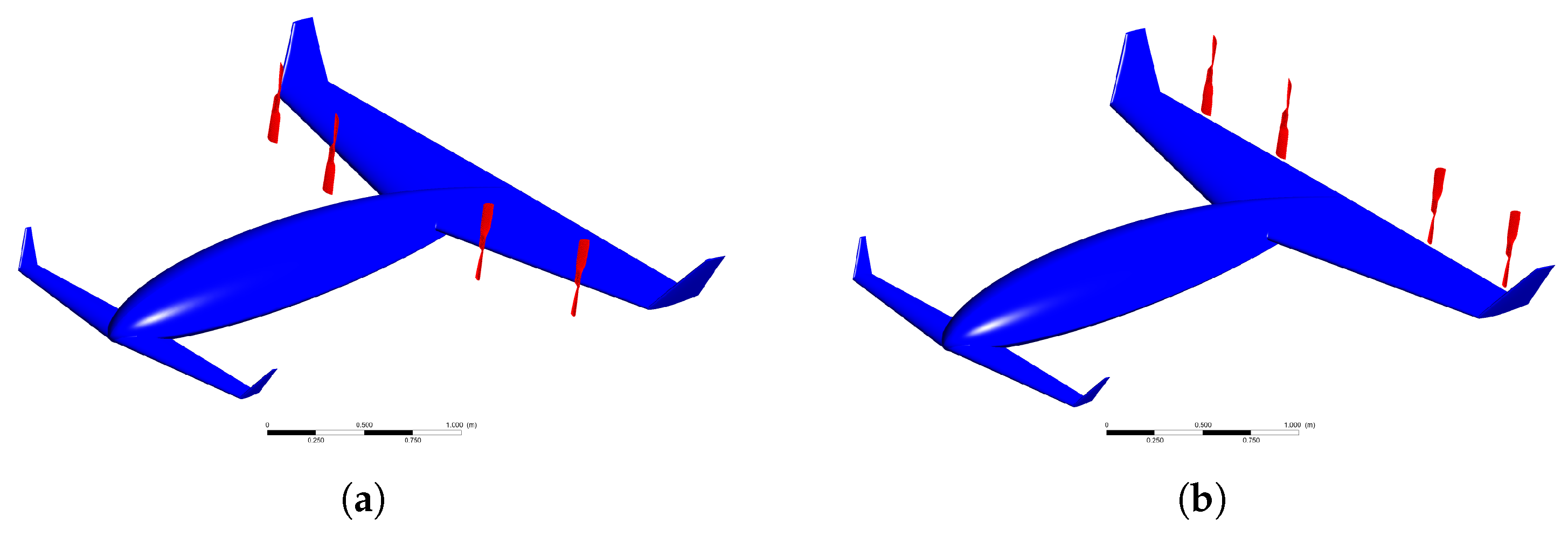
3.4. Main Study of the Pusher and Tractor DEP Configurations

Based on the results of the preliminary study, the pusher and tractor configurations are two DEP configurations that exhibit differing results with an increasing angle of attack due to the suction and blowing effects of their propeller slipstreams, respectively. So, we now investigate these two DEP configurations for the main study of this paper using the rotating propeller approach and later using the modified actuator disk approach to understand their performance in greater detail. We shall now use the rotating propeller approach that has been validated to conduct the main study of this paper, where we investigate the aerodynamic performance of the two DEP configurations shown in Figure 9.

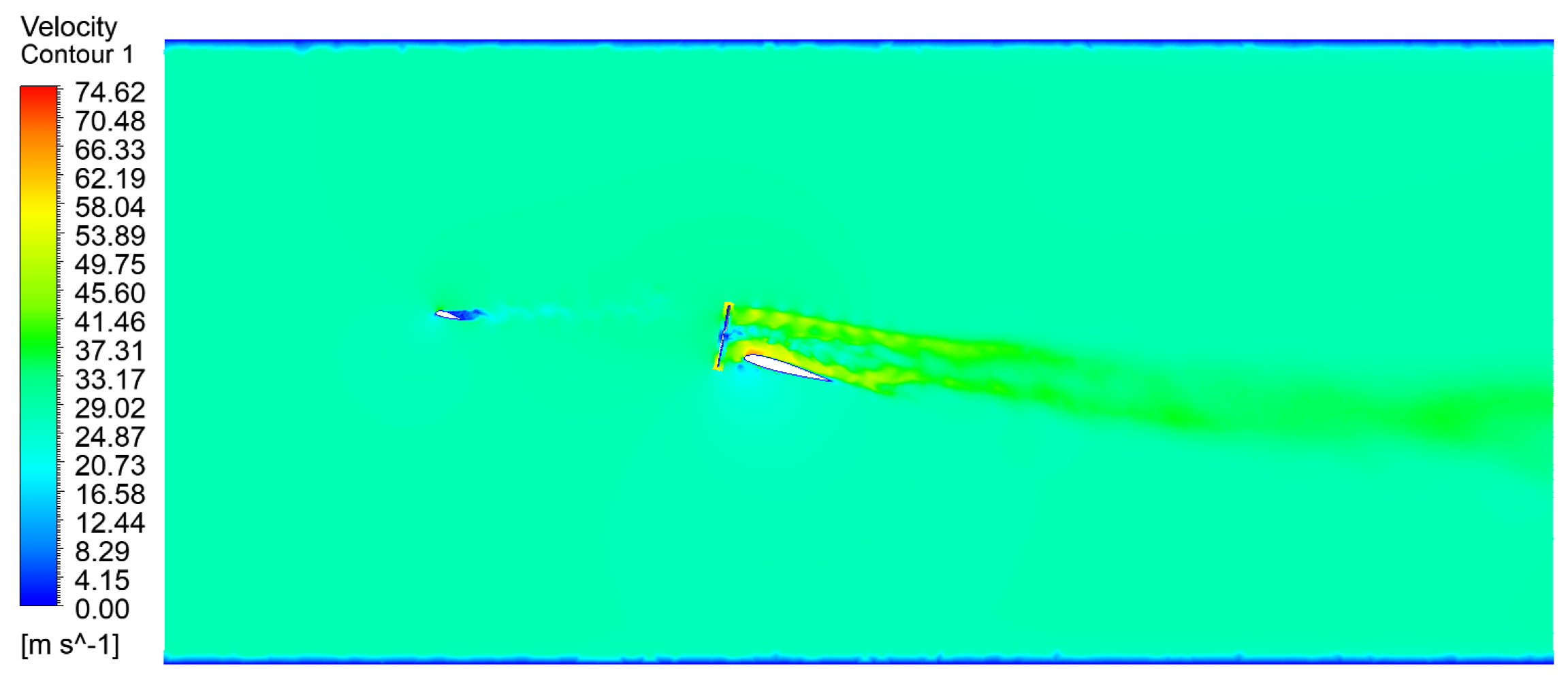
Figure 10 shows the instantaneous velocity contours drawn over the cross–section of the domain and located normal to the plane of the first propeller for the tractor configuration at $\alpha$ = 10${}^{\circ }$ after the solution has achieved a statistically stationary state. The cross–sections of the canard and main wings are visible in the image. We observe that the main wing interacts with the slipstream of the propeller placed ahead of its leading edge and the wake of the canard wing. Since the domain is sized considering replicating the current setup in a wind tunnel in the future, the effect of the walls of the domain is also minimal as seen in the velocity contours. The propeller slipstreams are allowed enough distance downstream of 13D–15D, as described earlier, to develop spatially until the outlet of the domain.

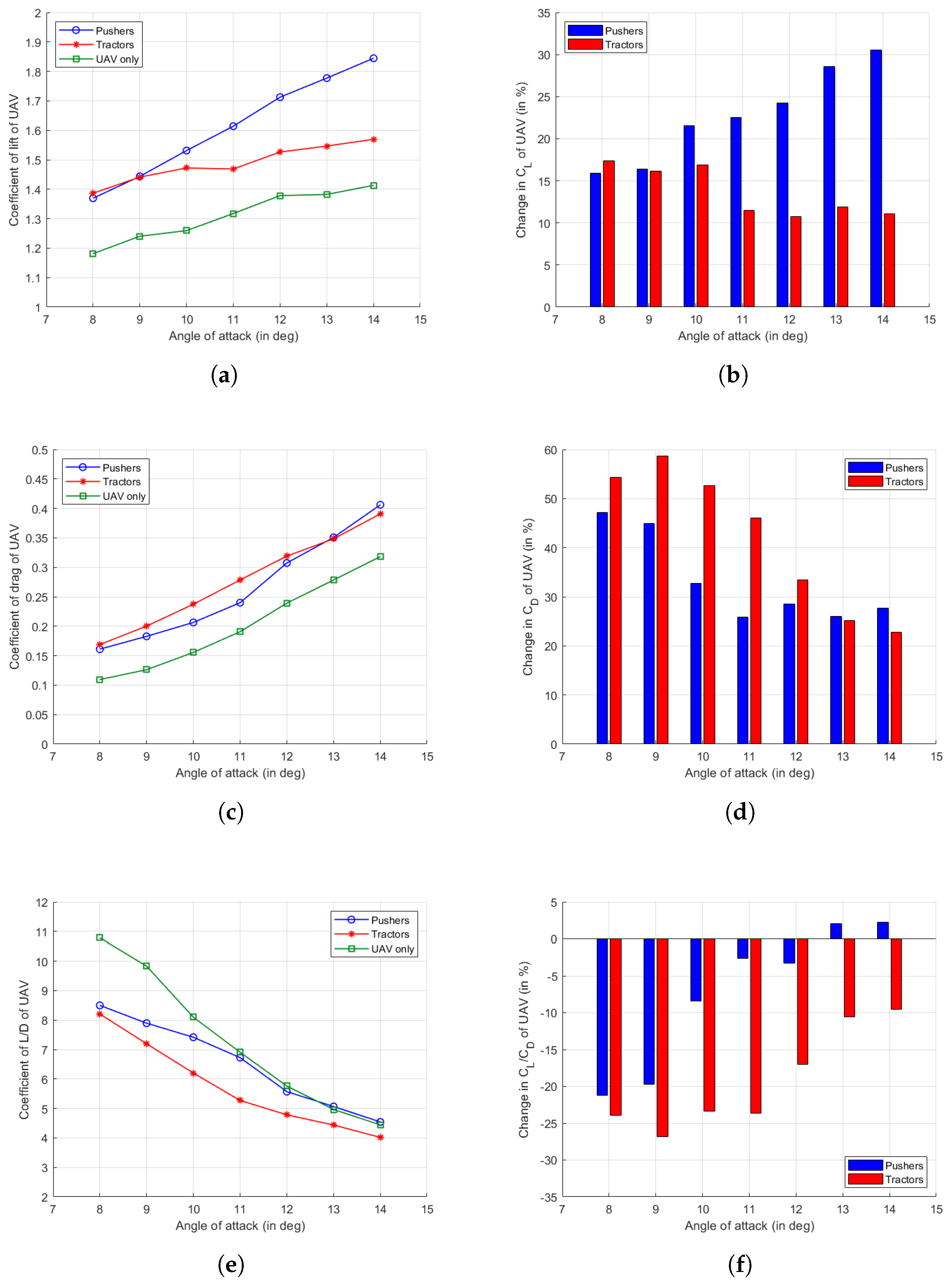
See Figure 11 for the comparison of coefficients of the lift and drag of the UAV airframe with and without the propeller configurations for $\alpha$ = 8${}^{\circ }$–14${}^{\circ }$. The UAV airframe stalls at approx. 12${}^{\circ }$. It is observed that the drag experienced by the UAV with the tractor and pusher configurations is higher compared to the UAV airframe due to the increased dynamic pressure by the propellers. The lifting capacity, too, increases for both configurations due to the interaction with the propeller slipstreams, although unequally more for the pusher configuration. The change in $C_L$, $C_D$, and $C_L/C_D$ for the DEP configurations is defined in Equation (2).

$$\begin{array}{c}\mathsf{\Delta }{C}_{L-DEP}=\frac{C_{L-DEP}-C_{L-UAV}}{C_{L-UAV}}\times 100\%\hfill \\ \\ \mathsf{\Delta }{C}_{D-DEP}=\frac{C_{D-DEP}-C_{D-UAV}}{C_{D-UAV}}\times 100\%\hfill \\ \\ \mathsf{\Delta }{C}_{L/D-DEP}=\frac{C_{L/D-DEP}-C_{L/D-UAV}}{C_{L/D-UAV}}\times 100\%\hfill \end{array}$$

(2)

We observe that the average change in $C_L$ and $C_D$ for the tractors is 13.66% and 41.85%, respectively. On the other hand, we see that the changes for the pusher configuration of $C_L$ and $C_D$ are 22.82% and 33.25%, respectively. The difference in the $C_L$ curves of the pusher and tractor configurations widens as $\alpha$ increases as the suctioning action of the pusher propellers allows the UAV to retain its lifting capacity even at higher angles of attack. The injection of momentum by the tractor propellers’ slipstreams into the boundary layer of the wing proves to be insufficient to maintain boundary layer attachment to the wing surface at higher angles of attack. Hence, there is no corresponding increase in the lifting capacity for the tractors as $\alpha$ increases. The drag experienced by the configurations increases sharply as the UAV stalls, but the marginal change in the drag reduces with $\alpha$.

To estimate the net effect of the propeller placement on the aerodynamic performance of the UAV, we look at the aerodynamic efficiency of the UAV ($C_L/C_D$). We see that the average deterioration in $C_L/C_D$ of the UAV by the tractors is 19.27% whereas the pushers perform better at 7.28%. At smaller angles of attack, the tractors offer a similar lifting capacity to the pushers but they offer no advantage as the lift wears off as we approach stall while the drag continues to increase due to the increasing form drag of the UAV. At higher angles of attack in the given ambient conditions, the tractors are unable to avoid the separation of the boundary layer, resulting in the enlargement of the recirculation bubble toward the trailing edge of the wing. Thus, the tractors perform considerably worse than the pushers at high $\alpha$ whereas the pushers offer a marginal improvement in the aerodynamic efficiency beyond stall. However, operating the pusher configuration at or beyond stall to achieve little to no depreciation of aerodynamic efficiency is inadvisable as the absolute values of aerodynamic efficiency can be infeasible to practically operate while requiring a high thrust capability to overcome the increased drag experienced by the aircraft.

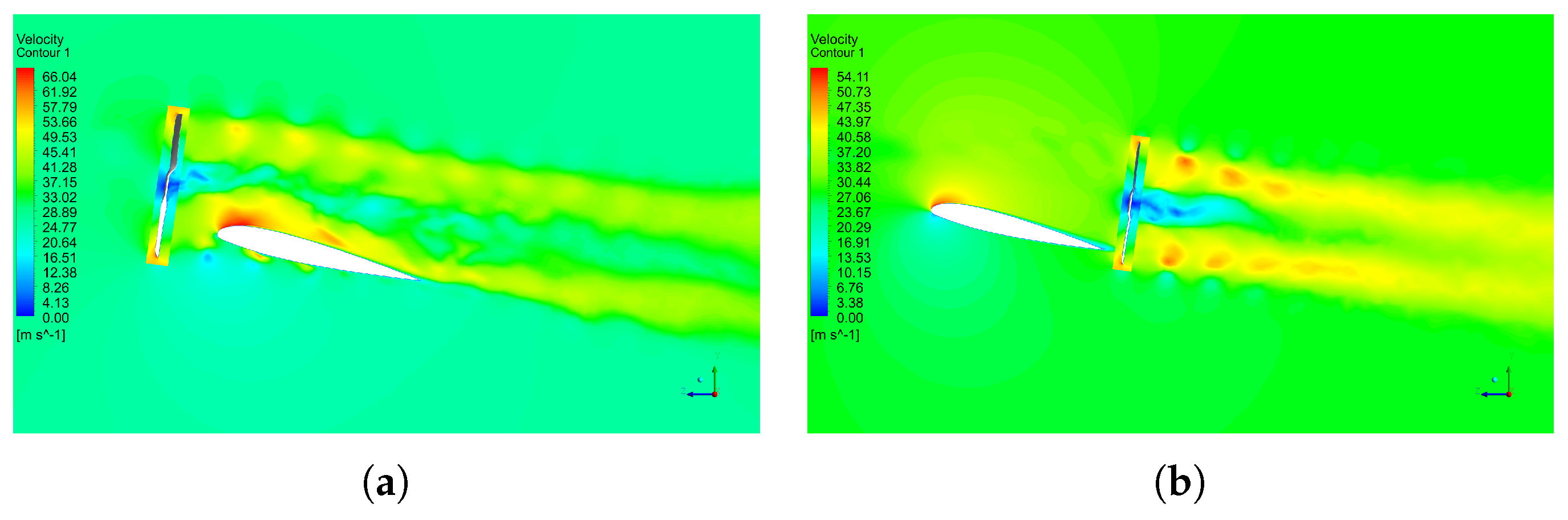
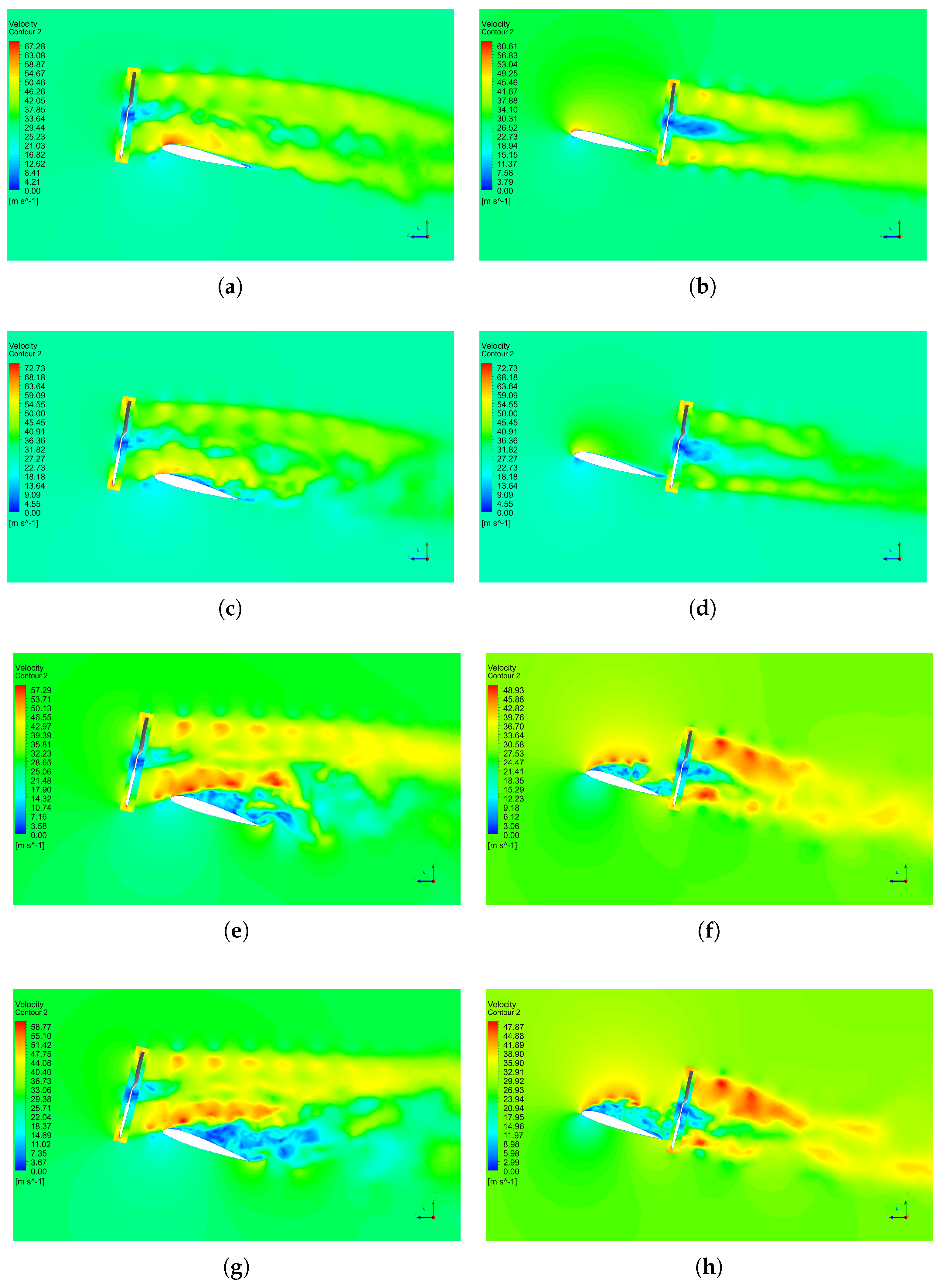
To visualize the aerodynamic interaction of the propeller slipstreams with the main wing, see Figure 12 and Figure 13. The velocity contours on the planes normal to the first and second propellers passing through their axes for both configurations are shown. There is a demarcation of local flow domains due to the use of rotating sub–domains. The insight of placing the propellers at a vertical offset to encourage the interaction of the propeller slipstreams primarily with the suction surface of the main wing from the preliminary study is seen clearly in the velocity contours. The implementation of DES for turbulence modeling allows us to clearly visualize the eddies shed by the blades of the propellers and their interaction with the UAV. We see that the tip–vortices shed by the propeller blades ahead of the leading edge wash over the suction surface of the main wing. In the case of tractor configuration, we see that the lower half of the slipstream flows mainly over the suction surface whereas the upper edge of the slipstream is 0.43c–0.45c away from the wing surface.

We see that the slipstreams of the tractor propellers tend to diffuse out more with an increasing angle of attack due to the action of the freestream on it. For the pusher configuration, we see that the flow over the wing surfaces is much smoother as compared to the tractor configuration since the flow instabilities are essentially suctioned into the propeller, thus stabilizing the flow. At higher angles of attack, as we go farther from the root of the main wing, due to the increased influence of the wake of the canard and the stall of the main wing, the flow increasingly separates for both propeller configurations. However, the separation of the boundary layer and consequent formation of the recirculation bubble are delayed for the pusher configuration compared to the tractor configuration. This is again due to flow smoothening by the suction action of the pusher propellers’ flow intake.

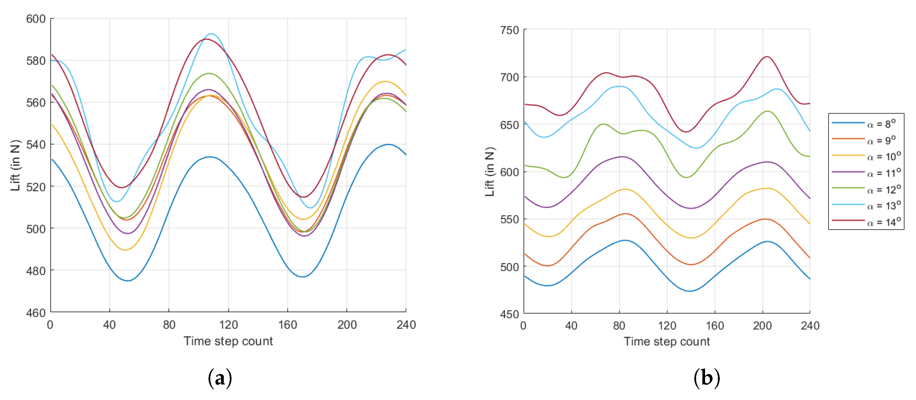
Let us look at the oscillating lift curve of the UAV–propeller configurations as shown in Figure 14. We record the instantaneous values of the lift of the configurations (in N) at every time step for one complete rotation of the propeller after the solution has achieved a statistically steady state. The average amplitude of this oscillating lift curve across the angles of attack under consideration for the tractors is ∼36.68 N. For the pusher configuration, we see that the vertical offset of the propellers allows the separated boundary layer to stay closer to the wing surface as the propeller axes are parallel to the main wing’s chord. This results in a smoother flow over the wing and maintains an average amplitude of ∼30.74 N of the instantaneous lift curve, thus yielding a more predictable and smoother instantaneous lift response from the wing.

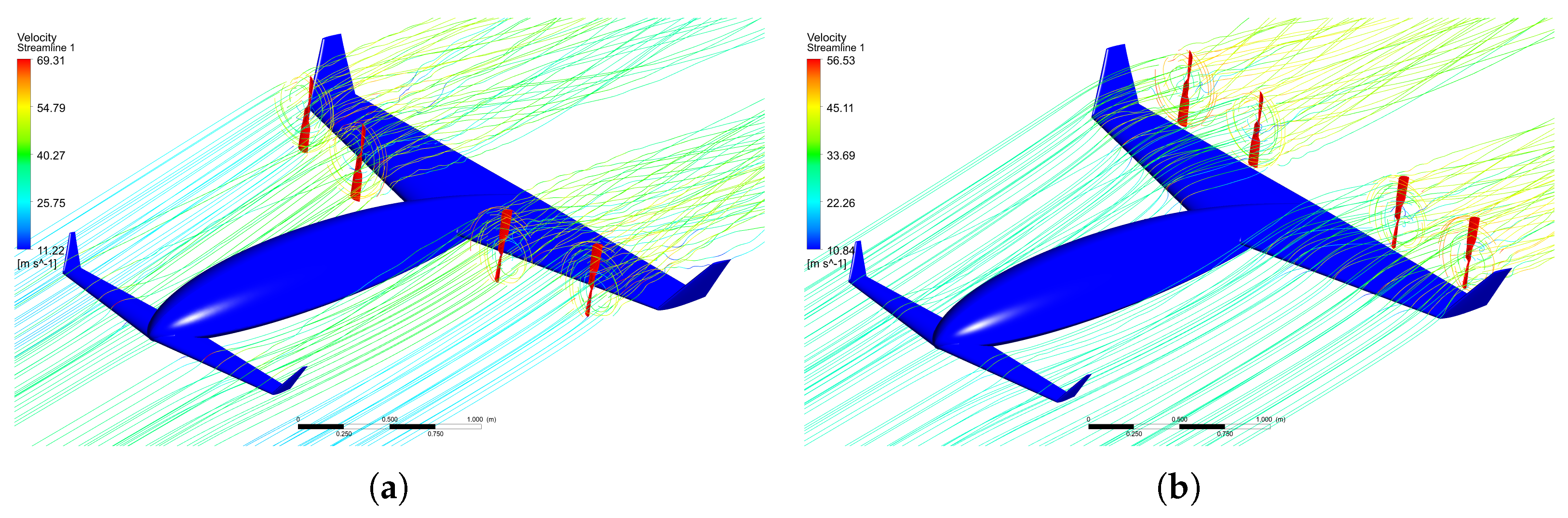
Thus, the proposed framework indicates a clear preference for the pusher configuration for the placement of propellers in such a distributed propulsion system considering it can not only sustain lift at higher angles of attack, i.e., beyond stall of the airframe, but also maintain good aerodynamic efficiency as compared to the tractor configuration. This is also evident from the streamlines over the wing surfaces as seen in Figure 15. The stall is thus gentle for the pusher configuration, allowing for a better control of the aircraft due to an extended flattened lift curve compared to the tractor configuration. Since we have established that the pusher configuration is preferable over the tractors using an unsteady solver, which requires large computational resources, we will now look at estimating the aerodynamic performance of these configurations using a simpler and less computationally expensive steady–state modified actuator disk approach, which was also used in the preliminary study.

3.5. Comparison of Results from Rotating Propeller and Actuator Disk Approaches

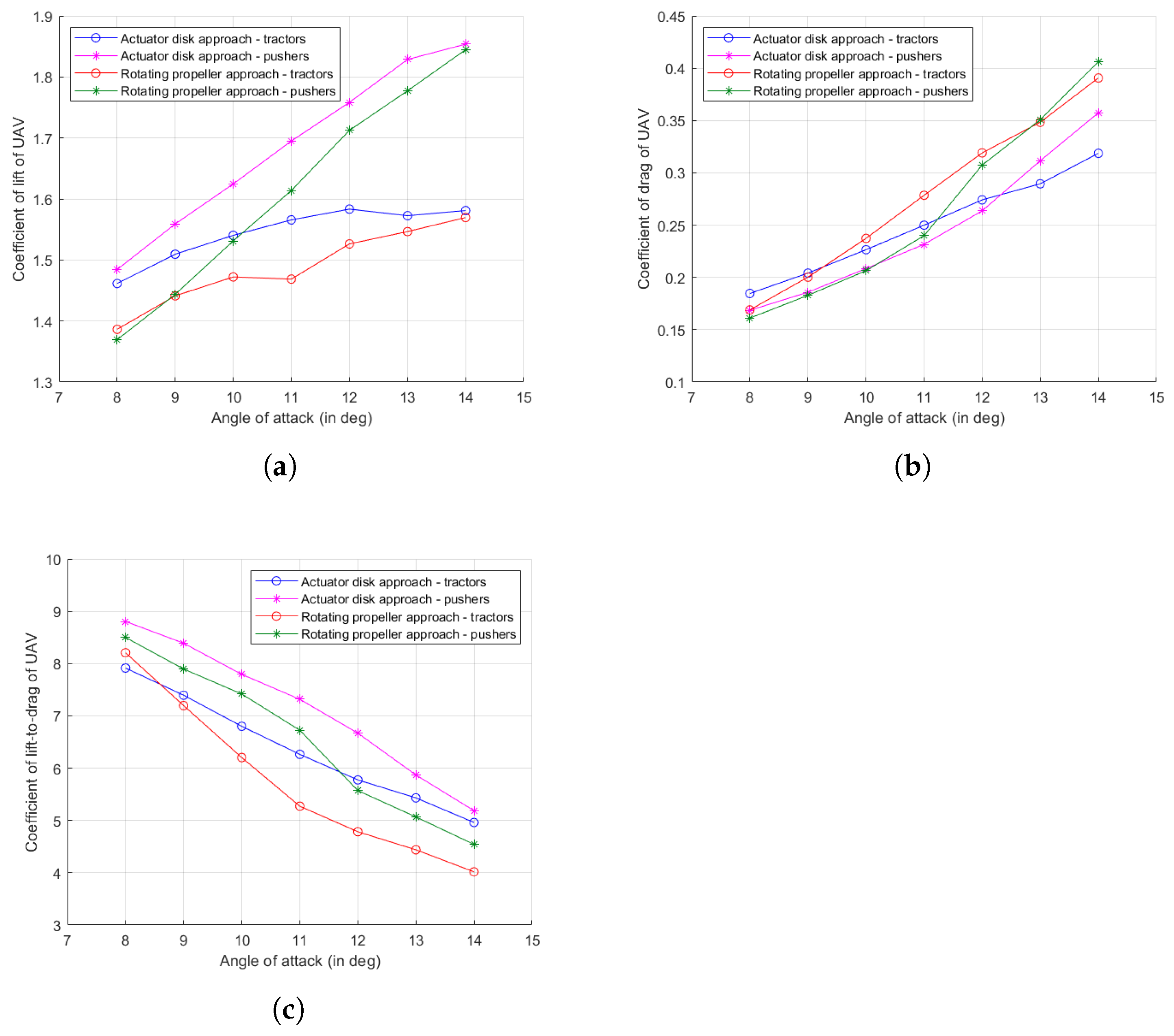
We now compare the results obtained from the two numerical approaches for the UAV–propeller configurations to estimate the difference in numerical results, i.e., from modified actuator disk–based and rotating propeller approaches. See Figure 16 for the comparison of $C_L$, $C_D$, and $C_L/C_D$ obtained from the two numerical approaches. We see an overall concurrence of the trend of the aerodynamic performance of the DEP configurations between the two approaches. The lift curve corresponding to the modified actuator disk approach for the pusher configuration captures the ability of the pushers to retain their lifting capacity at higher angles of attack. The difference in the results obtained from the two numerical approaches is quantified as the absolute difference in the value obtained from the modified actuator disk approach and the rotating propeller approach, normalized with the latter, as given in Equation (3). The average of the differences in results from the two approaches is presented in

Table 3. Difference in the results from the modified actuator disk approach with regard to rotating propeller approach.

Aerodynamic Characteristic	Tractor Configuration (in %)	Pusher Configuration (in %)
$\delta C_{L-AD}$	3.93	4.80
$\delta C_{D-AD}$	10.78	6.88
$\delta C_{L/D-AD}$	14.48	10.50

.

$$\begin{array}{c}\delta C_{L-AD}=\frac{|C_{L-AD}-C_{L-RP}|}{C_{L-RP}}\times 100\%\hfill \\ \\ \delta C_{D-AD}=\frac{|C_{D-AD}-C_{D-RP}|}{C_{D-RP}}\times 100\%\hfill \\ \\ \delta C_{L/D-AD}=\frac{|C_{L/D-AD}-C_{L/D-RP}|}{C_{L/D-RP}}\times 100\%\hfill \end{array}$$

(3)

Since we attempt to present a framework to estimate the aerodynamic performance of a DEP–enabled UAV–propeller configuration, we acknowledge that it may not always be viable to use computationally expensive numerical approaches such as LES or DES for this task; hence, one way to begin the design process would be to start with the modified actuator disk approach. In such a case, the difference in results of the two approaches needs to be considered to account for the possible error when using the modified actuator disk approach as opposed to a rotating propeller approach when designing a distributed propulsion system. These values indicate that the modified actuator disk approach can estimate the lift produced by the configurations with a reasonable accuracy of <5% but requires a wide error tolerance of ∼10% in the estimation of drag experienced by the UAV–propeller configurations. This further worsens the estimate from the actuator disk approach of the aerodynamic efficiency to ∼15%. Since the rotating propeller profile approach uses an unsteady scheme with fewer modeling assumptions than the actuator disk approach in determining the velocity field, eddy formation, shedding and dissipation, interaction of eddies with freestream and airframe, etc., the aforementioned error values highlight the loss in accuracy of results due to the assumptions made for the steady–state results used in the modified actuator disk approach in designing a DEP configuration. Thus, it is possible to estimate the aerodynamic performance of the DEP configurations using both numerical approaches but the flow physics is more accurately captured and visualized using the unsteady rotating propeller approach due to its ability to spatio–temporally resolve the eddies shed by the propeller blades and their subsequent interaction with the UAV airframe.

4. Conclusions

Distributed electric propulsion is implemented onto a novel canard aircraft and a conceptual framework used to design an optimal DEP for a given airframe is presented. A preliminary study of four DEP configurations that are prevalent in academic and commercial studies is presented. Based on the changes in the lifting capacity, the effect of swirl, the vertical offset of propellers, etc., on the DEP configurations, key insights are drawn and the tractor and pusher configurations are chosen for further analysis in the main study. The blowing versus the suction effect of the propellers is thus compared. In the main study, two numerical approaches are used to estimate the performance of the DEP configurations: modified actuator disk– and rotating propeller–based approaches. The turbulence is simulated using the DES eddy viscosity model to capture the spatio–temporal interaction of the eddies shed by the propellers over the wing.

The preliminary study identifies that the pusher and tractor configurations among the four most commonly seen DEP configurations are of interest due to a significant difference in their lifting capacities and aerodynamic efficiencies with an increasing angle of attack. This is achieved using a modified actuator disk approach. The vertical offset of the propellers allows for their slipstreams to interact primarily with the suction surface of the main wing, thereby reducing a potential increase in drag due to increased dynamic pressure. The introduction of swirl in the slipstreams through the modified actuator disk approach extends the lift curve of the aircraft by delaying stall. Using these insights, the main study of this paper is undertaken for the pusher and tractor configurations, first using the unsteady rotating propeller approach.

We observe in the main study that the pusher configuration delivers an unequally higher lifting capacity than the tractors due to its ability to delay boundary layer separation from the wing surface. The suctioning effect of the pushers prevents the formation of a separation bubble for a wide range of angles of attack, thereby performing better than the tractors. Although the tractors introduce momentum into the boundary layer of the wing, they prove to be insufficient in preventing stall–induced flow separation. The performance of the two configurations is similar for smaller angles of attack but is significantly different later. The tractors severely deteriorate the lift–to–drag ratio of the DEP configuration compared to the pushers. The flow smoothening by the pushers also results in a smaller amplitude of the instantaneous oscillating lift curve of the UAV. Subsequently, the steady–state RANS–based modified actuator disk approach is also used to compare the two DEP configurations considering that the DES–based rotating propeller approach requires large computational resources. Since the RANS–based approach includes more assumptions in modeling a highly turbulent 3D flow expected in such DEP configurations, the error in its accuracy compared to the rotating propeller approach is noted when designing/fitting a DEP configuration. Nevertheless, the modified actuator disk–based approach still convincingly captures the overall trend of the aerodynamic performance of the two configurations and thus the outperformance of the pushers over the tractors.

This paper presents a conceptual framework to investigate the propeller–wing interaction for a given UAV airframe when coupled with different propeller configurations to design an optimal propeller configuration. This analysis can now be extended to augment any given UAV airframe with any DEP. This translates to exploring various viable electric aircraft for passenger and cargo air travel. When presented with a choice of pushers or tractors or a combination of the two, the present study offers a guide to quantify the expected performance of an integrated DEP configuration. A different number of propellers and their vertical and lateral placements can now be tested with a given airframe in a modular approach presented here to investigate all possible DEP configurations. Complex configurations such as tail–mounted and VTOL configurations can also be investigated. The authors intend to further investigate these DEP configurations using an experimental approach in a wind tunnel to compare it with the aforementioned numerical approaches.