Analyzing Multi-Mode Fatigue Information from Speech and Gaze Data from Air Traffic Controllers

Abstract

In order to determine the fatigue state of air traffic controllers from air talk, an algorithm is proposed for discriminating the fatigue state of controllers based on applying multi-speech feature fusion to voice data using a Fuzzy Support Vector Machine (FSVM). To supplement the basis for discrimination, we also extracted eye-fatigue-state discrimination features based on Percentage of Eyelid Closure Duration (PERCLOS) eye data. To merge the two classes of discrimination results, a new controller fatigue-state evaluation index based on the entropy weight method is proposed, based on a decision-level fusion of fatigue discrimination results for speech and the eyes. The experimental results show that the fatigue-state recognition accuracy rate was 86.0% for the fatigue state evaluation index, which was 3.5% and 2.2%higher than those for speech and eye assessments, respectively. The comprehensive fatigue evaluation index provides important reference values for controller scheduling and mental-state evaluations.

1. Introduction

Rapidly growing flight volumes have resulted in an increasing workload for air traffic controllers. Research shows that an excessive workload contributes to controller fatigue and negligence, leading to flight accidents [1]. Therefore, fatigue detection in controllers is an important means of preventing air traffic safety accidents.

The current research related to fatigue detection can be divided into two categories: subjective detection and objective detection. Compared to subjective detection methods, objective detection methods do not require subjects to stop their work, making objective detection methods more practical. Among them, objective detection can be divided into contact detection methods such as the ECG signal detection method [2] and the EEG signal detection method [3]. The contact detection method requires the controller to wear detection equipment, which is intrusive and may affect the controller’s control work. Therefore, the non-contact fatigue detection method is more suitable for the controller’s work scenario.

Controllers need to frequently use radiotelephony in their daily work. Previous studies have shown that the frequency of instruction errors in radio telephony are important fatigue characteristics [4]. Therefore, radio telephony reflects the current fatigue status of the controller. The radio telephony fatigue feature detection method is a very practical and effective detection method. Li [5] conducted a speech-fatigue test on members of an American bombing crew, and found that the pitch and bandwidth of their speech signals showed significant changes after a long flight. When the human body is in a state of fatigue, speech signals will exhibit a decrease in pitch frequency and changes in the position and bandwidth of the spectral resonance peak [6]. Wu [7] extracted MFCC features from radiotelephony communications and proposed a self-adaption quantum genetic algorithm, but their ability to describe audio with only MFCC is limited. A multi-angle description of speech should use multiple features. Kouba [8] discussed the use of a contact method combined with speech, which can more comprehensively present the current fatigue state of the controller through two modalities. However, the collection of EEG information is time-consuming and can affect the progress of control work. Vasconcelos’s research [9] shows that low elocution and articulation rates mean that the pilots are in a fatigue state, and it shows that recognizing fatigue states through speech recognition is feasible. Studies have shown that various types of sound quality characteristics reflect the sound quality changes before and after fatigue.

Traditional speech signal processing usually relies on linear theory. Based on their short-term resonance characteristics, speech signals can be simulated as a time series composed of an excitation source and a filter to construct a classic speech signal excitation-source–filter model [10]. These signals can be described using various model parameters for further procession and analyses. Recently, speech-signal research has led to scholars concluding that the process of generating speech signals is a nonlinear process; that is, it is neither a deterministic linear sequence nor a random sequence, but rather a nonlinear sequence with chaotic components. Therefore, traditional linear filter models cannot fully represent the information contained in speech signals [11]. A nonlinear dynamic model of a speech signal is generally constructed using a delay-phase diagram that is obtained by reconstructing the time series of a one-dimensional speech signal in the phase space [12]. Previous studies also showed that the fatigue state of the human body influences the phase-space track of speech, especially the degree of chaos in its phase space [13]. Considering the respective characteristics of both linear and non-linear speech features, this paper extracts linear features and non-linear features for air talk at the same time, and fuses the two types of features to create the features of controller’s fatigue speech.

In the field of fatigue recognition, the face is considered an important information system which contains the fatigue status of the subject. Many scholars have considered information about the eye in fatigue detection research. Wierwille [14] analyzed the relationship between a driver’s eye closure time and the collision probability in experiments on driving fatigue, and found that eye closure time can be used to characterize fatigue. The US Transportation Administration also conducted experiments investigating nine parameters including blink frequency, closure time, and eyelid closure, and demonstrated that these characteristics can also be used to characterize the degree of fatigue. Jo et al. [15] proposed an algorithm for determining the eye position of drivers based on blob features. Some scholars applied principal-components analysis [16] and linear discriminant analysis [17] to extract ocular features, and finally judged the fatigue state of a driver using a support vector machine (SVM) classifier. It can be seen that eye features have important reference value in fatigue recognition. When the controller stops sending radio telephony, we use his eye features to determine the current fatigue state. To this end, we perform feature-level fusion and decision-level fusion on the controller’s voice features and eye features.

Multi-source data fusion can provide the model with richer detailed features. Compared with previous research that relied entirely on radio telephony or facial data, a multi-source feature fusion approach is adopted in this study by extracting various speech features from radio telephony and integrating speech features with facial features, proposing a method for controller fatigue recognition through multi-source feature fusion. In our model, different speech features are fused at the feature layer and passed through a classifier for speech fatigue feature recognition. The recognition results for eye fatigue characteristics and the recognition results for voice fatigue characteristics are fused at the decision-making level via a weighting method to obtain the best fatigue recognition results. In order to verify the effectiveness and robustness of our model, in the experimental part we collected data from a total of six controllers in tower control and approach control positions. In addition, our data collection experiment lasted for one week, and the data from each licensed controller can be divided into six periods, so the data obtained are sufficiently representative.

The main contributions of this work are listed as follows:

• This paper performs linear feature extraction and nonlinear feature extraction, respectively, for radio telephony, and uses FSVM to perform fatigue recognition for speech fusion features.
• In order to detect the fatigue status of the controller when he stops sending radio telephony, this paper extracts eye-fatigue-feature PERCLOS, and evaluates the fatigue status of the controller using a threshold method.
• This paper uses a weighting method to perform decision-making fusion based on the fatigue recognition results for voice features and facial features, and conducts experiments to verify the effectiveness and robustness of the model.

This paper is structured as follows: In Section 2, we introduced the multi-level information fusion model used in this paper, including the model’s feature extraction from data sources, feature fusion, fusion feature recognition, and the decision layer fusion process based on two types of recognition results. In Section 3, we introduced the controller fatigue feature extraction recognition experiment carried out in this paper, including the process of collecting fatigue data and the processing results according to the model used in this paper. The last part is our summary of this paper. Section 4 draws together our conclusions, demonstrating that the accuracy of our multi-level information fusion model is enhanced when processed using the FSVM classifier.

2. Methods

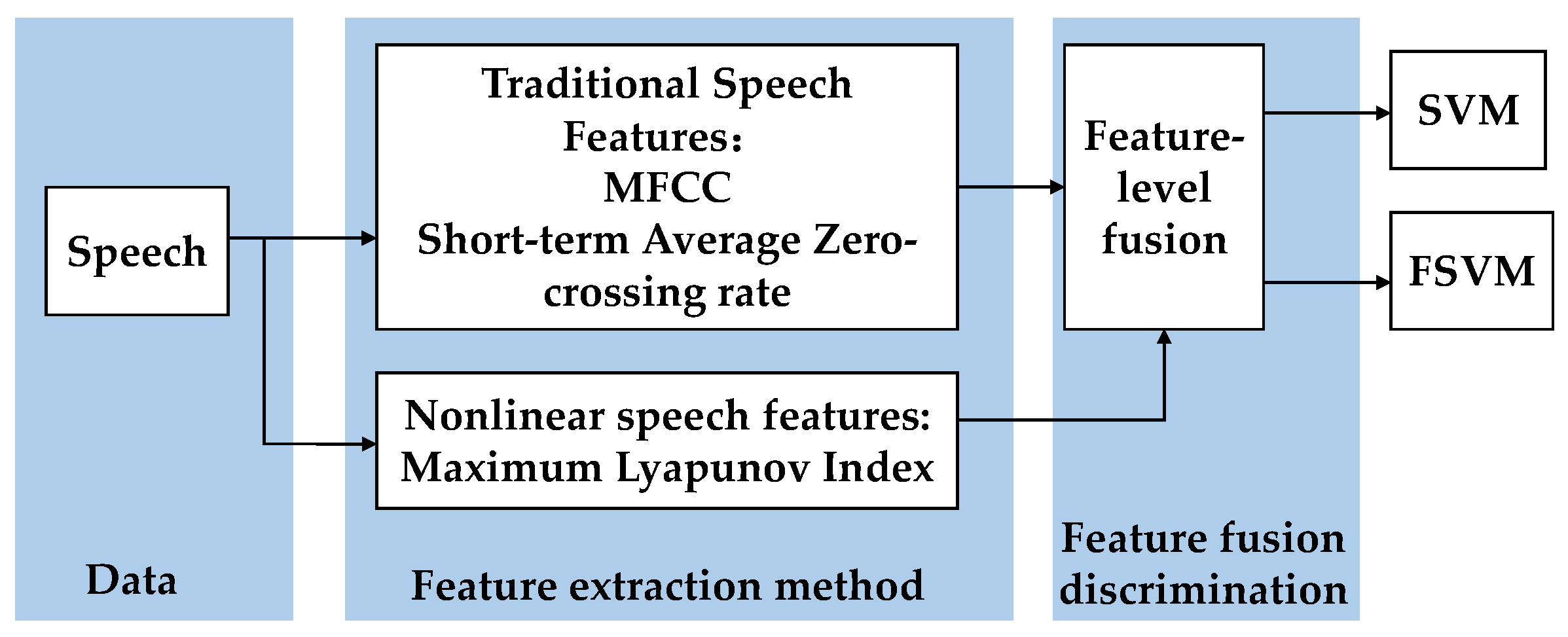
Currently, in the field of speech processing recognition, there are various speech features. We can divide them into three categories: spectral features, statistical features, and nonlinear features. We choose one from each category so that our data fusion can depict speech from three different perspectives. Here we extract the Mel frequency cepstral coefficient (MFCC), short-time-average zero-crossing rate, and maximum Lyapunov index. Based on the use of the percentage of eyelid closure over time (PERCLOS) as the eye features, feature fusion was applied to the features of the two types of data sources, and an evaluation index system was established.

The structure of the fatigue evaluation index is shown in Figure 1.

2.1. Speech Feature Classification Algorithm Based on the FSVM

In fatigue detection, the fuzzy samples in the feature space often lead to reduction of the classification interval and affect the classification performance of the classifier [18]. In practical applications, training samples are often affected by some noise. This noise may have adverse effects on the decision boundary of the SVM, leading to a decrease in accuracy. To solve this problem, this paper introduces the idea of a fuzzy system and combines it with an FSVM algorithm.

Here, the membership function is first introduced. A membership function is a concept in fuzzy sets that represents the degree to which each element belongs to a certain fuzzy set, with the degree value ranging between 0 and 1.The principle behind the algorithm in the FVSM is to add a membership function $\mu (x_i)$ to the original sample set $(x_i,y_i),i=1,2,\dots ,n$, so as to change the sample set to $\left\{x_i,y_i{\mu }_i(x_i)\right\},i=1,2,\dots ,n$. Membership function $\mu (x_i)$ refers to the probability that the $i$th sample belongs to the $y_i$ category; this is referred to as the reliability, where $0<\mu (x_i)\le 1$, and a larger $\mu (x_i)$, indicates a higher reliability. After introducing the membership function, the SVM formula can be expressed as

$$\mathit{min} \Phi \left(w\right)=\frac{1}{2}{‖w‖}^2+C\sum _{i=1}^n\mu \left(x_i\right){\xi }_i$$

$$s.t.y_i(w\cdot x_i+b)\ge 1-{\xi }_i,{\xi }_i\ge 0,0<\mu (x_i)\le 1,i=1,2,\dots ,n$$

(1)

where w is the classification interface vector, ${\xi }_i$ is the relaxation factor, C is the penalty factor, and b is the classification threshold. The original relaxation variable ${\xi }_i$ is replaced by $\mu (x_i){\xi }_i$ since the original description of the error in the sample does not meet the conditions for the relaxation variable presented in the form of the weighted error term of $\mu (x_i)$. Reducing the membership degree of sample $\mu (x_i)$ weakens the influence of error term $\mu (x_i){\xi }_i$ on the objective function. Therefore, when locating the optimal segmentation surface, $x_i$ can be regarded as a secondary (or even negligible) sample feature, which can exert a strong inhibitory effect on isolated samples in the middle zone, and yield a relatively good optimization effect in the establishment of the optimal classification surface. The quadratic programming form of Formula (1) is dually transformed to

$$\mathit{max} \sum _{i=1}^n{\alpha }_i-\frac{1}{2}\sum _{i=1}^n\sum _{j=1}^n{\alpha }_i{\alpha }_j{y}_i{y}_{j}K(x_i,x_j)$$

$$s.t.0\le {\alpha }_i\le \mu (x_i)C,{\sum }_{i=1}^n{\alpha }_i{y}_i=0,i=1,2,\dots ,n$$

(2)

In this formula, α is the Lagrange multiplier. The constraint condition is changed from $0\le {\alpha }_i\le C$ to $0\le {\alpha }_i\le C\mu (x_i)$, and the weight coefficient is added to penalty coefficient $C$. For samples $x_i$ with different membership degrees, the added penalty coefficients are also different: $\mu (x_i)=1$ indicates the ordinary SVM, while when $\mu (x_i)\to 0$ sample ${\alpha }_i$ becomes too small, its contribution to the optimal classification plane will also become smaller.

In the optimal solution ${\alpha }_i^{\mathrm{*}}=({\alpha }_1^{\mathrm{*}},{\alpha }_2^{\mathrm{*}},\dots ,{\alpha }_n^{\mathrm{*}}{)}^T$, the support vector is the nonzero solution of ${\alpha }_i^{\mathrm{*}}>0$. After introducing the membership function, ${\alpha }_i^{\mathrm{*}}$ is divided into two parts: (1) the effective support vector distributed on the hyperplane; that is, the sample corresponding to $0\le {\alpha }_i\le C\mu (x_i)$, which meets the constraint condition; and (2) the isolated sample that needs to be discarded according to the rules; that is, the sample corresponding to ${\alpha }_i>C\mu (x_i)$. Therefore, the classification ability of each SVM is tested by the membership function, and finally the FSVM decision model is obtained. For any given test sample ${\left\{\left(x_i,y_i,s_i\right)\right\}}_{i=1}^n$, perform the following calculation:

$$f(x)=\mathit{sgn}\left[{\sum }_{i\in SV}{\alpha }_i^{*}{y}_{i}K(x_i,x)+b^{*}\right]$$

(3)

where

$$b^{*}=y_i-{\sum }_{j=1}^n{y}_j{a}_{j}K(x_i,x_i),i\in \left\{i\left|0<a_i^{*}<\mu (x_i)C\right.\right\}$$

However, the traditional membership function (see Figure 2) usually only considers the distance between the sample and the center point. Therefore, when there are isolated samples or noise points close to the center point, they will be incorrectly assigned a higher membership.

In Figure 2, two colors of shapes represent two classes of samples. In traditional membership functions, the yellow line represents SVM, and the blue straight line represents the hyperplane of SVM. In normal-plane membership functions, the blue straight line represents the classification hyperplane, while the yellow straight line represents the degree to which each sample point belongs to a certain class, and the area between the yellow lines is the fuzzy region. As shown in the traditional membership functions in the left part of Figure 2, in the triangle samples of the positive class, the distance $d_1$ between the isolated sample and the sample center is basically the same as the distance $d_2$ between the support sample and the sample center, and so the two samples will be prescribed the same membership value, which will adversely affect the determination of the optimal classification plane.

In order to avoid the above situation, a membership function of the normal plane is proposed, which involves connecting the center points of positive and negative samples to determine the normal plane, and synchronously determining the hyperplane of the sample attribute. In this approach, the sample membership is no longer determined by the distance between the sample and the center point, but by the distance from the sample to the attributed hyperplane. As shown in the right part of Figure 2, the distance between the isolated sample and the sample center becomes $d_3$, and the distance between the supporting sample and the sample center becomes $d_4$, which is better for eliminating the influence of isolated samples.

In the specific calculation, first set the central point of positive and negative samples as $x_{o^{+}}$ and $x_{o^{-}}$, respectively, and $n_{+}$ and $n_{-}$ as the number of positive and negative samples, and calculate their center coordinates according to the mean value:

$$x_{o^{+}}=\frac{1}{n_{+}}{\sum }_{i=1}^{n_{+}}{x}_i,x_{o^{-}}=\frac{1}{n_{-}}{\sum }_{i=1}^{n_{-}}{x}_i,n_{+}+n_{-}=n$$

(4)

$\overrightarrow{w}=x_{o^{+}}-x_{o^{-}}$ is the vector connecting the centers of the two samples, and normal vector $\stackrel{\to T}{w}$ is obtained by transposing $\overrightarrow{w}=x_{o^{+}}-x_{o^{-}}$. Then the hyperplane to which the two samples belong is

$$\left\{\begin{array}{l}\stackrel{\to T}{w}(x-x_{o^{+}})=0,\mathrm{Positive} \mathrm{sample} \mathrm{hyperplane}\\ \stackrel{\to T}{w}(x-x_{o^{-}})=0,\mathrm{Negative} \mathrm{sample} \mathrm{hyperplane}\end{array}\right.$$

(5)

Then the distance from any sample $x_i$ to its category hyperplane is

$$\left\{\begin{array}{c}{d}_{i+}=\frac{\left|\stackrel{\to T}{w}(x_i-x_{o^{+}})\right|}{‖\stackrel{\to T}{w}‖},if{y}_i=+1\\ d_{i-}=\frac{\left|\stackrel{\to T}{w}(x_i-x_{o^{-}})\right|}{‖\stackrel{\to T}{w}‖},if\begin{array}{c}\end{array}{y}_i=-1\end{array}\right.$$

(6)

If the maximum distance between positive samples and the hyperplane is set to $D_{+}=\mathit{max} (d_{i^{+}})$, and the maximum distance between negative samples and the hyperplane is set to $D_{-}=\mathit{max} (d_{i^{-}})$, then the membership of various inputs is

$$\mu (x_i)=\left\{\begin{array}{c}1-\frac{d_{i^{+}}}{D_{+}+\delta },if{y}_i=+1\\ 1-\frac{d_{i^{-}}}{D_{-}+\delta },if{y}_i=-1\end{array}\right.$$

(7)

where $\delta$ takes a small positive value to satisfy $0<\mu (x_i)<1$.

In the case of nonlinear classification, kernel function $K(x_i,x_j)$ is also used to map the sample space to the high-dimensional space. According to mapping relationship $\phi (x)$, the center points of the positive $\phi (x_{o^{+}})$ and negative $\phi (x_{o^{-}})$ samples become

$$\phi (x_{o^{+}})=\frac{1}{n_{+}}{\sum }_{i=1}^{n_{+}}\phi (x_i),\phi (x_{o^{-}})=\frac{1}{n_{-}}{\sum }_{i=1}^{n_{-}}\phi (x_i),\begin{array}{c}\end{array}{n}_{+}+n_{-}=n$$

(8)

The distances from the input sample to the hyperplane can then be expressed as

$$\left\{\begin{array}{c}{d}_{i^{+}}=[\phi (x_{o^{+}})-\phi (x_{o^{-}}){]}^T[\phi (x_i)-\phi (x_{o^{+}})],if{y}_i=+1\\ d_{i^{-}}=[\phi (x_{o^{+}})-\phi (x_{o^{-}}){]}^T[\phi (x_i)-\phi (x_{o^{-}})],if{y}_i=-1\end{array}\right.$$

(9)

This formula can be calculated using inner product function $K(x_i,x_j)$ in the original space rather than $\phi (x)$. Then, the distance of positive sample $x$ from the positive hyperplane is

$$\begin{array}{cc}\hfill d_{i^{+}}& =[\phi (x_{o^{+}})-\phi (x_{o^{-}}){]}^T[\phi (x)-\phi (x_{o^{+}})]\hfill \\ & =\frac{1}{n_{+}}{\displaystyle \sum ^{\underset{n_{+}}{i=1}}}\phi \left(x_i\right)\cdot \phi (x)-\frac{1}{n_{-}}{\displaystyle \sum ^{\underset{n_{-}}{j=1}}}\phi \left(x_j\right)\cdot \phi (x)-\\ & \left[\frac{1}{n_{+}}{\displaystyle \sum ^{\underset{n_{+}}{i=1}}}\phi \left(x_i\right)\right]\cdot \left[\frac{1}{n_{+}}{\displaystyle \sum ^{\underset{n_{+}}{j=1}}}\phi \left(x_j\right)\right]+\left[\frac{1}{n_{+}}{\displaystyle \sum ^{\underset{n_{+}}{i=1}}}\phi \left(x_i\right)\right]\cdot \left[\frac{1}{n_{-}}{\displaystyle \sum ^{\underset{n_{-}}{j=1}}}\phi \left(x_j\right)\right]\\ & =\frac{1}{n_{+}}{\displaystyle \sum ^{\underset{n_{+}}{i=1}}}K\left(x_i,x\right)-\frac{1}{n_{-}}{\displaystyle \sum ^{\underset{n_{-}}{j=1}}}K\left(x_j,x\right)-\frac{1}{n_{+}^2}{\displaystyle \sum ^{\underset{n_{+}}{i=1}}}{\displaystyle \sum ^{\underset{n_{+}}{j=1}}}K\left(x_i,x_j\right)+\frac{1}{n_{+}{n}_{-}}{\displaystyle \sum ^{\underset{n_{+}}{i=1}}}{\displaystyle \sum ^{\underset{n_{-}}{j=1}}}K\left(x_i,x_j\right)\end{array}$$

(10)

Similarly, the distance of negative sample $x$ from the negative hyperplane is

$$d_{i^{-}}=\frac{1}{n_{+}}{\displaystyle \sum ^{\underset{n_{+}}{i=1}}}K\left(x_i,x\right)-\frac{1}{n_{-}}{\displaystyle \sum ^{\underset{n_{-}}{j=1}}}K\left(x_j,x\right)-\frac{1}{n_{-}^2}{\displaystyle \sum ^{\underset{n_{-}}{i=1}}}{\displaystyle \sum ^{\underset{n_{-}}{j=1}}}K\left(x_i,x_j\right)+\frac{1}{n_{+}{n}_{-}}{\displaystyle \sum ^{\underset{n_{+}}{i=1}}}{\displaystyle \sum ^{\underset{n_{-}}{j=1}}}K\left(x_i,x_j\right)$$

(11)

The parameters in Formula (7) can be obtained from Formulas (10) and (11). Therefore, by combining Formulas (10), (11), and (7), we can solve for $\mu (x_i)$, which gives us the proportion of various input quantities.

2.2. Eye-Fatigue Feature Extraction Algorithm Based on PERCLOS

This section describes eye feature extraction. PERCLOS refers to the proportion of time that the eye is closed and is widely used as an effective evaluation parameter in the field of fatigue discrimination. P80 in PERCLOS, which corresponds to the pupil being covered by more than 80% of the eyelid, was the best parameter for fatigue detection, and so we selected this as the judgment standard for eye fatigue [19].

Before extracting PERCLOS, we first need to identify the closed state of the eyes. This is addressed here by analyzing the aspect ratio of the eyes. Figure 3 shows images of a human eye in different states. When the eye is fully closed, the eye height is 0 and aspect ratio $\lambda$ is the smallest. Conversely, $\lambda$ is largest when the eye is fully open.

We calculate the PERCLOS value by applying the following steps:

• Histogram equalization

Histogram equalization of an eye image involves adjusting the grayscale used to display the image to increase the contrast between the eye, eyebrow, and skin color areas, and thereby make these structures more distinct, which will improve the extraction accuracy of the aspect ratio [20]. Figure 3 (1) and (2) show images before and after histogram equalization processing, respectively.

2.

Image binarization

Considering the color differences in various parts of the eye image, it is possible to set a grayscale threshold to binarize each part of the image [21]. Through experiments, it was concluded that the processing effect was optimal when the grayscale threshold was between 115 and 127, and so the threshold was set to 121. Figure 4 (3) shows the binarized image of the eye, and the negative image in Figure 4 (4) is used for further data processing since the target area is the eye.

3.

Calculating eye aspect ratio

Determining the minimum bounding rectangle for the binary image, as shown in Figure 5, yields two rectangles of the eyebrow and eye. The lower one is the circumscribed rectangle of the eye, and the height and width of the rectangle correspond to the height and width of the eye.

Height $h$ and width $w$ of the rectangle are obtained by calculating the pixel positions of the four vertices of the rectangle, with the height-to-width ratio of the eye being calculated as $\lambda =h/w$. P80 was selected as our fatigue criterion, and so when the pupil is covered by more than 80% of the eyelid, we consider this to indicate fatigue. The height-to-width-ratio statistics for a large number of human eye images were used to calculate the $\lambda$ values of eyes in different states. We defined $0.12\le \lambda \le 0$.23 as a closed-eye state, and $\lambda \ge 0.23$ as an open-eye state [22]. Figure 6 shows the aspect ratio of the eye for different closure states.

4.

Calculating the PERCLOS value

The principle for calculating the PERCLOS value based on P80 is as follows: assuming that an eye blink lasts for $t_1-t_4$, where the eyes are open at moments $t_1$ and $t_4$, and the time when the eyelid covers the pupil for more than 80% is $t_2-t_3$, then the value of PERCLOS is

$$PERCLOS=\frac{t_3-t_2}{t_4-t_1}\times 100\%$$

(12)

Considering that the experiments involved analyzing eye-video data, continuous images can be obtained after frame extraction, and so the timescale can be replaced by fps = 30 with fixed image frames; that is, by analyzing the video of the controller’s eye control over a certain period of time, the total number of images collected in the data is $M$, and the number of closed eyes is $N$, then the value of PERCLOS is

$$PERCLOS=\frac{N}{M}\times 100\%$$

(13)

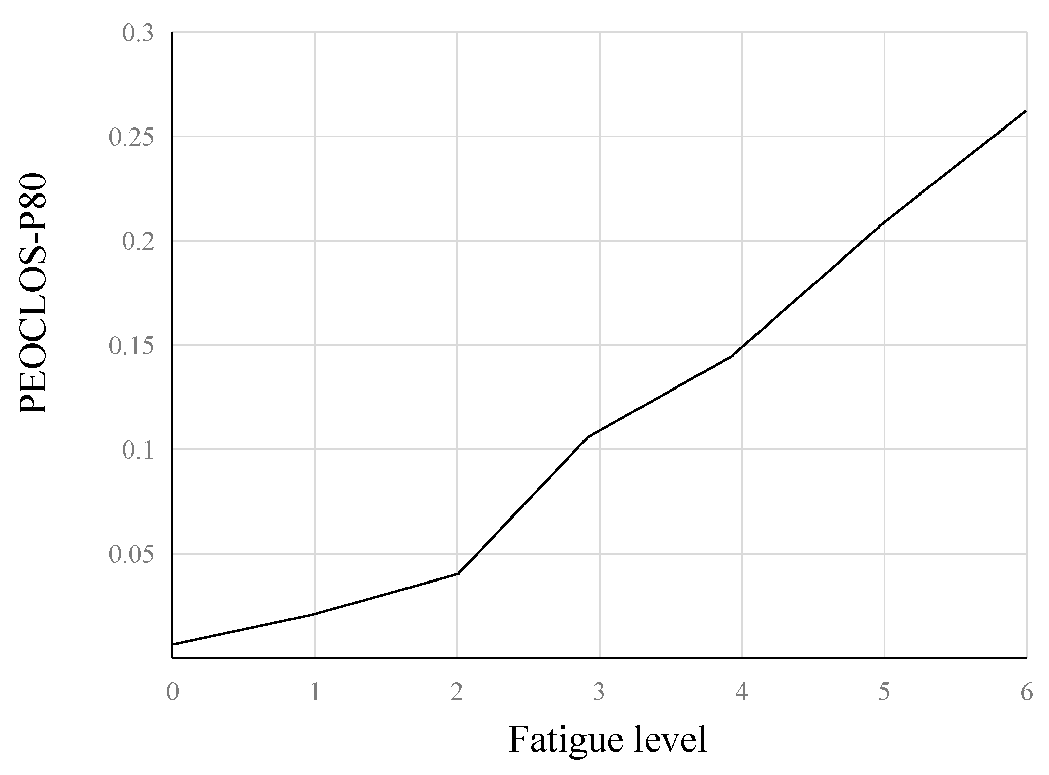
Figure 7 shows that the PERCLOS value (for P80) is positively correlated with the degree of fatigue. Therefore, we can take the PERCLOS value of controllers as the indicator of their eye fatigue, and quantitatively describe the fatigue state of controllers through PERCLOS (P80).

2.3. Decision-Level Fatigue-Information Fusion Based on the Entropy Weight Method

The concept of entropy is often used in information theory to characterize the degree of dispersion in a system. According to the theory behind the entropy weight method, a higher information–entropy index indicates data with a smaller degree of dispersion, and the smaller the impact of the index on the overall evaluation, the lower the weight [23]. According to this theory, the entropy weight method determines the weight according to the degree of discreteness in the data, and the calculation process is more objective. Therefore, the characteristics of information entropy are often used in comprehensive evaluations of multiple indicators to reasonably weight each indicator.

The main steps of the entropy weight method are as follows:

1. Normalization of indicators. Assuming that there are $n$ samples and $m$ indexes, $x_{ij}$ represents the value of the $j$th indicator ($j=1,2,\dots ,m$) corresponding to the $i$th sample ($i=1,2,\dots ,n$), then the normalized value ${x_{ij}}^{\mathrm{*}}$ can be expressed as

$${x_{ij}}^{*}=\frac{x_{ij}-x_{min}^j}{x_{max}^j-x_{min}^j}$$

(14)

where $x_{min}^j$ and $x_{max}^j$ represent the minimum and maximum values of the indicators, respectively.

2. Calculate the proportion of the $i$th sample value under index $j$:$p_{ij}=\frac{x_{ij}^{*}}{{\sum }_{i=1}^n{x}_{ij}^{*}}$.

3. Calculate the entropy of index $j$. According to the definition of information entropy, the information entropy of a set of data values is

$$E_j=-\mathit{ln} (n{)}^{-1}{\sum }_{i=1}^{n{\sum }_{ij}}{P}_{ij}ln$$

(15)

where, when $p_{ij}=0$, the information entropy is

$$\underset{p_{ij}\to 0}{lim}{p}_{ij}\mathit{ln} p_{ij}=0$$

(16)

4. Calculate the weight of each indicator.

$$W_j=\frac{1-E_j}{{\sum }_{j=1}^m(1-E_j)}$$

(17)

After obtaining the information entropy of each index, the weight of each index $W_j$ can be calculated using Formula (17).

3. Experiments and Verification

3.1. Data Acquisition Experiment

The experimental data were collected from the air traffic control simulation laboratory. We used the same type of simulator equipment as the Air Traffic Control Bureau at the experiment scenario, and invited six licensed tower controllers to participate in data collection with the cooperation of the Air Traffic Control Bureau.

Specifically, the radar control equipment in the experiment is shown in Figure 8. Key data acquisition equipment includes controller radio telephony recording equipment and facial data acquisition equipment. Speech data were collected directly from the radio telephony communication system, and eye-video data were collected using a camera with a resolution of 1280 × 720 at 30 fps. The participants included three male and three female certificated air traffic controllers from the Air Traffic Control Bureau. They are all from East China and have more than three years of controller work experience. All subjects were required to have adequate rest (>7 h) every night on rest days, and no food, alcohol, or drinks that might affect the experimental results. All experimental personnel were fully familiar with the control simulator system. All subjects were informed of the experiment’s content and had the right to stop the experiment at any time.

The experiment lasted for one week, and was designed according to the scheduling system in the actual control work. Severe fatigue is less common during the work process of air traffic controllers. We increased the workload appropriately to avoid a significant difference between the amount of data collected in the non-fatigued and fatigued states. During the week, the six controllers were conducted 24 h of experiment every day on Monday, Wednesday, Friday, and Sunday, and the controllers were prescribed to have complete rest on Tuesday, Thursday and Saturday, and they were required to sleep for more than seven hours. Each experimental day contained six periods of work and six periods of rest of two hours each. Each controller worked for two hours, rested for two hours, and completed the experiment for 24 h in turn. This experimental design was fully consistent with the characteristics of the actual controller post. On the experimental days, the first set of work experiments were conducted from 0:00 to 2:00 for each controller. After two hours of work, the first period of rest was started from 2:00 to 4:00. At the end of each period of work, each controller was asked to fill in the Karolinska Sleepiness Scale (KSS) [24], which took 10 min. They then rested for 110 min. After two hours of work, the controller is scheduled to rest for two hours, which is entirely consistent with the actual work schedule of the controller. The controlled work experiments alternated with rest periods, with up to 12 h of work and 12 h of rest periods within each working day.

KSS is a reliable fatigue detection scale, with scores ranging from one to ten reflecting the subject’s state from alert to almost unable to maintain clarity. According to the usual practice of KSS, when the questionnaire score is greater than or equal to seven, we determine that the controller is in a state of fatigue. At the end of the experiment, fatigue was determined according to the fatigue scale filled out by each controller, which was used as the label for the test data. After the experiment, we obtained a total of 462 min of valid voice data and 29 h of valid facial-video data.

3.2. Experiments on Speech-Fatigue Characteristics

We first combined traditional speech features including the MFCC, short-time-average zero-crossing rate, and maximum Lyapunov index, and verified the effectiveness of the FSVM using the classification accuracy of these features. We extracted the largest Lyapunov exponent ${\lambda }_{max}$ in the speech signal using data near-fitting and the characteristics of small-sample data. Figure 9 shows the fusion detection process for multiple speech features.

In order to obtain a clearer understanding of the classification performance of each classifier, we input relevant parameters, as presented in

Table 1. Internal classifier parameters.

Classification Algorithm	Penalty Parameter $\mathit{C}$	Kernel-Function Scaling Parameter $\mathit{\sigma }$	Number of Support Vectors
Standard SVM	64	0.0625	62
Improved FSVM	128	0.125	39

.

We selected 2010 speech data (for three males and three females) from the controller speech database as the training set (comprising 1030 fatigue samples and 980 normal samples) for target feature extraction and analysis. Data collected in the past has been processed as necessary and divided into short frames with a window function length of 25 ms. The step size between successive windows was set to 10 ms, and the number of filters used was 40. According to the feature extraction method, the 12th-order MFCC, short-time-average zero-crossing rate, and maximum Lyapunov exponent were extracted from the speech samples under fatigue and normal conditions. The extraction results were tested statistically to identify which of the above features differed significantly from the fatigue state; the results are presented in

Table 2. Differences in speech features between different states.

Phonetic Feature	Normal Sample	Fatigue Sample	t	Significance (p = sig)
Short-time-average zero-crossing rate (times/frame)	71.4 ± 6.2	66.9 ± 7.3	3.67	p = 0.041 < 0.05
12th-order MFCC	−0.91 ± 0.47	0.14 ± 0.51	7.62	p < 0.01
Maximum Lyapunov exponent	0.34 ± 0.07	0.25 ± 0.05	10.2	p < 0.01

.

We performed an Analysis of Variance (ANOVA) on three speech features. Our hypotheses are: (1) the short-time-average zero-crossing rate speech feature is related to the level of fatigue; (2) the 12th-order MFCC speech feature is related to the level of fatigue; (3) the maximum Lyapunov exponent speech feature is related to the level of fatigue. The mean ± standard deviation values are shown in Table 2.

In Table 2, the “Normal sample” represents the mean ± standard deviation of the speech features under normal conditions, while the “Fatigue sample” represents the mean ± standard deviation of the speech features under fatigue conditions. The “t” represents the t-test, which is the difference between the sample mean and the population mean. The significance level “p” represents the probability of the previous three hypotheses being true. Since the p-values in Table 2 are all less than 0.05, the three types of speech features have changed significantly under fatigue conditions. The significance level p-values of MFCC and maximum Lyapunov exponent are less than 0.01, so the differences in these two features before and after the controller’s fatigue can be considered to be significant, and these two features are particularly good at representing the fatigue state of the human body. Although the significance level p-value of the short-time average zero-crossing rate is slightly higher than that of MFCC and maximum Lyapunov exponent, its value is still less than 0.05, so this type of speech feature can also be used for fatigue detection.

In order to verify the usefulness of various speech features in detecting controller fatigue, we combined the features in different ways and used the standard SVM and the improved FSVM to classify and detect each combination. We use the data from the previous databases as the training data and the data collected in this experiment as the test data. The two types of speech data are strictly separate for classifiers. The test results after 50% cross-validation are presented in

Table 3. Test results for speech-fatigue characteristics.

Group	SVM Accuracy	FSVM Accuracy
MFCC + short-time-average zero-crossing rate	75.4%	77.1%
MFCC + maximum Lyapunov index	78.3%	79.5%
Short-time-average zero-crossing rate + maximum Lyapunov index	73.1%	73.8%
MFCC + short-time-average zero-crossing rate + maximum Lyapunov index	80.4%	82.5%

.

Table 3 indicates that the fatigue classification performance was worse for the short-time-average zero-crossing rate than for the other two features. Combining the three features produced the best classification performance, which was due to the traditional features and nonlinear features complementing each other. Moreover, the table indicates that the improved FSVM classifier had higher accuracy than the traditional SVM, which was due to the optimization of the membership determination method.

3.3. Experiments on Eye-Fatigue Characteristics

The OpenCV software library was used to detect eyes in the images. The human-eye-detection algorithm adopted in this study can accurately determine the eye area in both the open- and closed-eye states.

This study analyzed sub-images of the right eyes of the experimenters, and calculated the aspect ratio $\lambda$ of the eye by applying equalization, binarization, and other processing methods to the images. The calculation process of the length-width ratio of the eye is shown in Figure 10.Among the 3783 eye images extracted, 748 images had $\lambda$ values of <0.23, resulting in an eye PERCLOS value of 0.20 for experimenter 1 during this period.

In order to determine the fatigue value of controllers at different time periods more objectively, the Maximum Continuous Eye Closure Duration (MCECD) characteristic values of the experimenters during that time period were synchronously calculated according to the longest continuous eye-closure time within a single time period. As the degree of fatigue increases, the eyes become more difficult to open from a closed state, or more difficult to keep open when in an open state, leading to an increase in MCECD [25]. Considering that the radar signals used for air traffic control are updated every 4 s, we used a 40 s time window to detect the MCECD value of the controller during each time period, and included it in the calculation of the eye-fatigue value. We considered that a subject was in a state of fatigue when their eye-fatigue value was >0.3. Therefore, 0.3 is set as the threshold value. When MCECD is greater than 0.3, the subject is considered to be in a state of fatigue; when MCECD is less than or equal to 0.3, the subject is considered to be in a state of no fatigue. The fatigue state of the six air traffic controllers was judged using the threshold method, and the average value was taken. The accuracy of the discrimination results compared with the results of the KSS scale was shown in the following table. The corresponding accuracy values are listed in

Table 4. Eye-fatigue values calculated for experimenter 1.

Time Interval	MCECD (s)	Eye-Fatigue Value	Accuracy
0:00–2:00	0.48	0.34	83.2%
4:00–6:00	0.08	0.34	82.2%
8:00–10:00	0.82	0.33	79.5%
12:00–14:00	0.77	0.18	78.9%
16:00–18:00	0.97	0.23	88.1%
20:00–22:00	0.82	0.19	86.6%

.

The experimental results in Table 4 indicate that the average accuracy in identifying fatigue state based on eye characteristics was 83.08%. The experimental results show that the eye features have a high average accuracy in recognizing the fatigue characteristics of different controllers at different time periods, therefore, the eye fatigue features have good application values.

3.4. Multisource Information-Fusion Fatigue-Detection Experiment

The speech features were also evaluated numerically. By combining the trained decision model with $f(x)$, we applied sentence-by-sentence detection to the control speech data of each experimenter during each time period. This yielded the proportion of fatigued-speech epochs to the total number of speech epochs during the entire time period, which was used as the characteristic value for that experimenter’s fatigued speech during this time period. The speech-fatigue detection results are presented in

Table 5. Speech-fatigue detection results for experimenter 1.

Time Period	Total Number of Fatigued-Speech Epochs	Total Number of Speech Epochs	Fatigue Value
0:00–2:00	23	308	0.07
4:00–6:00	50	290	0.17
8:00–10:00	27	289	0.09
12:00–14:00	53	309	0.17
16:00–18:00	56	274	0.20
20:00–22:00	56	259	0.22

.

According to the theory of the entropy weight method, this study first assigned weights to the speech-fatigue value and eye-fatigue value at the decision level. We calculated the weights of the eye indicators and speech indicators of the six experimenters by normalizing the data and calculating the information entropy. The results are presented in

Table 6. Sample weights of the experimenters.

Experimenter	Eye Indicators	Speech Indicators
1	0.55	0.45
2	0.58	0.42
3	0.55	0.45
4	0.53	0.47
5	0.59	0.41
6	0.57	0.43

.

Based on the sample data from all experimenters, we averaged the weights of the indicators and used them as comprehensive indicator weights. The final indicator weights for the eye- and speech-fatigue values were 0.56 and 0.44, respectively. Based on the weights of the comprehensive indicators, we could obtain the comprehensive fatigue values of controllers at different time periods. We considered that a comprehensive fatigue value of >0.2 indicated a state of fatigue.

Table 7. Recognition accuracy of the comprehensive fatigue value.

Time Period	Comprehensive Fatigue Value	Accuracy
0:00–2:00	0.22	84.3%
4:00–6:00	0.25	85.2%
8:00–10:00	0.21	81.7%
12:00–14:00	0.18	89.6%
16:00–18:00	0.22	84.9%
20:00–22:00	0.20	90.3%

presents the comprehensive fatigue results for all experimenters.

The experimental results show that the recognition accuracy of the fatigue state based on integrated features was 86.0%, which was 2.2% and 3.5% higher than those for eye and speech features, respectively, indicating that fatigue recognition after fusion was more robust. In the experiment, some samples could not be correctly classified. The reason is that different controllers have different vocal characteristics and facial expression characteristics. It is undeniable that some people’s voice quality, timbre, and features such as eyes are similar to the performance of others when they are fatigued, which makes it difficult for the model to classify correctly. It can be seen that fatigue recognition still has great research potential.

4. Conclusions

This paper aims to solve the controller fatigue detection problem by first collecting linear and nonlinear radio telephony features. Then, the fused radio telephony features are classified and identified. Finally, the radio telephony recognition results and the eye fatigue feature recognition results are combined for decision-making to achieve a comprehensive assessment of the controller’s fatigue status.

The experimental results show that different speech feature combinations have different recognition accuracies, among which Mel Frequency Cepstral Coefficient + short-time-average zero-crossing rate + maximum Lyapunov index has the highest recognition accuracy. In the case of the fuzzy support vector machine classifier, the accuracy reached 82.5% compared to the evaluation results using the fatigue scale KSS. The accuracy in identifying fatigue state based on eye characteristics was 83.8%. For voice features and facial features, the initial fatigue results for the speech and eye feature layers were weighted using the entropy weight method, and finally comprehensive controller fatigue characteristic values were obtained through decision-level fusion. The accuracy of the fatigue detection method combined with eye and speech features was 86.0%, which was 2.2% and 3.5% higher than those for eye and speech features, respectively. The present research findings can provide theoretical guidance for air traffic management authorities to detect ATC fatigue. They might also be useful as a reference for controller scheduling improvement.

If the controllers’ clearances often need to be corrected, the controller may be fatigued. In the future, we hope to study the relationship between the number of corrections in the controller’s radiotelephony and the multiple levels of fatigue.