Abstract
The inlet is one of the most important components of a hypersonic vehicle. The design and optimization of the hypersonic inlet is of great significance to the research and development of hypersonic vehicles. In recent years, artificial intelligence techniques have been used to improve the efficiency of aerodynamic optimization. Deep generative models, such as variational autoencoder (VAE) and generative adversarial network (GAN), have been used in a variety of flow problems in the last two years, making fast reconstruction and prediction of the full flow field possible. In this study, a hybrid multilayer perceptron (MLP) combined with a VAE network is used to reconstruct and predict the flow field of a two-dimensional multiwedge hypersonic inlet. The obtained results show that the VAE network can reconstruct the overall flow structure of the hypersonic flow field with high accuracy. The reconstruction accuracy of complex flow structures, such as shockwaves, boundary layers, and separation bubbles, is satisfactory. The flow field prediction model based on the MLP-VAE hybrid model has a strong generalization and generation ability, achieving relatively accurate flow field prediction for inlets with geometric configurations outside the training set.
1. Introduction
The CFD solving process is usually time-consuming in a complex aerodynamic optimization problem. Consequently, various surrogate models are used to accelerate the flow field prediction process. Artificial intelligence (AI)-based surrogate models have become a research hotspot in recent years. AI and machine learning have an autonomy similar, in part, to human intelligence, constantly learning and improving the model. Its theoretical basis covers the disciplines of probability theory, mathematical statistics, and optimization theory. The model’s intrinsic parameters are continuously adjusted in the process of learning from the database to obtain the optimal prediction results. Commonly used machine learning surrogate models include the radial basis function (RBF), support vector machine (SVM), artificial neural network (ANN), etc. However, most of these surrogate models do not have sufficient ‘depth’ to characterize complex flow phenomena, and their limited characterization capability makes it difficult to predict the entire flow field [1].
In recent years, market applications such as image recognition, natural language processing, and autonomous driving have driven the development of artificial intelligence technologies. The resulting maturation of deep neural networks (DNNs) has expanded the characterization capabilities of artificial neural networks, enabling them to address more complex flow problems. Several studies on flow field prediction and aerodynamic optimization based on deep neural networks have emerged in recent years. Fujio et al. [2] implemented flow field prediction for axisymmetric hypersonic inlets based on a multilayer perceptron (MLP). The geometric parameters of the inlet and the node position are considered as the input, and the flow field parameters are the outputs. Brahmachary et al. [3] used proper orthogonal decomposition (POD) to downscale the dimension of the flow field and then reconstructed the flow field by a multilayer perceptron and moving least squares method. This improvement simplified the input information of the MLP network and facilitated the training of the MLP network, and the accuracy of its flow field prediction was significantly improved. POD has been a widely used method for flow field downscaling [4,5,6,7]. However, the reduced-order algorithm based on the POD method spreads the 2D flow field matrix into a 1D vector, which may cause the spatial relationship of the flow field to be lost. Yousif et al. [8] used generative adversarial networks (GAN) to reconstruct 3D flow fields from 2D measurements. GAN-based methods [9,10,11,12,13,14] show good ability for complex flow field reconstruction. Hu et al. [15] proposed RBF-GAN and RBFC-GAN to reconstruct flow fields, delivering better results than GANs. Autoencoders (AEs) and variational autoencoders (VAEs) based on convolutional neural networks can take full account of the spatial relationships of the flow field structure and the translational invariance of the physical laws of flows. Deng et al. [16] and Wang et al. [17] performed feature extraction and reconstruction of a supercritical airfoil flow field using AE and VAE, respectively. Wang et al. [17] also showed that the VAE has a higher accuracy in flow field reconstruction than the POD method. Dubois [18] used VAE to predict an unsteady flow field from limited measurements. In addition, VAE has also been used to reconstruct and predict flow fields in aircraft turbomachinery [19], vehicle aerodynamics [20,21], combustions [22,23] and supersonic combustors [24,25], which also achieved good accuracy.
This paper focuses on the hypersonic inlet, which is an important component of a supersonic combustion ramjet. Its main function is to provide an oxidant to the combustion chamber and to decelerate and pressurize the incoming flow to meet the requirements of combustion. The complex flow phenomena, such as shockwave, flow separation, and shockwave–boundary layer interaction in the hypersonic inlet, make the flow highly nonlinear, making the design and optimization of the inlet difficult. Due to the complexity of the flow, a slight change in the geometric parameters can make a large difference in the performance of the inlet. Convolutional neural network technology is used in this paper to achieve rapid prediction of the flow field of hypersonic inlets and optimize the hypersonic inlet. First, five hundred two-dimensional (2D) three-wedge inlets are randomly sampled, with the wedge angles as the design parameters; second, the inlet samples are calculated with the help of a CFD solver to obtain the flow field dataset; then, a VAE model is built to learn the abovementioned dataset to realize the feature extraction and reconstruction of the flow fields, and a MLP network is trained to learn the relationship between the design parameters and the flow field features extracted by the VAE model so that a surrogate model is obtained that can predict the flow field according to the design parameters.
2. Validation of the CFD Method
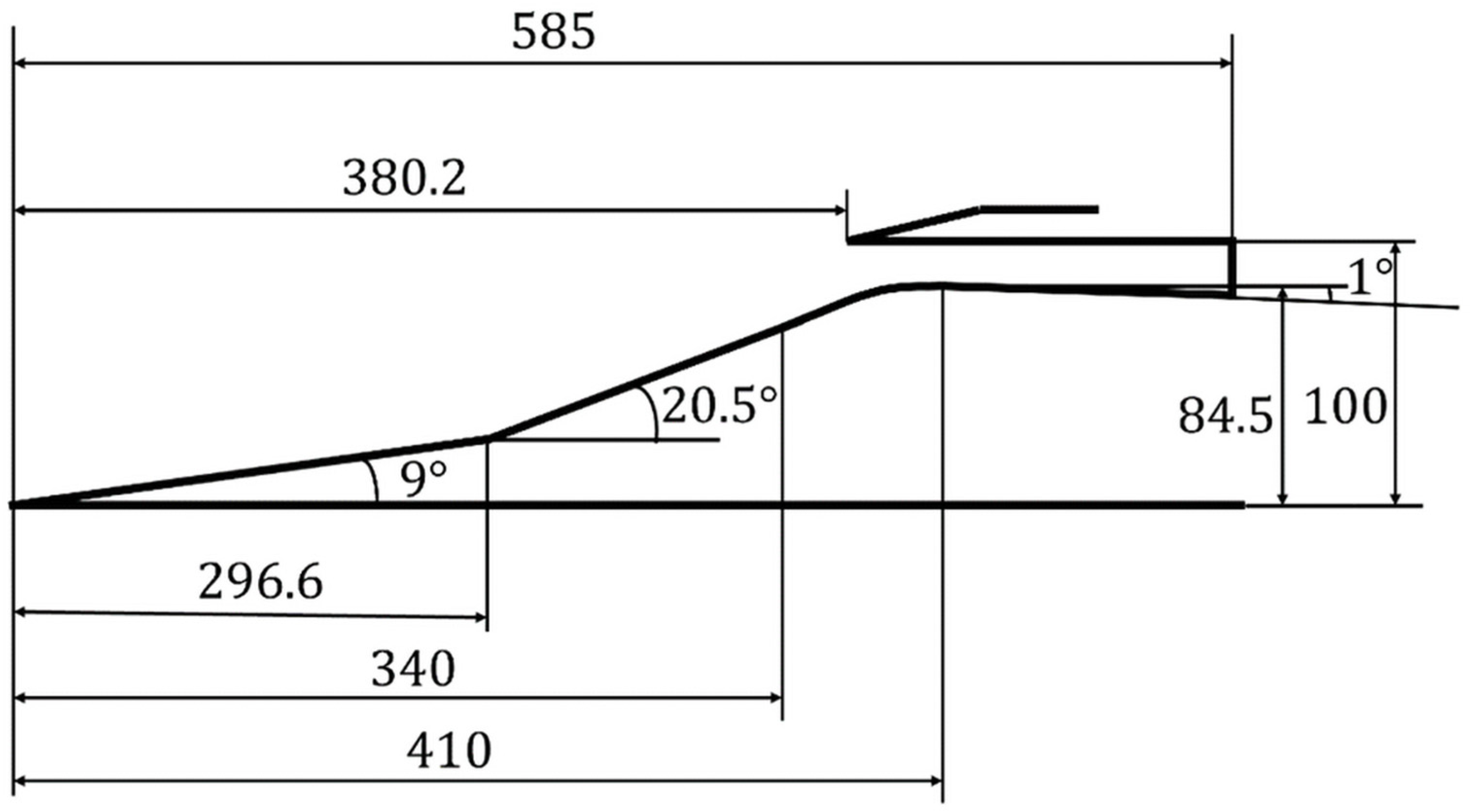
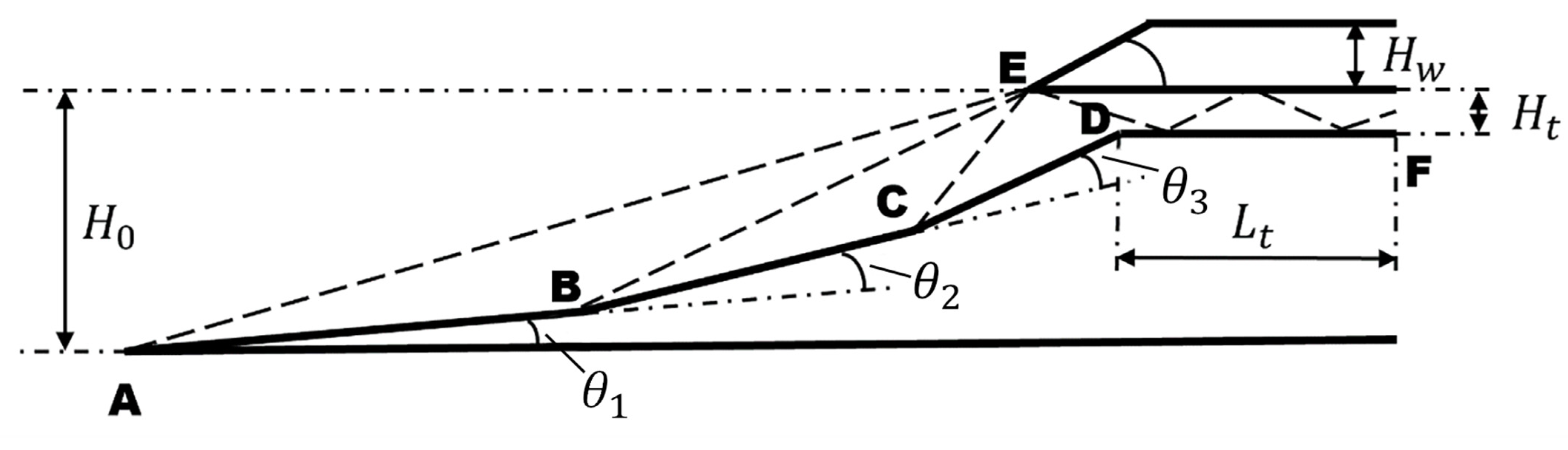
The flow field of a 2D inlet is considered in this study. A test case with experimental data, which is the GK-01 inlet, is computed to test the accuracy of the CFD solver. The obtained results are compared with the experimental data in Ref. [26]. The geometric configuration of the GK-01 inlet is shown in Figure 1. The incoming flow conditions are kept consistent with the experimental conditions in Ref. [26], as listed in Table 1.

Figure 1.
Geometric configuration of the GK-01 inlet (unit: mm).

Table 1.
Incoming flow conditions for the GK-01 test case.
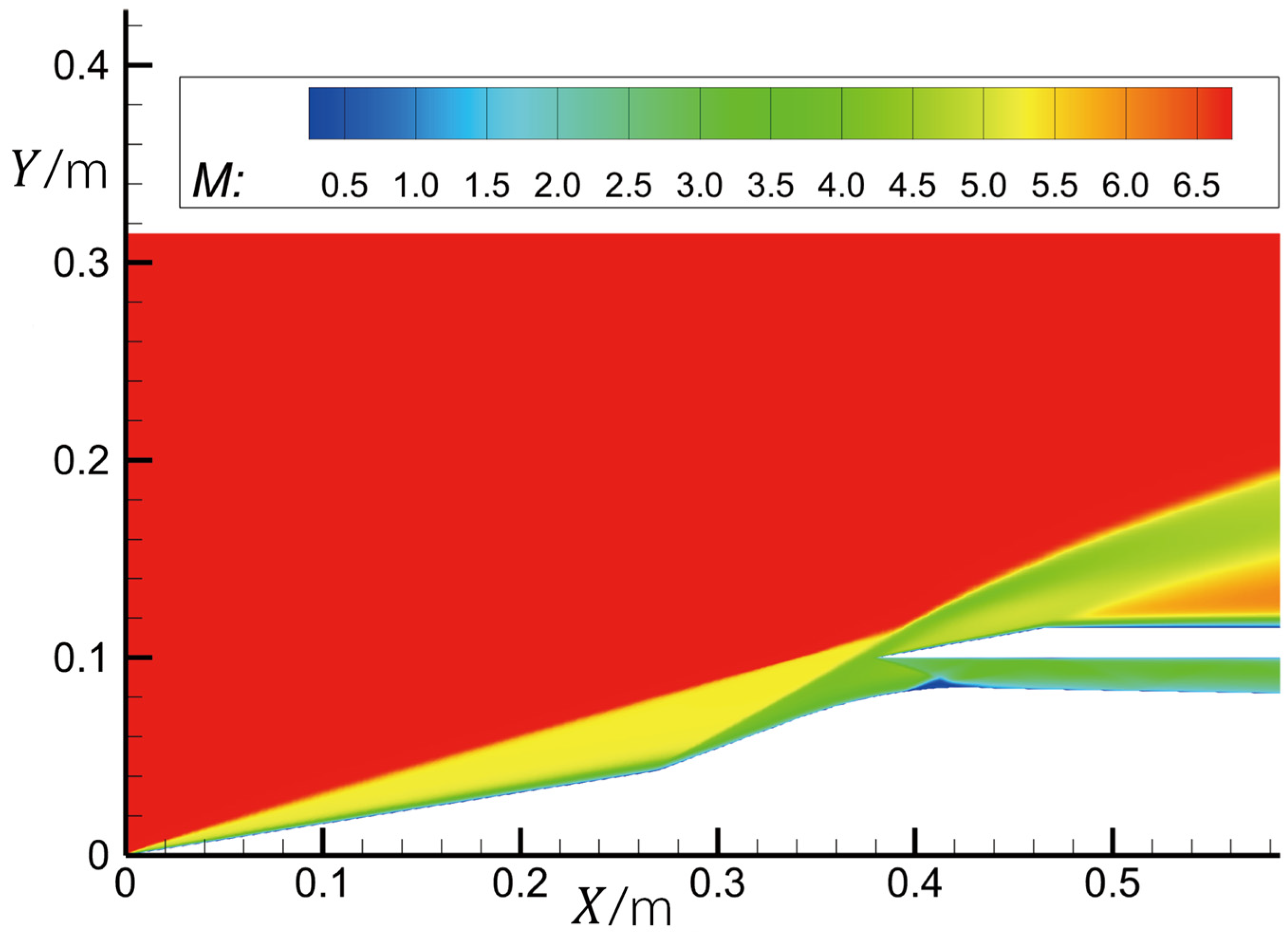
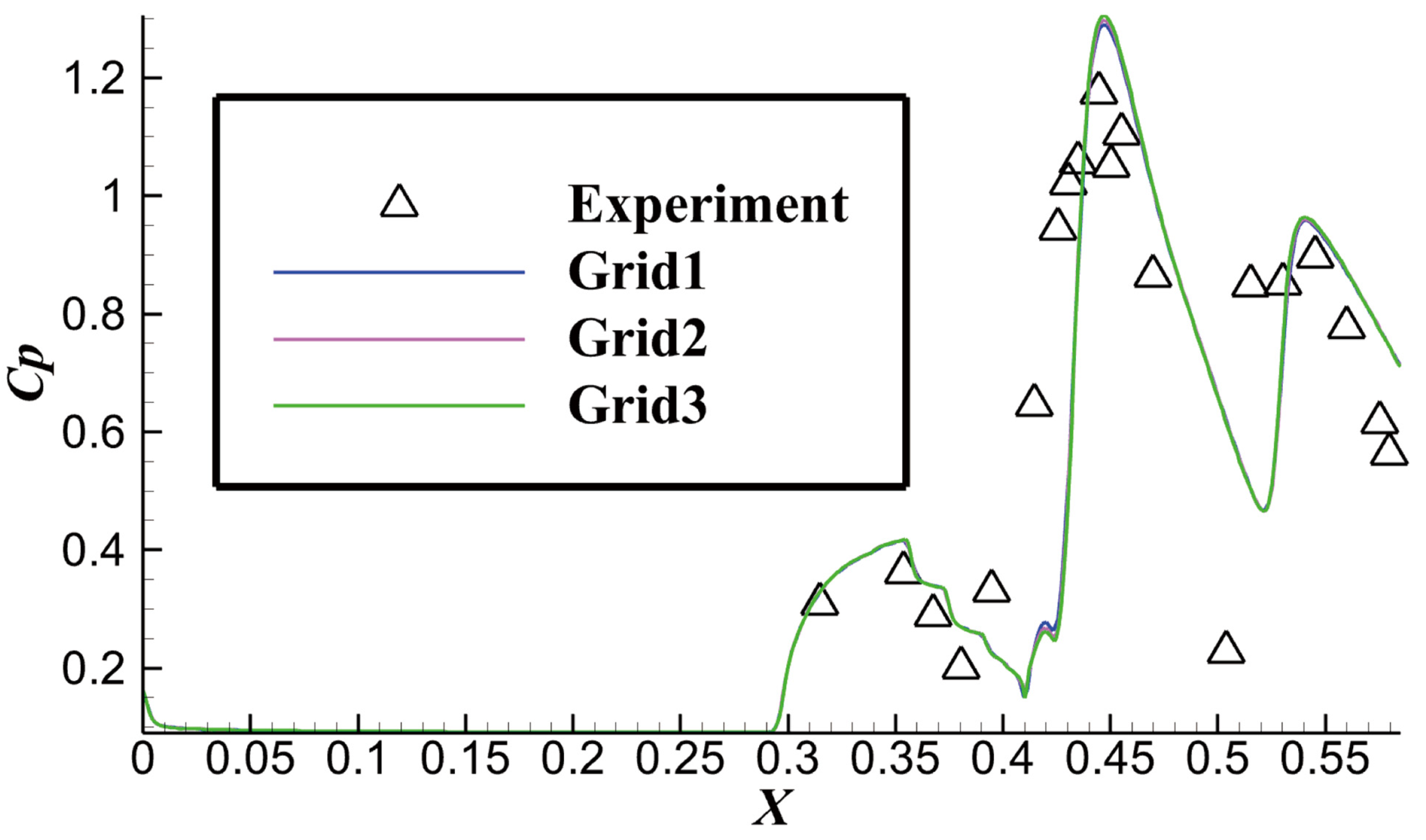
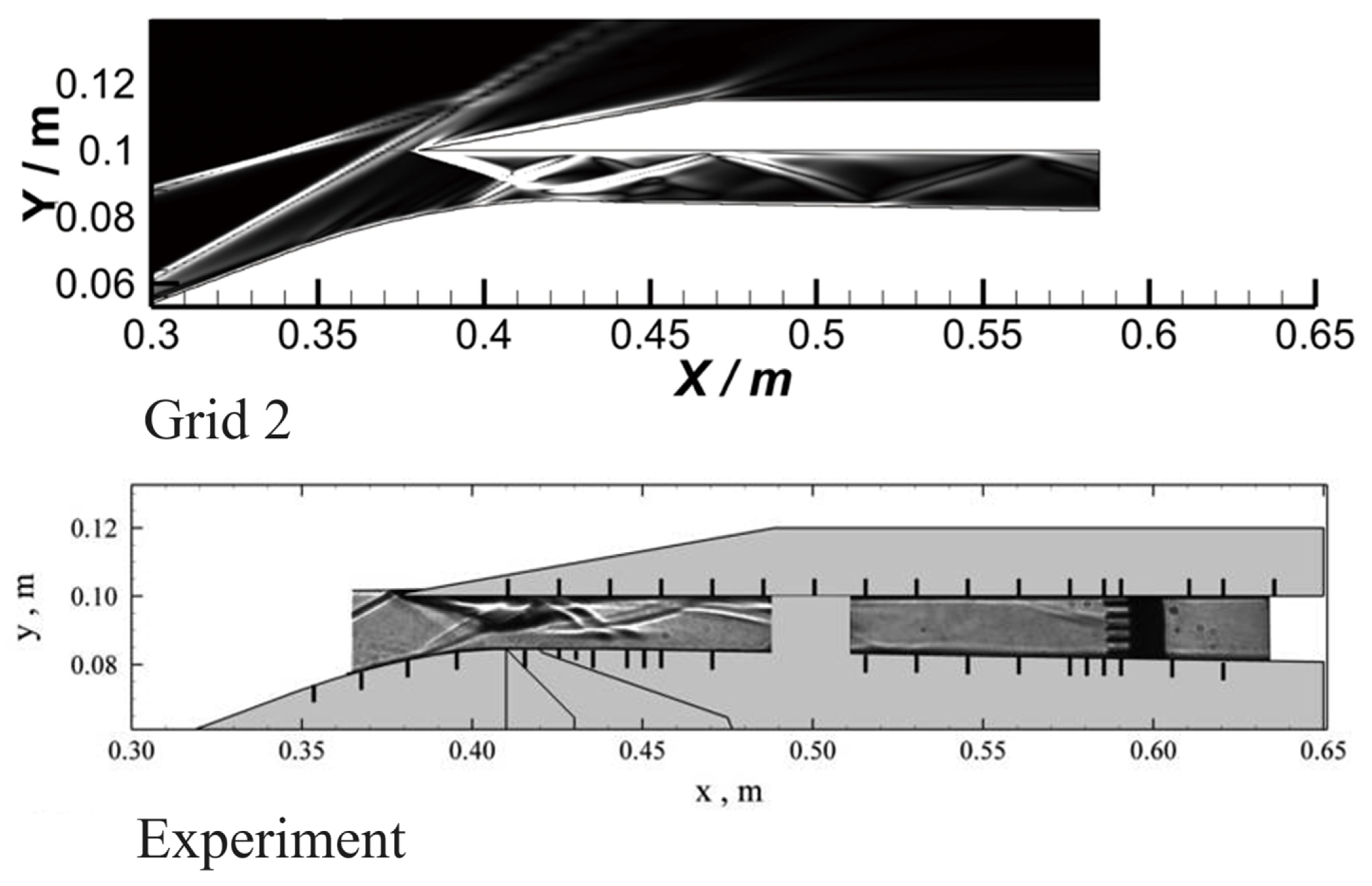
Figure 2 shows the Mach contour of the GK-01 inlet calculated by an unstructured CFD solver. The three shockwaves interfered near the inlet lip. There is a small flow separation near the inlet throat. A comparison of the calculated and experimental values of the pressure coefficient on the compression surface is shown in Figure 3. The fluid field is calculated with three different grid densities to test the grid convergence of the CFD computation in this study. Grid 1 represents a coarse grid, which has grid cells. Grid 2 is a medium grid and has grid cells. Grid 3 is a fine grid and has grid cells. The CFD results are in general agreement with the experimental results. The obtained results are also similar for the different grid densities, indicating good grid convergence. A grid density similar to the medium grid is applied in the following computation. Figure 4 shows the shockwave structures of the inlet, both CFD for Grid 2 and the experiment. It shows that the middle grid captures most of the shockwave structures in the hypersonic inlet.

Figure 2.
Mach number contour of the GK-01 inlet model.
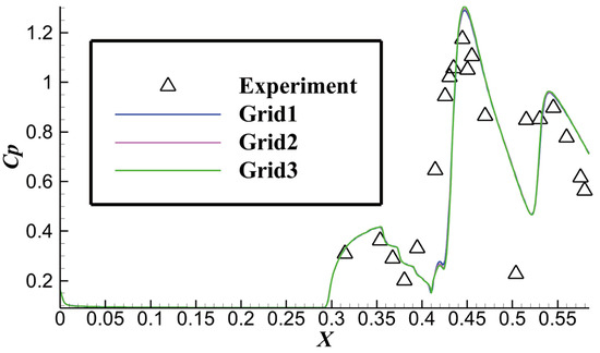
Figure 3.
Pressure coefficient on the compression surface of GK-01.
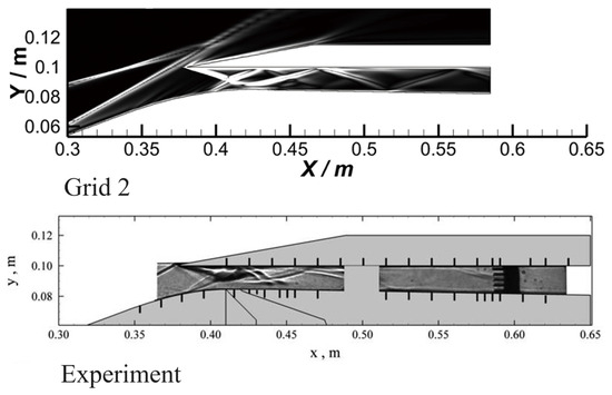
Figure 4.
Shockwave in the inlet [26].
3. Generation of the Flow Field Dataset
In this study, the flow field reconstruction of a 2D three-wedge hypersonic inlet is performed. The geometry of the inlet is shown in Figure 5. The entire inlet is integrated into the aircraft forebody, and the three wedge segments allow the incoming flow to be gradually deflected and compressed before entering the combustion chamber through the throat.
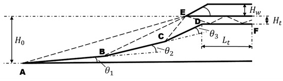
Figure 5.
Geometric configuration of a two-dimensional three-wedge hypersonic inlet.
To improve the efficiency of machine learning, the geometric configurations of the inlets in the dataset are predesigned and filtered based on shockwave equations. The shockwaves from the compression side (Points A, B, and C) are expected to converge at the inlet lip, Point E, to avoid leakage of the captured flow. We conduct the following design steps in the sampling process to achieve this requirement: (1) fix the inlet height and the throat height and then conduct independent uniform random samplings for the three wedge angles , and and (2) compute the length of each wedge segment through the shockwave equation and geometric relation to ensure that the oblique shockwaves converge exactly at the lip. The aspect ratio of isolators is fixed to 8, and and are also fixed. In addition, the total deflection angle ( + + ) of the airflow ranges from 18° to 26°, and the Mach number Ma5 of the airflow entering the throat ranges from 1.8 to 2.4. The incoming flow Mach number and the flight altitude .
The relation between the oblique shock angle and the deflection angle of the flow is shown in Equation (1), where is the deflection angle of the flow and is the Mach number before the shockwave. Solving Equation (1) yields two solutions, the smaller of which is the oblique shock angle.
The relation between the Mach numbers before and after the shockwave is shown in Equation (2), where the pre-wave parameters are subscripted as 1 and the post-wave parameters are subscripted as 2.
The values or ranges of the design parameters of the inlet in the dataset are listed in Table 2. The sample size is 500.
Table 2.
Values or ranges of the design parameters of the inlets in the dataset.
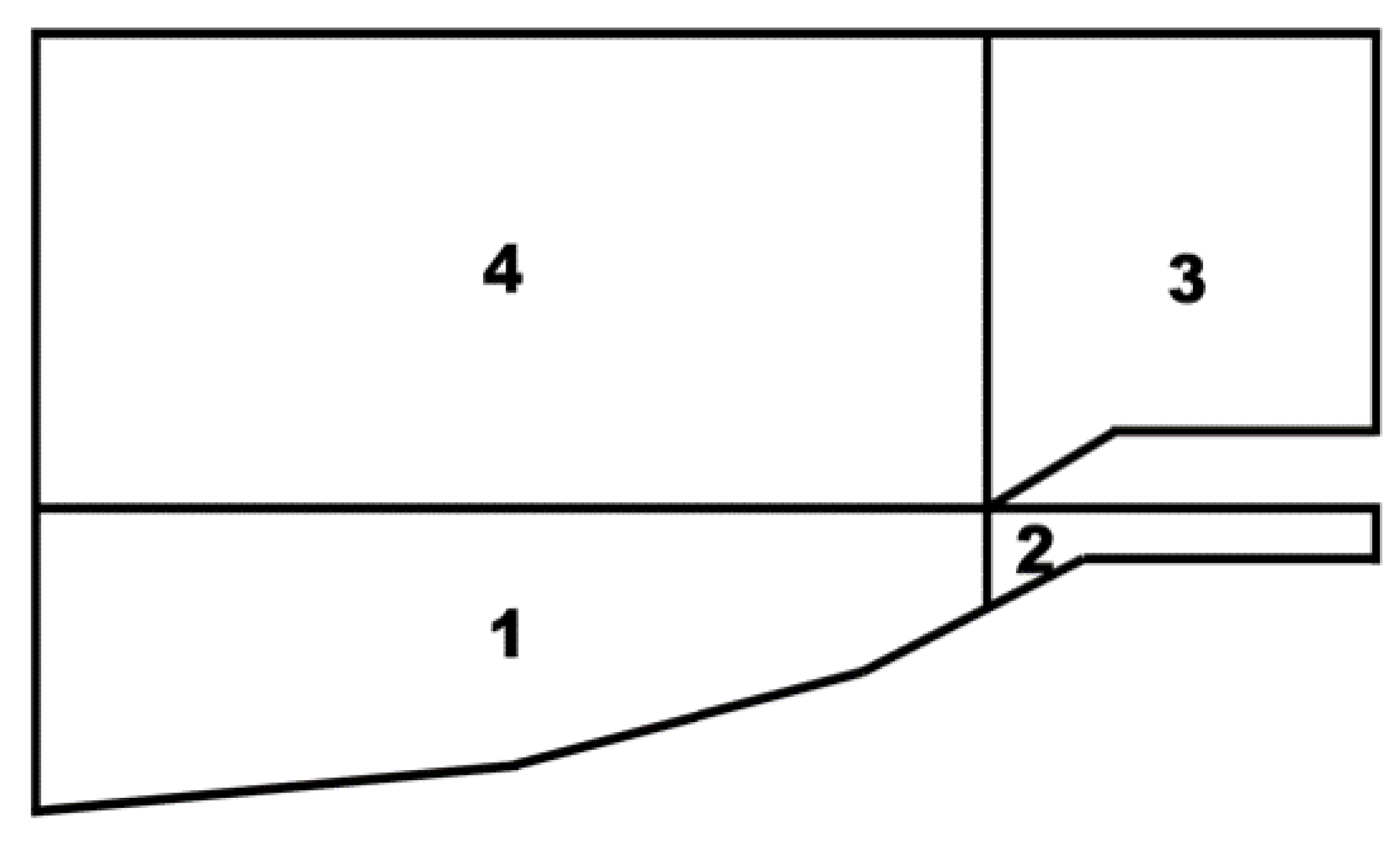
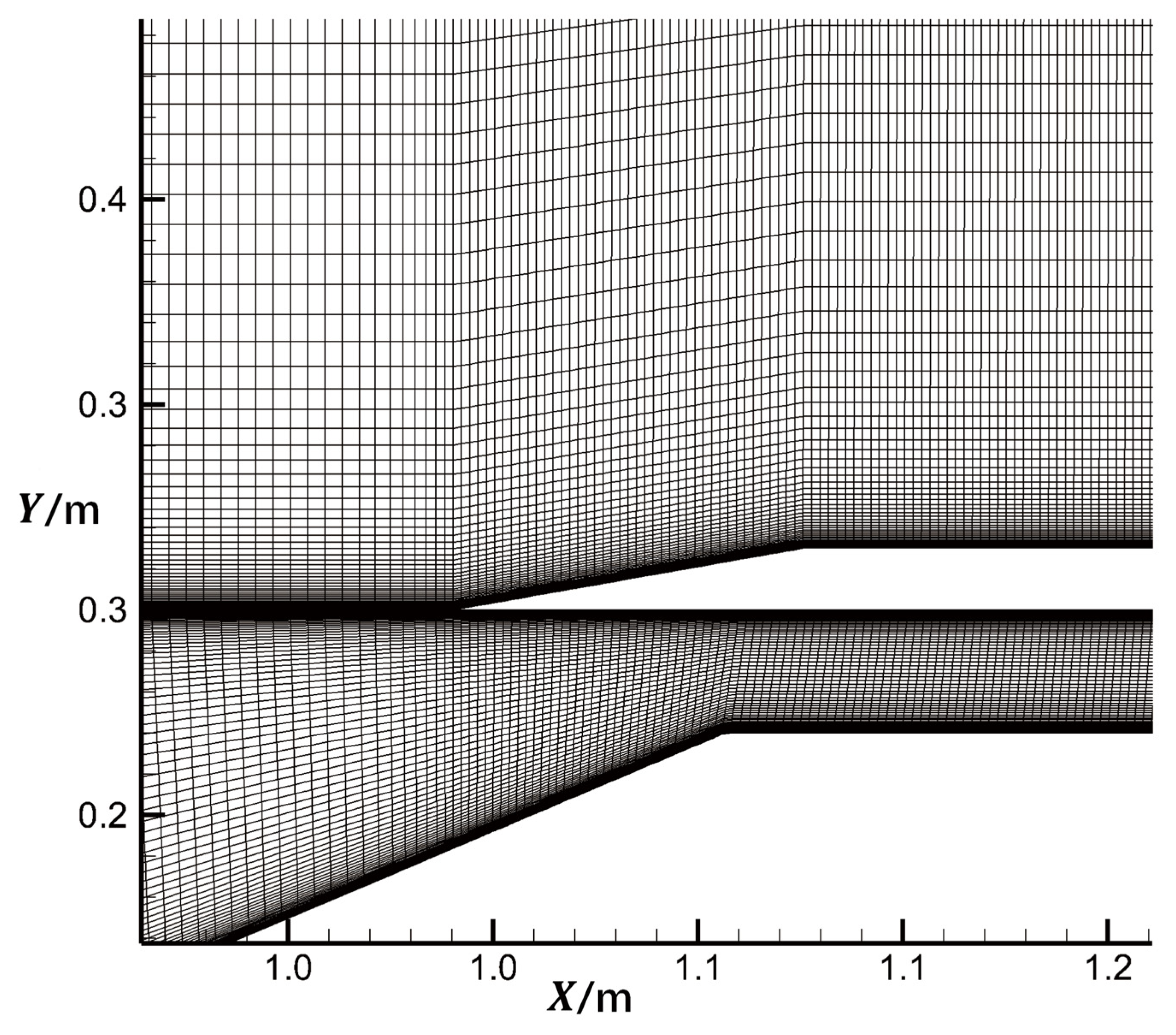
After the sampling process, the flow fields of the samples in the dataset are computed by the CFD solver. The grid block partition is shown in Figure 6. The entire inlet flow field is divided into four grid blocks according to geometry. The grid points of the four blocks are 250 × 100, 150 × 100, 150 × 120, and 250 × 120. Figure 7 shows the grid detail around the inlet lip. The grid is appropriately refined in the boundary layer.

Figure 6.
Grid block partition of the inlet.
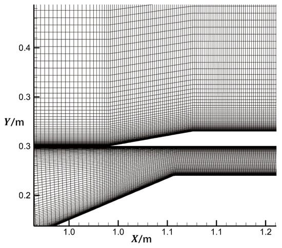
Figure 7.
Grid detail around the inlet lip.
The compressible Navier-Stokes equations coupled with the k-ε turbulence model are solved in the CFD solver. The wall condition is set to the nonslip condition with an isothermal value of 300 K. The initial conditions are the same as the incoming flow conditions. The calculation is terminated if the residual is less than or the iteration is more than 2000 steps. After the CFD computation, the velocities and , the temperature , and the static pressure are used for flow field reconstruction training and testing.
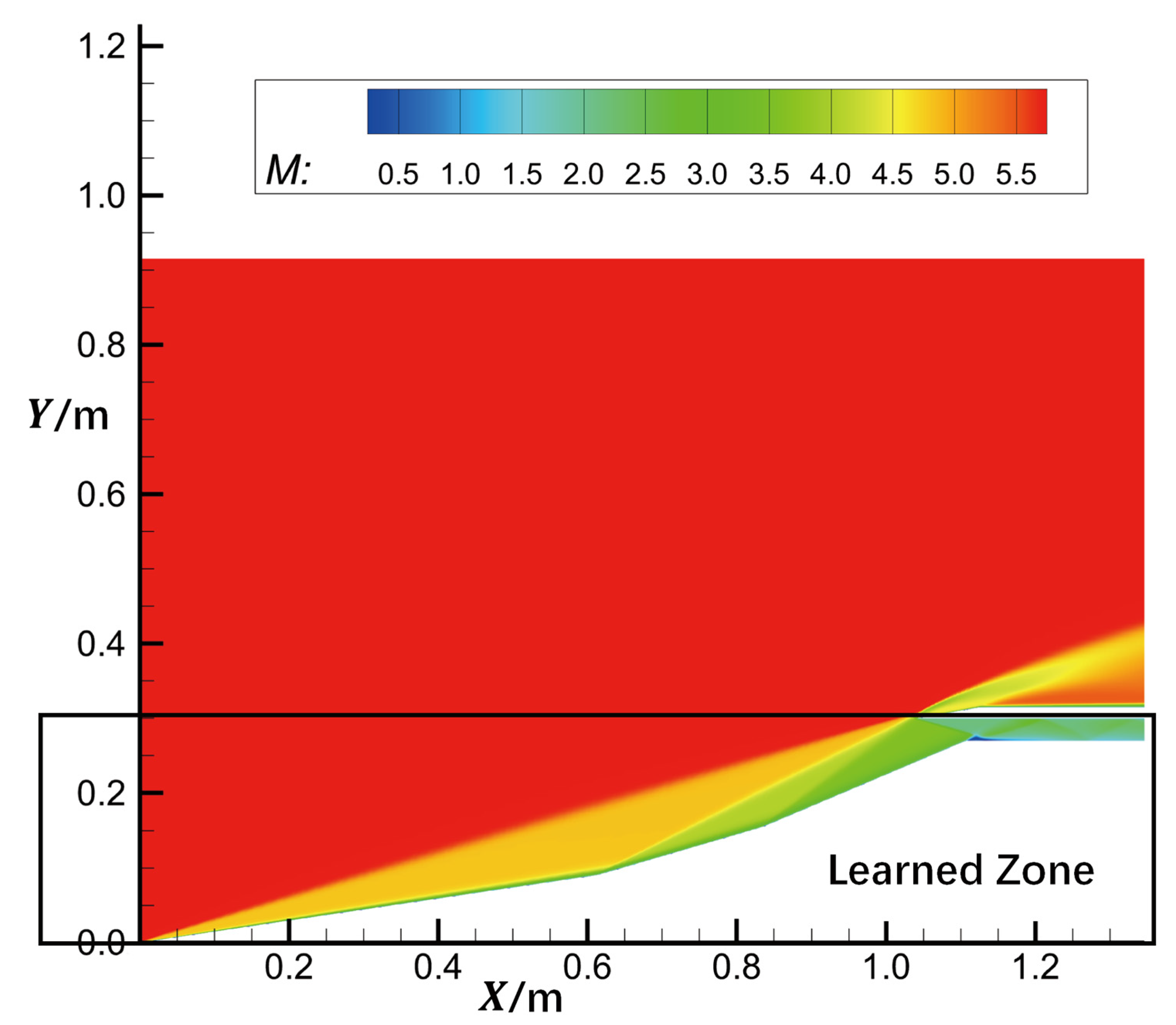
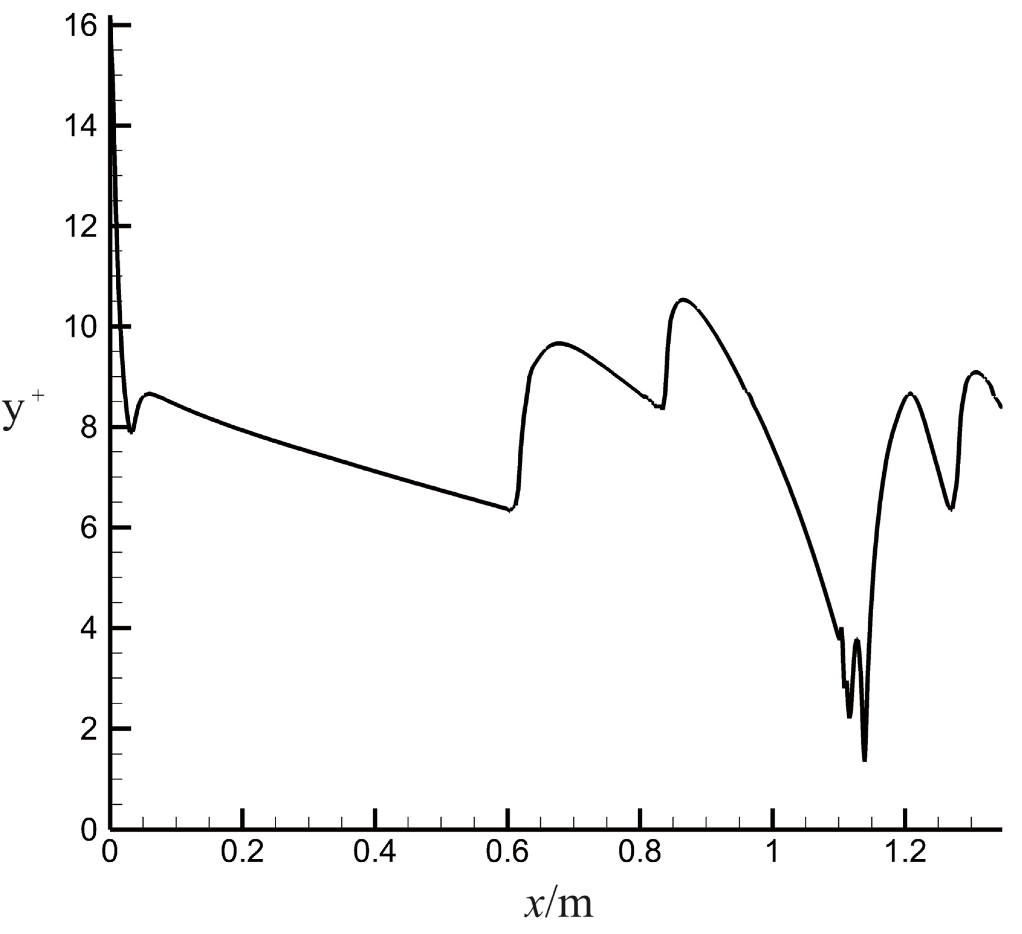
The incoming flow conditions for the dataset computation are listed in Table 3. We chose to train the model with incoming Ma 6 for engineering needs. The CFD method has been verified by a comparison with the experimental data of the GK-01 model with incoming Ma 7. Although the Mach numbers are different, the results may still be reliable enough, as done in Ref. [27]. Figure 8 shows the flow field of sample ID-001. Figure 9 shows the y+ value on the compression surface of sample ID-001. Since the k-ε model is adopted in this paper with a wall function, the y+ value is passable for our calculations. A black box is marked in the figure, which is the flow field zone used for machine learning training and testing. The VAE method proposed in this paper can be applied on any part of the flow field, while we only consider the flow captured by the inlet to improve the training efficiency. A total of 399 × 100 grid points are used for training.
Table 3.
Incoming flow conditions for the dataset.

Figure 8.
Flow field (Mach contour) of sample ID-001.

Figure 9.
y+ value on the compression surface of sample ID-001.
4. Structures of the Flow Field Reconstruction and Prediction Models
A flow field reconstruction and prediction model based on the VAE-MLP hybrid model is introduced in this section. We first compress and reconstruct the data of the 2D hypersonic inlet flow field based on a variational autoencoder (VAE) model. The trained VAE encoder is used for flow field data reduction and feature extraction; thus, the complex flow field data are compressed into a latent code vector in the eigenspace to characterize the flow field. The trained VAE decoder is also a flow field generator, which can recover a vector in the flow field eigenspace into a complete flow field. The VAE decoder is then combined with a multilayer perceptron (MLP) to achieve rapid prediction of the inlet flow field.
4.1. VAE Model
The VAE was originally proposed by Kingma et al. [28]. In this paper, the VAE model is built with reference to the method in [17], i.e., the residual blocks are used to build the encoder and decoder to increase the depth of the neural network and, thus, enhance the feature extraction capability of the VAE.
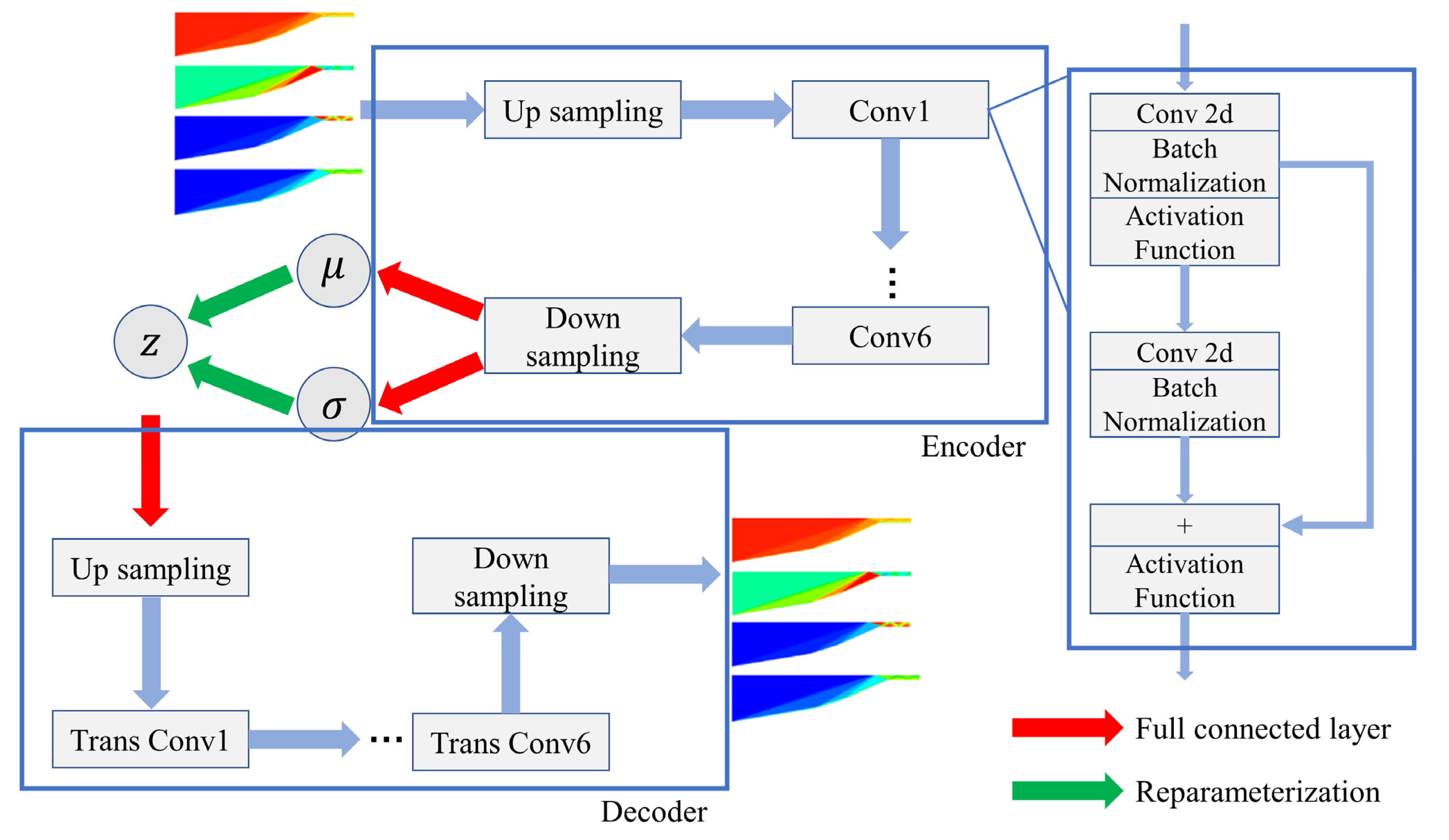
The structure of the VAE model in this paper is shown in Figure 10. In VAE, the encoder maps the input into a normal distribution.
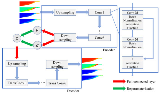
Figure 10.
A diagram of the VAE model.
A random sample from this distribution is taken to obtain the code for the data before decoding, which is called reparameterization.
where , and . Finally, the decoder maps into as the reconstructed result of .
in Equation (3) and in Equation (5) represent the parameters of the network to be trained, which are continuously optimized during the training process to improve the model performance. The loss function of the VAE model is shown below.
The loss function of VAE contains two components: namely, the K-L divergence and MSE loss. The β in Equation (6) adjusts the ratio of the K-L divergence and MSE loss. The larger , the stronger the VAE is in terms of feature decoupling and generating new samples; the smaller , the greater the VAE focuses on the reconstruction accuracy of the training samples; and when , the VAE is reduced to a general automatic encoder.
The detailed structure of the VAE model built in this paper is listed in Table 4. A convolution or transposed convolution residual block that contains a short-circuit operation is used as the basic structure to build the encoder and decoder, thus improving the depth and feature extraction capability of the network.
Table 4.
Detailed structure of the VAE model in this paper (FC: fully connected layer, Conv: convolution residual block, Trans conv: transposed convolution residual block, and N: dimensions of latent code vector).
4.2. MLP Model
After training the VAE model, we use a multilayer perceptron (MLP) to learn the mapping relationship between the inlet geometry parameters and the flow field feature parameters. However, the flow feature parameters are probabilistic distribution parameters rather than exact values. Therefore, when training the MLP model for flow field prediction, the mean value , i.e., the probability maximum position of the distribution , is used. After the training is completed, the trained MLP model is combined with the VAE decoder to obtain a flow field prediction model based on the three wedge angles.
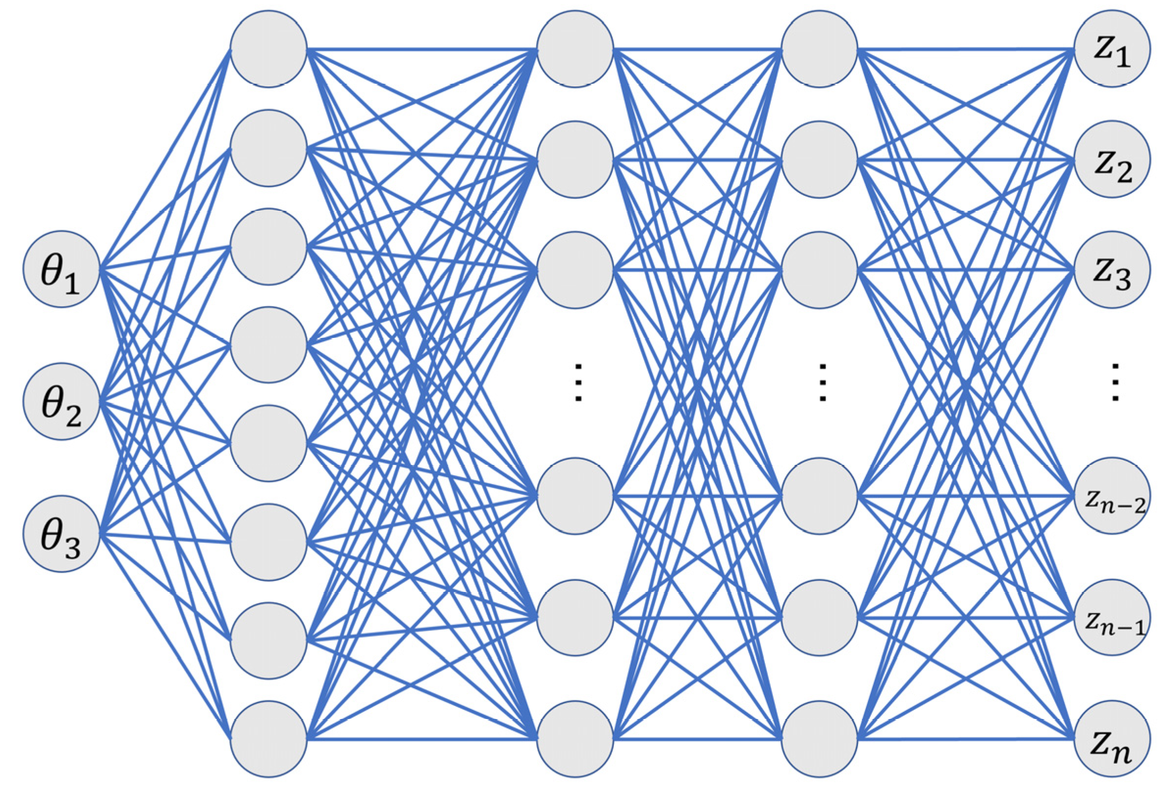
In this study, the number of neurons in the input layer is three, corresponding to the three wedge angles, and the number of neurons in the output layer is the same as the dimension of the VAE coding features. Three hidden layers of 8, 32, and 32 neurons are adopted in the MLP model. The structure of the MLP network is shown in Figure 11. MSE_LOSS is used as the loss function of the MLP model, and its expression is shown in Equation (7).
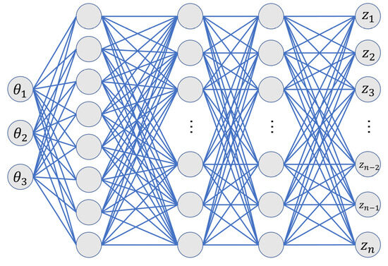
Figure 11.
The structure of the MLP network.
4.3. VAE-MLP Hybrid Model
Although the VAE enables the reconstruction of the flow field, obtaining the flow field of the inlet directly from the given geometrical parameters is expected in the design process, i.e., the three wedge angles. Therefore, we need to connect the decoder of the VAE to the MLP network to obtain the MLP-VAE hybrid model. The structure of the hybrid model is shown in Figure 12.
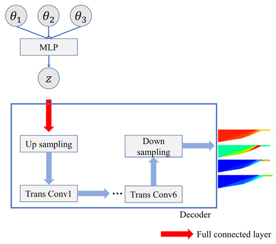
Figure 12.
Structure of the VAE-MLP hybrid model.
5. Results of the Model Training
In this paper, the training set includes 450 samples, while the testing set includes 50 samples. This section presents the training results of the model built in Section 4. First, several evaluation indicators used in the training process are provided. Then, the training results of the VAE model, the MLP model, and, finally, the MLP-VAE hybrid network are presented.
5.1. Evaluation Indicators of the Training
Before tuning the hyperparameters and other settings of the models, several indicators are defined to evaluate the quality of the flow field reconstruction or prediction. The following three indicators are adopted in this paper:
(1) Mean absolute error (MAE)
where is the number of flow field nodes; denotes the flow field quantities, i.e., , , and calculated by CFD; and is the flow field reconstructed or predicted by the machine learning model.
(2) Correlation coefficient
Because the absolute error is not intuitive to measure the relative error, in addition to the MAE, the correlation coefficient is used to evaluate the similarity of the flow field calculated by CFD compared with the reconstructed and predicted flow fields.
(3) Relative error of the total pressure recovery ( Error)
The total pressure of a compressible flow is
is the static pressure, is the specific heat ratio, and is the Mach number. The total pressure recovery is an important parameter of the inlet performance and is defined as follows:
The numerator is the average total pressure at the outlet, and the denominator is the total pressure of the incoming flow.
Finally, the relative error of the total pressure recovery is defined as follows:
where is the total pressure recovery of the reconstructed or predicted flow field, and σ is the total pressure recovery of the flow field calculated by the CFD solver.
5.2. Model Tuning
The composition and hyperparameters of the model do not change during the learning process, and they need to be tuned manually. In this paper, we sequentially tune the activation function, Adam optimizer’s , batch size, dimension of the latent code vector, and in the loss function and select the best parameters based on the training results. Due to limited space, the specific tuning process is not given in this paper; only the final settings of the model are marked in bold in Table 5.
Table 5.
Model tuning and the final settings of the model (marked in bold).
5.3. Results of Fluid Field Reconstruction Based on the VAE
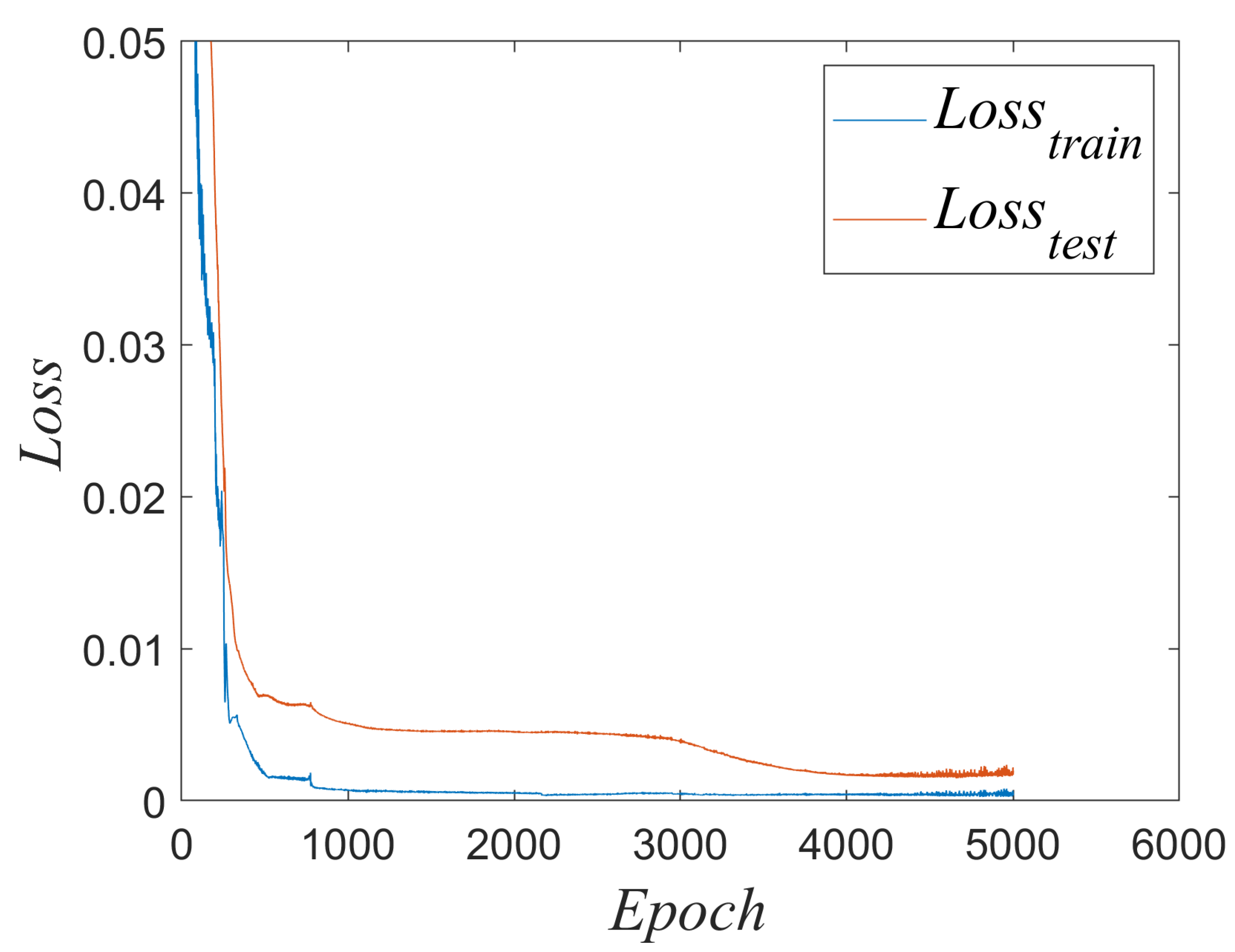
The VAE model was trained for 5000 epochs. The learning rate decay strategy is referenced in [17]. The initial learning rate is set to 0.0004, and the learning rate is reduced by half after every 1000 epochs. The decay curve of the loss function of the VAE model is shown in Figure 13. The final accuracy of the flow field reconstruction based on the VAE model is listed in Table 6. The values before the plus or minus sign in each cell are the mean values of the individuals in the dataset, and the values after the plus or minus sign are their statistical standard deviation. In the whole dataset, ranges from to , ranges from to , ranges from to , and ranges from to .
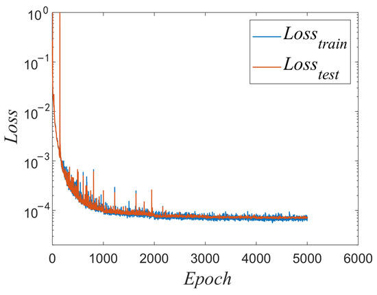
Figure 13.
Loss function of the VAE model.
Table 6.
Accuracy of the flow field reconstruction based on the VAE model.
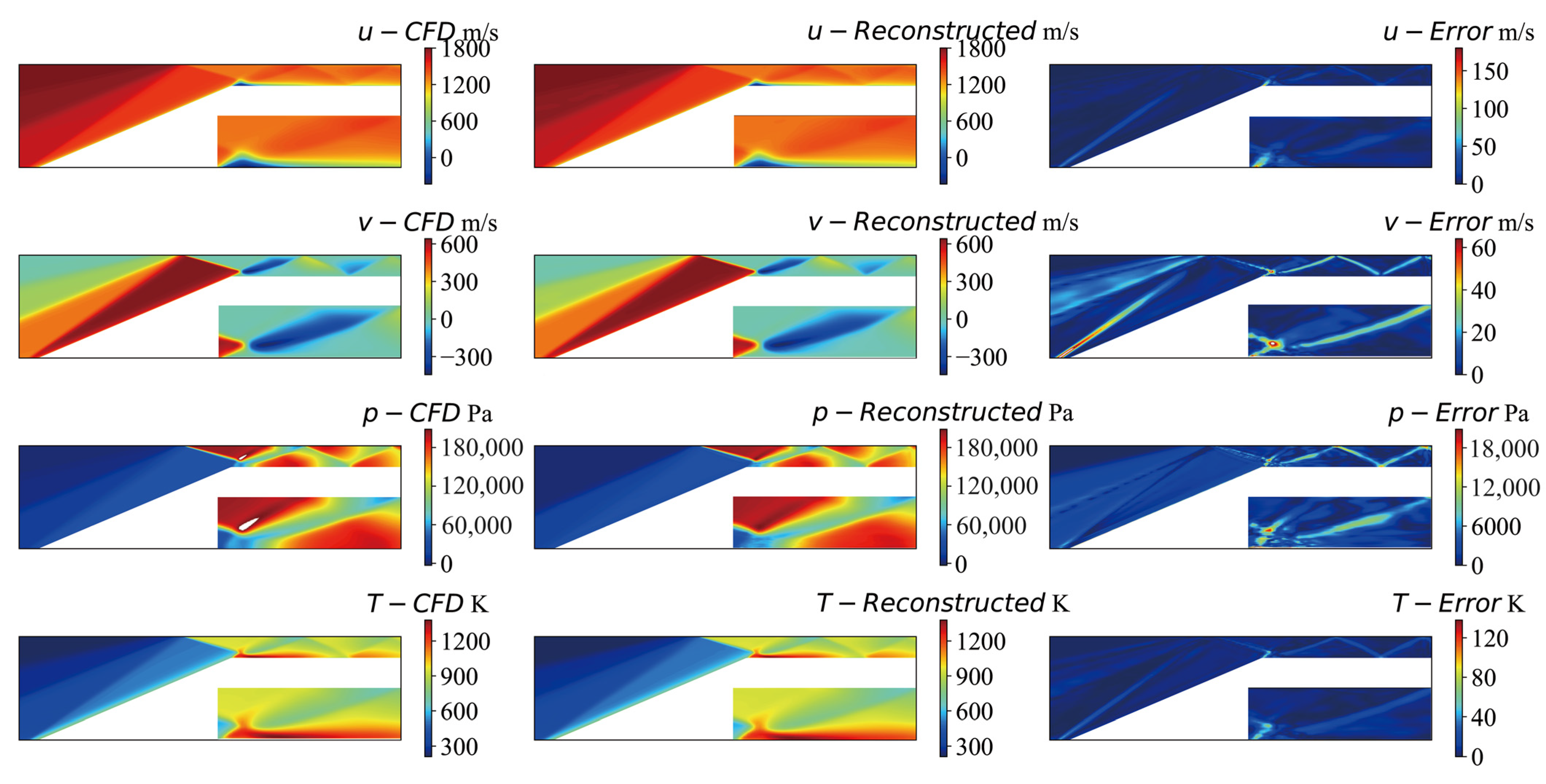
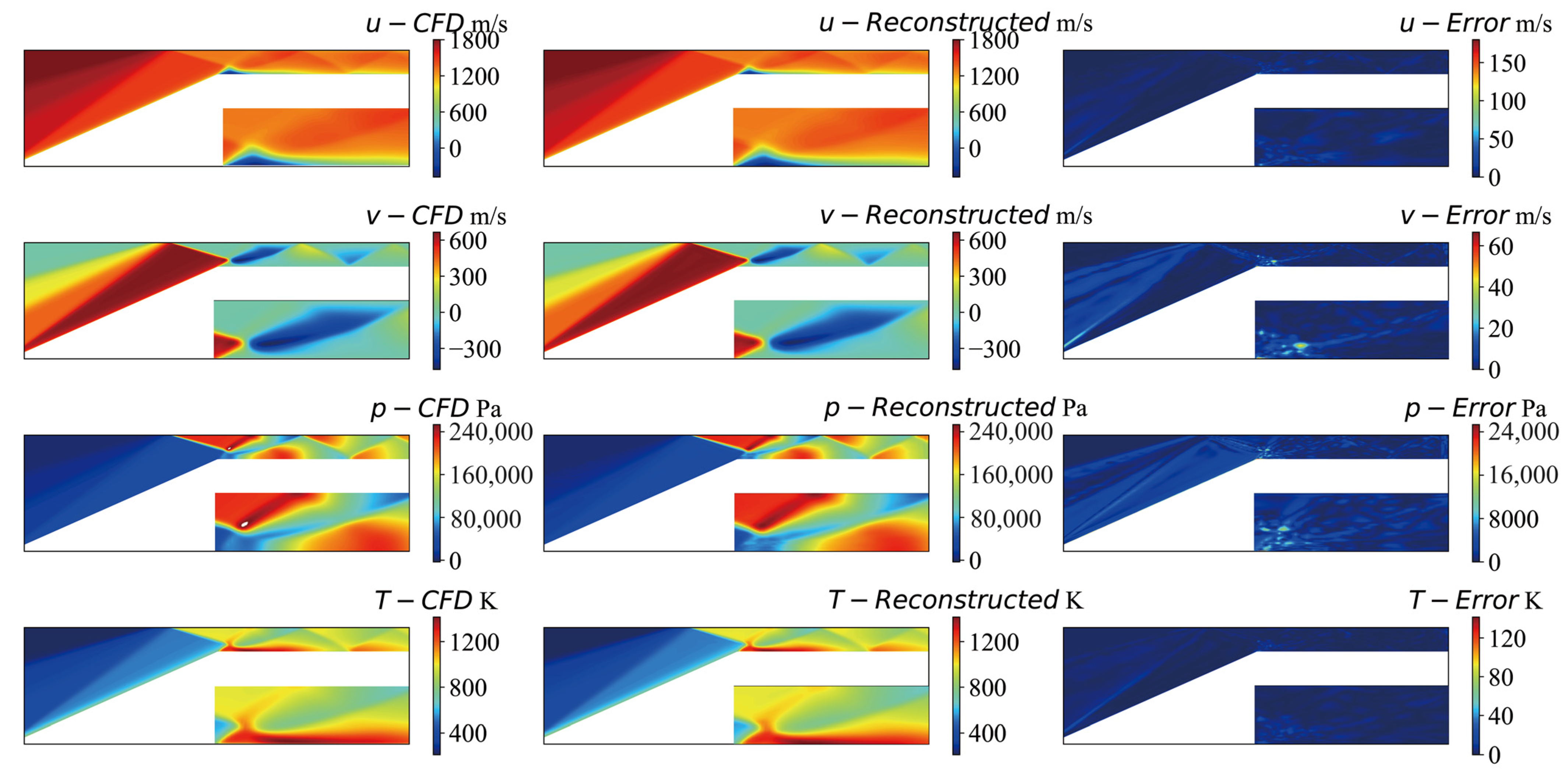
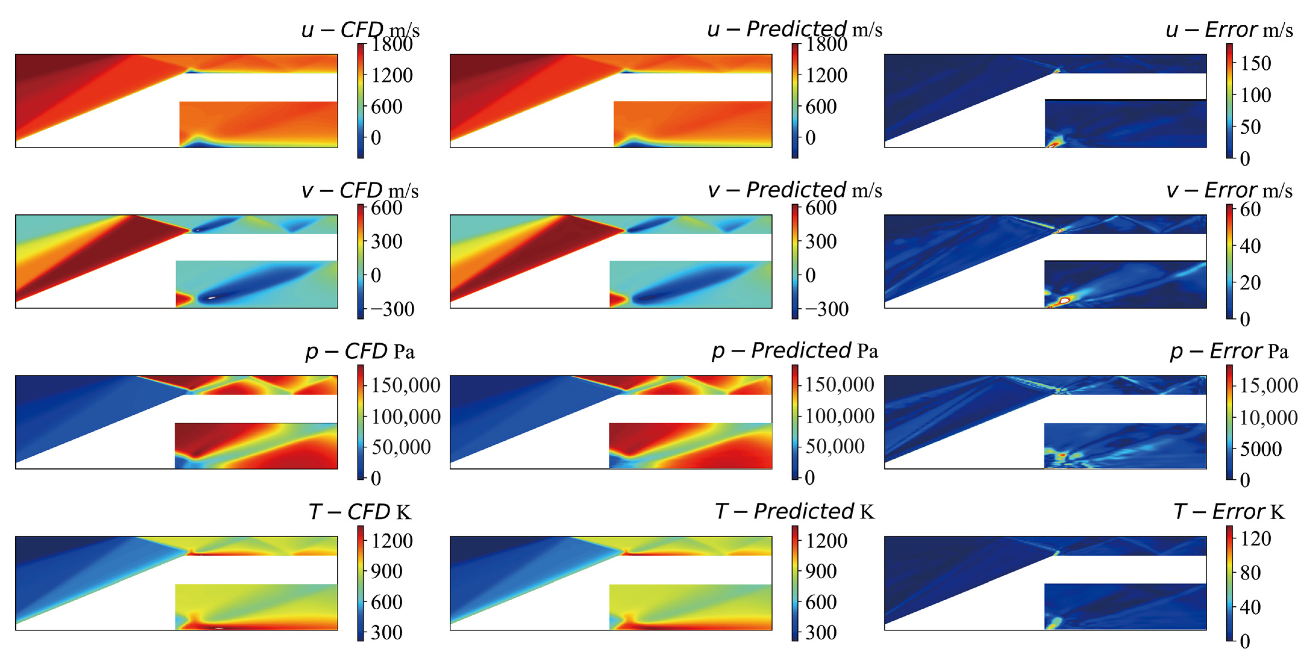
Figure 14 and Figure 15 show typical flow fields for the individuals in the training and testing sets, respectively. Each plot contains twelve subplots, which can be divided into four groups. The subplots in the four rows are the maps of the u velocity, v velocity, static pressure and temperature . The three subplots in each row from left to right are the flow field calculated by CFD, the reconstructed data based on the VAE model, and the absolute error between the CFD and VAE, respectively. We can see that the calculated and reconstructed flow fields are similar in most regions, and the errors are relatively high near shockwaves.

Figure 14.
Typical flow fields reconstructed in the training set.

Figure 15.
Typical flow fields reconstructed in the testing set.
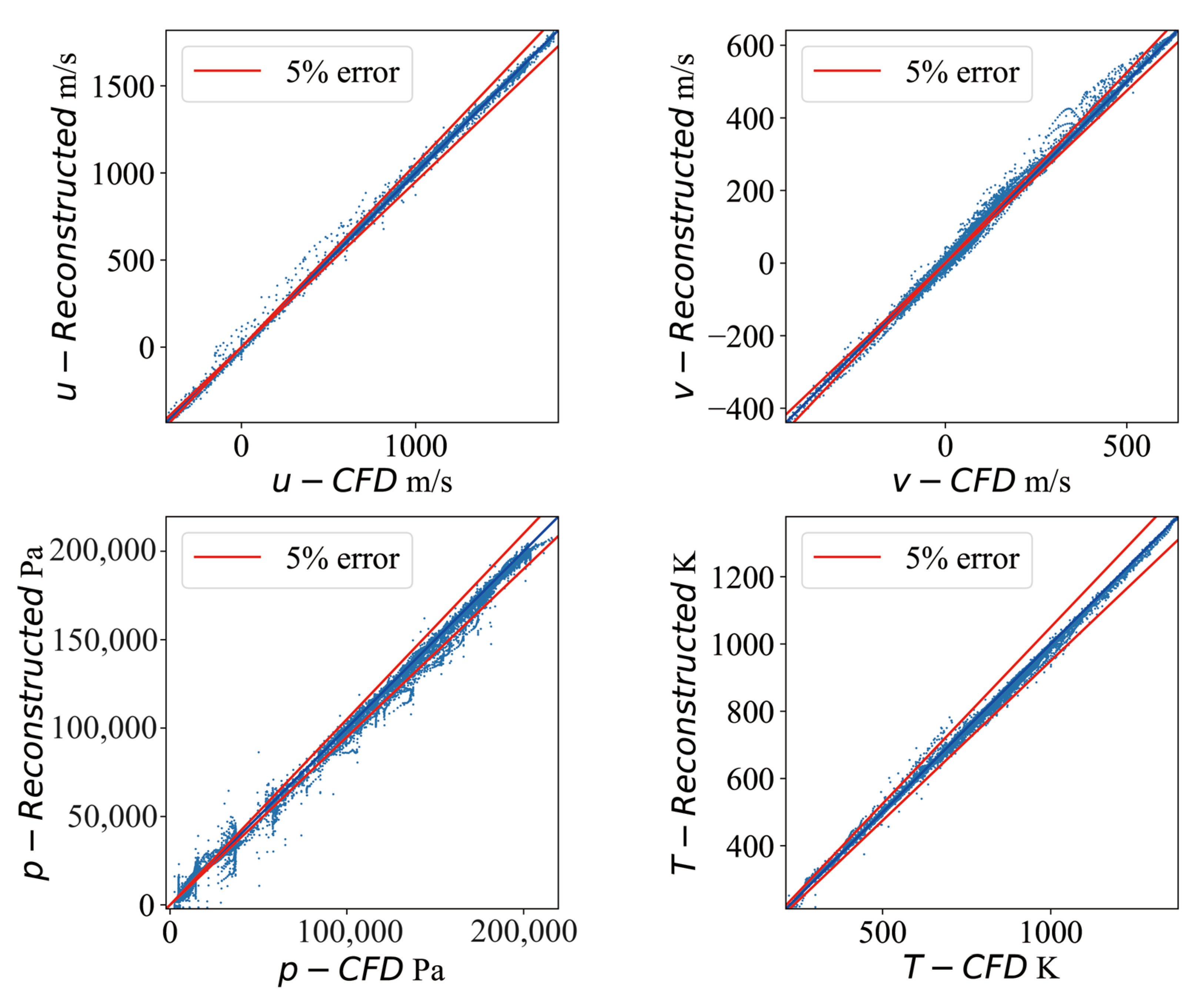
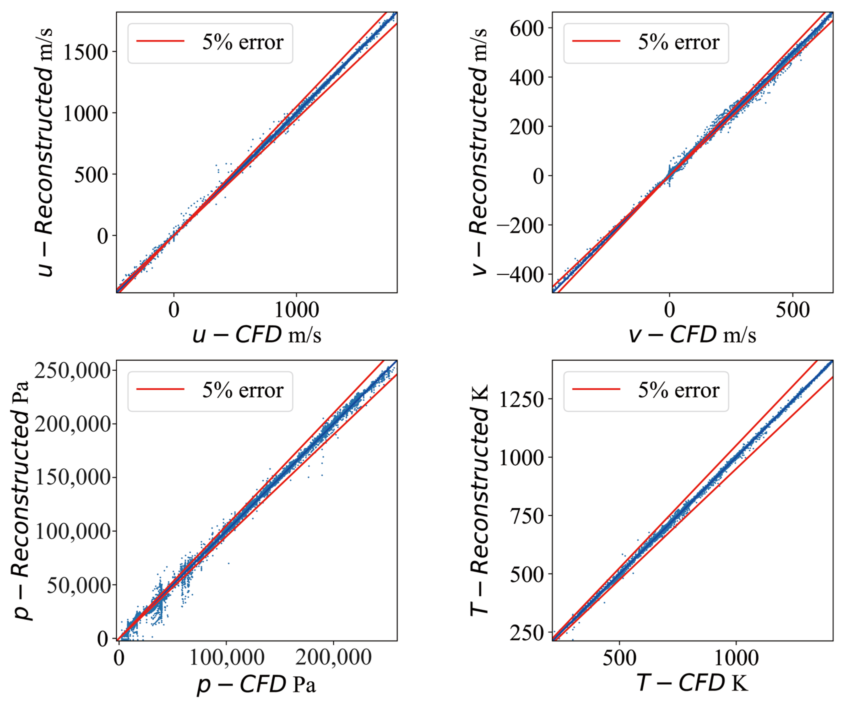
Figure 16 and Figure 17 show the corresponding scatter plots of the flow fields, and each scatter represents the flow data at a grid node. The horizontal coordinates are the values calculated by CFD, and the vertical coordinates are the values reconstructed by VAE. The red lines are the lines of the ±5% errors. We can see that most of the scatters are located inside or near the lines of the ±5% errors. The reconstruction accuracy of the static pressure and vertical velocity has a larger error than the other flow variables. It is consistent with the results in Figure 14 and Figure 15. The vertical velocity and pressure undergo a sudden change besides a shockwave, which makes these two quantities more uneven and discontinuous in spatial distribution.

Figure 16.
Scatter plot of a typical flow field in the training set.
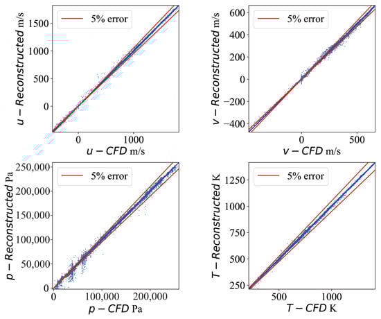
Figure 17.
Scatter plot of a typical flow field in the testing set.
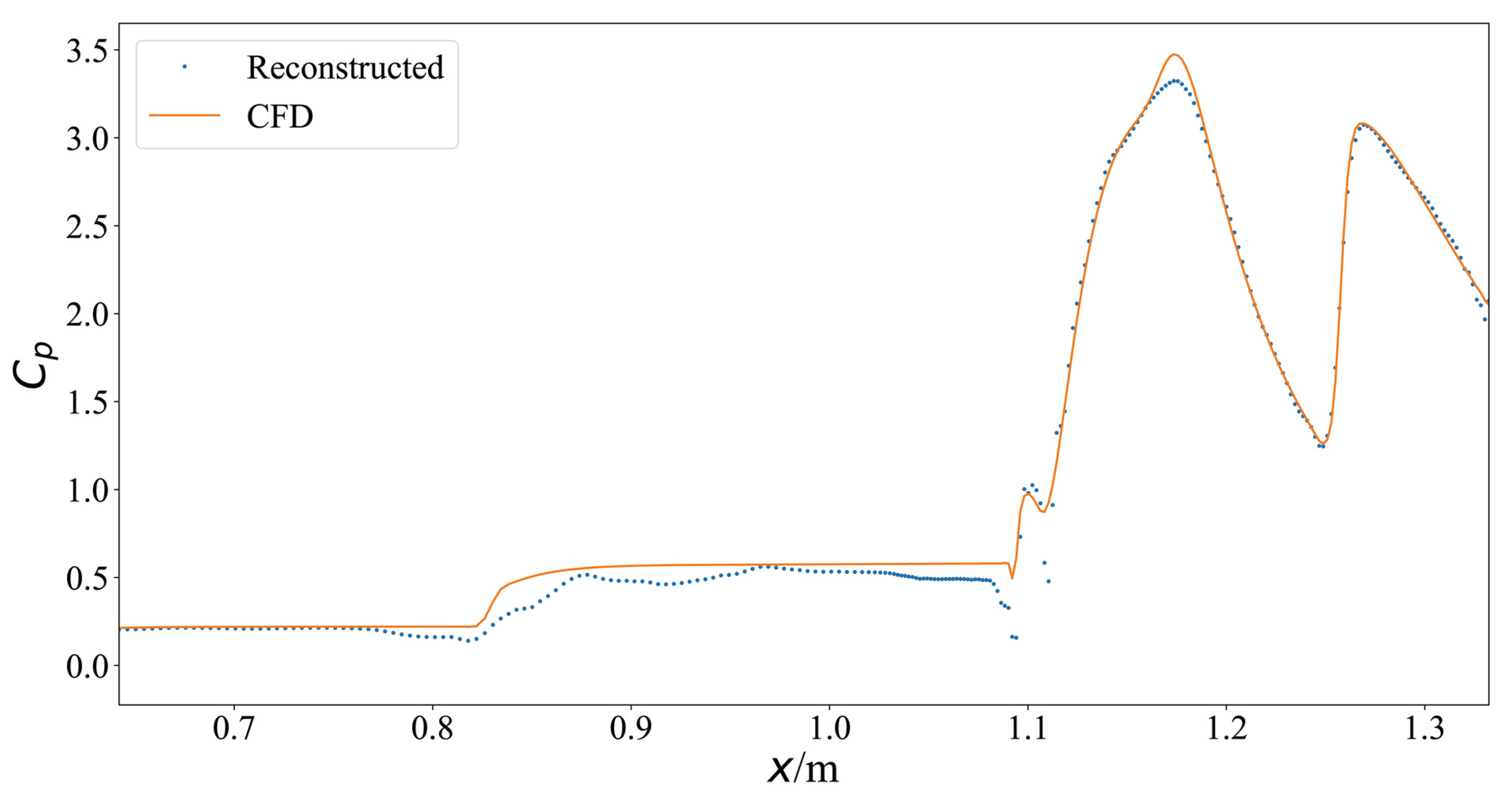
Figure 18 and Figure 19 show the pressure coefficient profile on the compression surface of the typical flow field in the training and testing sets, respectively. The wall pressure is basically well-captured by the VAE reconstruction method. The error is relatively high near the throat, but we are more concerned about the results near the exit of the inlets.
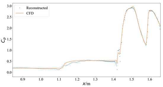
Figure 18.
Pressure coefficient profile on the compression surface of a typical flow field in the training set.
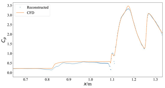
Figure 19.
Pressure coefficient profile on the compression surface of a typical flow field in the testing set.
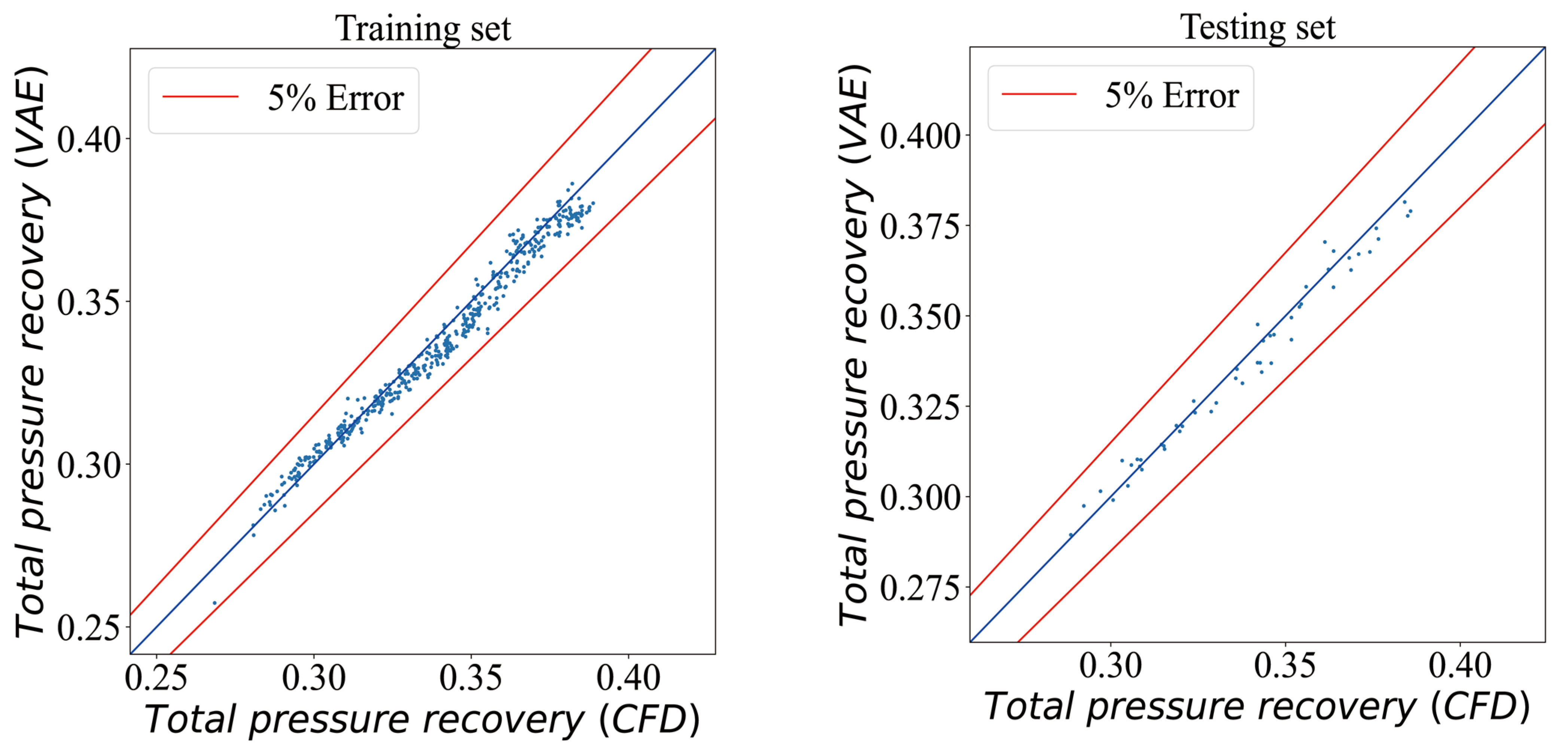
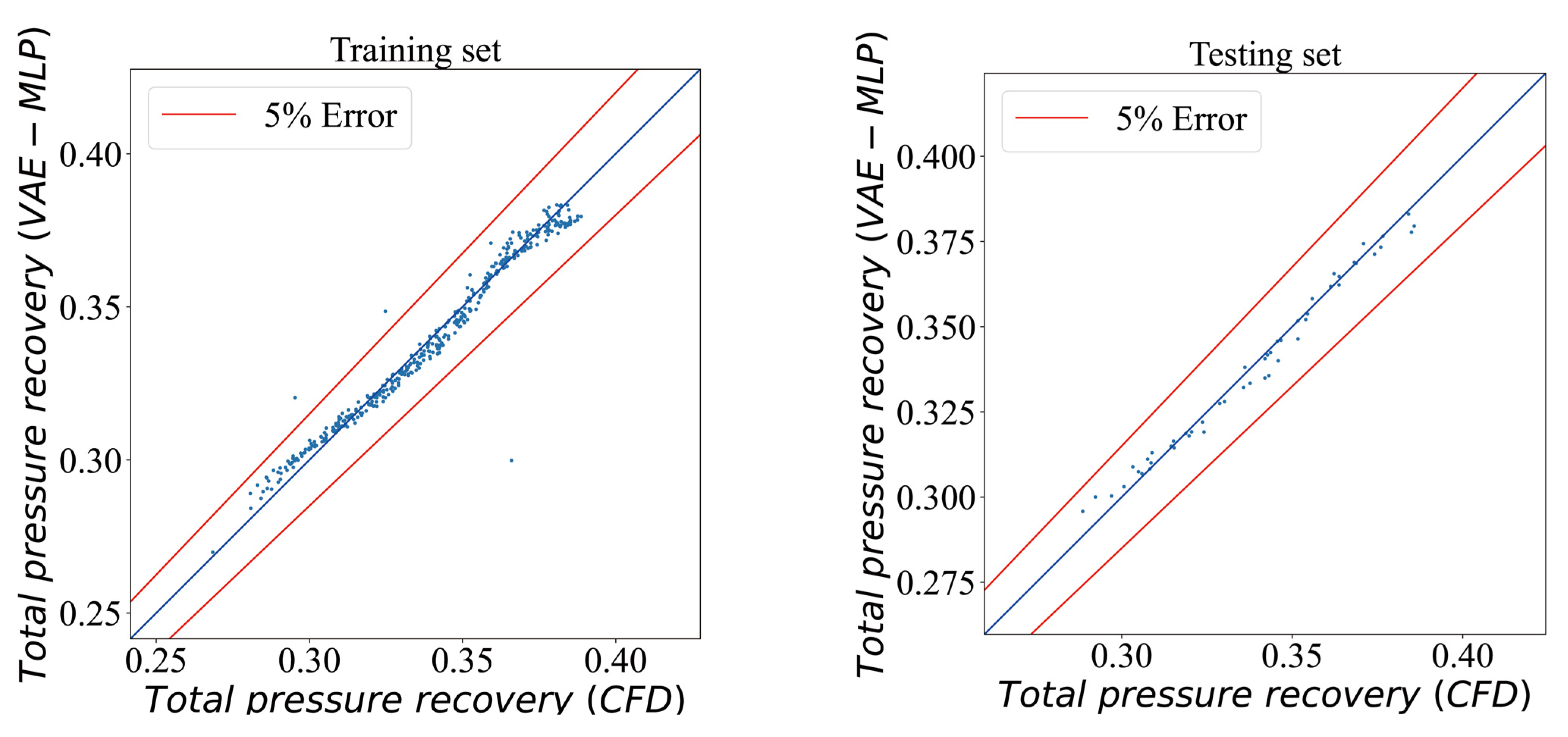
The error distribution of the total pressure recovery of all the reconstructed flow fields is given in Figure 20. The left plot is the training set, which includes 450 training samples; the right plot is the testing set, which includes 50 test samples. Each scatter represents an individual sample, and the horizontal coordinates are the values obtained from the CFD calculations. The vertical coordinates are the reconstructed VAE values. The red lines in the figures are the lines of the ±5% errors.
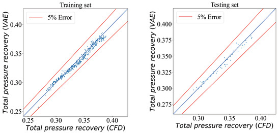
Figure 20.
Error distribution of the total pressure recovery of the reconstructed flow field.
The results in Table 6 show that the correlation coefficients of all the physical quantities between the reconstructed flow field and the CFD flow field are above 0.99, which demonstrates that the accuracy of the flow field reconstruction is relatively high. The flow structure and shockwave pattern of the reconstructed flow field are close to the CFD flow field. The errors of the reconstructed flow field data on most of the grid nodes are within 5% error compared with the CFD values, except for the velocity component . Table 6 and Figure 20 also show that the total pressure recovery of the reconstructed flow fields for all the individual inlets is within 5% error compared to the CFD values. The average error level is less than 2%. The error level of the testing set is also close to that of the training set, indicating that the VAE model has a high generalization capability within the sampling space of the dataset. However, the reconstructed flow field has a significantly larger error near the shockwaves or the flow separation, which indicates that the regions with strong nonlinear effects and complex flow structures are more difficult to capture by the artificial intelligence method than other regions.
5.4. Training of the MLP Model
The MLP model is trained by the Adam optimizer, with an initial learning rate of 0.001 and a decay rate of 1/2 every 1000 epochs. The total training process has 5000 epochs. The batch size is 64. The loss function drop curves are shown in Figure 21.
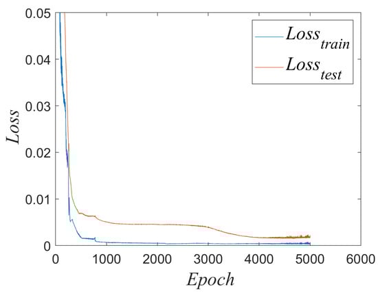
Figure 21.
Loss function drop curves of the MLP model.
5.5. Results of Fluid Field Prediction Based on the VAE-MLP Model
By combining the VAE and MLP models, a hybrid MLP-VAE model is obtained, which can predict the inlet flow field based on the three wedge angles. We continue to use the mean absolute error, correlation coefficient, and relative error of the total pressure recovery between the predicted flow field and CFD to evaluate the accuracy of the prediction model, as listed in Table 7.
Table 7.
Accuracy of the flow field prediction based on the VAE-MLP model.
Figure 22 and Figure 23 show the typical flow field in the training and testing sets, respectively. The subplots in the four rows are the maps of the u velocity, v velocity, static pressure and temperature . The three subplots in each group from left to right are the flow field calculated by CFD, the predicted data based on the hybrid MLP-VAE model, and the absolute error between CFD and the hybrid MLP-VAE model. We can see that the calculated and predicted flow fields are similar in most regions, and the errors are relatively high near shockwaves. The error level of the predicted flow field is roughly equivalent to that of the reconstructed flow field.

Figure 22.
Typical flow fields predicted in the training set.
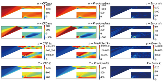
Figure 23.
Typical flow fields predicted in the testing set.
The error distribution of the total pressure recovery of the predicted flow field is given in Figure 24, where the left plot is the training set, and the right plot is the testing set. Each scatter represents an individual sample. The horizontal coordinates are the values obtained from CFD computations. The vertical coordinates are the predicted values given by the VAE-MLP model, and the red lines mark the range of the ±5% errors.
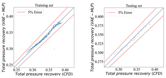
Figure 24.
Error distribution of the total pressure recovery of the predicted flow field.
Comparing the results in Table 6 with those in Table 7, it is found that the overall error level of the predicted flow field obtained by MLP-VAE is comparable to or even slightly reduced compared to that of the VAE reconstructed flow field. This occurs because no reparameterization operation is performed when training the MLP network. Here, the mean of the code distribution, i.e., the value with the maximum probability density of this distribution, is used for training. Figure 24 shows that the MLP-VAE network is also able to predict the inlet total pressure recovery more accurately for most individuals in both the training and testing sets. However, there are three samples with relative errors larger than 5%, which may be due to the cumulative error of the two networks when combined. There was no sample outside the ±5% error range in the testing set.
Since the AI model is based on the probability method, if we run the training model again, the result will not be the same completely. However, the loss function will converge to almost the same value, and the value is usually small, as shown in Figure 13 and Figure 21. Then, the AI model may give a believable and reasonable result for flow field prediction with an acceptable error. In this sense, the AI model is repeatable and is a sufficient surrogate model to replace CFD.
5.6. Computational Cost
The computation times for the different processes in this paper are given in Table 8. The computing platform used for training the VAE is NVIDIA RTX A2000 with CUDA 11.1 and cuDNN8.0.5. The computing platform for training the MLP and CFD calculations is Intel i5-11300H. Although the training of the neural network requires a large amount of data, once the neural network is trained, it can be used repeatedly for the design optimization of the inlet, reducing the marginal cost of the calculations and, thus, significantly reducing the time required for aerodynamic optimization.
Table 8.
Time consumption of different computation processes.
6. Conclusions
This paper implements the flow field reconstruction of a two-dimensional hypersonic inlet based on an artificial intelligence method. First, 500 geometric configurations of the two-dimensional hypersonic inlet are sampled, and the flow field is calculated by CFD to obtain the dataset for training, while the accuracy of the calculation method is verified using the standard model GK-01. Finally, a hypersonic inlet flow field prediction model based on the MLP-VAE network is constructed by training a residual variational autoencoder (VAE) and a multilayer perceptron (MLP).
The results show the following:
- (1)
- The variational autoencoder based on convolutional residual blocks has sufficient depth to characterize the flow fields of hypersonic inlets. The flow field is reconstructed with a good overall accuracy. Even for flow structures with strong nonlinear effects, such as shockwaves, boundary layers, and flow separations, the reconstruction accuracy is well maintained.
- (2)
- The flow field prediction model based on a hybrid MLP-VAE network has good generation capability, performs well on the test set, and can be used for fast predictions of the flow fields of two-dimensional hypersonic inlets.
- (3)
- The neural network surrogate model can significantly reduce the time consumed in calculating the aerodynamic performance and the whole fluid field, thus improving the overall efficiency of aerodynamic optimization and reducing the computational cost.
This is a preliminary attempt to study the flow field reconstruction ability of artificial intelligence. In our future work, the reconstruction method will be further studied and extended to a three-dimensional flow field. The inlet with a lip deflection can also be considered in the dataset.
Author Contributions
Conceptualization, Z.T. and R.L.; software, Z.T.; validation, Z.T.; writing—original draft preparation, Z.T.; writing—review and editing, Y.Z.; supervision, Y.Z.; project administration, Y.Z.; funding acquisition, Y.Z. All authors have read and agreed to the published version of the manuscript.
Funding
This work was supported by the National Natural Science Foundation of China (11872230 and 92152301).
Institutional Review Board Statement
Not applicable.
Informed Consent Statement
Not applicable.
Data Availability Statement
The data presented in this study are available on request from the corresponding author. The data are not publicly available due to privacy.
Conflicts of Interest
The authors declare no conflict of interest.
References
- Sun, G.; Wang, C.; Wang, L.; Tao, J.; Wang, S.; Wang, X.; Zhou, S.; Li, Z.; Hu, Y. Applications and Prospect of Artificial Intelligence in Aerodynamic Design. Civ. Aircr. Des. Res. 2021, 3, 1–9+147. (In Chinese) [Google Scholar]
- Fujio, C.; Ogawa, H. Scramjet Intake Design Based on Exit Flow Profile via Global Optimization and Deep Learning toward Inverse Design. In Proceedings of the AIAA SCITECH 2022 Forum, San Diego, CA, USA, 3–7 January 2022; p. 1408. [Google Scholar]
- Brahmachary, S.; Bhagyarajan, A.; Ogawa, H. Fast estimation of internal flow fields in scramjet intakes via reduced-order modeling and machine learning. Phys. Fluids 2021, 33, 106110. [Google Scholar] [CrossRef]
- Liu, Q.; Luo, Z.; Deng, X.; Wang, L.; Zhou, Y. Numerical investigation on flow field characteristics of dual synthetic cold/hot jets using POD and DMD methods. Chin. J. Aeronaut. 2020, 33, 73–87. [Google Scholar] [CrossRef]
- Sun, F.; Su, W.Y.; Wang, M.Y.; Wang, R.J. RBF-POD reduced-order modeling of flow field in the curved shock compression inlet. Acta Astronaut. 2021, 185, 25–36. [Google Scholar] [CrossRef]
- Vitkovicova, R.; Yokoi, Y.; Hyhlik, T. Identification of structures and mechanisms in a flow field by POD analysis for input data obtained from visualization and PIV. Exp. Fluids 2020, 61, 171. [Google Scholar] [CrossRef]
- Kikuchi, R.; Misaka, T.; Obayashi, S. International journal of computational fluid dynamics real-time prediction of unsteady flow based on POD reduced-order model and particle filter. Int. J. Comput. Fluid Dyn. 2016, 30, 285–306. [Google Scholar] [CrossRef]
- Yousif, M.Z.; Yu, L.; Hoyas, S.; Vinuesa, R.; Lim, H. A deep-learning approach for reconstructing 3D turbulent flows from 2D observation data. Sci. Rep. 2023, 13, 2529. [Google Scholar] [CrossRef]
- Kim, H.; Kim, J.; Won, S.; Lee, C. Unsupervised deep learning for super-resolution reconstruction of turbulence. J. Fluid Mech. 2021, 910, A29. [Google Scholar] [CrossRef]
- Afzali, J.; Casas, C.Q.; Arcucci, R. Latent GAN: Using a latent space-based GAN for rapid forecasting of CFD models. In International Conference on Computational Science; Springer International Publishing: Cham, Switzerland, 2021; pp. 360–372. [Google Scholar]
- Buzzicotti, M.; Bonaccorso, F.; Di Leoni, P.C.; Biferale, L. Reconstruction of turbulent data with deep generative models for semantic inpainting from TURB-Rot database. Phys. Rev. Fluids 2021, 6, 050503. [Google Scholar] [CrossRef]
- Wen, S.; Shen, N.; Zhang, J.; Lan, Y.; Han, J.; Yin, X.; Zhang, Q.; Ge, Y. Single-rotor UAV flow field simulation using generative adversarial networks. Comput. Electron. Agric. 2019, 167, 105004. [Google Scholar] [CrossRef]
- Yousif, M.Z.; Yu, L.; Lim, H.C. High-fidelity reconstruction of turbulent flow from spatially limited data using enhanced super-resolution generative adversarial network. Phys. Fluids 2021, 33, 125119. [Google Scholar] [CrossRef]
- Nista, L.; Schumann, C.D.K.; Grenga, T.; Attili, A.; Pitsch, H. Investigation of the generalization capability of a generative adversarial network for large eddy simulation of turbulent premixed reacting flows. Proc. Combust. Inst. 2022, 39, 5279–5288. [Google Scholar] [CrossRef]
- Hu, L.; Wang, W.; Xiang, Y.; Zhang, J. Flow field reconstructions with gans based on radial basis functions. IEEE Trans. Aerosp. Electron. Syst. 2022, 58, 3460–3476. [Google Scholar] [CrossRef]
- Deng, K.; Chen, H.; Zhang, Y. Flow structure oriented optimization aided by deep neural network. In Proceedings of the Tenth International Conference on Computational Fluid Dynamics (ICCFD10), Barcelona, Spain, 9–13 July 2018. [Google Scholar]
- Wang, J.; He, C.; Li, R.; Chen, H.; Zhai, C.; Zhang, M. Flow field prediction of supercritical airfoils via variational autoencoder based deep learning framework. Phys. Fluids 2021, 33, 086108. [Google Scholar] [CrossRef]
- Dubois, P.; Gomez, T.; Planckaert, L.; Perret, L. Machine learning for fluid flow reconstruction from limited measurements. J. Comput. Phys. 2022, 448, 110733. [Google Scholar] [CrossRef]
- Zalger, J. Application of Variational Autoencoders for Aircraft Turbomachinery Design; Technical Report; Stanford University: Stanford, CA, USA, 2017. [Google Scholar]
- Mrosek, M.; Othmer, C.; Radespiel, R. Variational autoencoders for model order reduction in vehicle aerodynamics. In Proceedings of the AIAA Aviation 2021 Forum, Virtual Event, 2–6 August 2021; p. 3049. [Google Scholar]
- Ando, K.; Onishi, K.; Bale, R.; Kuroda, A.; Tsubokura, M. Nonlinear reduced-order modeling for three-dimensional turbulent flow by large-scale machine learning. Comput. Fluids 2023, 2023, 106047. [Google Scholar] [CrossRef]
- Posch, S.; Gößnitzer, C.; Ofner, A.B.; Pirker, G.; Wimmer, A. Modeling cycle-to-cycle variations of a spark-ignited gas engine using artificial flow fields generated by a variational autoencoder. Energies 2022, 15, 2325. [Google Scholar] [CrossRef]
- Wu, S.; Patel, S.; Ameen, M. Investigation of cycle-to-cycle variations in internal combustion engine using proper orthogonal decomposition. Flow Turbul. Combust. 2023, 110, 125–147. [Google Scholar] [CrossRef]
- Chen, H.; Guo, M.; Tian, Y.; Le, J.; Zhang, H.; Zhong, F. Intelligent reconstruction of the flow field in a supersonic combustor based on deep learning. Phys. Fluids 2022, 34, 035128. [Google Scholar] [CrossRef]
- Laubscher, R.; Rousseau, P. Application of generative deep learning to predict temperature, flow and species distributions using simulation data of a methane combustor. Int. J. Heat Mass Transf. 2020, 163, 120417. [Google Scholar] [CrossRef]
- Häberle, J.; Gülhan, A. Investigation of the Flow Field of a 2D SCRAM Jet Inlet at Mach 7 with optional Boundary Layer Bleed. In Proceedings of the 43rd AIAA/ASME/SAE/ASEE Joint Propulsion Conference & Exhibit, Cincinnati, OH, USA, 8–11 July 2007; p. 5068. [Google Scholar]
- Zhu, C.; Zhang, X.; Kong, F.; You, Y. Design of a three-dimensional hypersonic inward-turning inlet with tri-ducts for combined cycle engines. Int. J. Aerosp. Eng. 2018, 2018, 7459141. [Google Scholar] [CrossRef]
- Kingma, D.P.; Welling, M. Auto-encoding variational bayes. arXiv 2013, arXiv:1312.6114. [Google Scholar]


Disclaimer/Publisher’s Note: The statements, opinions and data contained in all publications are solely those of the individual author(s) and contributor(s) and not of MDPI and/or the editor(s). MDPI and/or the editor(s) disclaim responsibility for any injury to people or property resulting from any ideas, methods, instructions or products referred to in the content. |
© 2023 by the authors. Licensee MDPI, Basel, Switzerland. This article is an open access article distributed under the terms and conditions of the Creative Commons Attribution (CC BY) license (https://creativecommons.org/licenses/by/4.0/).