Abstract
In an effort to address the problem of hypersonic morphing vehicles reaching the target while avoiding no-fly zones, an improved predictor–corrector guidance method is proposed. Firstly, the aircraft motion model and the constraint model are established. Then, the basic algorithm is given. The Q-learning method is used to design the attack angle and sweep angle scheme to ensure that the aircraft can fly over low-altitude zones. The B-spline curve is used to determine the locations of flight path points, and the bank angle scheme is designed using the predictor–corrector method, so that the aircraft can avoid high-altitude zones. Next, the Monte Carlo reinforcement learning (MCRL) method is used to improve the predictor–corrector method and a Deep Neural Network (DNN) is used to fit the reward function. The planning method in this paper realizes the use of a variable sweep angle, while the improved method further improves the performance of the trajectory, including the attainment of greater final speed and a smaller turning angle. The simulation results verify the effectiveness of the proposed algorithm.
1. Introduction
Hypersonic morphing vehicles with a variety of sweep angles have strong maneuverability [1]. The vehicles can perform a variety of missions under different flight conditions with excellent flight performance [2]. The research on this type of vehicle is mainly focused on structural design [3,4,5], trajectory planning [6,7], and attitude control [8,9,10], among which trajectory planning methods represent a very important research topic [3].
A morphing vehicle is a kind of multi-purpose and multi-mode aircraft that can adopt deformations according to the environment and mission requirements. The trajectory, altitude, and speed of the aircraft are adjustable, so the aircraft can be adapted for multiple missions [11,12,13,14]. Most research on morphing aircraft has been carried out at low speeds. In the hypersonic realm, the Defense Advanced Research Projects Agency (DARPA) has proposed the Morphed Aircraft Structure (MAS) project [15]. NASA has proposed the National Aerospace Plane Program and designed a manned, horizontal-takeoff-and-landing, single-stage-to-orbit, airbreathing launch vehicle [16]. Takama, of the Japanese Space Agency, proposed a wave-rider with a wing configuration allowing improved drag lift performance at lower speeds [17]. The study of hypersonic morphing vehicles will be an important research direction in the future.
Trajectory planning for hypersonic vehicles is usually divided into reference trajectory methods [18,19] and predictor–corrector methods [20,21]. Predictor–corrector algorithms have strong online planning ability, and the method and its improvements are often used to guide the re-entry of hypersonic vehicles. Liu et al., in [22], using both the bank angle and attack angle as control variables, obtained much higher terminal altitude precision. M. Xu et al., in [23], proposed a novel quasi-equilibrium glide auto-adaptive guidance algorithm based on the predictor–corrector concept that was able to meet the terminal position constraints. W Li, in [24], proposed a guidance law using an extended Kalman filter to estimate the uncertain parameters for the re-entry flight of the X-33, which was of great value in reconfiguring auto-adaptive predictor–corrector guidance. Z. Liang, in [25], proposed a guidance algorithm based on the reference trajectory and the predictor–corrector algorithm for the re-entry of vehicles that required less computing time, while offering high guidance precision and good robustness. Jay W. McMahon et al., in [26], discussed recent developments in robust predictor–corrector methodologies for addressing the stochastic nature of guidance problems. Current predictor–corrector trajectory planning methods for aircraft usually consist of three steps: (1) determine the attack angle scheme, which is usually a linear transition mode; (2) calculate the size of the bank angle according to the range error; and (3) calculate the bank angle sign according to the aircraft heading. For the hypersonic morphing vehicle in this paper, in order to improve the trajectory performance, it is necessary to design the sweep and angle scheme. The research described above aimed to obtain the trajectory of the hypersonic vehicle and combine the findings with those obtained using other methods in order to improve its trajectory performance. However, for morphing aircraft, this research was not able to provide a guidance scheme; therefore, it is necessary to improve it, which will be the focus of this paper.
The reinforcement learning [27] and deep learning [28] methods have found many applications in trajectory planning algorithms due to their high levels of intelligence and efficiency. Z. Kai, in [29], used a backpropagation neural network trained using the parameter profiles of optimized trajectories taking different dispersions into consideration in order to simulate the nonlinear mapping relationship between current flight states and terminal states. Using this guidance method based on trajectory, the neural network was able to satisfy both the path and terminal constraints well, offering good validity and robustness. Y. Lv, in [30], presented a trajectory planning method based on Q-learning to solve the problem of HCVs facing unknown threats. Brian Gaudet, in [31], used reinforcement meta-learning to optimize an adaptive guidance system suitable for the approach phase of gliding hypersonic vehicles, enabling trajectories to be obtained that would bring the vehicle to the target location with a high degree of accuracy at the designated terminal speed while satisfying heating rate, load, and dynamic pressure constraints. Monte Carlo reinforcement learning [32] is a reinforcement learning approach used to control behavior [33]. This method has been applied to solve many decision problems [34,35]. According to the aforementioned research, reinforcement learning has been proven to be applicable in aircraft guidance and is able to improve the guidance performance and trajectory performance of aircraft. Therefore, in this paper, the use of reinforcement learning is considered with the aim of improving the trajectory planning method in order to obtain a better flight trajectory, thus improving the mission performance of the aircraft.
This article is divided into four sections:
- The motion model of the aircraft is established.
- The basic predictor–corrector algorithm is given. The Q-learning algorithm is used to obtain an attack and sweep angle scheme that enables the crossing of no-fly zones from above. The B-spline curve method is used to solve the locations of flight path points to ensure that the aircraft can cross no-fly zones via these points. The size of the bank angle is solved on the basis of the state error of the aircraft arriving at the target and flight point. The changing logic of the bank angle sign is determined to ensure that the aircraft can fly safely to the target.
- The Monte Carlo reinforcement learning method is used to improve the predictor–corrector algorithm, and a Deep Neural Network is used to fit the reward function.
- The effectiveness of the algorithm is verified by a simulation.
2. Materials and Methods
The aircraft is composed of a body and foldable wings and adopts bank-to-turn (BTT) control with no thrust. The sweep angle of the wing can form three fixed sizes, χ1 = 30°, χ2 = 45°, and χ3 = 80°, respectively, as shown in Figure 1.
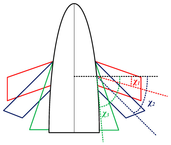
Figure 1.
Top view of the aircraft.
2.1. Aircraft Motion Model
The equations of the motion of the aircraft are established according to [36]. The following assumptions are considered:
- The Earth is a homogeneous sphere;
- The aircraft is a mass point that satisfies the assumption of transient equilibrium;
- The sideslip angle β and the lateral force Z are both zero during flight;
- The Earth’s rotation is not considered.
The equations of motion of the aircraft are given as follows:
where t is the time, r is the distance from the center of the Earth to the aircraft, λ is longitude, ϕ is latitude, v is the aircraft speed, θ is the flight path angle, ψ is the heading angle, L is lift, D is drag, α is the attack angle, σ is the bank angle, and g is the acceleration of gravity. The equations of L, D, and g are as follows:
where cl and cd are the lift and drag coefficients, respectively, and both are determined by α and χ; S is the reference area of the aircraft; q is the dynamic pressure; r0 = 6371 km is the Earth’s radius; and g0 = 9.8066 m/s2 is the acceleration of gravity at the Earth’s surface.
Define s as the flying range:
where (ϕ0, λ0) are the longitude and latitude of the starting point.
2.2. Constraint Model
- Heating rate constraint:
- 2.
- Dynamic pressure q constraint:
- 3.
- Overload n constraint:
- 4.
- No-fly Zone Model
In this paper, two types of no-fly zones are considered. Type 1 is a high-altitude no-fly zone, whose model is a cylinder with a base surface of h = 40 km and a radius of Rn = 300 km. Type 2 is a low-altitude no-fly zone, whose model is a cylinder with a base surface on the ground, a top surface 35 km high, and a radius of 300 km. The two types of no-fly zones are shown in Figure 2. The model of the no-fly zone is given as:
where Δβ = arccos(sinϕnsinϕ + cosϕncosϕcos(λ − λn)) and (λn, ϕn) is the center of the no-fly zone.
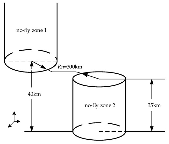
Figure 2.
Sketch of the no-fly zone.
3. Basic Predictor–Corrector Guidance Algorithm
This section introduces the basic predictor–corrector guidance algorithm, which can be used to steer aircraft to reach the desired final position while fulfilling the no-fly zone constraint. The results of the basic algorithm serve as the input of the improved algorithm learning network as a sample, providing training and evaluation data. The basic algorithm includes an attack angle and sweep angle scheme, a flight path point plan, and a bank angle scheme.
3.1. Attack Angle and Sweep Angle Scheme
In this section, the Q-learning algorithm is used to generate the attack angle and sweep angle commands to avoid type 2 no-fly zones.
3.1.1. Q-Learning Principles
In the Q-learning algorithm, the immediate reward rt = R(st,at) is first calculated after state st performs the action. Then, the state-action value function discount value γmaxQ(st+1, a) is calculated for the next state st+1. Then, the value function Q(st,at) in the current state can be estimated. If there are m states and n actions, the Q-table is an m × n matrix.
The objective of the algorithm is to find the optimal strategy π* by estimating the value of the state-action value function Q(st,at) in each state. The rows of the Q-table represent the states in the environment, and the columns of the table represent the actions that the aircraft can perform in each state. In the process of trajectory planning, the environment will provide feedback to the aircraft through reinforcement signals (reward function). During the learning process, the Q-value of the actions that are conducive to completing the task becomes larger with the number of times they are selected, while those not conducive to task completion will become smaller. Through multiple iterations, the action selection strategy π of the aircraft will converge to the optimal action selection strategy π*.
The rule for updating Q-values is:
where maxQ(st+1, a) is the Q-value corresponding to action a with the largest Q-value found in action set A when the aircraft is in state st+1. The iterative Q-value process of the k-th iteration can be obtained as follows:
where α ∈ (0,1) is the learning efficiency to control the rate of learning, i.e., the converging rate is proportional to the magnitude of α. Generally, alpha is set as a constant value. It takes the form of a constant.
Q-learning approximates the optimal state-action value function Q*(s, a) by updating the strategy. Q*(s, a) is the maximum Q-value function among all policies π, represented by:
where Q(st,at) is the state-action value function of all strategies π and Q*(s, a) is the maximum value function, corresponding to the optimal strategy π*. According to the Bellman optimality equation, there is:
where represents the immediate reward obtained by executing action at in state st and reaching state st+1. The greedy strategy is used in this paper.
The basic process of the Q-learning algorithm is as follows:
- Selection of algorithm parameters: α ∈ (0,1), γ ∈ (0,1), and maximum iteration steps tmax;
- Initialization: for all s ∈ S and a ∈ A(s), initialize Q(s, a) = 0 and t = 0;
- For each learning round:
Initialize state st;
Using the strategy π, randomly select at at st, and update Q:
- 4.
- Reach the termination state, or t > tmax.
3.1.2. Q-Learning Algorithm Setting
The Q-learning network takes the aircraft motion model and the environment as inputs to obtain attack and sweep angle schemes. The parameters are set as follows:
- State set
The state in the algorithm needs to be determined based on the flight process. Considering that the range during the flight process usually varies monotonically, using it as a state variable can make the state variables exhibit a one-dimensional trend, which can avoid random changes between state variables and reduce the dimension of state variables to simplify the algorithm. The initial expected range of the aircraft is 6000 km; with every 300 km taken as a state, there can be 20 states: S (S1, S2, …, S20) = {0 km, 300 km, …, 6000 km}. At this time, there is no need to set a state transition function, and the state transition is Si → Si+1 (i = 1 … 19).
- 2.
- Action set
Set the action set to Ai = (χ, α), which includes the sweep angle and attack angle. The sweep angles include 30°, 45°, and 80°, and the range of attack angle values is 5°~25°. Taking 5° as the interval, five conditions can be taken, namely 5°, 10°, 15°, 20°, and 25°, respectively, to obtain 15 actions. The action set can be expressed as A = {A1(30°, 5°), A2(30°, 10°), …, A15(80°, 25°)}.
- 3.
- Reward function
The setting of the reward function is crucial, as it relates to whether the aircraft can avoid no-fly zones and reach the target. The rationality of the reward directly affects learning efficiency. Based on the environment, the reward function is set as follows:
where Rb and Rn are the rewards obtained by the aircraft when entering the no-fly zone and during normal flight, respectively, Rb is set as a constant less than 0 to guide the aircraft to avoid the no-fly zone, and Rf is set as a reward related to the aircraft’s velocity to enable the aircraft to store more velocity when reaching the target; Rt is the reward for the arrival to the target, and setting it as a constant greater than 0 can guide the aircraft to reach the desired range; and Rc is the reward when the aircraft does not meet flight constraints, and setting it to a constant less than 0 can ensure the safety of the aircraft’s flight performance.
In this section, the avoidance of type 2 no-fly zones has been achieved through the attack and sweep angle scheme, while the type 1 zones need to be avoided through lateral flight. The following is the lateral trajectory scheme. The attack and sweep angle schemes obtained in this section will be provided as inputs to the lateral planning algorithm.
3.2. Flight Path Point Plan
For the no-fly zones present in the environment, it is necessary to design avoidance methods. In the analysis in the last section, it can be seen that the type 2 zone can be avoided by pulling up the trajectory, while the type 1 zone cannot. Therefore, the type 1 zone needs to be avoided through lateral maneuvering, and it is necessary to plan the lateral trajectory. The B-spline curve is used to obtain flight path points, and the lateral guidance of the aircraft is realized by tracking the points.
3.2.1. B-Spline Curve Principle
The B-spline curve is composed of a starting point, an ending point, and control points. By adjusting the control points, the shape of the B-spline curve can be changed. B-spline curves are widely used in various trajectory planning problems due to their controllable characteristics [37]. The B-spline curve is expressed as:
where Pi is the control point of the curve, P0 is the starting point, Pn is the endpoint, and n is the order of the curve. As long as the first and last control points of the two B-spline curves are connected and the four control points at the connection are collinear, it can be ensured that the curve has the same position at the connection and the first derivative of the curve is the same. The concatenated curve will still be a B-spline curve. The lateral trajectory planning of the aircraft can be realized using this property.
3.2.2. No-Fly Zone Avoidance Methods
Considering the horizontal environment model, the no-fly zone is projected from a cylinder in a circle. A 2D B-spline curve is designed that satisfies the constraint, and then flight path points are obtained according to curve control points. The planning method is divided into the following steps:
- 1.
- Based on the location of the circles, choose an appropriate direction to obtain the tangent points of the circles, and then select different combinations of tangent points to obtain the initial control points. If the initial point and target line pass through the threat zone, at least one tangent point is selected as the control point, and at most one tangent point is selected for each zone.
- 2.
- Augment the initial control point set. The initial augmentation control point is located on the initial heading to ensure the initial heading angle and the intermediate augmented control points are located on both sides of the tangent points; then, the control point set is obtained. The initial position P0 and end position Pn of the curve correspond to the initial position of the aircraft and the target. In order to ensure that the aircraft can avoid the threat area, the aircraft must be on the other side of the threat area’s tangent line. Therefore, the B-spline curve is designed to be tangent to the circle of the zone. According to the characteristic of the curve, the tangent point can be the middle point of three collinear control points. Then, adjust the distance d1 and d2 between the two adjacent control points to control the curvature of the curve near the tangent point so that it does not intersect the circle, as shown in Figure 3. In the figure, P0~P4 are the control points, and the red spline curve is tangent to the no-fly zone, preventing the curve from crossing the zone.
 Figure 3. Control point near the no-fly zone.
Choose the tangent point (P2) of the circle as the initial control point and augment the two control points (P1, P3) on both sides of the tangent point. The augmented control points are given by the distance (d1, d2) from the tangent point.
- 3.
- Take the distance between the tangent point and the augmented point as the optimization variable. Take the spline curve length and mean curvature as the performance indicators. The optimal curve is obtained through a genetic algorithm, and the control points are obtained. The optimization model is as follows:
It should be noted that the curve is not the lateral trajectory of the aircraft, so its length cannot represent the flight range and its curvature cannot represent the overload of the aircraft. However, as characteristics of the curve, these elements can be used to evaluate the performance of the curve. The optimal B-spline curves are obtained through optimization. Curves that cross the no-fly zones are discarded, and then the one with the best performance index from all curves is selected.
- 4.
- Simplify the control points to obtain the flight path points.
The simplification rules are as follows. (1) Simplify from the beginning point to the endpoint and delete the augmented control point of the starting point. (2) If multiple points are located on one line segment, delete the intermediate points and leave the two endpoints. (3) If there are four consecutive control points (P0~P3), after deleting the second control point P1, the angle of connecting lines through P0-P2-P3 is bigger than the original and does not cross the no-fly zone, so delete the second control point P1. (4) When the simplification is repeated until two consecutive point sets are identical, the simplification process is finished.
3.3. Bank Angle Scheme
The bank angle scheme includes the size scheme and the sign scheme, obtaining the value and the sign of the bank angle, respectively.
3.3.1. Bank Angle Size Scheme
The bank angle size scheme is achieved through the predictor–corrector algorithm. First, the horizontal error of the flight path point is predicted based on the attack and sweep angle scheme, and then the amplitude and size of the bank angle are corrected.
Based on the attack angle, sweep angle, and the initial bank angle, the equation of motion is integrated until the vehicle reaches the next path point. Then, the latitude position error eϕ and the velocity error ev are obtained. Using the secant method, the amplitude of the bank angle |σmax| is corrected by ev, and the size of the bank angle |σ| is corrected by eϕ. When the aircraft is between two points Pn and Pn+1, there is a relationship as shown in Figure 4.
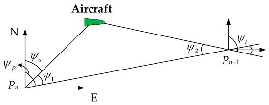
Figure 4.
Flight heading angle.
The correction process for the size of the bank angle is given as follows:
- (1)
- Taking an initial value σ0 = 20°, integrate the equations of motion to the longitude of the target, and calculate the ev.
- (2)
- For intermediate path points, if ev is less than 10% of the expected speed, correction is completed; otherwise, σ0 = σ0 + sgn(ev), so return to step (1). For the trajectory endpoint, no correction is required, so take σ0 = σ0 + 1.
To avoid large overshoots of position when the aircraft passes through the path point line, the bank angle size is set to be related to ψ1 and ψ2 in Figure 4. This will reduce the bank angle as the aircraft approaches the path point connection line. The scheme is as follows:
where ke > 0 is the coefficient of the bank angle error, which is determined by eφ. The correction process is as follows:
- (1)
- Taking an initial σ0 satisfying |σ0| < |σmax|, obtain ke1 at this time, integrate the motion equations to the longitude of the target and obtain eϕ1.
- (2)
- Taking σ0 = 0 and ke0 = 0 at this time, integrate the equations of motion to the longitude of the next path point and calculate eϕ0.
- (3)
- ke is obtained using the correction equation:
- (4)
- Integrate the motion equations to the longitude of the target and then calculate eϕ.
- (5)
- If eϕ < 0.01, the correction process is completed; otherwise, eϕ1 = min(eϕ1, eϕ0). Update ke1 and take ke0 = ke, eϕ0 = eϕ; return to step (3).
The above is the scheme of the bank angle size.
3.3.2. Bank Angle Sign Scheme
After obtaining the set of flight path points, each point should be tracked to ensure the correct heading of the aircraft. At this time, it is necessary to give the change rule of the bank angle sign.
The heading angle ψp of the connecting line at points (λ1, ϕ1) and (λ2, ϕ2) is:
where ψ1 = ψs − ψp and ψ2 = ψt − ψp are the heading angle of the aircraft and the connecting line between the front and back path points. It is known that ψ1 and ψ2 have different signs. If the aircraft is located on the left side of the path point line (as shown in Figure 4), then ψ1 < 0 and ψ2 > 0. The aircraft needs to increase the heading angle, and the bank angle is a positive sign. If the aircraft is located on the right side of the waypoint line (as shown on the other side), then ψ1 > 0 and ψ2 < 0. The aircraft needs to reduce its heading angle, and the bank angle is a negative sign. The bank angle’s sign-changing logic is:
where sgn(·) is a sign function.
The above is the entire process of the basic predictor–corrector guidance algorithm.
4. Improving Predictor–Corrector Methods
In this paper, the MCRL method [38] is used to improve the basic predictor–corrector algorithm. The Monte Carlo reinforcement learning algorithm is used to improve the predictor–corrector algorithm, and the basic algorithm is used to obtain the sample for training the MCRL network. According to the reward calculated by the errors of the aircraft state reaching path points, the optimal control command is trained. The reward function solution is fitted by the DNN to improve the efficiency of the algorithm.
4.1. Monte Carlo Reinforcement Learning Method
In the MCRL method, the learning sample is obtained by a large number of model calculations, and the average reward is taken as the approximate value of the expected reward. The method directly estimates the behavior value function in order to obtain the optimal behavior directly via the ε-greedy strategy.
4.1.1. MCRL Principle
The behavior value function Q is:
where R is the reward of one step.
For the model-free MCRL method, information needs to be extracted from the samples, and the average reward of each state st is calculated as the expected reward. It is necessary to use strategy π to generate multiple complete trajectories from the initial state to the termination state and calculate the reward value of each trajectory. The solution equation is as follows:
where a1, a2, … are discount coefficients and a1 + a2 + … = 1.
The algorithm adopts the ε-greedy strategy for action selection. The strategy randomly selects an action from the action set with a probability of ε and changes it to 1 − ε. Assuming that there are n actions, the probability that the optimal action is selected is 1 − ε + ε/n, and the equation of the ε-greedy algorithm is:
Using this strategy, the probability of selecting each action in the action set is non-zero, which increases the probability of selecting the optimal action while ensuring sufficient exploration.
In this paper, the importance sampling method is used to evaluate strategy π using strategy π’. When the ε-greedy strategy is adopted to evaluate the greedy strategy, the equation for updating the action value function is:
The MCRL process is shown in Algorithm 1.
| Algorithm 1: MCRL algorithm |
| Input: environment E, state space S, action space A, initialization behavior value function Q. Output: Optimal strategy π *. Initialize Q(s, a) = 0, total reward G = 0 For k = 0, 1, …, n Execute in E ε-greedy strategy π’generates trajectory For t = 0, 1, 2, …, n End for |
| End for |
4.1.2. MCRL Method Settings
The MCRL method includes state sets, action sets, and reward functions. The parameters are set as follows:
- (1)
- State set
There are two waypoints on the flight trajectory, which can be divided into three sections: starting point → path point 1 → path point 2 → endpoint. In the MCRL method, the algorithm state is the flight state set Sfly = (h, λ, ϕ, v, θ, ψ). At this point, the state set consists of three states, which are S(S1, S2, S3) = {starting point, path point 1, path point 2}. There is no need to set a state transition function, and the state transition is Si → Si+1(i = 1, 2, 3).
- (2)
- Action set
The action Ai= (|σmax|i, kei) is designed, including the amplitude and error coefficient of the bank angle. The value of the bank angle amplitude ranges from 0° to 30°, with 31 groups at an interval of 1°. The error coefficient of the bank angle has different ranges in different trajectory sections. The coefficients ke1 and ke2 range from 0 to 20, with 21 groups at an interval of 1, and ke3 ranges from −0.3 to 0.1, with 41 groups at an interval of 0.01. The action set A = {A1, A2, A3} is obtained.
- (3)
- Reward function
The reward function considers three states when the aircraft reaches the target: the latitude error eϕ, the speed vt, and the heading angle error eψ = ψ − ψLos. The equation of the reward function is:
where μ is the offset coefficient; σ1, σ2, and σ3 are the scaling coefficients b1, b2, and b3 are the weight coefficients; and b1 + b2 + b3 = 1. When the error eϕ does not meet the error boundary, it is considered that the aircraft cannot reach the expected position, and the reward is 0.
4.2. Deep Neural Network Fitting the Reward Function
- DNN principle
This article uses a DNN to fit the reward function. The basic structure of the DNN, which can be divided into the input layer, hidden layer, and output layer, is shown in Figure 5. In the figure, ω is the weight coefficient; b is the threshold, with a superscript representing the number of layers; and a subscript representing the number of neurons. Assuming that the activation function is f (), the number of neurons in the first hidden layer is m and the output is a, and then the output of layer l is:
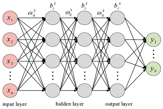
Figure 5.
Structure of the DNN.
- 2.
- DNN settings
The network consists of three hidden layers with ten neurons in each hidden layer. The network structure is “ninput-10-10-10-noutput”, where “ninput” and “noutput” are the quantities of input and output determined by the sample. Then, the sample data are mapped in [–1, 1] using the normalization equation:
In this paper, the feedforward backpropagation network, backpropagation training function, gradient descent learning function, average data performance variance, and tansig transfer function are selected. The tansig function equation is:
It takes four passes from the input layer to the output layer. After learning, four weight matrices (W1, W2, W3, W4) and four threshold matrices (b1, b2, b3, b4) will be obtained. For input x, the network outputs y:
5. Simulation
The initial altitude of the aircraft is h0 = 68 km; the longitude and latitude are (λ0 = 0°, ϕ0 = 0°); the velocity is v0 = 5300 m/s; the initial ballistic inclination angle of the aircraft, the attack angle α0, and the bank angle σ0 are all 0°; the initial heading angle is ψ0 = 85°; the target point is located at (λt = 53.8°. ϕt = 5.4°); and the expected range s = 6000 km. There are two type 1 no-fly zones, with centers located at (23°, 4.5°) and (37°, 1.5°), and two type 2 no-fly zones, with centers located at (30°, 3°) and (45°, 6°). C language was used in the simulation, and the simulation environment was vs2021.
5.1. Simulation of Attack and Sweep Angle Scheme
According to the environment, two type 2 zones are set up, and σ = 20°, α = 0.01, and γ = 0.99 are taken based on engineering experience. The change in total reward after 50,000 studies is shown in Figure 6 and the flight process statuses are shown in Figure 7, Figure 8, Figure 9 and Figure 10.
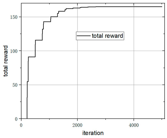
Figure 6.
Total reward curve.
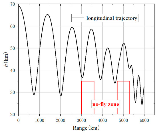
Figure 7.
Longitudinal trajectory.
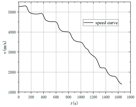
Figure 8.
Speed curve.
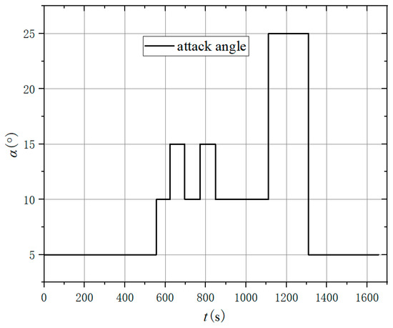
Figure 9.
Attack angle curve.
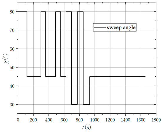
Figure 10.
Sweep angle curve.
The total reward increases rapidly before 20,000 iterations; then, the increase tends to converge, and the value is about 165. Because the reward for each (st, at) is set to be less than 1 and some actions cannot be selected, the more actions that can be selected, the greater the value, but it will not be greater than 300(st × at).
The trajectory shown in Figure 7 could avoid type 2 no-fly zones, and the total reward of the algorithm tends to converge after 30,000 learning iterations. The longitudinal trajectory of the aircraft can avoid the no-fly zones and fly to a range of 6000 km. At a range of 3000 km and 4500 km, the aircraft changes both the attack and the sweep angle. And because the height of the aircraft at this time is less than 40 km, there is a relatively large air density, which can generate large lift, so the height of the aircraft began to increase. The trajectory rose to more than 35 km, successfully crossing the no-fly zone. Figure 8 is the speed curve. In this curve, the time of flight is 1670s and the final speed is 1350. The speed decreases because the energy decreases throughout the flight, but the speed of this decrease alternates between fast and slow. This is because when the height of the aircraft increases, the kinetic energy is converted into gravitational potential energy, and the speed decreases rapidly. When the height of the aircraft decreases, the gravitational potential energy of the aircraft is converted to kinetic energy. Although the aircraft is subjected to drag, the speed change is still small. The schemes of the attack and sweep angle are shown in Figure 9 and Figure 10. The changes in the two angles determine the aerodynamic lift and drag during flight, which make the altitude of the trajectory change. It is under the action of these two angles that the aircraft can fly over the no-fly zones.
5.2. Flight Path Point Planning Results
Based on the method in Section 3.2, the evaluation functions J of these eight trajectories are shown in Table 1. All curves generated using single and double tangent points are shown in Figure 11.

Table 1.
B-spline trajectory evaluation table.
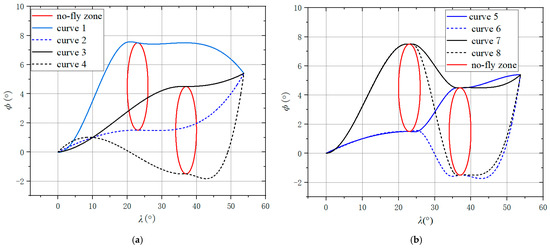
Figure 11.
B-spline curve trajectory. (a) Single tangent point curve; (b) Double tangent point curve.
It can be seen that both the single and double tangent points generate four curves, and trajectory 5 is obtained as the optimal solution. The augmented and simplified points are shown in Table 2.

Table 2.
Flight path point table.
Now, the path points required for trajectory planning are obtained.
5.3. Simulation of Network Training
- DNN network training
Set the maximum number of iterations of network training to 1000, the minimum performance gradient to 10−7, the maximum number of confirmed failures to 6, the target value of error limit to 0, and the learning rate to 0.05. The parameter settings in the reward value function are shown in Table 3 and are based on engineering experience and the order of magnitude estimate.

Table 3.
Reward function parameter settings.
The learning effect of the training process is shown in Figure 12 and Figure 13. Part of the sample (data from group 600 to group 800) was randomly selected for testing, and the test results were compared with the sample results, as shown in Figure 14.
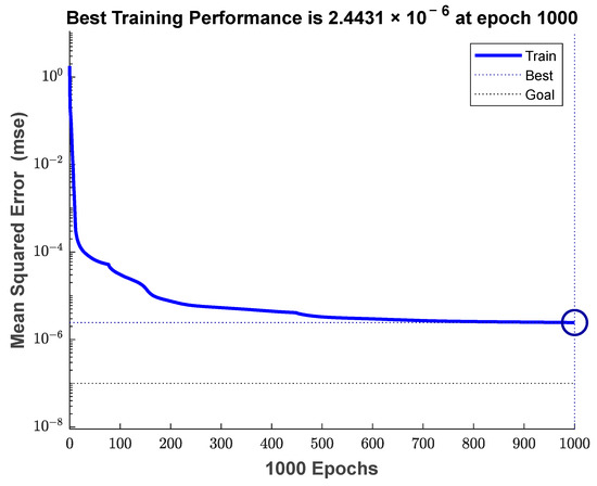
Figure 12.
Mean squared error.
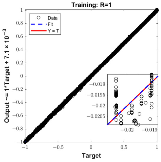
Figure 13.
Sample regression curve.
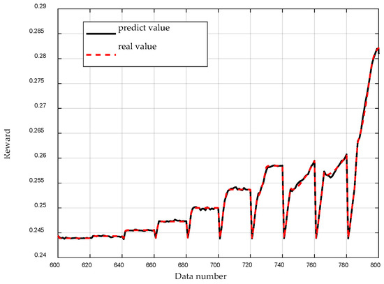
Figure 14.
Comparison of test and sample rewards.
In the above results, it can be seen that when the number of iterations reaches 1000, the mean square error of the network converges to 9.2425 × 10⁻⁷, which meets the requirement. The sample regression performance indicator R = 1 indicates strong data regression. As shown in Figure 14, the test results basically coincide with the sample. The above results demonstrate the good fitting ability of the DNN, which can achieve an accurate and fast estimation of the rewards.
In Figure 12, it can be seen that when the number of iterations reaches 1000, the mean square error of the network converges to 9.2425 × 10⁻⁷, which meets the requirement. The sample regression performance indicator R = 1 indicates strong data regression, as shown in Figure 13. As shown in Figure 14, the test results basically coincide with the sample. The above results demonstrate the good fitting ability of the DNN, as it can achieve an accurate and fast estimation of the rewards.
- 2.
- MC Algorithm Simulation
In this paper, α = 0.01, ε = 0.1, and γ = 0.99 are set based on engineering experience. After 50,000 studies, the total reward is shown in Figure 15.
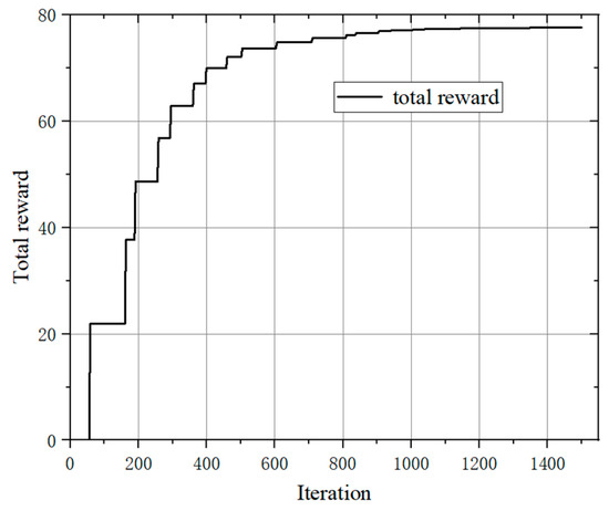
Figure 15.
Total reward of the MC algorithm.
The total reward increases rapidly before 800 iterations; then, the increase tends to converge after 1000 iterations. The value is about 78.
5.4. Simulation of the Trajectory Planning Algorithm
5.4.1. Scenario 1
In this scenario, the basic and improved algorithms are used for simulation. The parameters of the bank angle are shown in Table 4, which are given by the order of magnitude estimate.

Table 4.
Bank angle command.
The results are shown in the following figures. Among them, trajectory 1 is the basic algorithm’s result, and trajectory 2 is the improved algorithm’s result.
According to the 3D, longitudinal, and lateral trajectories shown in Figure 16, Figure 17 and Figure 18, the aircraft can reach the target using both methods. The trajectories can cross two type 2 zones (light red) from the top, avoid two type 1 zones (dark red) from the side, and fly through the planned path points. These results indicate the effectiveness of the attack and sweep angle scheme, path point curve scheme, and bank angle scheme. The improved method has a shorter trajectory. In both cases, the improved method takes less time and the trajectory makes fewer turns. Figure 19 shows the bank angle curves, which show that there is a difference between the two methods: the trends are the same but the values are different. It can be considered that the improved method is an optimal solution of the basic method. The basic method sets a gradient optimization artificially and outputs the result if the aircraft reaches the target. In the process of MCRL, the whole process is deemed optimal, so its trajectory is better. Figure 20 is the speed curve, and it can be seen that the final velocity of the improved method is 1350 m/s, which is bigger than the 700 m/s velocity of the basic method. The trend of velocity change is the same as in Figure 8. Due to the same attack and sweep angle command, the flight path angles shown in Figure 21 of the two trajectories are almost the same. It can be seen in the figure that the flight path angle curve has oscillatory changes, but the absolute value is not greater than 10°, indicating that the altitude of the aircraft will not change very dramatically. The difference in bank angle makes the heading angle vary greatly, as shown in Figure 22. The change in the heading angle of the basic method is larger. The heading angle of trajectory 1 changes more dramatically after 900 s and reaches 156° at the end time, while trajectory 1 is only 110°, which indicates the advantage of the improved method. According to the h-v flight profile in Figure 23, it can be seen that the h-v curves of the aircraft are all above the three overloads, heating rates, and dynamic pressure curves, indicating that the trajectories obtained by both methods meet the performance constraints of the aircraft. Finally, the improved method obtains a better end state for the trajectory.
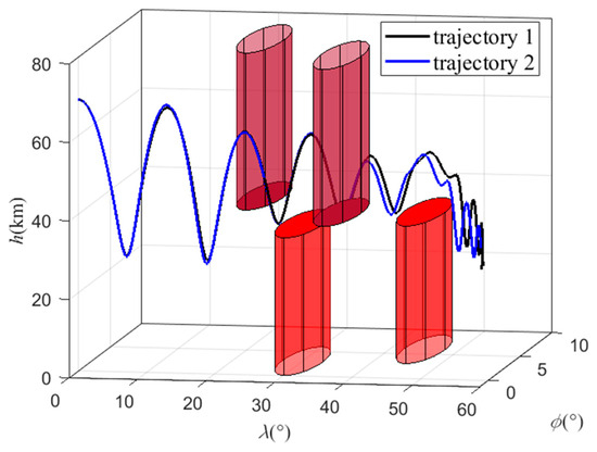
Figure 16.
Three-dimensional trajectory.
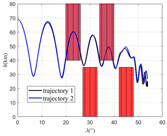
Figure 17.
Longitudinal trajectory.
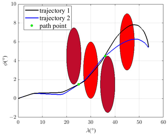
Figure 18.
Lateral trajectory.
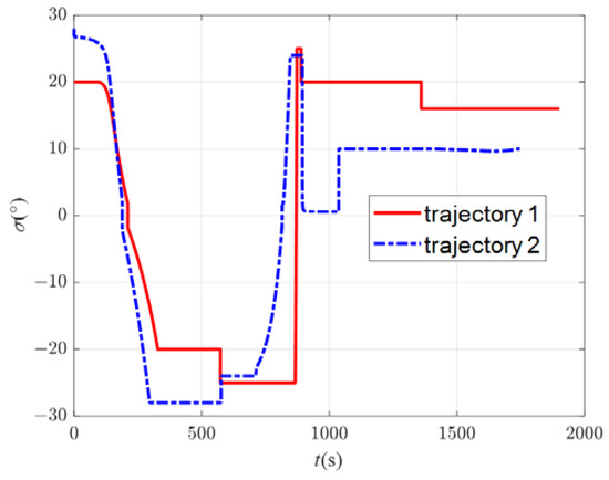
Figure 19.
Bank angle curve.
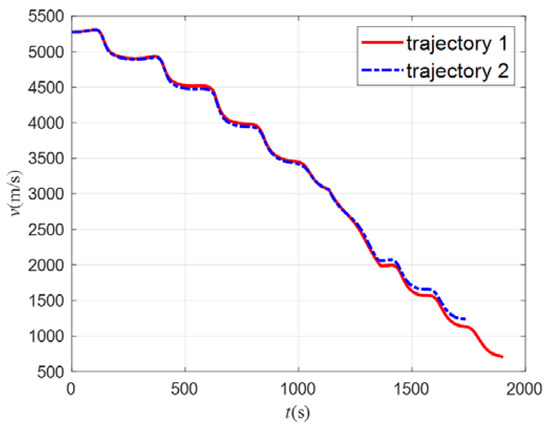
Figure 20.
Speed curve.
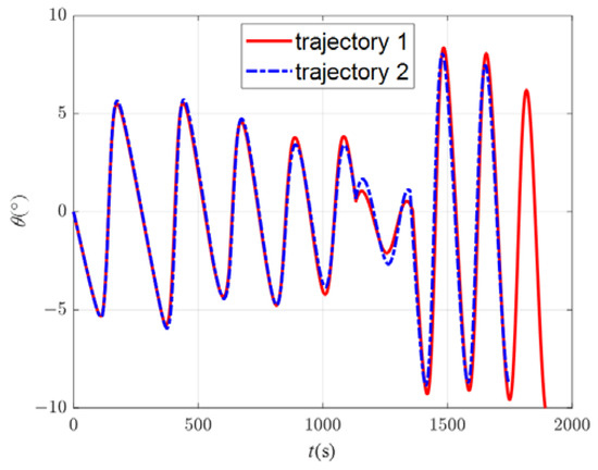
Figure 21.
Path angle curve.
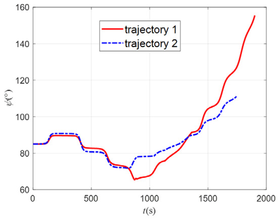
Figure 22.
Heading angle curve.
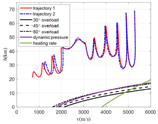
Figure 23.
H-V profile.
5.4.2. Scenario 2
In order to explore the influence of changing the swept wing to avoid the no-fly zones on the trajectory, there are two trajectories in this scenario. In trajectory 1, the improved algorithm is used for simulation. In trajectory 2, the aircraft avoids the no-fly zones only through lateral maneuvers; that is, only the bank angle is adjusted, while the attack angle is fixed at 5° and the sweep angle is fixed at 45° during flight, producing the maximum lift–drag ratio. The locations of the no-fly zones are different in scenario 2. There are two type 1 no-fly zones, with centers located at (15°, 4.5°) and (50°, 1°), and two type 2 no-fly zones, with centers located at (25°, 4.5°) and (35°, 4.5°). All the parameters of this scenario are shown in Table 5. The flight path point is obtained via the B-spline curve scheme, and the command of the bank angle is obtained via the MCRL method.

Table 5.
Command of the trajectories.
According to the 3D, longitudinal, and lateral trajectories shown in Figure 24, Figure 25 and Figure 26, the aircraft can reach the target and avoid the no-fly zones using both methods. Trajectory 1 can cross two type 2 zones (light red) from the top and avoid two type 1 zones (dark red) from the side. Trajectory 2 can avoid all zones from the side. Both trajectories can fly through the planned path points. Because trajectory 2 flies around all the no-fly zones, its trajectory has a larger turn than trajectory 1. Figure 27 shows the curves of the attack angle, and Figure 28 shows the curves of the sweep angle. The curve of trajectory 1 changes in order to avoid the type 2 zones, which are obtained via Q-learning. The curves of trajectory 2 are fixed sets. Figure 29 shows the bank angle curves, which are obtained using the bank angle scheme. Figure 30 shows the speed curves, and it can be seen that the final velocity of trajectory 1 is 1650 m/s, which is smaller than the 2980 m/s velocity of trajectory 2. The trend of velocity change is the same as in Figure 8. This indicates that in order to fly over the top of the no-fly zones, more energy must be consumed, so the speed will be lowered, and the trajectory will take more time. The flight path angles of the two trajectories are shown in Figure 31. It can be seen in the figure that the flight path angle curves both show oscillatory changes. The absolute value of trajectory 1 is not greater than 8°, while the absolute value of trajectory 1 is not greater than 5°. This is because trajectory 1 needs to fly higher to avoid the no-fly zone, so its path angle will be larger to raise the altitude of the trajectory, which causes the decrease in speed. The heading angle is shown in Figure 32. The change in the heading angle of trajectory 2 is larger than trajectory 1, indicating that in order to achieve the avoidance of the no-fly zones, its trajectory needs to have a larger turn, so a more drastic course angle change is generated. The h-v flight profile is shown in Figure 33. It can be seen that the h-v curves of the aircraft are all above the three overloads, heating rates, and dynamic pressure curves, indicating that the two trajectories both meet the constraints of the aircraft.
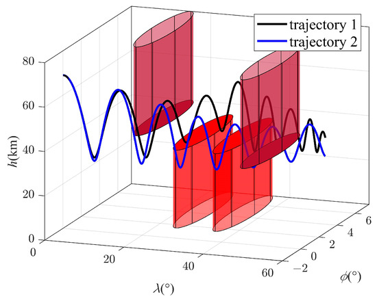
Figure 24.
Three-dimensional trajectory.
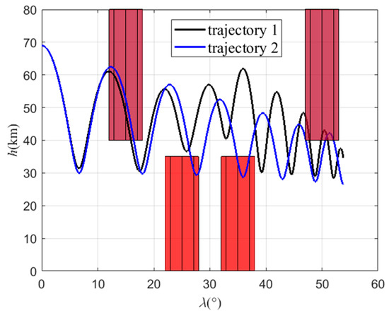
Figure 25.
Longitudinal trajectory.
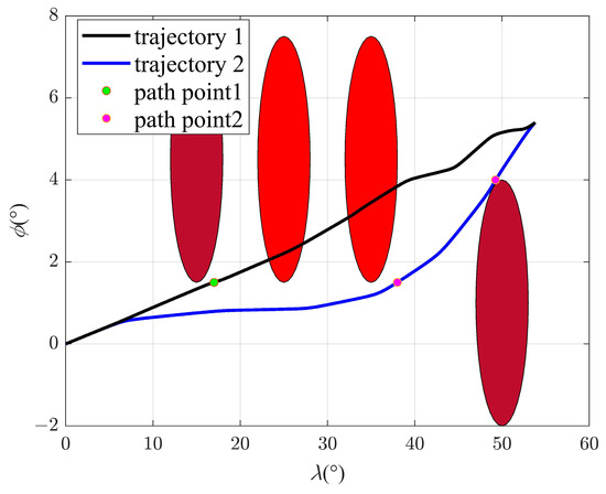
Figure 26.
Lateral trajectory.
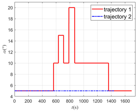
Figure 27.
Attack angle curve.
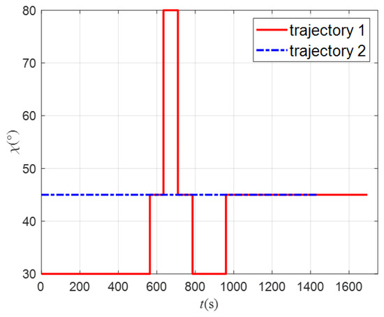
Figure 28.
Sweep angle curve.
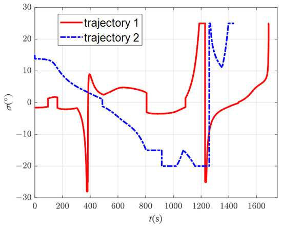
Figure 29.
Bank angle curve.
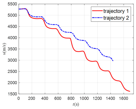
Figure 30.
Speed curve.
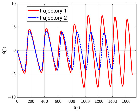
Figure 31.
Path angle curve.
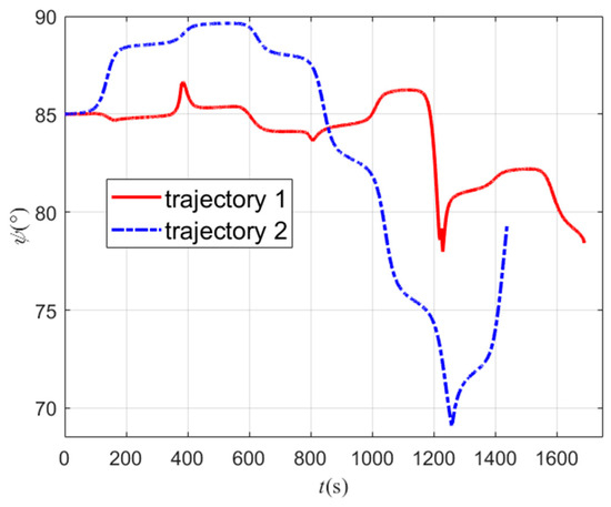
Figure 32.
Heading angle curve.
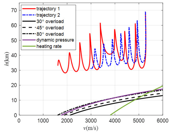
Figure 33.
H-V profile.
6. Conclusions
Aiming to address the safe trajectory planning problem of hypersonic morphing vehicles, this paper designed a trajectory planning algorithm using the predictor–corrector method, including a basic and an improved algorithm. In the basic algorithm, the angle of attack and sweep angle commands, flight path points, and bank angle commands are generated. The problem of aircraft trajectory planning is thereby solved. In the improved algorithm, MCRL and DNN are used to improve the predictor–corrector method, which reduces the planned turning angle and increases the final speed. The improved method produces a better trajectory by consuming more energy while ensuring safe flight and that the target is reached. The current work can be enriched in the future from the following aspects. The trajectory planning method in this paper is carried out under ideal conditions and without considering the influence of errors, such as sensor noise. At the same time, the trajectory planning method of the aircraft in this paper is only a feasible method, whereas the optimality of trajectory under various conditions is not guaranteed. In future research, trajectory planning methods considering errors and multiple constraints will be an important topic. This can improve the flight performance of the vehicle, allowing for accomplishing a wider variety of missions.
Author Contributions
Conceptualization, D.Y. and Q.X.; methodology, D.Y.; software, D.Y.; validation, D.Y.; formal analysis, D.Y.; investigation, D.Y.; resources, Q.X.; data curation, D.Y.; writing—original draft, D.Y.; writing—review and editing, D.Y. and Q.X.; visualization, D.Y.; supervision, Q.X.; project administration, Q.X.; funding acquisition, Q.X. All authors have read and agreed to the published version of the manuscript.
Funding
This research received no external funding.
Data Availability Statement
Not applicable.
Conflicts of Interest
The authors declare no conflict of interest.
References
- Bowman, J.; Plumley, R.; Dubois, J.; Wright, D. Mission Effectiveness Comparisons of Morphing and Non-Morphing Vehicles. In Proceedings of the 6th AIAA Aviation Technology, Integration and Operations Conference (ATIO), Wichita, KS, USA, 25–27 September 2006. [Google Scholar]
- Peng, W.; Yang, T.; Feng, Z.; Zhang, Q. Analysis of Morphing Modes of Hypersonic Morphing Aircraft and Multi-objective Trajectory Optimization. IEEE Access 2019, 7, 2244–2255. [Google Scholar] [CrossRef]
- Phoenix, A.A.; Maxwell, J.R.; Rogers, R.E. Mach 5–3.5 Morphing Wave-rider Accuracy and Aerodynamic Performance Evaluation. J. Aircr. 2019, 56, 2047–2061. [Google Scholar] [CrossRef]
- Sun, J.; Guan, Q.; Liu, Y.; Leng, J. Morphing aircraft based on smart materials and structures: A state-of-the-art review. J. Intell. Mater. Syst. Struct. 2016, 27, 2289–2312. [Google Scholar] [CrossRef]
- Burdette, D.A.; Kenway, G.K.; Martins, J. Aerostructural design optimization of a continuous morphing trailing edge aircraft for improved mission performance. In Proceedings of the 17th AIAA/ISSMO Multidisciplinary Analysis and Optimization Conference, Washington, DC, USA, 13–17 June 2016. [Google Scholar]
- Peng, W.; Feng, Z.; Yang, T.; Zhang, B. Trajectory multi-objective optimization of hypersonic morphing aircraft based on variable sweep wing. In Proceedings of the 2018 3rd International Conference on Control and Robotics Engineering (ICCRE), Nagoya, Japan, 20–23 April 2018. [Google Scholar]
- Yang, H.; Chao, T.; Wang, S. Multi-objective Trajectory Optimization for Hypersonic Telescopic Wing Morphing Aircraft Using a Hybrid MOEA/D. In Proceedings of the 2022 China Automation Congress (CAC), Xiamen, China, 25–27 November 2022. [Google Scholar]
- Wei, C.; Ju, X.; He, F.; Lu, B.G. Research on Non-stationary Control of Advanced Hypersonic Morphing Vehicles. In Proceedings of the 21st AIAA International Space Planes and Hypersonics Technologies Conference, Xiamen, China, 6–9 March 2017. [Google Scholar]
- Guo, J.; Wang, Y.; Liao, X.; Wang, C.; Qiao, J.; Teng, H. Attitude Control for Hypersonic Morphing Vehicles Based on Fixed-time Disturbance Observers. In Proceedings of the 2022 China Automation Congress (CAC), Xiamen, China, 25–27 November 2022. [Google Scholar]
- Yufei, W.; Changsheng, J.; Qingxian, W. Attitude tracking control for variable structure near space vehicles based on switched nonlinear systems. Chin. J. Aeronaut. 2013, 26, 186–193. [Google Scholar]
- Afsar Rayhan, M.; Muhammad, M.; Arifuzzaman, M.; Swarnaker, D. Morphing Aircraft Research and Development: A Review. In Proceedings of the International Aerospace Engineering Conference 2015, Vancouver, BC, Canada, 27–28 August 2015. [Google Scholar]
- Barbarino, S.; Bilgen, O.; Ajaj, R.M.; Friswell, M.I.; Inman, D.J. A review of morphing aircraft. J. Intell. Mater. Syst., Struct. 2011, 22, 823–877. [Google Scholar] [CrossRef]
- Rodriguez, A. Morphing aircraft technology survey. In Proceedings of the 45th AIAA Aerospace Sciences Meeting and Exhibit, Reno, NV, USA, 8–11 January 2007. [Google Scholar]
- Bae, J.-S.; Seigler, T.M.; Inman, D.J. Aerodynamic and static aeroelastic characteristics of a variable-span morphing wing. J. Aircraft 2005, 42, 528–534. [Google Scholar] [CrossRef]
- Weisshaar, T.A. Morphing aircraft systems: Historical perspectives and future challenges. J. Aircraft 2013, 50, 337–353. [Google Scholar] [CrossRef]
- Shaughnessy, J.D.; Pinckney, S.Z.; McMinn, J.D. Hypersonic Vehicle Simulation Model: Winged-Cone Configuration; NASA Langley Research Center Hampton: Hampton, VA, USA, 1990; pp. 1–140. [Google Scholar]
- Takama, Y. Practical wave-rider with outer wings for the improvement of low-speed aerodynamic performanc. In Proceedings of the 17th AIAA International Space Planes and Hypersonic Systems and Technologies Conference, San Francisco, CA, USA, 11–14 April 2011. [Google Scholar]
- Wingrove, R.C. Survey of Atmosphere Re-entry Guidance and Control Methods. AIAA J. 1963, 1, 2019–2029. [Google Scholar] [CrossRef]
- Mease, K.; Chen, D.; Tandon, S. A three-dimensional predictive entry guidance approach. In Proceedings of the AIAA Guidance, Navigation and Control Conference and Exhibit, Dever, CO, USA, 14–17 August 2000. [Google Scholar]
- Zhao, H.L.; Liu, H.W. A Predictor-corrector Smoothing Newton Method for Solving the Second-order Cone Complementarity. In Proceedings of the 2010 International Conference on Computational Aspects of Social Networks, Taiyuan, China, 26–28 September 2010. [Google Scholar]
- Wang, H.; Li, Q.; Ren, Z. Predictor-corrector entry guidance for high-lifting hypersonic vehicles. In Proceedings of the 35th Chinese Control Conference (CCC), Chengdu, China, 27 July 2016. [Google Scholar]
- Liu, S.; Liang, Z.; Li, Q.; Ren, Z. Predictor-corrector guidance for entry with terminal altitude constraint. In Proceedings of the 2016 35th Chinese Control Conference (CCC), Chengdu, China, 27 July 2016. [Google Scholar]
- Xu, M.; Liu, L.; Tang, G.; Chen, K. Quasi-equilibrium glide auto-adaptive entry guidance based on ideology of predictor-corrector. In Proceedings of the 5th International Conference on Recent Advances in Space Technologies—RAST2011, Istanbul, Turkey, 9–11 June 2011. [Google Scholar]
- Li, W.; Sun, S.; Shen, Z. An adaptive predictor-corrector entry guidance law based on online parameter estimation. In Proceedings of the 2016 IEEE Chinese Guidance, Navigation and Control Conference (CGNCC), Nanjing, China, 12–14 August 2016. [Google Scholar]
- Liang, Z.; Ren, Z.; Bai, C.; Xiong, Z. Hybrid reentry guidance based on reference-trajectory and predictor-corrector. In Proceedings of the 32nd Chinese Control Conference, Xi’an, China, 26–28 July 2013. [Google Scholar]
- McMahon, J.W.; Amato, D.; Kuettel, D.; Grace, M.J. Stochastic Predictor-Corrector Guidance. In Proceedings of the AIAA SCITECH 2022 Forum, San Diego, CA, USA, Virtual, 3–7 January 2022. [Google Scholar]
- Chi, H.; Zhou, M. Trajectory Planning for Hypersonic Vehicles with Reinforcement Learning. In Proceedings of the 2021 40th Chinese Control Conference (CCC), Shanghai, China, 26–28 July 2021. [Google Scholar]
- Shen, Z.; Yu, J.; Dong, X.; Ren, Z. Deep Neural Network-Based Penetration Trajectory Generation for Hypersonic Gliding Vehicles Encountering Two Interceptors. In Proceedings of the 2022 41st Chinese Control Conference (CCC), Hefei, China, 25–27 July 2022. [Google Scholar]
- Kai, Z.; Zhenyun, G. Neural predictor-corrector guidance based on optimized trajectory. In Proceedings of the 2014 IEEE Chinese Guidance, Navigation and Control Conference, Yantai, China, 8–10 August 2014. [Google Scholar]
- Lv, Y.; Hao, D.; Gao, Y.; Li, Y. Q-Learning Dynamic Path Planning for an HCV Avoiding Unknown Threatened Area. In Proceedings of the 2020 Chinese Automation Congress (CAC), Shanghai, China, 6–8 November 2020. [Google Scholar]
- Gaudet, B.; Drozd, K.; Furfaro, R. Adaptive Approach Phase Guidance for a Hypersonic Glider via Reinforcement Meta Learning. In Proceedings of the AIAA SCITECH 2022 Forum, San Diego, CA, USA, Virtual, 3–7 January 2022. [Google Scholar]
- Subramanian, J.; Mahajan, A. Renewal Monte Carlo: Renewal Theory-Based Reinforcement Learning. IRE Trans. Autom. Control 2020, 65, 3663–3670. [Google Scholar] [CrossRef]
- Peters, J.F.; Lockery, D.; Ramanna, S. Monte Carlo off-policy reinforcement learning: A rough set approach. In Proceedings of the Fifth International Conference on Hybrid Intelligent Systems (HIS’05), Rio de Janeiro, Brazil, 6–9 November 2005. [Google Scholar]
- Lipkis, R.; Lee, R.; Silbermann, J.; Young, T. Adaptive Stress Testing of Collision Avoidance Systems for Small UASs with Deep Reinforcement Learning. In Proceedings of the AIAA SCITECH 2022 Forum, San Diego, CA, USA, Virtual, 3–7 January 2022. [Google Scholar]
- Bhadoriya, A.S.; Darbha, S.; Rathinam, S.; Casbeer, D.; Rasmussen, S.J.; Manyam, S.G. Multi-Agent Assisted Shortest Path Planning using Monte Carlo Tree Search. In Proceedings of the AIAA SCITECH 2023 Forum, National Harbor, MD, USA, Online, 23–27 January 2023. [Google Scholar]
- Lu, P. Entry Guidance: A Unified Method. J. Guid. Control Dynam. 2014, 37, 713–728. [Google Scholar] [CrossRef]
- Han, P.; Shan, J. RLV’s re-entry trajectory optimization based on B-spline theory. In Proceedings of the 2011 International Conference on Electrical and Control Engineering, Yichang, China, 16–18 September 2011. [Google Scholar]
- Adsawinnawanawa, E.; Keeratipranon, N. The Sharing of Similar Knowledge on Monte Carlo Algorithm applies to Cryptocurrency Trading Problem. In Proceedings of the 2022 International Electrical Engineering Congress (iEECON), Khon Kaen, Thailand, 9–11 March 2022. [Google Scholar]
Disclaimer/Publisher’s Note: The statements, opinions and data contained in all publications are solely those of the individual author(s) and contributor(s) and not of MDPI and/or the editor(s). MDPI and/or the editor(s) disclaim responsibility for any injury to people or property resulting from any ideas, methods, instructions or products referred to in the content. |
© 2023 by the authors. Licensee MDPI, Basel, Switzerland. This article is an open access article distributed under the terms and conditions of the Creative Commons Attribution (CC BY) license (https://creativecommons.org/licenses/by/4.0/).