
Comparison of Actual and Time-Optimized Flight Trajectories in the Context of the In-Service Aircraft for a Global Observing System (IAGOS) Programme

 , , , and
Abstract
:1. Introduction
2. Data and Methodology
2.1. Problem to Solve and Simplifying Assumptions
2.2. Data
2.3. Reprojection
2.4. Cost Function
2.5. Gradient Descent
2.6. Zermelo Method
3. Results
3.1. Timings
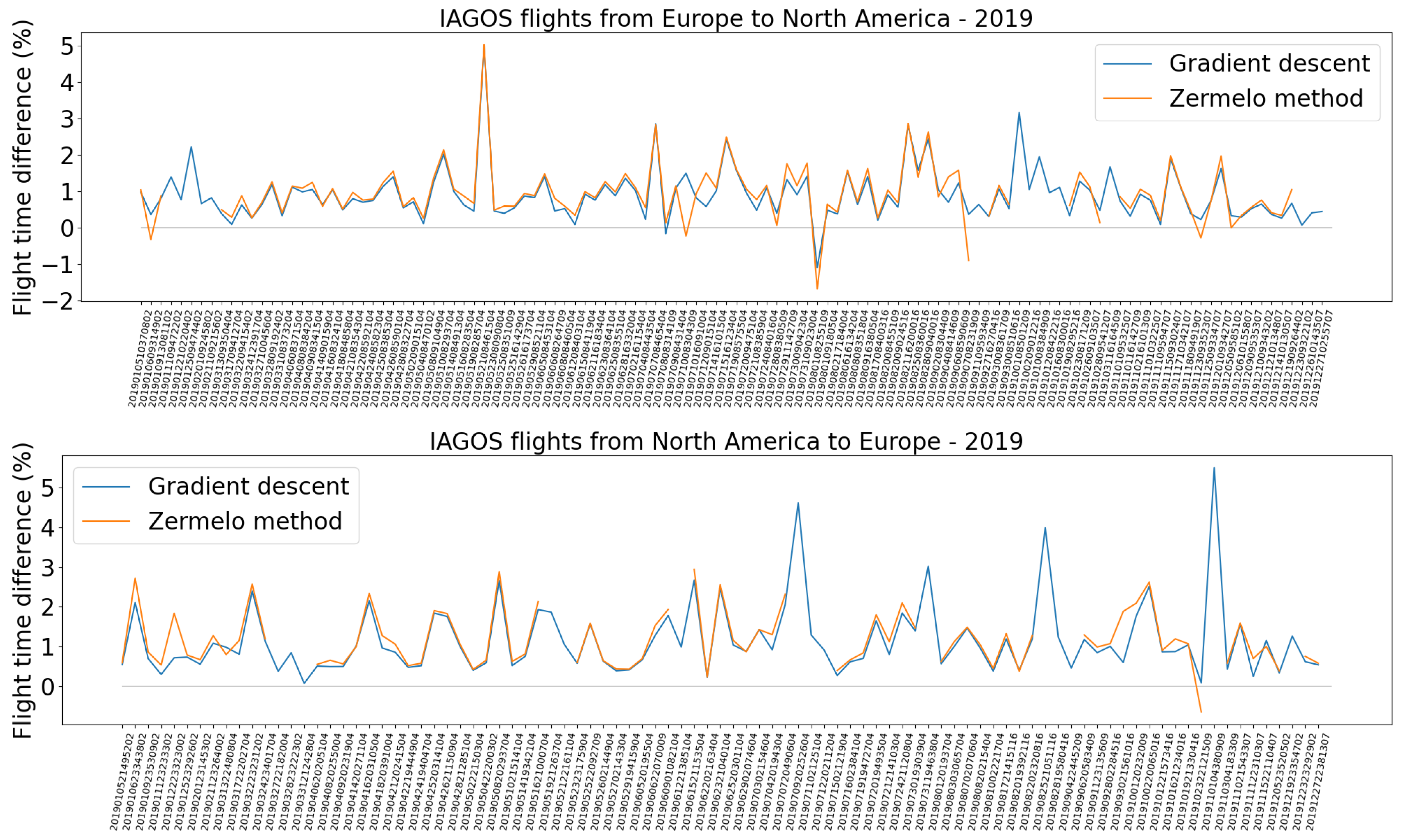
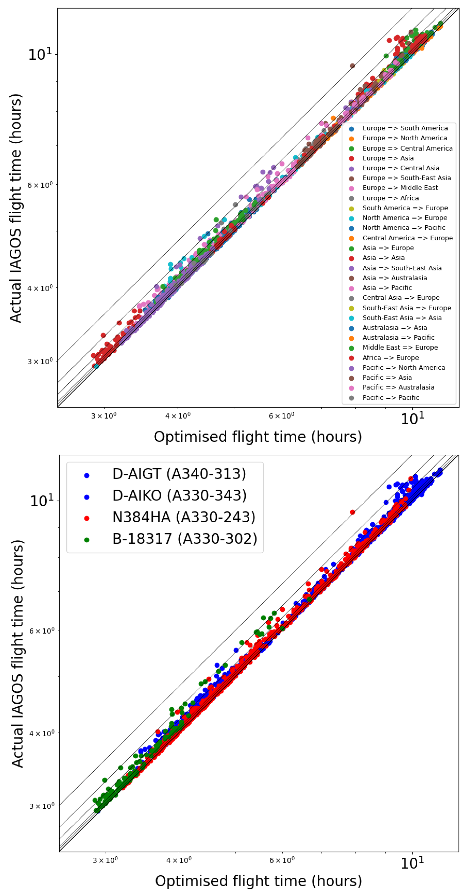
3.2. Statistics
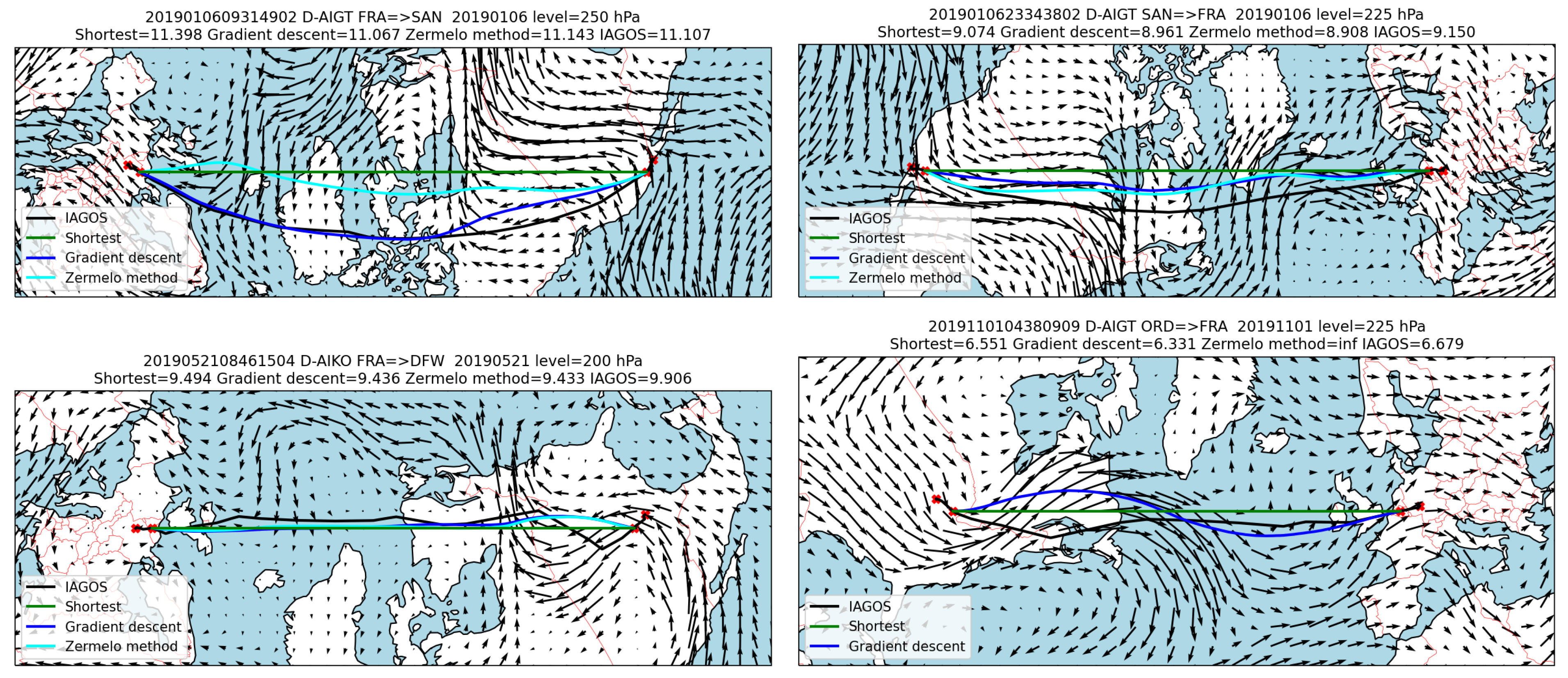
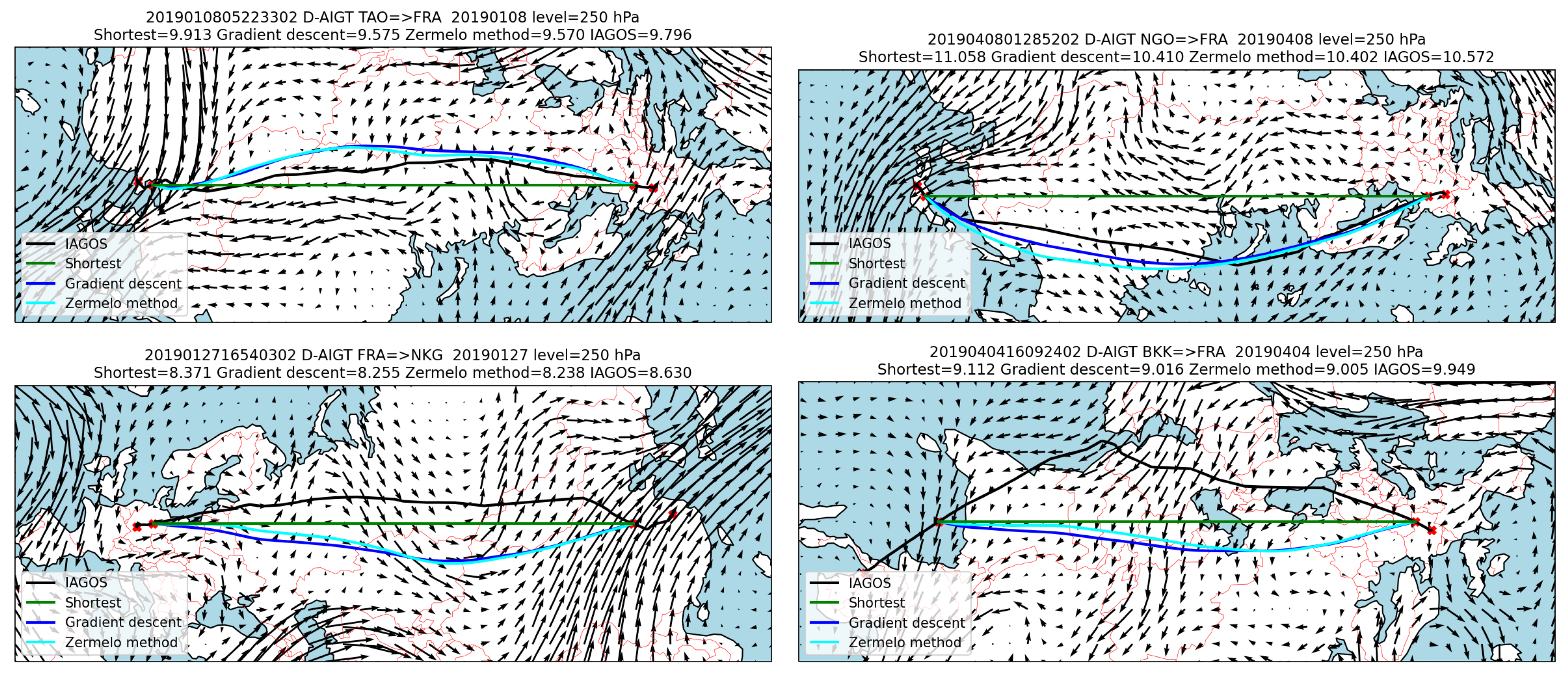
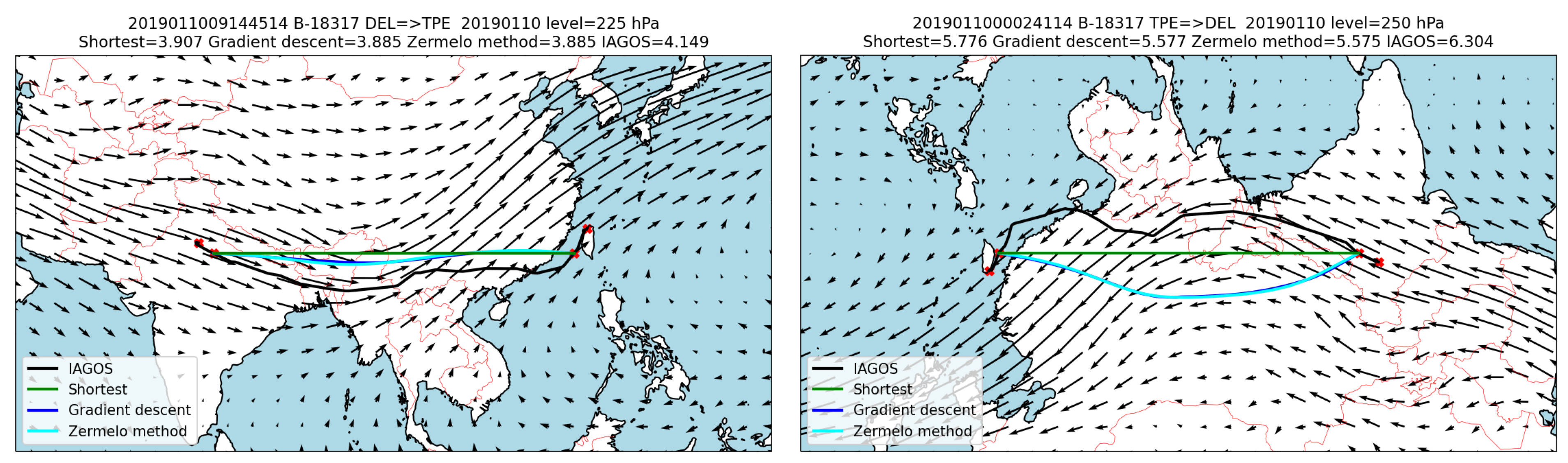
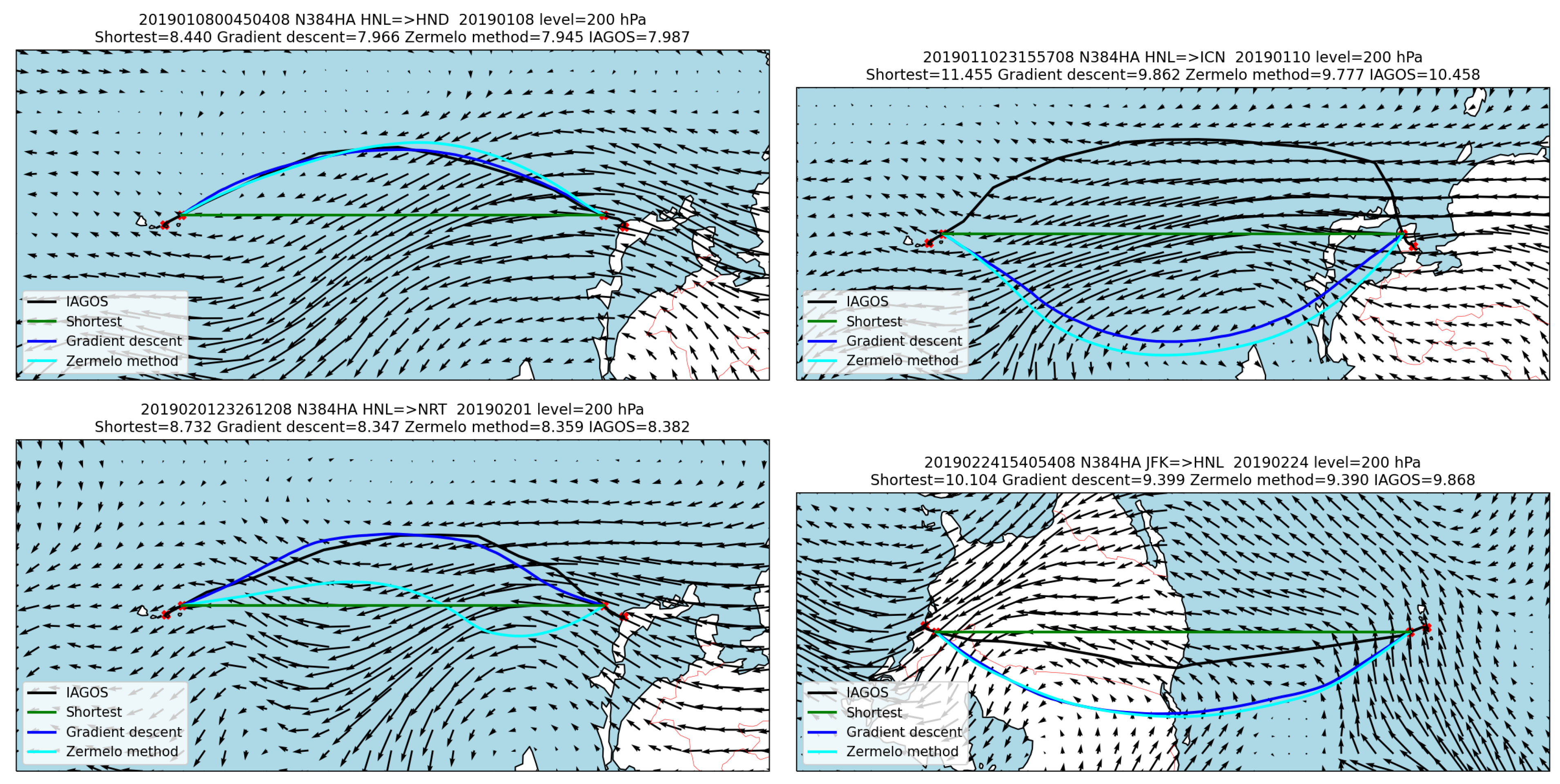
3.3. Examples of Time-Optimized Trajectories in Comparison to Actual Trajectories
4. Discussion and Conclusions
Supplementary Materials
Author Contributions
Funding
Informed Consent Statement
Data Availability Statement
Acknowledgments
Conflicts of Interest
References
- Dalmau Codina, R.; Melgosa Farrés, M.; Vilardaga Garcia-Cascón, S.; Prats Menéndez, X. A fast and flexible aircraft trajectory predictor and optimiser for ATM research applications. In Proceedings of the International Conference on Research in Air Transportation, Catalonia, Spain, 25–29 June 2018. [Google Scholar]
- Eurocontrol. Environmental Assessment: European ATM Network Fuel Inefficiency Study. Technical Report, Eurocontrol, 8 December 2020. Available online: https://www.eurocontrol.int/publication/environmental-assessment-european-atm-network-fuel-inefficiency-study (accessed on 22 August 2023).
- Wells, C.A.; Williams, P.D.; Nichols, N.K.; Kalise, D.; Poll, I. Reducing transatlantic flight emissions by fuel-optimised routing. Environ. Res. Lett. 2021, 16, 025002. [Google Scholar] [CrossRef]
- Liu, Y.; Hansen, M.; Ball, M.O.; Lovell, D.J. Causal analysis of flight en route inefficiency. Transp. Res. Part Methodol. 2021, 151, 91–115. [Google Scholar] [CrossRef]
- Prats, X.; Dalmau, R.; Barrado, C. Identifying the sources of flight inefficiency from historical aircraft trajectories. A set of distance- and fuel-based performance indicators for post-operational analysis. In Proceedings of the 13th USA/Europe Air Traffic Management Research and Development Seminar, Vienna, Austria, 17–21 June 2019. [Google Scholar]
- Kuljanin, J.; Pons-Prats, J.; Prats, X. Fuel-based flight inefficiency through the lens of different airlines and route characteristics, A post-operational analysis for one day of traffic at the ECAC area. In Proceedings of the 14th USA/Europe Air Traffic Management Research and Development Seminar, Virtual Event, 20–23 September 2021. [Google Scholar]
- Wells, C.; Kalise, D.; Nichols, N.; Poll, I.; Williams, P. The role of airspeed variability in fixed-time, fuel-optimal aircraft trajectory planning. Optim. Eng. 2023, 24, 1057–1087. [Google Scholar] [CrossRef]
- Wells, C.A.; Williams, P.D.; Nichols, N.K.; Kalise, D.; Poll, I. Minimising emissions from flights through realistic wind fields with varying aircraft weights. Transp. Res. Part Transp. Environ. 2023, 117, 103660. [Google Scholar] [CrossRef]
- Lee, D.; Fahey, D.; Skowron, A.; Allen, M.; Burkhardt, U.; Chen, Q.; Doherty, S.; Freeman, S.; Forster, P.; Fuglestvedt, J.; et al. The contribution of global aviation to anthropogenic climate forcing for 2000 to 2018. Atmos. Environ. 2021, 244, 117834. [Google Scholar] [CrossRef]
- Niklaß, M.; Dahlmann, K.; Grewe, V.; Maertens, S.; Plohr, M.; Scheelhaase, J.; Schwieger, J.; Brodmann, U.; Kurzböck, C.; Repmann, M.; et al. Integration of Non-CO2 Effects of Aviation in the EU ETS and under CORSIA, Final Report, Climate Change 00/2019. Technical Report, German Environment Agency. 2019. Available online: https://www.umweltbundesamt.de/publikationen/integration-of-non-co2-effects-of-aviation-in-the (accessed on 30 June 2023).
- EASA. Updated Analysis of the non-CO2 Climate Impacts of Aviation and Potential Policy Measures Pursuant to the EU Emissions Trading System Directive Article 30(4). Technical Report, EASA, August 2020. Available online: https://www.easa.europa.eu/en/document-library/research-reports/report-commission-european-parliament-and-council (accessed on 30 June 2023).
- Teoh, R.; Schumann, U.; Stettler, M. Beyond contrail avoidance: Efficacy of flight altitude changes to minimise contrail climate forcing. Aerospace 2020, 7, 121. [Google Scholar] [CrossRef]
- Teoh, R.; Schumann, U.; Gryspeerdt, E.; Shapiro, M.; Molloy, J.; Koudis, G.; Voigt, C.; Stettler, M.E.J. Aviation contrail climate effects in the North Atlantic from 2016 to 2021. Atmos. Chem. Phys. 2022, 22, 10919–10935. [Google Scholar] [CrossRef]
- Sridhar, B.; Ng, H.K.; Chen, N.Y. Aircraft trajectory optimization and contrails avoidance in the presence of winds. J. Guid. Control Dyn. 2011, 34, 1577–1584. [Google Scholar] [CrossRef]
- Lim, Y.; Gardi, A.; Sabatini, R. Modelling and evaluation of aircraft contrails for 4-dimensional trajectory optimisation. SAE Int. J. Aerosp. 2015, 8, 248–259. [Google Scholar] [CrossRef]
- Zou, B.; Buxi, G.; Hansen, M. Optimal 4-D aircraft trajectories in a contrail-sensitive environment. Netw. Spat. Econ. 2016, 16, 415–446. [Google Scholar] [CrossRef]
- Rosenow, J.; Fricke, H.; Luchkova, T.; Schultz, M. Minimizing contrail formation by rerouting around dynamic ice-supersaturated regions. Aeronaut. Aerosp. Open Access J. 2018, 2, 105–111. [Google Scholar] [CrossRef]
- Yin, F.; Grewe, V.; Frömming, C.; Yamashita, H. Impact on flight trajectory characteristics when avoiding the formation of persistent contrails for transatlantic flights. Transp. Res. Part Transp. Environ. 2018, 65, 466–484. [Google Scholar] [CrossRef]
- Irvine, E.A.; Hoskins, B.J.; Shine, K.P. A simple framework for assessing the trade-off between the climate impact of aviation carbon dioxide emissions and contrails for a single flight. Environ. Res. Lett. 2014, 9, 064021. [Google Scholar] [CrossRef]
- Grewe, V.; Matthes, S.; Frömming, C.; Brinkop, S.; Jöckel, P.; Gierens, K.; Champougny, T.; Fuglestvedt, J.; Haslerud, A.; Irvine, E.; et al. Feasibility of climate-optimized air traffic routing for trans-Atlantic flights. Environ. Res. Lett. 2017, 12, 034003. [Google Scholar] [CrossRef]
- Yin, F.; Grewe, V.; Castino, F.; Rao, P.; Matthes, S.; Dahlmann, K.; Dietmüller, S.; Frömming, C.; Yamashita, H.; Peter, P.; et al. Predicting the climate impact of aviation for en-route emissions: The algorithmic climate change function submodel ACCF 1.0 of EMAC 2.53. Geosci. Model Dev. 2023, 16, 3313–3334. [Google Scholar] [CrossRef]
- Zermelo, E. Über die Navigation in der Luft als Problem der Variationsrechnung. Jahresber. Der Dtsch.-Math.-Ver. 1930, 39, 44–48. [Google Scholar]
- Sawyer, J.S. Pressure-pattern flying. Weather 1948, 3, 290–294. [Google Scholar] [CrossRef]
- Lunnon, R.; Marklow, A. Optimization of time saving in navigation through an area of variable flow. J. Navig. 1992, 45, 384–399. [Google Scholar] [CrossRef]
- Irvine, E.A.; Shine, K.P.; Stringer, M.A. What are the implications of climate change for trans-Atlantic aircraft routing and flight time? Transp. Res. Part Transp. Environ. 2016, 47, 44–53. [Google Scholar] [CrossRef]
- Parzani, C.; Puechmorel, S. On a Hamilton-Jacobi-Bellman approach for coordinated optimal aircraft trajectories planning. Optim. Control Appl. Methods 2018, 39, 933–948. [Google Scholar] [CrossRef]
- Yamashita, H.; Grewe, V.; Jöckel, P.; Linke, F.; Schaefer, M.; Sasaki, D. Air traffic simulation in chemistry-climate model EMAC 2.41: AirTraf 1.0. Geophys. Mod. Dev. 2016, 9, 3363–3392. [Google Scholar] [CrossRef]
- Yamashita, H.; Yin, F.; Grewe, V.; Jöckel, P.; Matthes, S.; Kern, B.; Dahlmann, K.; Frömming, C. Newly developed aircraft routing options for air traffic simulation in the chemistry–climate model EMAC 2.53: AirTraf 2.0. Geophys. Mod. Dev. 2020, 13, 4869–4890. [Google Scholar] [CrossRef]
- Yamashita, H.; Yin, F.; Grewe, V.; Jöckel, P.; Matthes, S.; Kern, B.; Dahlmann, K.; Frömming, C. Analysis of aircraft routing strategies for North Atlantic flights by using AirTraf 2.0. Aerospace 2021, 8, 33. [Google Scholar] [CrossRef]
- Simorgh, A.; Soler, M.; González-Arribas, D.; Linke, F.; Lührs, B.; Meuser, M.M.; Dietmüller, S.; Matthes, S.; Yamashita, H.; Yin, F.; et al. Robust 4D climate-optimal flight planning in structured airspace using parallelized simulation on GPUs: ROOST V1.0. Geosci. Model Dev. 2023, 16, 3723–3748. [Google Scholar] [CrossRef]
- Petzold, A.; Thouret, V.; Gerbig, C.; Zahn, A.; Brenninkmeijer, C.A.M.; Gallagher, M.; Hermann, M.; Pontaud, M.; Ziereis, H.; Boulanger, D.; et al. Global-scale atmosphere monitoring by in-service aircraft—current achievements and future prospects of the European Research Infrastructure IAGOS. Tellus 2015, 67, 28452. [Google Scholar] [CrossRef]
- Williams, P.D. Transatlantic flight times and climate change. Environ. Res. Lett. 2016, 11, 024008. [Google Scholar] [CrossRef]
- Liu, K.; Zheng, Z.; Zou, B.; Hansen, M. Airborne flight time: A comparative analysis between the U.S. and China. J. Air Transp. Manag. 2023, 107, 102341. [Google Scholar] [CrossRef]
- Seymour, K.; Held, M.; Georges, G.; Boulouchos, K. Fuel estimation in air transportation: Modeling global fuel consumption for commercial aviation. Transp. Res. Part Transp. Environ. 2020, 88, 102528. [Google Scholar] [CrossRef]
- Poll, D.; Schumann, U. An estimation method for the fuel burn and other performance characteristics of civil transport aircraft in the cruise. Part 1: Fundamental quantities and governing relations for a general atmosphere. Aeronaut. J. 2021, 125, 257–295. [Google Scholar] [CrossRef]


| From | To | Year | Nb Flights | IAGOS/ Quickest | Quickest/ Shortest | Shortest/ No Wind | IAGOS/ No Wind |
|---|---|---|---|---|---|---|---|
| North America | Pacific | 2019 | 216 | 1.016 | 0.985 | 1.078 | 1.079 |
| Pacific | North America | 2019 | 215 | 1.015 | 0.988 | 0.940 | 0.942 |
| Europe | North America | 2019 | 118 | 1.009 | 0.972 | 1.066 | 1.046 |
| North America | Europe | 2019 | 93 | 1.011 | 0.975 | 0.949 | 0.936 |
| Europe | Africa | 2019 | 91 | 1.020 | 0.992 | 1.002 | 1.014 |
| Europe | Asia | 2019 | 89 | 1.041 | 0.984 | 0.957 | 0.981 |
| Europe | Middle East | 2019 | 86 | 1.039 | 0.993 | 0.959 | 0.989 |
| Africa | Europe | 2019 | 85 | 1.020 | 0.993 | 1.010 | 1.022 |
| Middle East | Europe | 2019 | 72 | 1.034 | 0.991 | 1.053 | 1.080 |
| Asia | Europe | 2019 | 68 | 1.030 | 0.983 | 1.059 | 1.073 |
| Asia | Pacific | 2019 | 65 | 1.026 | 0.983 | 0.897 | 0.904 |
| Pacific | Asia | 2019 | 65 | 1.025 | 0.963 | 1.162 | 1.148 |
| Asia | Asia | 2019 | 63 | 1.029 | 0.998 | 1.003 | 1.030 |
| Europe | South America | 2019 | 31 | 1.008 | 0.970 | 1.064 | 1.041 |
| Australasia | Pacific | 2019 | 26 | 1.011 | 0.994 | 0.979 | 0.984 |
| Pacific | Australasia | 2019 | 26 | 1.018 | 0.992 | 1.034 | 1.044 |
| South America | Europe | 2019 | 24 | 1.013 | 0.978 | 0.953 | 0.944 |
| Europe | Central Asia | 2019 | 16 | 1.016 | 0.993 | 0.938 | 0.947 |
| Central Asia | Europe | 2019 | 16 | 1.014 | 0.989 | 1.072 | 1.075 |
| South-East Asia | Asia | 2019 | 12 | 1.081 | 0.991 | 0.896 | 0.960 |
| Europe | Central America | 2019 | 11 | 1.015 | 0.964 | 1.089 | 1.065 |
| Asia | South-East Asia | 2019 | 11 | 1.096 | 0.979 | 1.181 | 1.267 |
| Asia | Australasia | 2019 | 11 | 1.026 | 0.998 | 1.021 | 1.045 |
| Australasia | Asia | 2019 | 11 | 1.035 | 0.998 | 0.984 | 1.015 |
| Pacific | Pacific | 2019 | 10 | 1.011 | 0.995 | 1.008 | 1.014 |
| Central America | Europe | 2019 | 6 | 1.020 | 0.981 | 0.926 | 0.927 |
| Europe | South-East Asia | 2019 | 3 | 1.055 | 0.994 | 0.949 | 0.996 |
| South-East Asia | Europe | 2019 | 1 | 1.028 | 0.986 | 1.067 | 1.082 |
Disclaimer/Publisher’s Note: The statements, opinions and data contained in all publications are solely those of the individual author(s) and contributor(s) and not of MDPI and/or the editor(s). MDPI and/or the editor(s) disclaim responsibility for any injury to people or property resulting from any ideas, methods, instructions or products referred to in the content. |
© 2023 by the authors. Licensee MDPI, Basel, Switzerland. This article is an open access article distributed under the terms and conditions of the Creative Commons Attribution (CC BY) license (https://creativecommons.org/licenses/by/4.0/).
Share and Cite
Boucher, O.; Bellouin, N.; Clark, H.; Gryspeerdt, E.; Karadayi, J. Comparison of Actual and Time-Optimized Flight Trajectories in the Context of the In-Service Aircraft for a Global Observing System (IAGOS) Programme. Aerospace 2023, 10, 744. https://doi.org/10.3390/aerospace10090744
Boucher O, Bellouin N, Clark H, Gryspeerdt E, Karadayi J. Comparison of Actual and Time-Optimized Flight Trajectories in the Context of the In-Service Aircraft for a Global Observing System (IAGOS) Programme. Aerospace. 2023; 10(9):744. https://doi.org/10.3390/aerospace10090744
Chicago/Turabian StyleBoucher, Olivier, Nicolas Bellouin, Hannah Clark, Edward Gryspeerdt, and Julien Karadayi. 2023. "Comparison of Actual and Time-Optimized Flight Trajectories in the Context of the In-Service Aircraft for a Global Observing System (IAGOS) Programme" Aerospace 10, no. 9: 744. https://doi.org/10.3390/aerospace10090744
APA StyleBoucher, O., Bellouin, N., Clark, H., Gryspeerdt, E., & Karadayi, J. (2023). Comparison of Actual and Time-Optimized Flight Trajectories in the Context of the In-Service Aircraft for a Global Observing System (IAGOS) Programme. Aerospace, 10(9), 744. https://doi.org/10.3390/aerospace10090744