Article

Ice Accretion: Image Post-Processing Measurement Techniques for 2D Ice Shapes

1
Aero-Thermo-Mechanics Department, Faculty of Applied Sciences, Universitè Libre de Bruxelles, 1050 Brussels, Belgium
2
Environmental and Applied Fluid Dynamics Department, von Karman Institute for Fluid Dynamics, 1640 Rhode-Saint-Genèse, Belgium
3
UAV Icing Lab, Department of Engineering Cybernetics, Norwegian University of Science and Technology, 7491 Trondheim, Norway
4
UBIQ Aerospace, 7011 Trondheim, Norway
*
Authors to whom correspondence should be addressed.
Aerospace 2023, 10(5), 451; https://doi.org/10.3390/aerospace10050451
Submission received: 10 March 2023 / Revised: 24 April 2023 / Accepted: 8 May 2023 / Published: 13 May 2023
(This article belongs to the Special Issue Deicing and Anti-Icing of Aircraft (Volume III))

Abstract

:
Ice accretion poses substantial safety hazards for the manned and unmanned aviation industries. Its study is essential for icing events risk assessment and for the development of efficient ice protection systems. The existing ice accretion measurement techniques—casting, molding, and laser-scanning—are time-consuming, sometimes cumbersome to use, and highly expensive, while hand tracing is inexpensive, but has lower accuracy and time-consuming post-processing. This work presents two low-cost, fast, and easy-to-use measurement techniques for 2D ice accretion profiles. Both employ algorithms of automatic ice shape detection, one based on unmediated image-processing, another based on the processing of manual ice tracings. The techniques are applied to ice accretion experiments conducted in an icing wind tunnel at low Reynolds numbers, and their results are validated against ice thickness caliper measurements. A comparison of the results shows that both techniques accurately measure the leading-edge ice thickness and the 2D shape of the ice accretion profiles. One technique is faster, with higher measurement accuracy, but produces interrupted-line 2D ice profiles and requires good lighting conditions, while the other generates continuous-line 2D profiles and has no application restriction, but it is slower, with lower accuracy. A discussion is conducted, aiming to help one determine the best applications for each ice accretion measurement technique presented.

1. Introduction

Aircraft icing is an important safety hazard which has been studied since the 1920s [1] as it causes rapid performance degradation and malfunction of the flight instruments [2,3,4]. The first icing research analyzed the effects of ice accretion over the wings [5], and the importance of ice accretion studies remains relevant today [6,7,8]. Based on the ice shape, scientists and engineers evaluate the impact of icing on aerodynamic surfaces such as wings [5,9,10,11], propellers [12,13,14], and engine inlets [15,16,17]. These evaluations of the ice accretion impact are used in risk assessment for icing events, the development of new aviation regulations, and the research and development of ice mitigation techniques [18,19,20]. The aerodynamic penalties induced by different ice accretion regimes are studied both experimentally, in conventional wind tunnel tests with artificial ice shapes, as well as numerically, by means of simulations [21]. For both research methods, ice accretion measurements are critical for an accurate outcome. Over time, multiple ice accretion measurement methods were developed; all brought more knowledge about ice accretion physics, and all had their advantages and drawbacks.
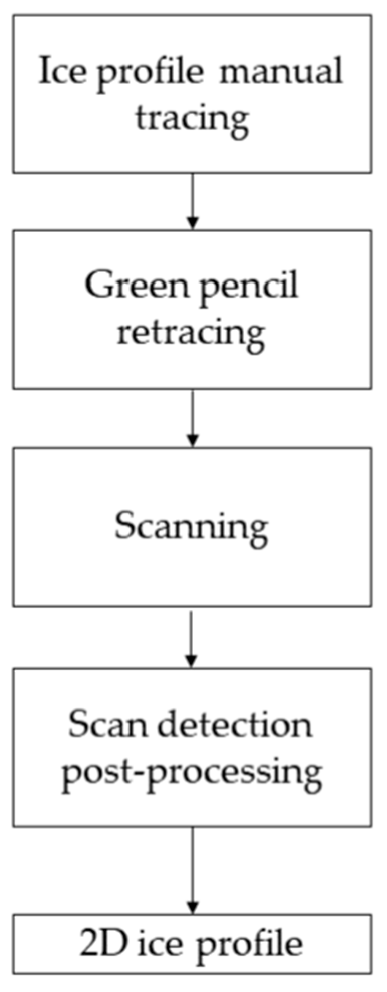
The first ice accretion measurement method was the manual tracing of ice shapes, which was also the most common technique in the past [22,23,24]. It is an inexpensive technique, in which only paper, a pencil, and a metal support are required, but the ice shape drawing process can be long and have a dampening effect on small ice surface features, and the manual digitalization post-processing is cumbersome.
Following this, complex 3D ice accretion measurement techniques were developed. First, molding and casting techniques were used to capture the ice accretion features and to produce artificial ice shapes from plasters and epoxy [25,26]. Ice profilometry was conducted on cast models. Most molding materials were temperature-dependent—thus, they affected the ice shape, producing damped or deformed ice molds. The casting formation process usually involved entraining air bubbles during the mixing and pouring phases, which generated brittle and deformed ice shapes [25].
Further, photogrammetry techniques were used to obtain 3D ice profiles [9,27]. The ice was photographed from multiple angles, and the shape was reconstructed using specialized software. Although it has increased accuracy and reduced cost compared to previous techniques, for cases of transparent ice (glaze accretion), a paint or powder layer must be added in order to avoid light reflections and refractions that would produce anomalies in the ice shape. These additional layers dampen some of the ice surface features and significantly increase the testing time because they require time to be deposed and to dry completely in order to obtain high-fidelity ice shapes [9].
Another technique successfully applied for measuring ice accretion profiles is the structured light technique [28,29,30], which relies on actively projecting a known light pattern on an object and extracting the 3D surface shape from images captured from one or more points of view. Being based on image correlation and the computation of displacement vectors between points of the projected grid, its results are spatial averages within a surface region. Thus, it has reduced accuracy in regions with steep ice thickness gradients. For accurate results, a parametric study on set-up alignment, grid projection resolution, and post-processing parameters must be performed before testing—a complex and time-consuming process.
More advanced laser-scanner techniques were developed and employed in the latest years. The laser-scanners have a high resolution and high accuracy and can generate both 3D and 2D ice profiles [31,32]. However, as with the photogrammetry, a layer of opaque painting must be sprayed on the ice before measuring. In addition, their high price (which usually varies between 50,000 to 100,000 euros) makes the technique cost-prohibitive for many research groups.
Expensive ice accretion methods are suitable for well-established icing facilities which focus on commercial and manned aviation. However, the developing fields of icing studies for different applications such as the unmanned aviation sector and wind turbine energy production have difficulties accessing these types of techniques. The icing research in these fields is seeing rapid growth, but it is still far from being fully established. This makes several advanced ice accretion measurement techniques cost-prohibitive. Especially for unmanned aerial vehicles (UAVs), for which icing impacts their operational range [33], this measurement capability is critical. As a result of the UAVs’ reduced size and flight at lower Reynolds numbers [34,35] compared to manned aviation, new ice accretion studies must be conducted for their specific flight conditions.
Therefore, in order to support the development of the UAV icing research field, inexpensive ice accretion measurement methods must be developed. Ideally, these new methods would employ equipment that is easily accessible to any research group, would be time-efficient (which would reduce the general testing costs), and could be used both inside an icing wind tunnel facility and in field missions. Given the nature of the testing environments, the most important features of the new techniques are to be both low-cost and easy-to-use. Especially for unmanned aviation, this would accelerate the development of ice protection systems and the validation of numerical simulation tools, accelerating the result of UAVs obtaining all-weather flying capabilities.
Looking at possible inexpensive solutions, measurement techniques based on image processing algorithms are used in many fields [36,37], from the research of physical phenomena [38,39,40,41], of environmental events [42,43,44], or medical research [45,46,47] to the assessment of industrial faults [48,49,50]. These types of algorithms provide non-invasive measurement capabilities, efficient ways to process big amounts of data, are cost-efficient, offer improved and reliable detection accuracy, and significantly reduce human error.
Therefore, this work proposes two different measurement techniques for 2D ice shapes based on image-processing algorithms. These were developed in order to offer more efficient and automatized alternatives to the time-consuming digitalization of hand drawings and low-cost alternatives to the 2D profiles obtained with the laser scanner technique. The algorithms are described in Section 2. Their capabilities were tested on ice accretion measurements over UAV wings. The tests were conducted in the icing wind tunnel of the VTT Technical Research Center of Finland over a wide temperature range, a process which generated the main ice accretion types: rime, mixed, and glaze. The models were validated against caliper measurements for pointwise ice thickness measurements on the leading edge, and for the generated 2D ice shapes, a comparison was performed between the 2D profiles obtained with each technique and is presented in Section 3. An additional algorithm was developed to convert the 2D ice profile into 1D ice thickness displayed over the chord length. This algorithm facilitates the use of thickness data at each airfoil coordinate and the comparison between the two image-processing techniques. Finally, each method’s capabilities are discussed together with their most suitable application and possible sources of error in Section 4. Based on the techniques’ comparison, conclusions are drawn, and improvements are suggested.

2. Methodology

The ice accretion experiments analyzed in this work were performed in the icing wind tunnel of the VTT Technical Research Center of Finland over the course of two experimental campaigns in 2019 and 2020. Based on this dataset, two algorithms to extract the ice thickness information in 2D profiles were developed and are presented in this section: one picture based (image-processing), another hand-drawing based (scan detection). A further post-processing algorithm was developed to convert the 2D profiles into 1D ice thickness profiles with pointwise measurements along the chord.

2.1. Experimental Method and Testing Conditions

The dataset was obtained by employing the testing facility [51] illustrated in Figure 1, which is an open-circuit icing wind tunnel (IWT) placed in a large climate chamber [52]. It can generate experimental testing conditions of up to 50 m/s wind speed for temperatures varying between −25 °C to 30 °C. Its 0.7 m × 0.7 m × 1 m test section is fed with water droplets generated by an array of 3 × 3 nozzles which can produce liquid water contents (LWC) between 0.1 to 1.0 g/m3 and median droplet volume diameters (MVD) in the range of 12 to 30 µm.
For these tests, the airfoil model was placed at the end of the test section, with only the leading edge being fitted inside of it, in order to ensure a 2D airflow and to avoid any edge effects influencing the trajectory of the water droplets. As these experimental campaigns were designed for multiple studies, three rectangular wing models were tested in the ice accretion campaign. All three are specific to low-Reynolds-number regimes: two RG-15 airfoils, which are specifically designed for UAV wings and airplane models, and an SD8020 symmetric airfoil, which is designed for tail surfaces. The models were provided by UBIQ Aerospace. They were manufactured from fiber-reinforced epoxy and their dimensions are presented in Table 1.
The experimental conditions were chosen in order to generate the three ice accretion regimes (glaze, mixed, and rime) that could be encountered during UAV operations [6,53]. Table 2 presents the test matrix. The LWC was measured before the tests using the rotating cylinder method. The rotating cylinder was placed at the end of the test section in the same position where the leading edge of the wing models was placed during the experiments.
The testing procedure begins with running the icing wind tunnel for the chosen ice accretion time. Afterward, the airfoil is carefully removed from the testing position to allow for better access, and the resulting iced leading edge is photo-documented in order to capture the ice’s physical properties, such as opacity, irregularities, and specific ice formations. Exemplary frontal images of the leading-edge ice formations for glaze, mixed, and rime regimes are illustrated in Figure 2a,c,e together with their corresponding side views in Figure 2b,d,f. Later, these are further used to extract the 2D ice profiles with one of the developed measurement techniques.
The process of obtaining these side views and the ice accretion measurements starts with the generation of ice cuts in several spanwise positions (which were previously marked on the wing),as the ice shape might slightly vary in this direction [9]. For this, a metallic plate with the negative shape of the airfoil’s leading edge is heated by submerging it in warm water. The warm plate is carefully placed on the pre-marked positions (Figure 3a) where it locally melts the ice and forms the ice cuts (shown in Figure 3b). Afterward, an electronic caliper is used to measure the thickness of ice by placing it in the ice cuts in the normal direction to the leading edge’s surface (Figure 3c).
Next, for the 2D ice profiles, two types of measurements are taken. First, a calibration paper is mounted on the metallic plate, and this ensemble is aligned with the airfoil’s leading edge in the formed cuts. Then, a pencil is used to manually trace the ice profile, as shown in Figure 3d. The tracing is conducted slowly and carefully so as not to damage the ice shape. Moreover, ice tracing is completed first in order to ensure that, regardless of any possible damage done to the ice, both methods will measure the same ice profile. These drawings are further processed with the scan detection method, which is described in Section 2.3.
Second, in order to obtain the side view images presented in Figure 2b,d,f, the metallic plate is used to double the cuts and to generate thin ice segments that remain attached to the wing, while the rest of the ice is removed using the heated plate. This procedure ensures a clean optical path between the camera and the ice segment. Next, a new calibration paper is mounted, and the plate–paper ensemble is used as the background and the alignment check for the image and camera’s perpendicularity, respectively. The camera is placed as perpendicularly to the ice segment as possible, and the network of cross signs on the calibration paper is used to check its position—the distance between two crosses should be equal in all regions of the image. This calibration distance will later be used by both measurement techniques to compute the magnification factor and apply scaling to retrieve the thickness of the ice from the 2D profiles. The generated images (Figure 2b,d,f) are further employed in the image processing method to retrieve the 2D ice profiles, as described in Section 2.1.
Finally, after obtaining the 2D profiles with both methods, the results are validated against the caliper measurements. Given that, for certain applications (such as a fast icing severity assessment or ice mass accumulation), a 1D ice thickness profile along the airfoil could be more efficient, a 1D thickness algorithm was developed and applied to convert the 2D profiles, and it is presented in Section 2.4.
The experimental validation and all of the results are presented in Section 3, and the techniques are compared and discussed in Section 4, where best practices to maximize their accuracy are suggested. The work is concluded in Section 5.

2.2. Image-Processing Ice Edge Detection Method

Given the technique’s advantages, an image processing algorithm was developed for automatic ice edge detection from the experimental side views in order to generate 2D ice profiles and fast and accurate ice thickness measurements. The goal was to obtain a low-cost measurement technique that reduces the data acquisition time and error compared to the manual tracing method and has a fast, efficient, and reliable post-processing method. The algorithm was developed in MATLAB, version R2018b, and it is based on directional image analysis with a grayscale gradient identification, similar to LeDaR [38] (level detection and recording), followed by image binarization and morphological operations to filter out the eventual outliers and to generate the final ice edge profile. The detection process can be adapted to each case by employing several adjustable parameters—which, for good-quality images (with minimal light reflections or shadows), are constant for each ice accretion regime. The algorithm performs edge detection for all ice accretion regimes. When necessary, an extra step—prediction of the leading edge reference point—can be enabled, such as in cases of opaque ice where the calibration paper is not visible through the ice (e.g., rime and mixed accretion). The main steps of the image processing ice edge detection method are illustrated in Figure 4.

2.2.1. Image Correction Pre-Processing

Before applying the post-processing algorithm, a quality check of the images and a pre-processing step are necessary. The camera should be placed perpendicular to the ice shape and the calibration plate, with the calibration signs visible and equidistant in all of the image regions. The light reflections and shadows should be minimized. Following data acquisition, the images are pre-processed with the Adobe Lightroom Classic software, wherein the Lens Correction feature is used to correct the optical distortion produced by the camera’s lenses. Afterward, post-processing is applied. The IP algorithm steps are illustrated on a glaze ice test case in Figure 5.

2.2.2. Edge Detection Algorithm

In the experimental image (Figure 5), the user signals two calibration signs and inputs their on-paper distance in millimeters. With this information, the algorithm computes the magnification factor in pixels/mm, which will later be used to scale the detected ice profile.
Next, the image is cropped to the region of interest (ROI), as is shown in Figure 6a, in which the user signals the leading-edge reference point (which is visible in this case) while the algorithm illustrates it (the magenta cross) and retains its position.
Afterward, automatic detection begins with the conversion of the image from RGB to grayscale in order to allow for one intensity gradient check. The resulting image is treated as a matrix, and on its every row and column, unidimensional intensity gradients are computed. In each profile, the algorithm searches for the local peak of the intensity gradient for a specified directional criterion (‘first’ for the vertical profiles, the columns, and ‘first’/’last’ for the horizontal ones, the rows). The search is conducted directionally because, generally, these local peaks of the intensity gradient correspond to the ice edges. However, in order to account for possible optical imperfections (shadows/reflections) and changes in the optical aspect of ice between accretion regimes, computational coefficients based on the allowed standard deviation of the intensity are imposed for each type of directional search. This varies the size of the peak of the intensity gradient considered for detection. For each directional search, the algorithm detects the local maximum gradient in each row/column following the criteria imposed and retains its position, generating a raw ice profile detection (Figure 6b).
With these identified positions, a binary matrix is formed (Figure 6c). Several methods of morphological filtering (removal of isolated pixels or clusters of pixels smaller than a certain threshold) are applied in order to obtain the final ice profile (Figure 6d).
As a verification step, the profile is plotted over the original cropped image (Figure 6e). If the result is satisfactory, then the reference point is replotted, and the user can continue with signaling the airfoil profile with at least 8 points (the black + signs in Figure 6f). From these points, the algorithm will apply a spline interpolation to generate the airfoil profile (the interrupted red line in Figure 6f).
Finally, the scaling is applied, and the ice profile is retrieved in millimeters. In order to compute the leading-edge ice thickness, the ice profile is interpolated to find the thickness value corresponding to the LE reference point (yLE = 0). To check for accuracy, this value is compared to the caliper measurement. As the detected ice profile might have gaps due to the filters applied, a profile reconstruction step based on a built-in MATLAB interpolation function is used to generate a continuous-line ice profile (green line in Figure 5b). However, because losses of accuracy might occur in this step, the use of the reconstructed profile is advised only in applications where an approximate ice shape is suitable. For cases with low-quality images (those with significant shadows or light reflections; see Section 3.2) which generate large gaps in the detected ice profile, the reconstruction step should be avoided. In these cases, the interpolation method will generate faulty profiles (see Appendix A, Figure A1). To include the difficult cases in the analysis of the IP technique, only the detected ice profiles are presented in this work. Good practices for maximizing the accuracy and the completeness of the detected profiles using the IP method are presented in Section 4.
The process is identical in the case of rime ice accretion (Figure 7), which is presented below (Figure 8). What differs in this case are the optical properties of the ice, which make the direct signaling of the LE reference point by the user impossible. In this case, an additional step is required before cropping the image: the estimation of the reference point position. This is achieved based on the nearby calibration points, using their position and the pixel distance defined in the magnification factor computation. The final result is shown in Figure 7b. As verification, the predicted LE cross should form a straight horizontal line with the other two, as seen in Figure 7b.
In this case, it can be seen that, although the predicted LE reference falls on the same line with the lateral calibration signs, the reference point is higher than the airfoil’s LE (visible in Figure 8a and the comparison between Figure 8e,f). This is a case in which the calibration paper is slightly misaligned, which generates a very similar percentual error with both techniques when compared to the caliper measurement. Therefore, this step can be useful also for identifying misalignment errors.
After the computation of the LE reference point, the process follows the usual steps, as described in Figure 8. The final result for this rime ice accretion case is shown in Figure 9.

2.2.3. Image-Processing Ice Edge Detection Technique’s Uncertainty

The uncertainty of the technique is assumed to be dependent on the uncertainty of the ice edge detection in the pixel space, the uncertainty of the magnification factor computation—which is applied to obtain physical thickness units—and the alignment uncertainty of the LE reference point (which can be higher in cases of opaque ice, i.e., rime and mixed accretion). Of these sources of error, the calibration paper misalignment is the most concerning, and it should be given special attention during the experiments. The other two uncertainties are random and very small (they are at a pixel level). As the camera perpendicularity is checked with the calibration paper and the images are corrected for optical distortion, the uncertainty of the camera alignment is neglected.

2.3. Manual Drawings Scan Detection Method

The idea behind the scan detection method is to take a manual tracing of the ice shape, scan the tracing, and use an algorithm to digitize the ice shape. Its main process steps are illustrated in Figure 10. It should be noted that the scan detection method is not completely novel but is an improvement to manual tracings because it uses an automatized post-processing algorithm.

2.3.1. Scan Pre-Processing

The first step is to take a manual tracing of the ice shape. Manual tracing was the most common method used to obtain information about ice shapes in the past [22,23,24]. First, a clean cut is made in the ice using a heated aluminum plate with a cut-out of the airfoil shape. Then, a paper template is fixed on this aluminum plate and put in the gap in the ice. The ice is traced manually on the paper template using a pencil. An exemplary resulting tracing is shown in Figure 11b. The paper sheet used for this study had a header to insert run-specific information like the run number, the conditions, and the position of the tracing on the wing in a spanwise direction. This information helps one to connect the different tracings with the runs and spanwise positions. Another feature of the paper sheets was that eight red crosses were placed with some distance between them and the airfoil (see Figure 11a). Adding these crosses allows for scaling the results to the original size in the end, independent of possible scaling issues while scanning the tracing or conducting post-processing on the tracing.
Instead of scanning the manual tracing directly, the ice shapes are first marked with a green pencil, as can be seen in Figure 12a. Coloring the ice shape offers three advantages compared to using the original tracing. First, it enables color detection in the detection algorithm, since nothing else on the paper should be green. Otherwise, it could be more complicated to distinguish the ice shape tracing from the other features on the paper. Second, coloring the ice shape is also a preliminary step in post-processing the manual tracing. This is necessary because the cold temperatures inside the cold room and the small features of the ice shapes make it difficult to cleanly trace the ice shape. Instead, multiple attempts might be required in order to trace every feature of an ice shape. Thus, by marking the tracings a second time, the correct lines can be traced, resulting in a cleaner ice shape tracing. Third, the detection algorithm used to digitize the ice tracing requires a connected line. Due to the difficulties mentioned before, the original tracing might not always be connected. By tracing the ice shape again, it can be ensured that the ice shape consists of a connected line. Since mistakes can also be made while tracing the manual drawings, this step was typically not performed on the original sheet of paper but rather on a copy. This allows for the storage of the original sheet of paper for future purposes.

2.3.2. Scan Detection Algorithm

After the ice shape is marked with a green pencil, the paper template must be scanned. The scan detection algorithm was coded in MATLAB, version 2021b. After the scan is selected, the tracing is rotated using the crosses as orientation. This ensures that any potential rotation of the paper, for example while scanning, is removed.
In the next step, the algorithm detects the green tracing of the ice shape. First, the RGB values of the image are converted into the CIE 1976 L*a*b* value system. Then, only pixels that are within certain thresholds for all three channels are kept. These thresholds must be tuned for the specific color of the pencil and might also vary for green-colored pencils from different manufacturers. Since there can be small mistakes in the green tracing, only the longest connected green line is kept, and this line is assumed to be the real ice shape. Finally, the size of the ice shape is scaled according to the measured distances between the crosses.
The result of the algorithm is a two-dimensional point cloud of the points that make up the ice shape. The agreement between the original tracing and the detected shape is very good, as can be seen in Figure 12b.

2.3.3. Manual Drawing Scan Detection Technique’s Uncertainty

The first challenge related to manual tracings is the melting of a thin layer of ice behind the area of interest. Since heat will be conducted in all directions, the traced ice shape is likely to be slightly changed. Another problem can occur at “warm” temperatures like −2 °C. When melting the ice, the interface between the surface and the ice might also be slightly melted. This decreases the adhesive forces between the surface and the ice, and the ice starts sliding off the wing easily.
Another set of challenges and uncertainties is related to the manual tracing of the ice shape. First, the template should be perfectly aligned with the airfoil in order to capture the ice shape. Otherwise, the traced ice shape will be slightly rotated compared to the real ice shape. Second, especially for ice shapes with many small features, it is difficult to trace the ice shape with high accuracy. Additionally, small features of the ice shape will sometimes be broken off while tracing the ice shape.
The processing of the ice tracing by copying it, marking it with a green pencil, and then scanning it also has the potential for some errors. First, the resolution of the copying and scanning will limit the resolution of the final results. However, the resolution of modern devices should be good enough to only introduce negligible errors. Since the marking with the green pencil is achieved manually as well, some differences between the marked tracing and the original tracing will occur. Additionally, the thickness of the green pencil can introduce small uncertainties in the final result.

2.4. 1D Thickness Profiling

Comparing two ice shapes optically can provide a good estimate of their qualitative agreement. However, the comparison of different ice shapes quantitatively cannot be achieved optically. Additionally, the only thickness that can be easily measured is the ice thickness at the leading edge. To compare different ice shapes quantitatively and to measure the maximum ice thickness even if it is not at the leading edge, a different approach is required. For this study, an algorithm was developed to calculate the 1D thickness profiles of ice shapes in MATLAB, version R2021b, and it is presented in the Appendix B.

3. Results

Three types of results are presented in this section, always comparing the data generated by the two 2D ice profile measurement techniques—the image processing (IP) and the scan detection (SD) methods. First, a quantitative result of the leading-edge ice thickness is used to validate the methods against caliper-measured experimental data. Secondly, a qualitative 2D ice profile comparison is conducted. As both techniques have their possible sources of error, this qualitative investigation cannot be considered a validation against an exact shape. However, a good agreement between the profiles of both techniques is considered a satisfactory result. Lastly, aiming for a simplified comparison of the two techniques, and between all the cases (regardless of the ice accretion regime, testing conditions, or airfoil shape) the 2D ice profiles are converted and compared in terms of 1D ice thickness profiles. Besides these, experimental observations about the ice accretion regimes are discussed—as the ice’s physical properties change (optical aspect, roughness-level of detail, shape, etc.).

3.1. Leading-Edge Ice Thickness Validation

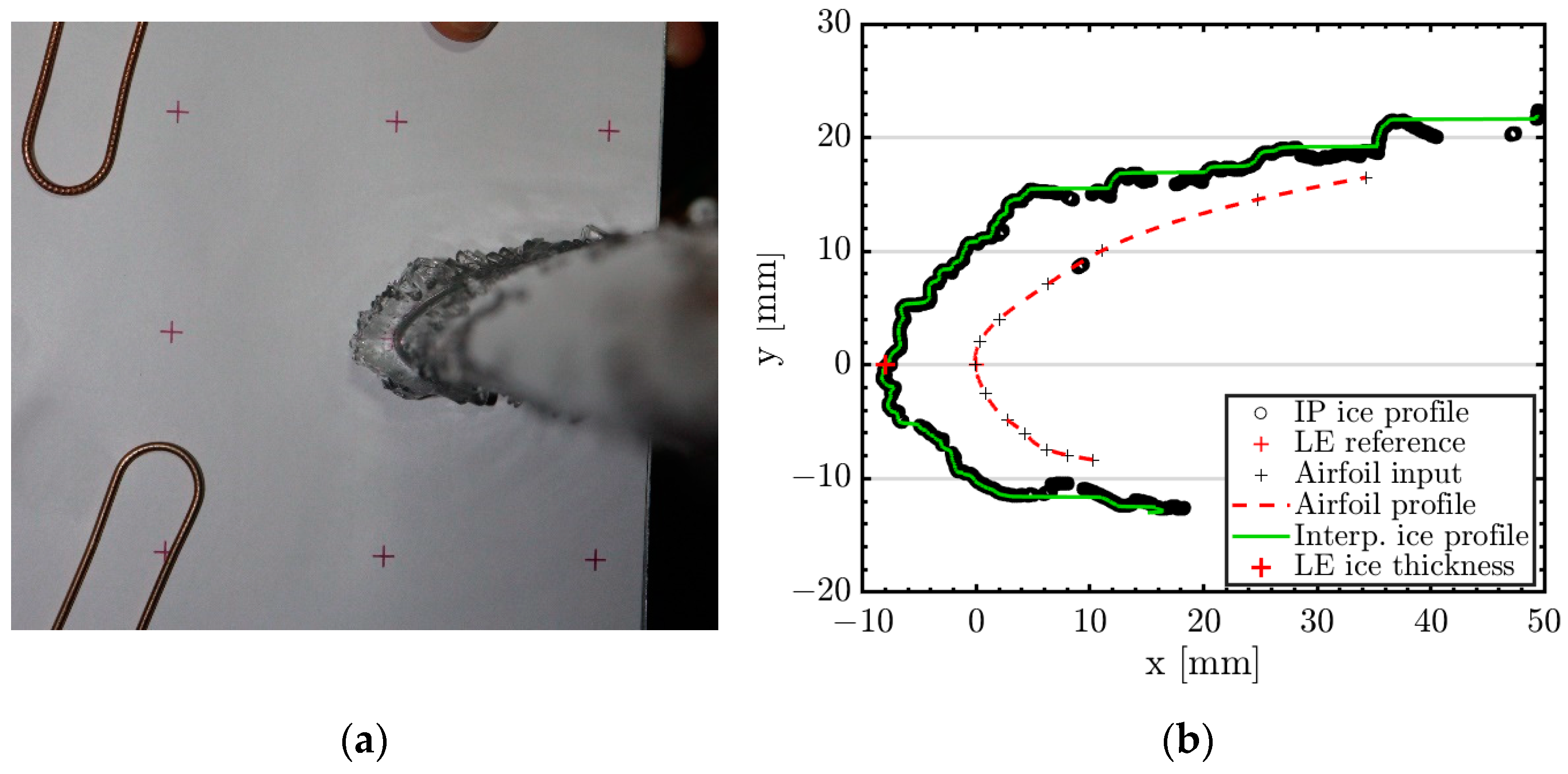
The first validation step of the developed measurement techniques was the validation of the leading-edge ice thickness—which was considered the reference parameter for the conducted ice accretion study. This parameter was chosen as, together with the accretion regime, it can be used to describe the icing event severity, to estimate its impact on the aerodynamic performance of the wings, to assess the optimal de-icing configuration of the ice protection system, and to predict the ice removal time. Moreover, the leading-edge ice thickness could be accurately measured during experiments using an electronic caliper. Therefore, these measurements could be used as exact values to evaluate the results obtained with the two post-processing methods: the image processing and the scan detection ice measurement techniques.
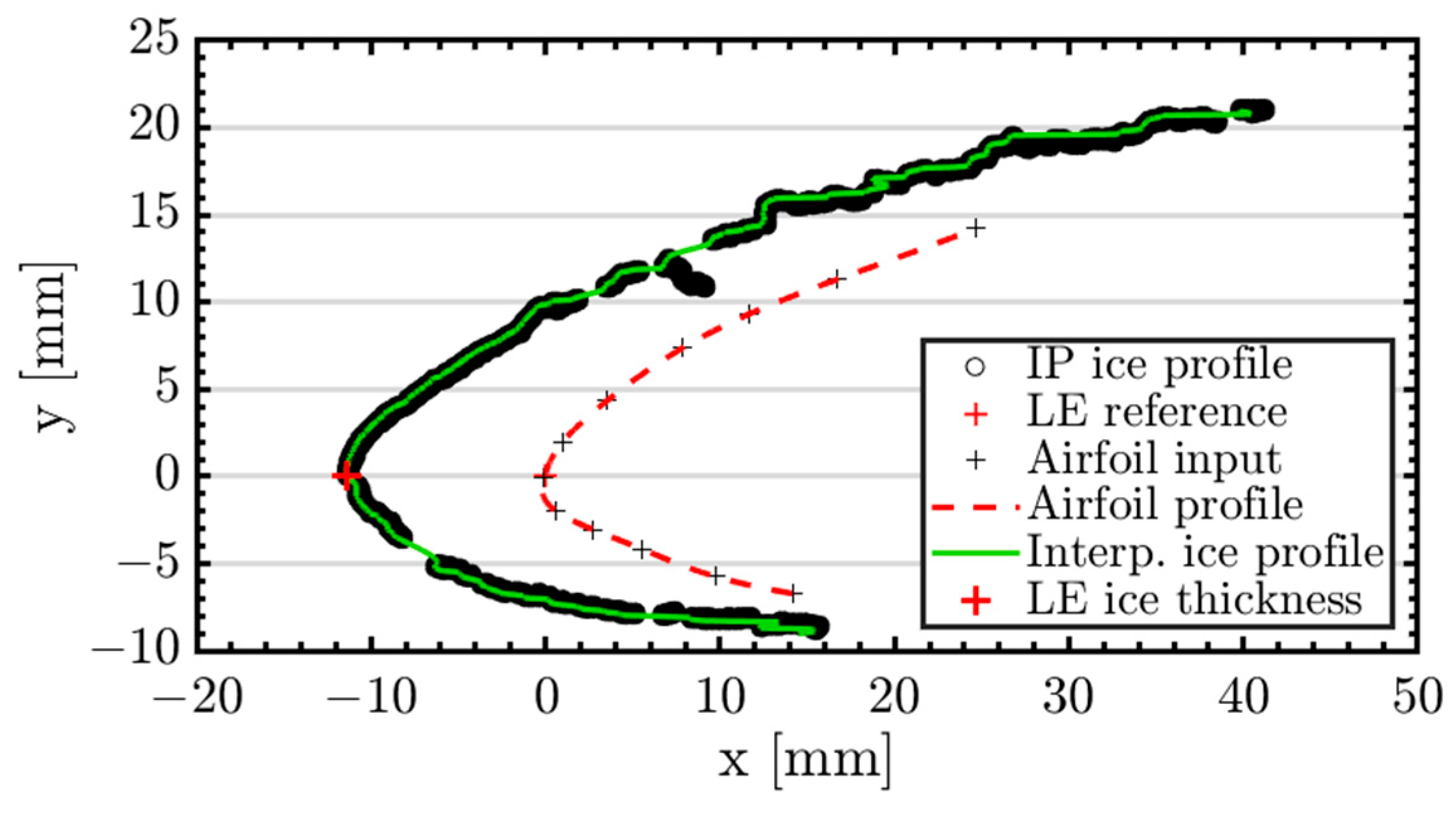
Both methods measure the leading-edge ice thickness by considering the same reference point (experimentally marked) on the airfoil’s leading edge, L (xLE, yLE) = L (0,0), and interpolating the detected 2D ice profile to determine the ice thickness value, xLE, at the yLE = 0 coordinate. Thus, the values obtained with both methods can be directly compared and validated against the caliper measurements. Also, a percentual error estimation—Equation (1)—is used to assess the performance of the post-processing methods.
E r r o r m e t h o d % = e c a l i p e r e m e t h o d e c a l i p e r · 100 ,  w h e r e   e  =  l e a d i n g  e d g e  i c e  t h i c k n e s s  [ m m ]
The numerical results employed in the validation of the image processing and scan detection methods against the experimental leading-edge ice thickness measurements are presented in Table 3. Both average absolute and percentual errors are presented for each technique. The first is obtained by averaging the absolute value of the difference between the caliper-measured thickness and the result of each method, and the second by averaging the absolute percentual errors for each method.
The leading-edge ice thickness caliper measurement trends are in line with the literature [9,
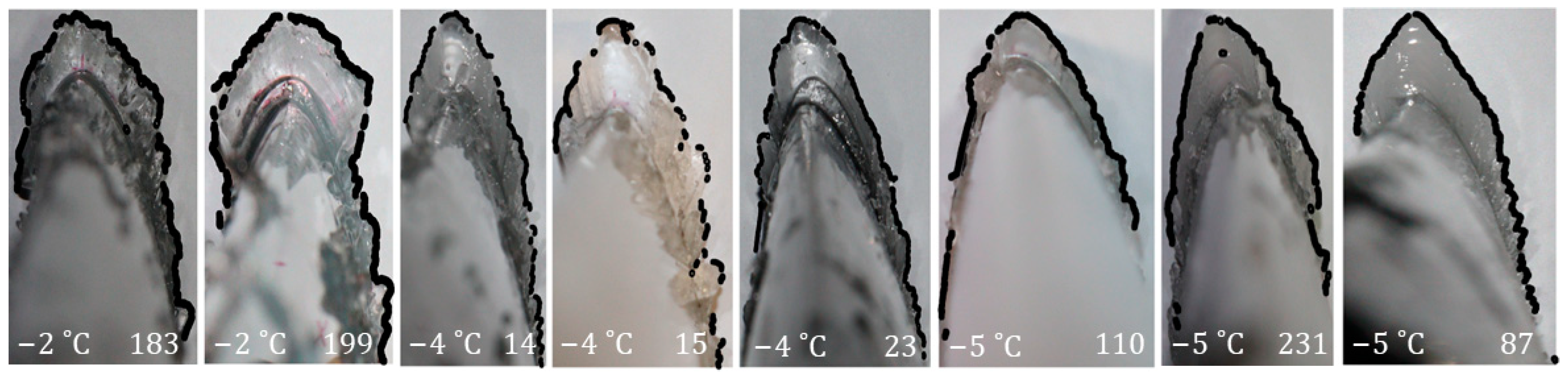
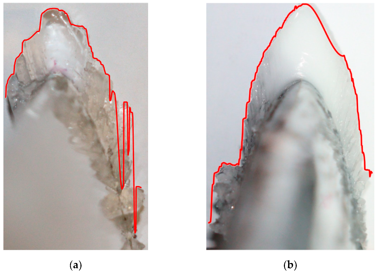
19]. The lowest ice thicknesses are observed for the highest IWT temperatures, T = −2 °C. The wetter airflow combined with the small temperature difference in the melting point generate a slow freezing regime in which the impinging water droplets do not freeze at impact with the airfoil, but instead travel downstream the profile and freeze later. This generates a transparent ice profile—glaze ice (Figure 13, cases 183, 199)—as the air entrapped in the freezing process is minimal, with a rounded shape and the lowest leading-edge ice thickness due to the movement of water droplets and low freezing rate.
As the testing temperature decreases, the melting temperature difference increases together with the freezing fraction. Hence, the water droplets freeze closer to the impingement point, which generates more streamlined ice accretion shapes with a pointy aspect in the leading-edge region. For the same ice accretion time and AOA = 0°, the leading-edge ice thickness increases with a decrease in temperature. During this faster freezing process, the air entrapment percentage increases, and more opaque ice shapes are observed with decreasing IWT temperatures—from almost transparent in the case of mixed ice at T = −4 °C (
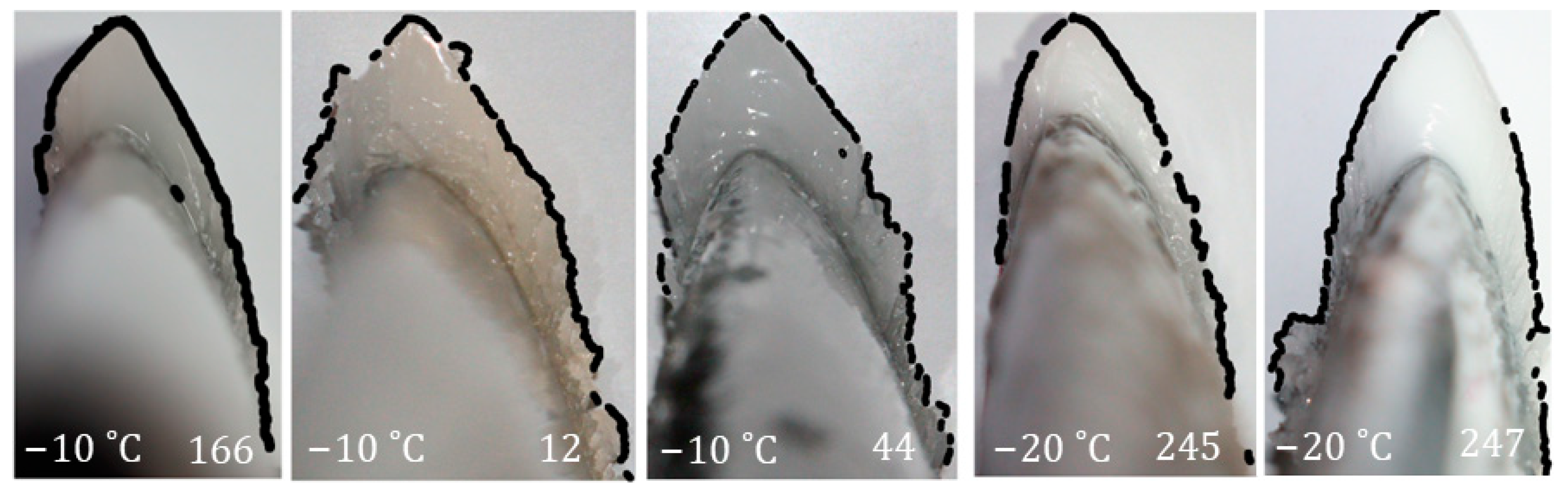
Figure 13, cases 14, 15, and 23) to milky white in the case of rime ice at T = −20 °C (Figure 14, cases 245 and 247).
Figure 13. Higher temperature range: T = −2, −4, and −5 °C, corresponding to glaze (183 and 199) and mixed (14, 15, 23, 110, 231, and 87) ice accretion regimes. The ice shapes are automatically detected in the experimental pictures by the image processing algorithm (detection drawn in black) and converted into 2D ice profiles (presented in Figure 15, Figure 16 and Figure 17).
Aerospace 10 00451 g013
Figure 14. Lower temperature range: T = −10 (runs 166, 12, 44) and −20 °C (runs 245, 247), corresponding to rime ice accretion. The ice shapes are automatically detected in the experimental pictures by the image processing algorithm (detection drawn in black) and converted into 2D ice profiles (presented in Figure 18 and Figure 19).
Aerospace 10 00451 g014
Concerning the numeric validation of the leading-edge ice thickness, both algorithms proved capable of capturing it. The results are in the same order of magnitude for all cases, regardless of the ice aspect, accretion time, or regime. By analyzing them based on the computed percentual error, the image processing method seems to capture more accurately the leading-edge ice thickness. Its maximal percentual error interval is from −4 to 6% of the error compared to the caliper data for all cases. For the scan detection method, the maximal error interval is one order of magnitude larger, from −23 to 24% over the entire testing range. As these are the maximal errors, it is beneficial to look at the absolute average percentual errors in order to better asses the techniques’ capabilities and to identify the cases in which algorithms perform best and the ones in which they lose accuracy. The average absolute percentual error in leading-edge ice thickness is ~2.2% for the image processing algorithm and ~9.5% for the scan detection method, and in terms of average absolute error values, these are ~0.26 mm for IP and ~0.98 mm for SD. This accuracy difference could be due to the increased number of steps in generating the scans for the second technique (manual drawing during IWT tests, post-test highlighting, and scanning) before the detection algorithm is applied, which could lead to an accumulation of errors. However, as both methods generate an absolute average percentual error lower than 10%, both techniques are considered validated for ice thickness measurements.
A more detailed error analysis allows for the identification of the drawbacks of each technique, an analysis which can be used for further improvement of the methods. The analysis of the first three highest error cases is presented below for each technique, while more general remarks and best practices with both methods are detailed in Section 4.
Concerning the IP method, the cases generating the highest percentual errors compared to the experimental leading-edge ice thickness value are cases 245, 14, and 15, with corresponding errors of 5.8%, −3.6%, and 3.4%, respectively. The first case is a rime ice accretion profile, while the last two are mixed.
For case 245, the 5.8% underestimation of the leading-edge ice thickness is believed to be generated by a slight misalignment of the calibration paper with the airfoils’ leading edge when the picture was acquired. As the ice shape is opaque, the prediction step of the IP algorithm was used to identify the LE cross position based on 3 reference points from the calibration paper. The resulting reference point is visibly higher than the airfoil’s leading edge but is in line with the other cross signs from the calibration paper. For case 14, the 3.6% overestimation is most probably due to a camera loss of ice shape perpendicularity. In the picture, the spanwise thickness of the ice cut can be observed at the top of the leading-edge ice. This small thickness is detected as part of the 2D ice profile and slightly increases the measured LE ice thickness value.
For case 15, the 3.4% underestimation is also possibly due to a small camera misalignment and a loss of perpendicularity, which is visible from the inclination of the leading-edge line towards the left of the image instead of going straight down. This might have generated a small perspective error which could have marginally reduced the measured leading-edge ice thickness.
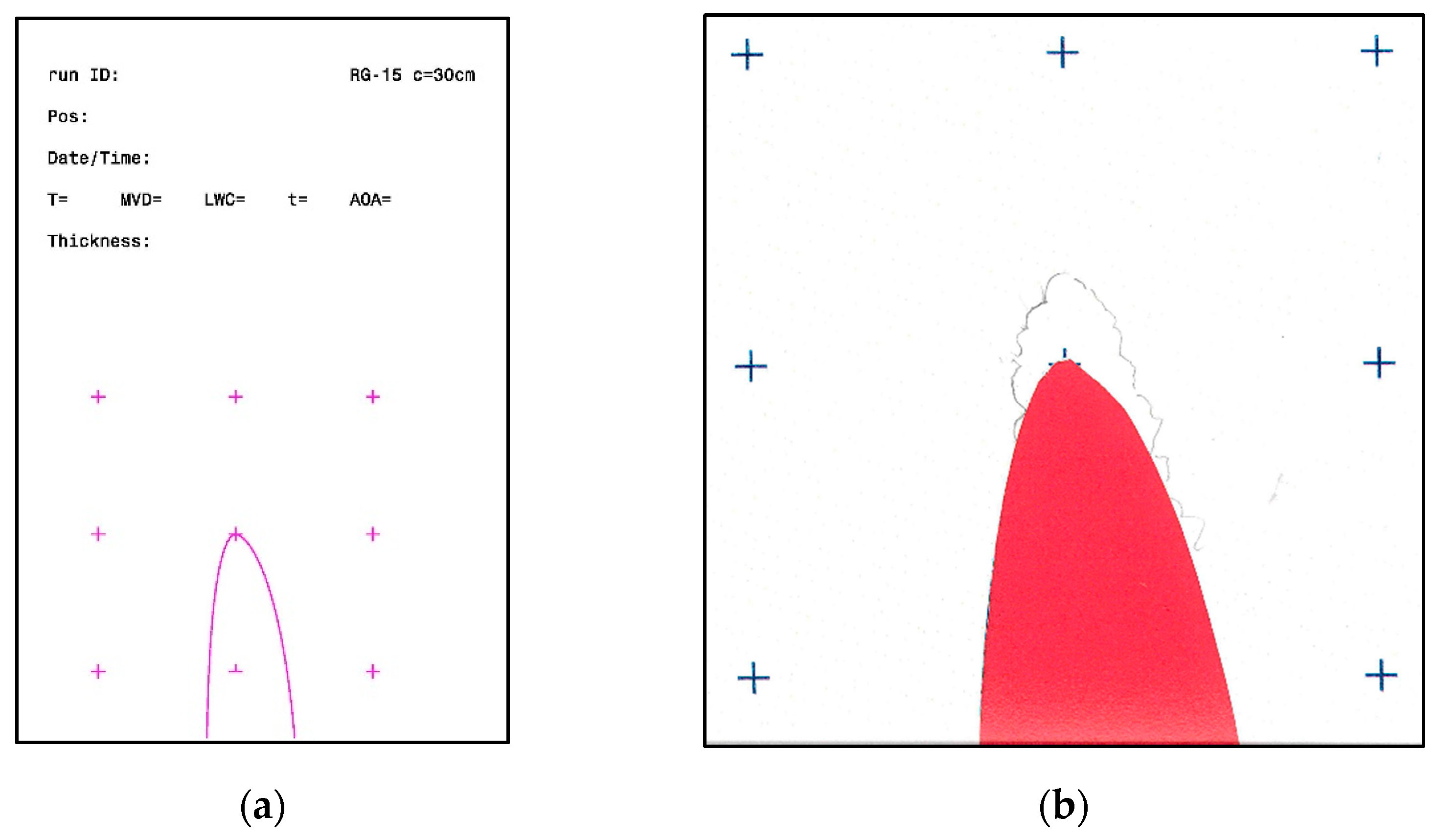
Regarding the SD method, the top three highest percentual errors are generated by cases 231, 110, and 12, with corresponding errors of 23.5%, −23.4%, and 18.3%, respectively. The first two tested cases are mixed ice accretion, while the latter is a rime accretion case.
Run 231 is the one with an angle of attack of 8°. Hence, the maximum thickness is not at the leading edge but is instead moved towards the pressure side of the airfoil. This makes it more difficult to measure the experimental leading-edge thickness with the caliper, which may cause larger uncertainties for the reference value. However, this increased uncertainty does not explain the 23.5% percentual error. An extended analysis of the possible sources of error for this case is presented in Section 3.3.
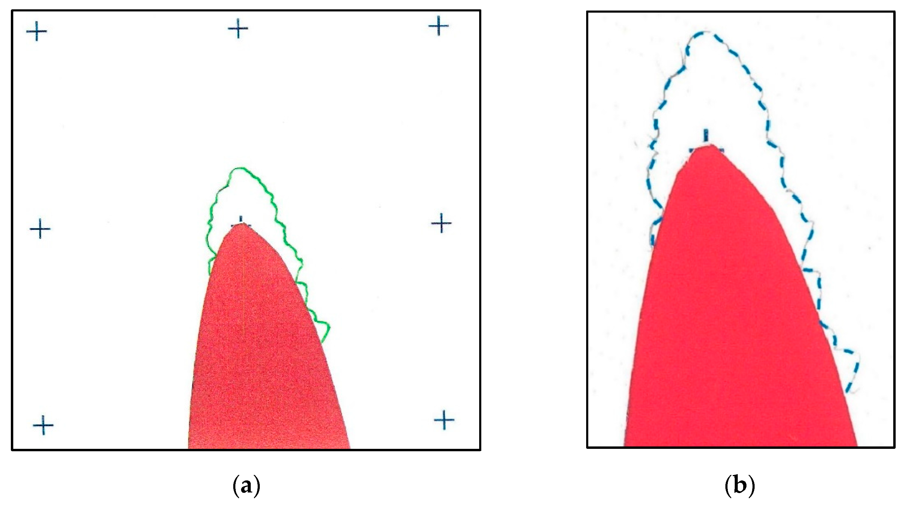
The overestimated ice thickness of the scan detection algorithm for run 110 is likely related to general uncertainties and the thickness of the green pencil. Typically, each scanned shape is printed on DIN A4 before re-tracing. In this case, the thickness of the green pencil could easily be 0.5 mm scaled into the original size. This can introduce a large relative error for small ice shapes such as the one in run 110. Additionally, the SD code tries to find the center of the line for stability reasons, although the innermost point would be a better representative of the actual ice shape.
The maximum thickness for the traced ice shape from run 12 is not at the leading edge but is instead moved slightly towards the suction side. When taking the maximum thickness of the SD profile in close vicinity of the leading edge, the thickness matches the caliper measurement much better. This could indicate that the paper template was not in the correct position and was slightly rotated. A second explanation would be that the maximum thickness might have been rotated from the leading edge, and, similar to run 231, the caliper measurement has a higher uncertainty. Additionally, the original tracing has many lines close to the leading edge. Hence, re-tracing is a more difficult process for this ice shape and could lead to higher errors.

3.2. 2D Profiles Comparison

In order to facilitate comparison of the 2D ice profiles obtained with both codes, the profiles’ positions were corrected by rotating one of them to align the airfoils’ leading edge, aiming for a perfect alignment, especially on the wings’ suction side. The comparison results are presented in Figure 15 for the glaze ice accretion regime, in Figure 16 and Figure 17 for the mixed one, and in Figure 18 and Figure 19 for rime ice.
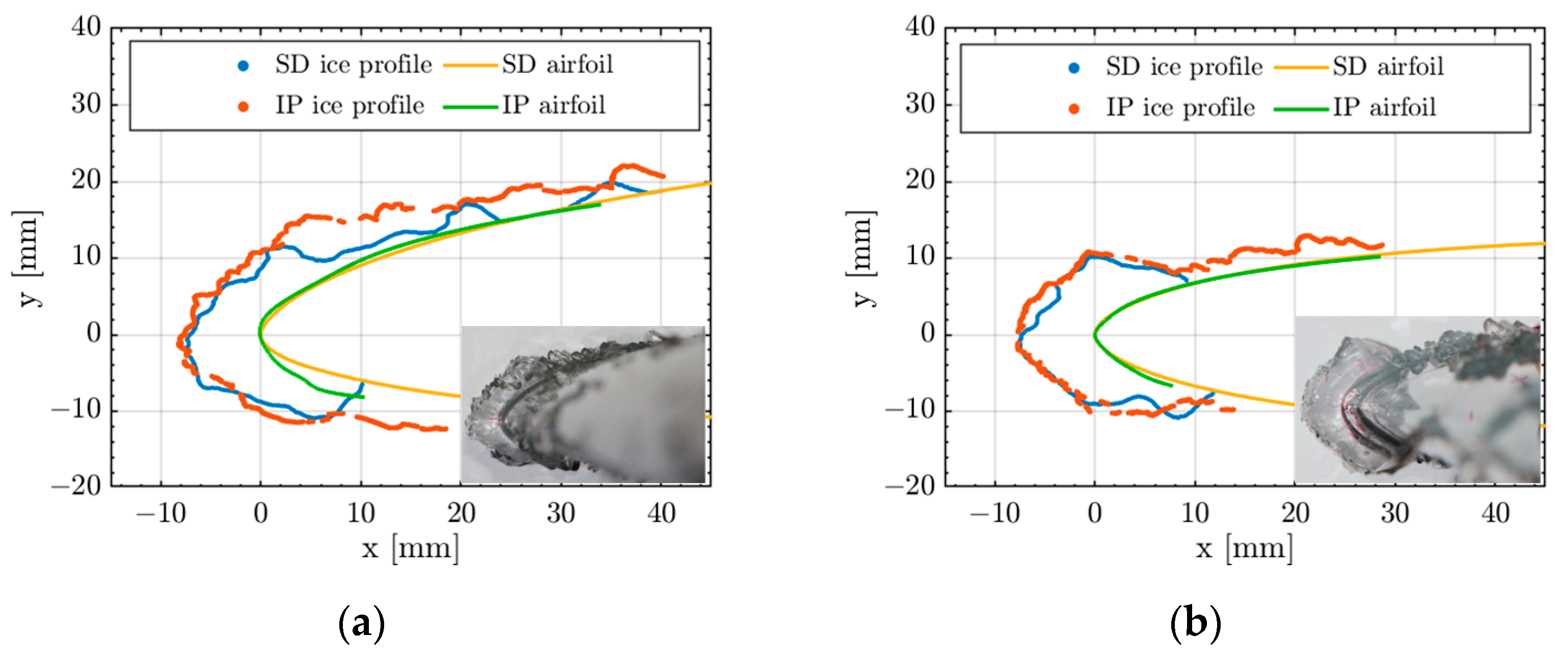
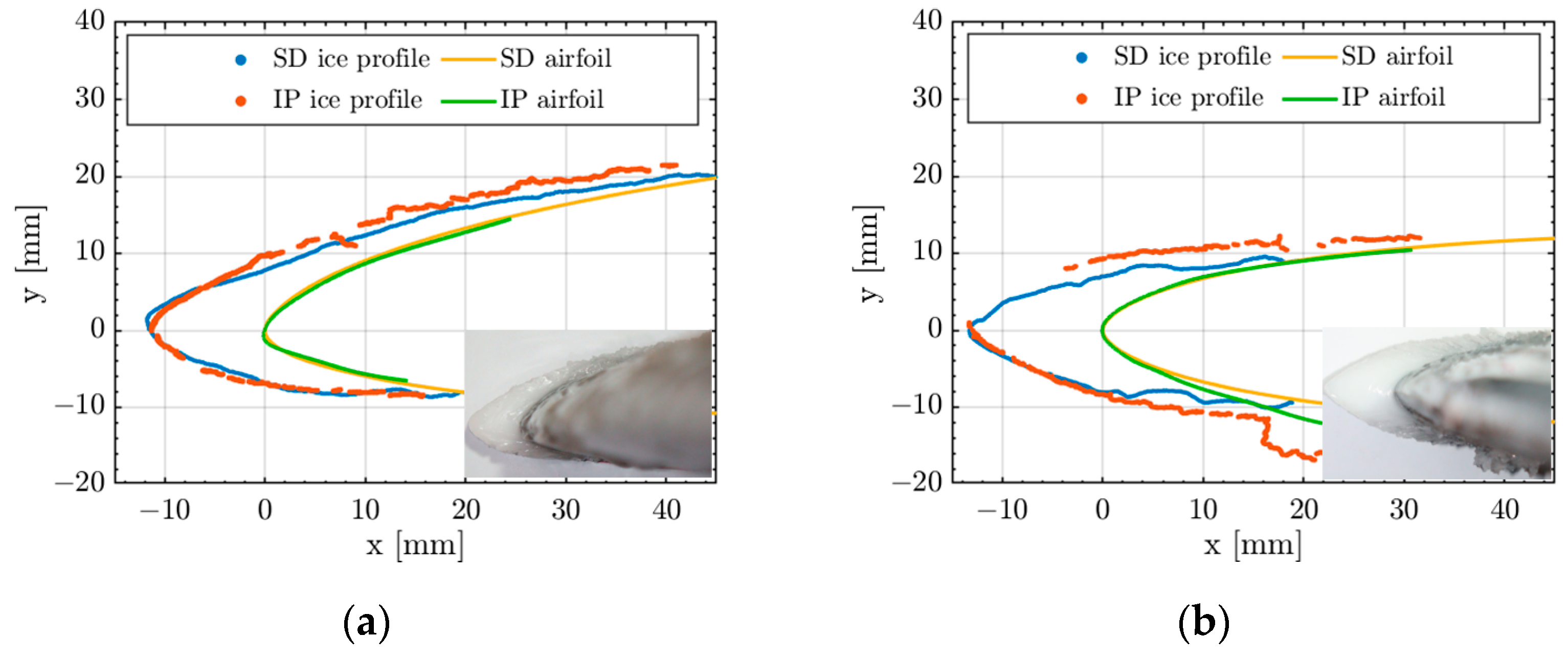
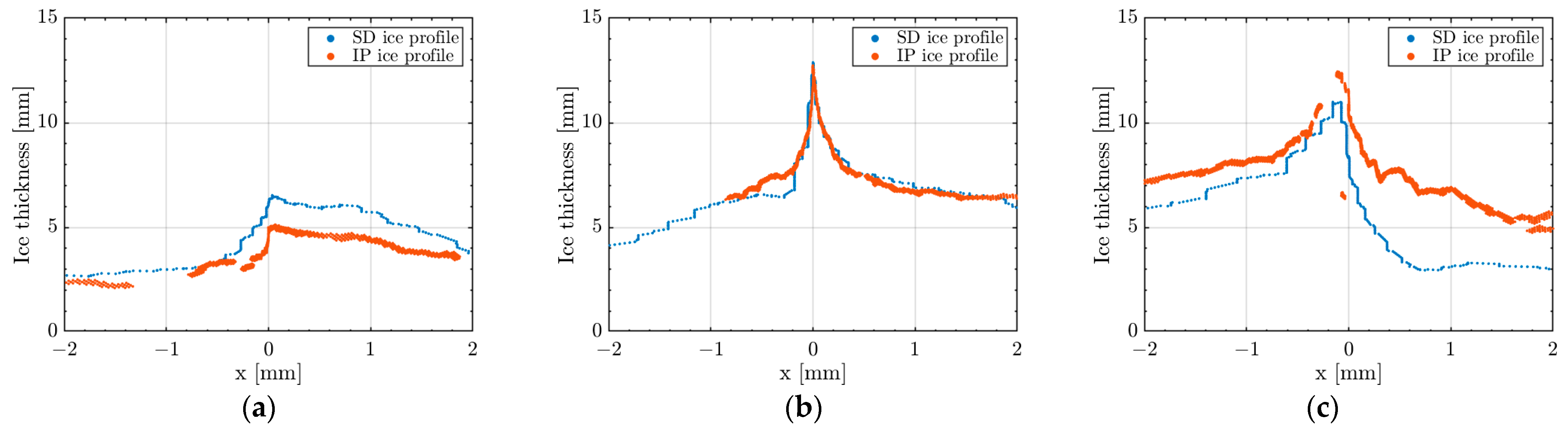
Figure 15. 2D glaze ice accretion profiles (T = −2 °C)—comparison between the image processing (IP) and the scan detection (SD) techniques—for (a) run 183 and (b) run 199.
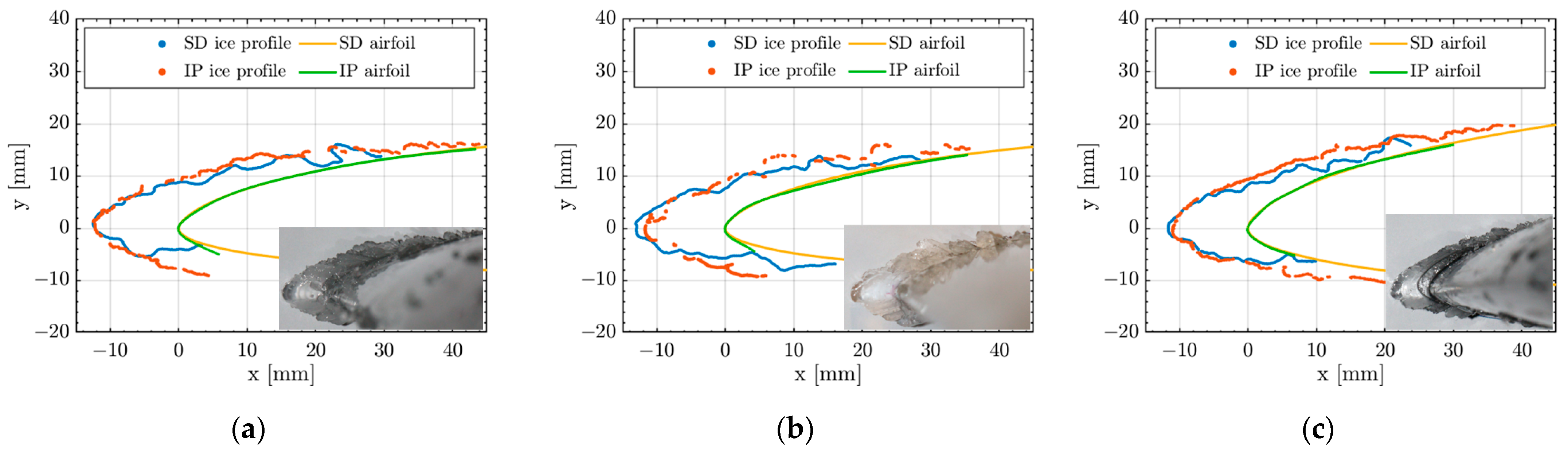
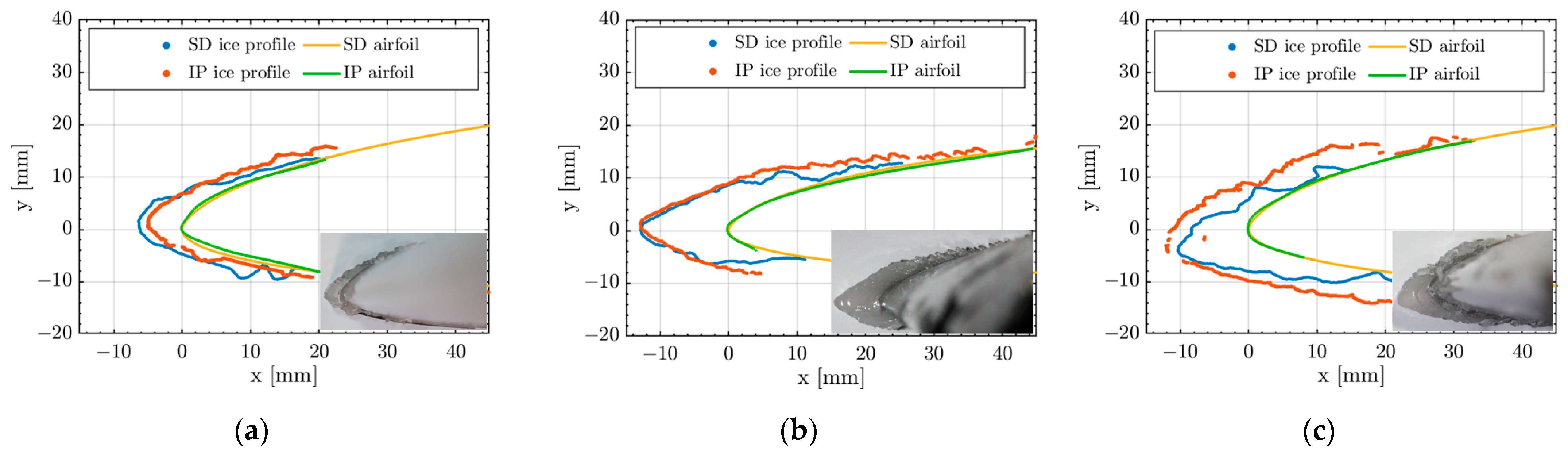
Aerospace 10 00451 g015
Figure 16. 2D mixed ice accretion profiles (T = −4 °C)—comparison between the image processing (IP) and the scan detection (SD) techniques—for (a) run 14, (b) run 15, and (c) run 23.
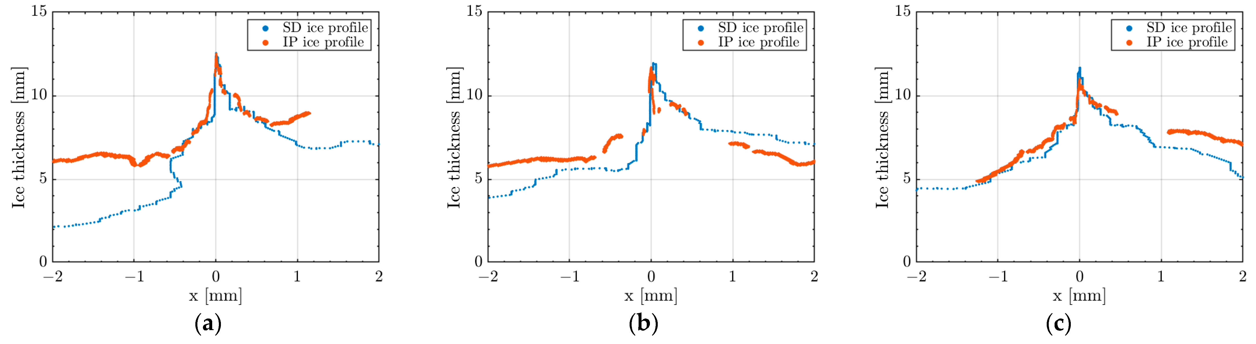
Aerospace 10 00451 g016
Figure 17. 2D mixed ice accretion profiles (T = −5 °C)—comparison between the image processing (IP) and the scan detection (SD) techniques—for (a) run 110, (b) run 87, and (c) run 231.
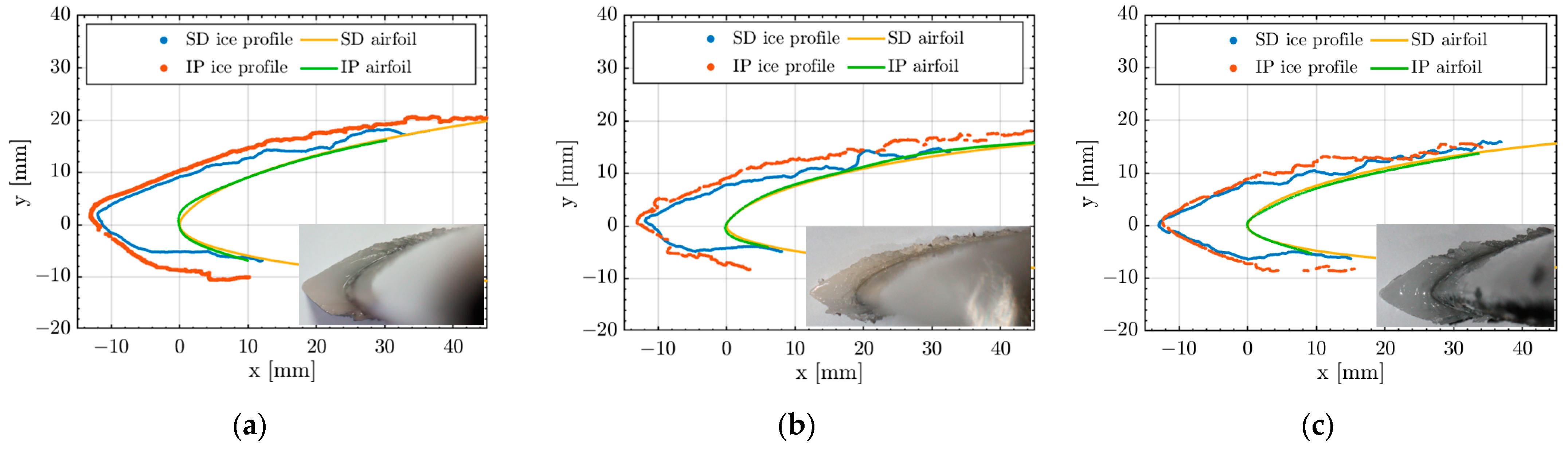
Aerospace 10 00451 g017
Figure 18. 2D rime ice accretion profiles (T = −10 °C)—comparison between the image processing (IP) and the scan detection (SD) techniques—for (a) run 166, (b) run 12, and (c) run 44.
Aerospace 10 00451 g018
Figure 19. 2D rime ice accretion profiles (T = −20 °C)—comparison between the image processing (IP) and the scan detection (SD) techniques—for (a) run 245 and (b) run 247.
Aerospace 10 00451 g019
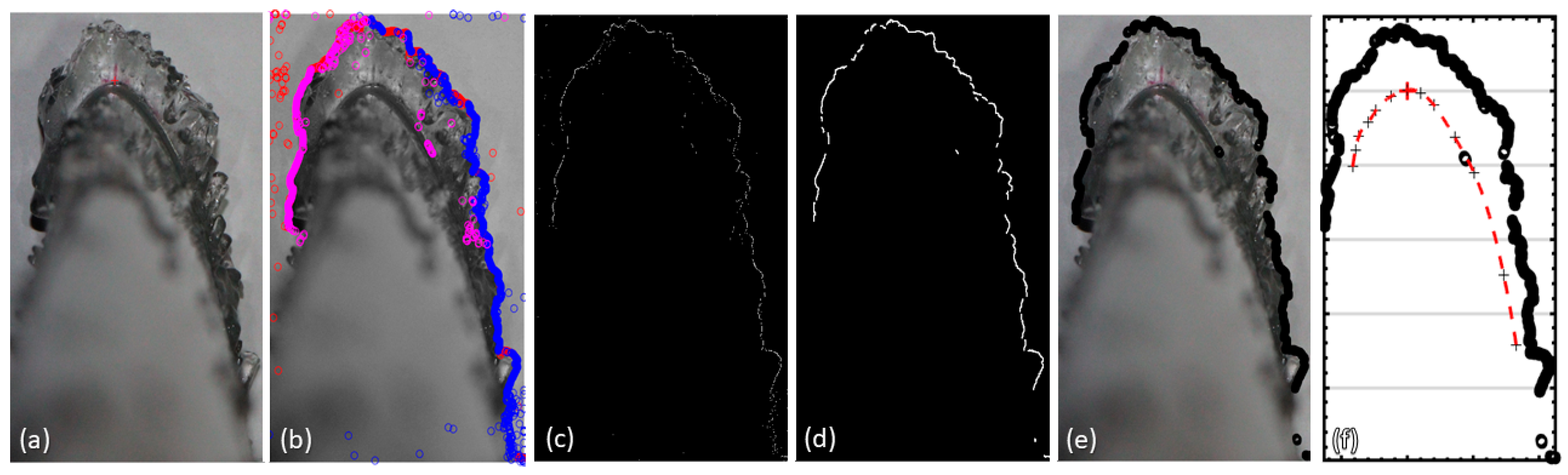
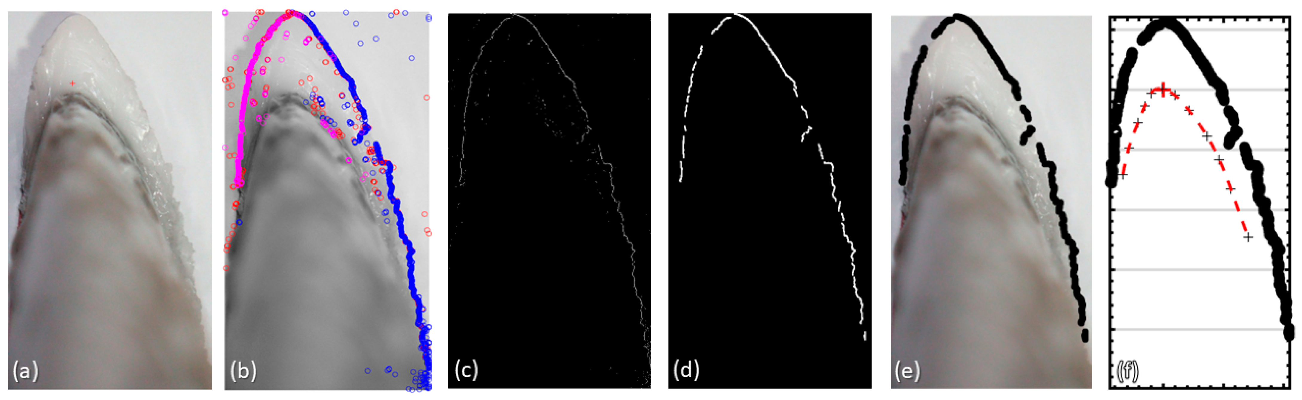
The airfoil alignment between both techniques is achieved in all cases—finding a good agreement between the pre-cut metal airfoil shape used for the SD technique and the IP obtained profile. This proves that the image pre-processing corrections were well applied, as the IP algorithm generates a virtually undistorted airfoil profile.
Based on this observation, the obtained 2D ice shapes are also considered to be unaffected by distortion. In some cases (as in Figure 15a,b and Figure 16a,b and Figure 19b), the IP-generated airfoil profile diverges from that of the SD downstream of the leading edge on the pressure side. This occurs because, in pictures, the pressure side appears blurred due to a difference in perspective, as the camera is aligned and focused on the suction side and leading-edge sides. For this reason, the airfoil profile is not clearly defined in the pressure side area, and errors can occur in the manual selection of the airfoil points. Greater airfoil profile abnormalities could occur if the wing span is not completely ice-free and ice is remaining along the optical path which is integrated in the blurred region, thereby generating an airfoil profile distortion (as with run 183 in Figure 13 and Figure 15a). However, these airfoil profile abnormalities do not affect the quality of the ice profile detected by the IP method, the two profiles being generated in different manners, as is detailed in Section 2.
The qualitative comparison of the 2D ice shape results shows that the image processing and the scan detection techniques generate comparable profiles, which, in most cases, overlap and capture the same features of the ice profile. The absolute ice thickness values have some discrepancies, especially in downstream regions.
However, a significant difference between the results of the two methods is observed in terms of line continuity: the SD method generates a continuous line, while the IP ice shape profiles are sometimes interrupted, and they do not always connect to the airfoil at the ends. This occurs because the pre-processed SD profiles are hand-drawn, starting and ending at the airfoil’s surface, while the airfoil–ice interface is not always clearly visible in the images employed by the IP method. This is because the camera integrates the airfoil’s surface in the spanwise direction, and a blur effect occurs in the regions to which the camera is not perfectly perpendicular (visible in, e.g., Figure 14, run 166). The interrupted aspect of the IP profiles is due to the filtering step applied in the post-processing to correct for detections of shadow (e.g., Figure 14, run 247) or light reflections (e.g., Figure 13, run 15) which could influence the measurement if not excluded. Afterward, an analysis based on the testing temperature ranges was performed in order to assess the applicability of these methods to certain ice accretion regimes. The best agreement was observed for the rime ice shapes, which correspond to the lowest IWT temperature regimes (T = −10, −20 °C) and are depicted in Figure 18 and Figure 19. The streamlined ice shape is specific to rime accretion, with the highest ice thickness being present in the leading edge and decreasing downstream of the airfoil, and a relatively smooth surface is well captured by both methods. The profiles overlap in the leading-edge region and maintain a similar shape and thickness size, although the IP ice profiles continue a bit further downstream on the airfoil and present more roughness (in the form of small irregularities) than the SD ones. This could be explained by the fact that the SD profiles are limited by the size of the drawing paper and the metallic support, while the IP processes the field of view captured by the camera in the image. Also, the small roughness variation is mostly dampened in the hand-drawing process of the profile, which precedes the SD processing. Therefore, the SD profiles appear smoother. The IP profile may appear slightly ampler than that of the SD towards the airfoil’s tail, and the ice thickness in this region may be marginally increased in some cases. This is because, for non-transparent ice shapes (rime or mixed), the thickness of the 2D ice cut might be visible in the image towards the downstream airfoil area. The camera’s sensor starts to be misaligned and lose perpendicularity to the ice shape in the downstream area as it is focused on the airfoil’s leading edge. This does not always occur, and its effect is considered to be negligible, as discussed in Section 2.2.
For the temperatures corresponding to mixed ice accretion (T = −4, −5 °C), the profiles captured by the two techniques show a good agreement on the general shape, generally matching both the leading-edge ice thickness and the downstream ice evolution. Both techniques present more ice shape irregularities and capture the increased roughness of this accretion regime (e.g., visible ice feathers in Figure 13, run 14,15). However, these formations do not perfectly overlap between the two profiles. This suggests a possible camera misalignment error with loss of perpendicularity to the ice profile (most noticeable in Figure 13, run 15, by observing the inclination of the airfoil’s leading-edge line towards the left side of the image instead of straight down as in run 23, where the camera is well aligned). This misalignment is visible in the results’ comparison (Figure 16, run 15), which shows an ~1 mm vertical offset between the SD and the IP profiles. This vertical offset generates further misalignment of the ice irregularities in the downstream region of the two ice profiles. Methods to avoid these errors are recommended in Section 4. Based on the leading-edge thickness validation and the agreement between the 2D ice shapes generated with the SD and IP methods, the errors introduced by this misalignment are considered negligible, and the ice profile is representative of the studied mixed ice accretion cases.
For the highest testing temperatures, (T = −2 °C), the glaze ice profiles are well captured by the two 2D measurement techniques. The results from both the SD and IP algorithms measure the leading-edge ice thickness with errors below 7.5% and 2%, respectively, compared to the experimental value. In addition, both methods capture the leading-edge horns well, together with the downstream ice protuberances (Figure 13, run 183 and 199). Although both methods capture all the details of the profiles, there is less overlap than for the rime and mixed ice accretion regimes (Figure 15a,b). This discrepancy could be due to the ice’s characteristics, which, in this case, forms in a wetter regime, has a more complex shape, and has a transparent appearance. The first two differences possibly increase the uncertainty during the manual drawing step of the SD technique, as the increased ice slippage and required level of detail make the drawing prone to more errors. Moreover, the drawing is made against the support paper, thereby acquiring a purely 2D profile for the SD method. For the IP method, the picture is prone to encompassing some 3D effects in this case, as the ice has an increased complexity, with its aspect varying along the span of the cut. Thus, combined with the ice’s transparency, the resulting 2D profile is more the ice shape integrated along the ice cuts’ thickness. To achieve high accuracy, the ice cut should be kept as thin as possible, but in this case, it is ~1 cm. Therefore, the slight discrepancy between the 2D profiles generated with the two methods is not concerning, especially as the general aspect is conserved. By keeping in mind how each technique acquires and processes the profiles, both can be used to generate representative 2D ice shapes for glaze ice accretion.

3.3. 1D Ice Thickness Results

The 1D thickness ice profile represents an algorithm that was developed to geometrically linearize the 2D ice shapes and to facilitate the direct comparison of the ice accretion results regardless of the airfoil shape. The algorithm can be applied to digital 2D ice profiles generated by any technique (SD, IP, or other), as long as an ice profile is provided with the corresponding airfoil points. Subsequently, it generates a graph with the ice thickness for each airfoil surface point.
The 1D thickness algorithm allows for fast identification of the ice accretion regime from profiles’ characteristics, such as leading-edge ice thickness, maximum ice thickness, ice coverage, profile aspect, etc., a fast investigation of the icing severity, and easier approximation of the accumulated ice mass for a given profile.
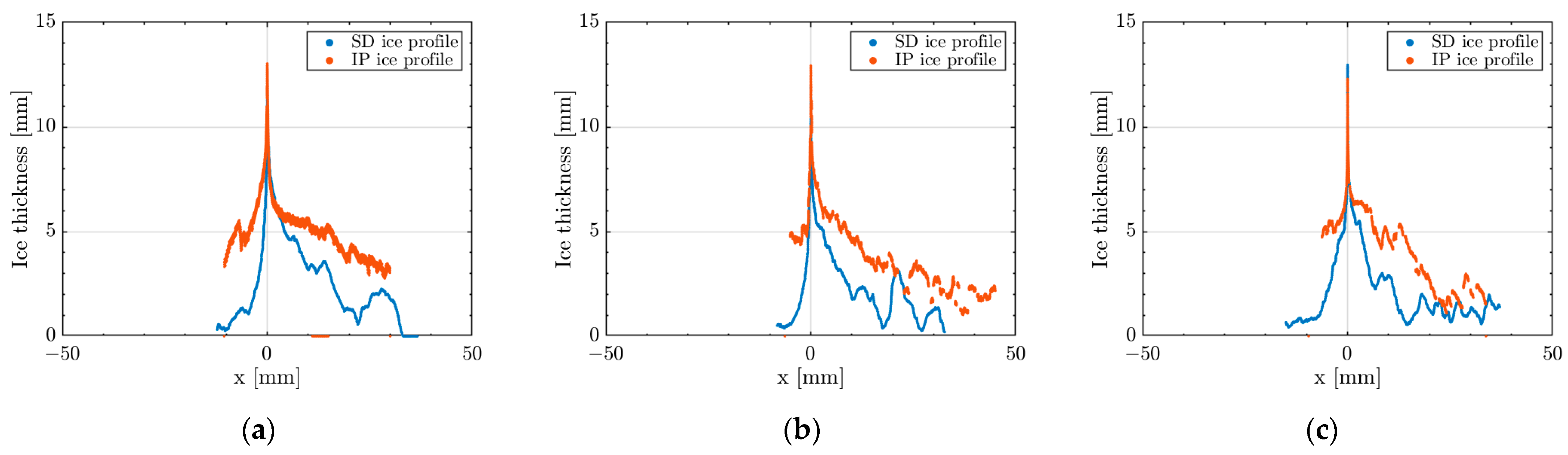
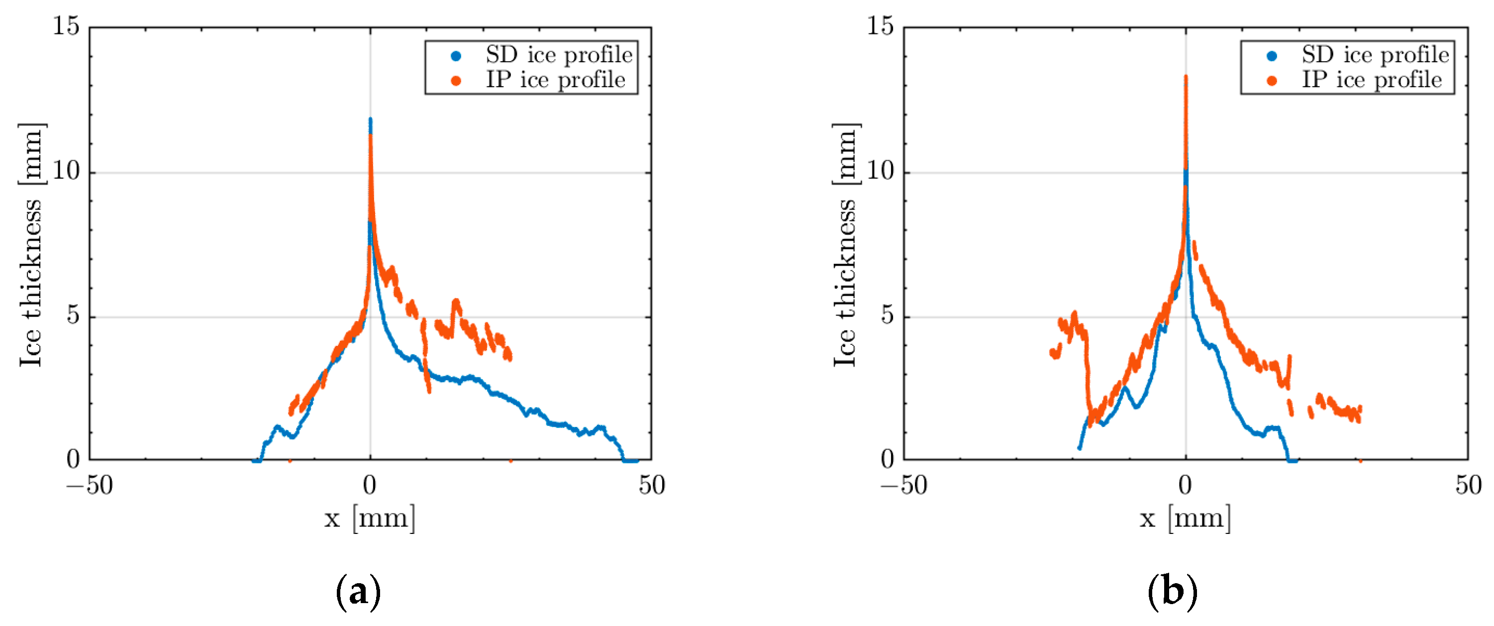
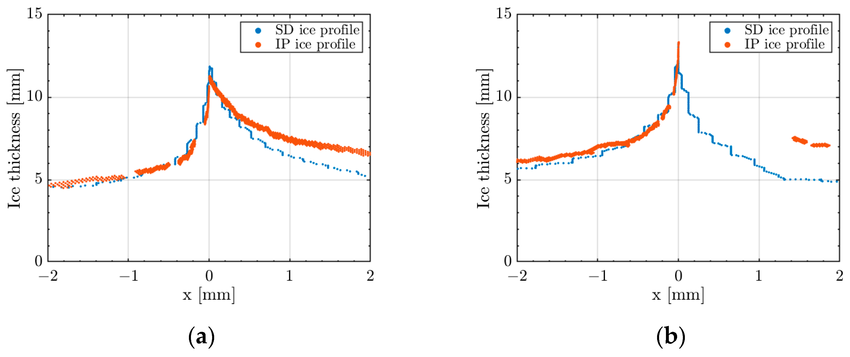
The rime ice accretion regime can be easily identified from the 1D profiles. The profiles present a very important ice thickness in the stagnation point (in this case, on the [0,0] point of the leading edge, as the airfoils were positioned at a 0°AOA)—Figure 20 and Figure 21. A detailed view of the stagnation point region can be found in the Appendix C, Figure A4. The rime ice accretion profiles present the highest leading-edge ice thickness between all studied cases as the impinging water droplets freeze at impact with the airfoil. From this point downstream, there is a steep decrease in ice thickness on both the negative and the positive sides (pressure side and suction side, respectively), followed by a relatively smooth and gradually decreasing ice profile, which represents the streamlined rime ice accretion aspect. For most cases, the ice spreads further downstream on the airfoils’ suction side (x positive), which is expected, due to the increased air speed along this part due to the cambered airfoil shape (RG-15). For run 247 (Figure 21b), the ice is approximately evenly spread, as the tested airfoil (SD8020) has a symmetric shape.
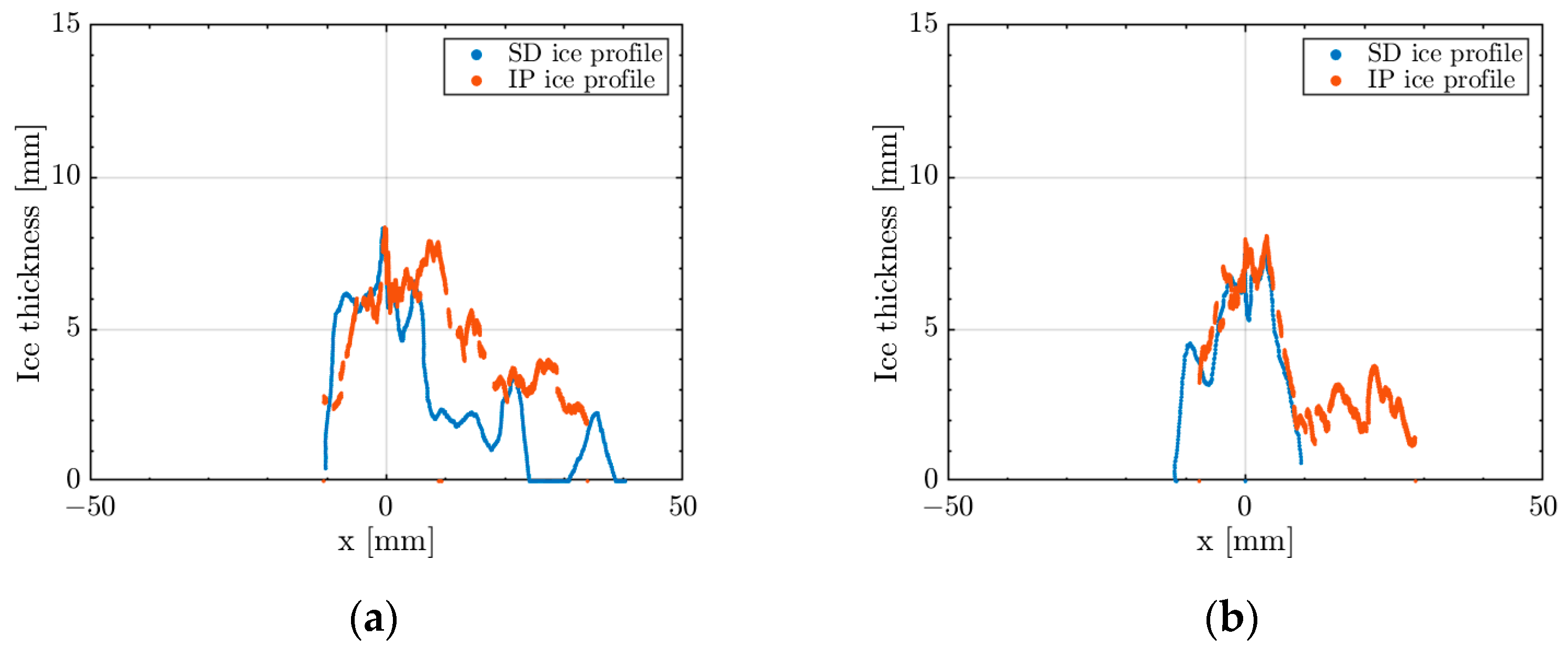
The glaze ice 1D profile can be identified as having the opposite characteristics of the rime ice profile. There is a significant amount of ice in the stagnation point, but its thickness is comparable with the thickness of the ice horns—other ice protuberances formed close to the leading edge, which can be noted as spikes in Figure 22a,b. These occur as, due to the high temperatures close to the melting point, the water droplets do not freeze upon impact, but instead travel downstream of the airfoil profile and freeze at different locations. This generates a more even 1D ice profile, where the central region has the highest ice thickness values, followed by significantly shorter ice protuberances downstream (in these cases, on the x-positive suction side).
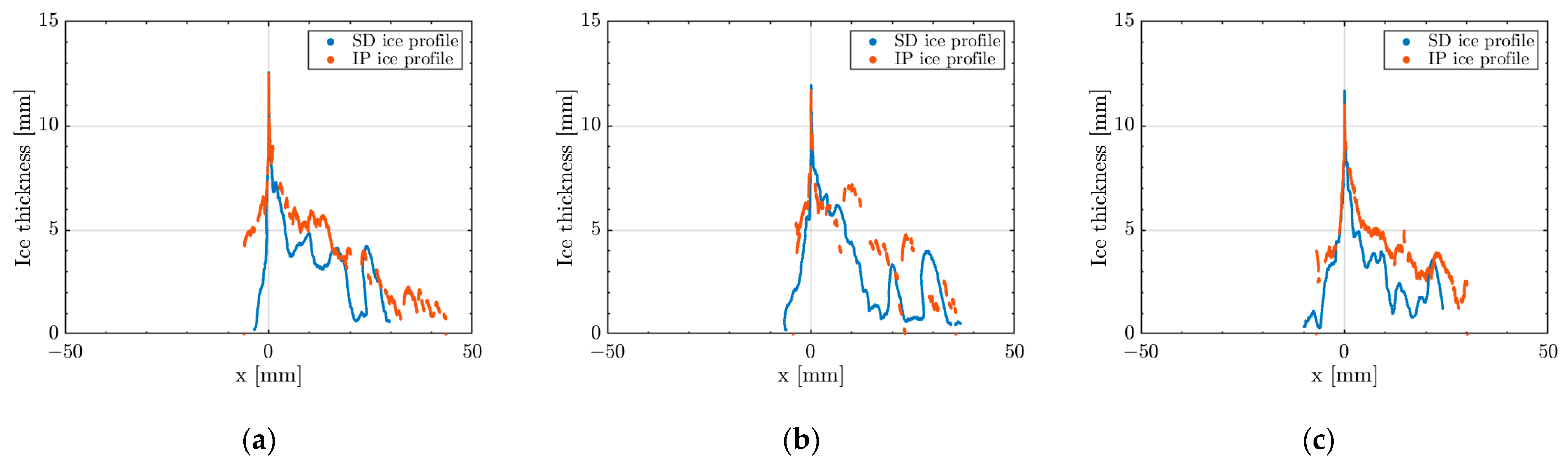
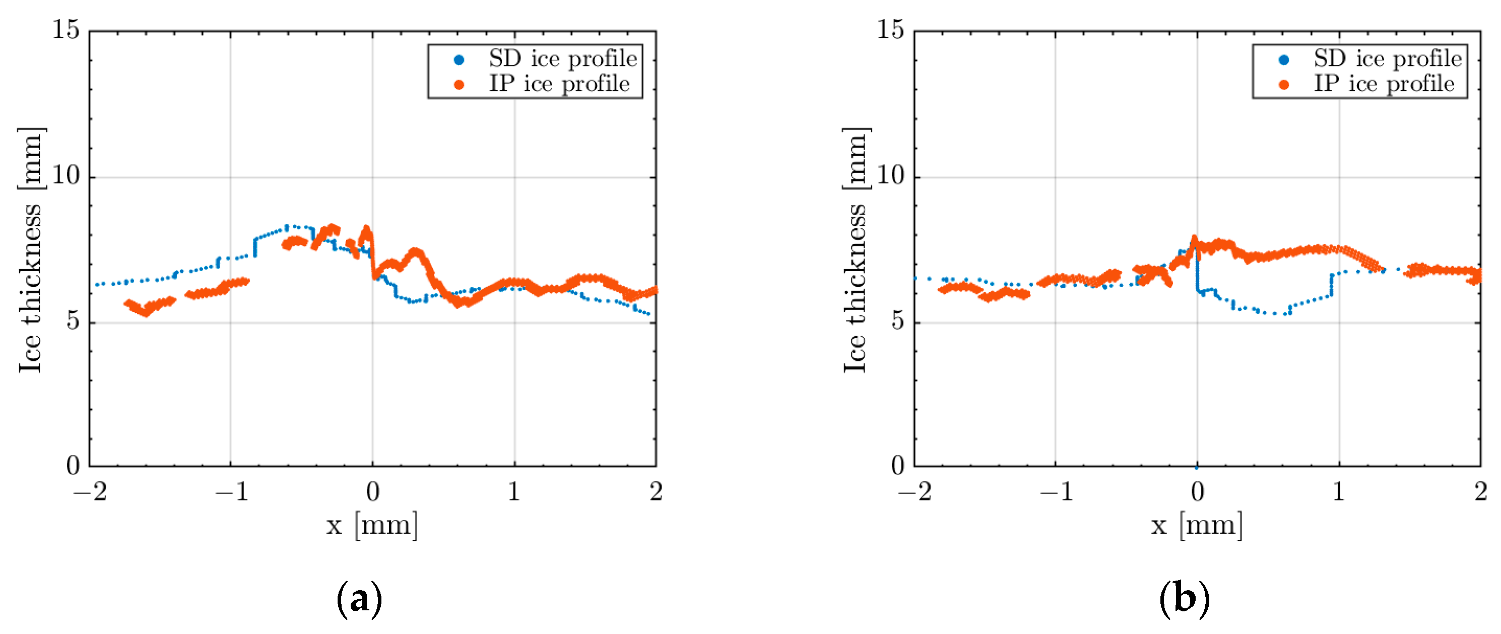
The mixed ice regime generates 1D ice profiles with combined characteristics from the two previous ice accretion regimes. As with the rime ice profiles, it is characterized by the highest ice thickness present at the stagnation point (Figure 23 and Figure 24), followed by a less steep decrease in ice thickness downstream on the profile, with a high roughness region (Figure 24) and ice spikes which represent the 2D ice protuberances and ice feathers (Figure 23). Two atypical results are observed in Figure 24a,c. These correspond to experiments performed to test slightly different conditions, such as the impact of the ice accretion time or of the airfoil’s AOA over the ice shape profile. At the same time, these runs also test the measurement techniques’ capabilities.
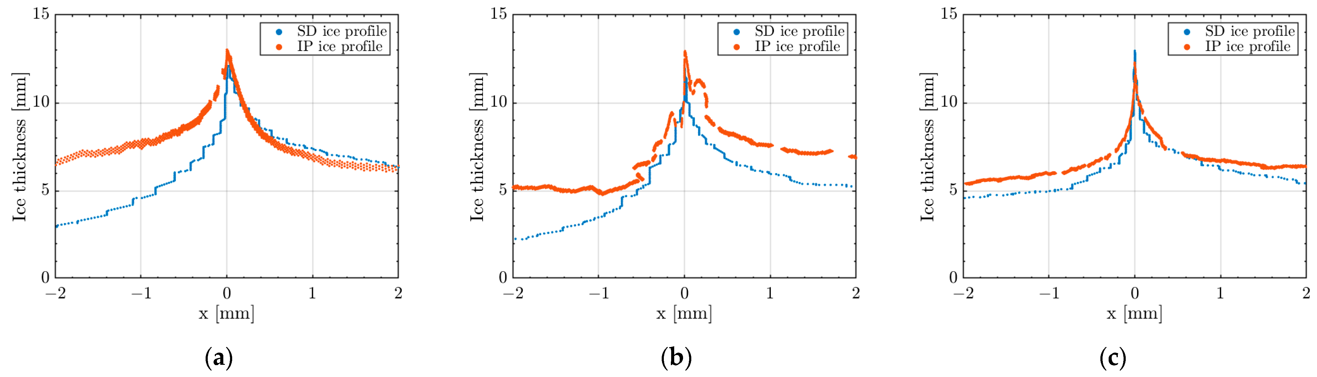
First, run 110 was tested in order to investigate the ice accretion severity and shapes for a reduced ice accretion time (8 min instead of 20). The amount of accreted ice is reduced because of the reduced ice accretion time. The thickness is still quite evenly distributed around the leading edge, with some visible roughness formations downstream and with an already-formed ice peak at the stagnation point. Despite the reduced accretion time, the ice accretion regime can still be easily identified from the ice thickness profile.
Second, run 231 was tested at the general ice accretion time, but with the airfoil positioned at an increased AOA (8° instead of 0°). This experimental configuration was tested in order to observe its impact on the ice shape profile, especially on the position of the maximum ice thickness. A detailed view of the Figure 24c profile is presented in the Appendix C, (Figure A7), where the maximum ice thickness position can be easily identified at about –0.1 mm, thus 0.1 mm below the leading edge’s highlight point on the airfoils’ pressure side.
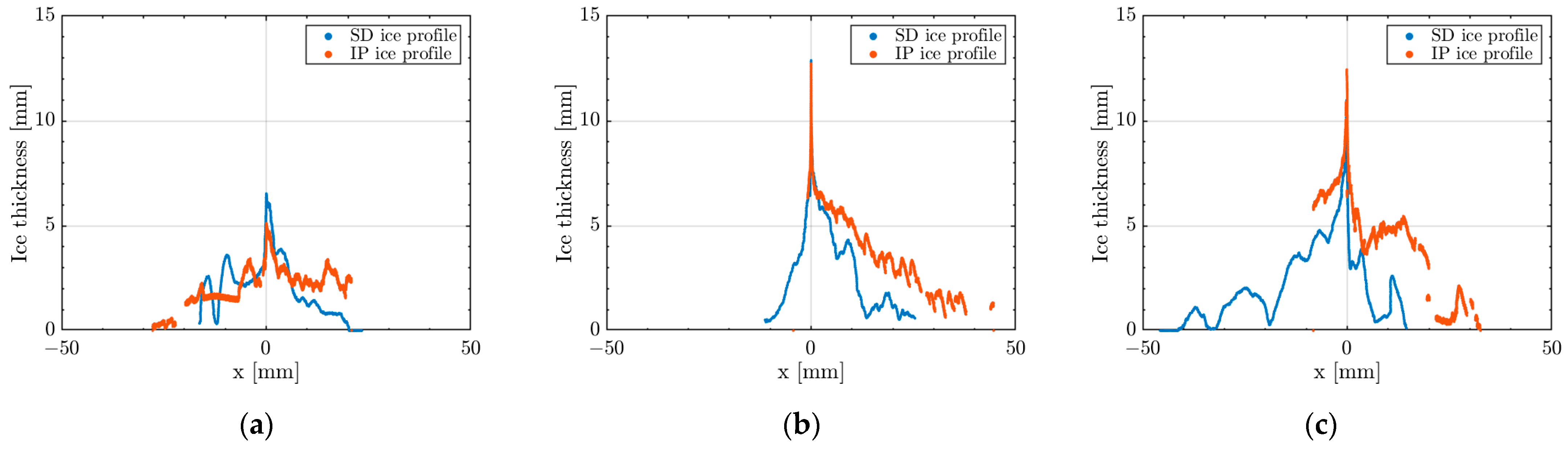
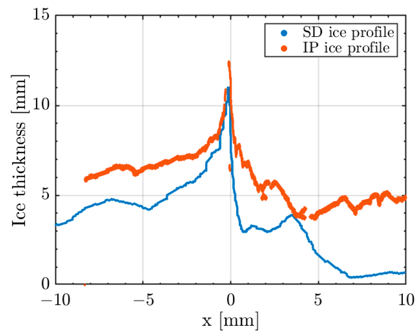
Moreover, for this particular run (231), the 1D thickness analysis was useful in identifying the other sources of error which motivate the 23.5% leading-edge ice thickness error for the SD method (Table 3) and for the differences in 2D profiles between the two techniques (Figure 17c). From a detailed view of the 1D thickness profiles’ comparison (Figure A7c), it was observed that the profiles were highly similar in the leading-edge region while having an offset of ~1.2 mm. An enlarged detail of the leading-edge region reinforced the profile similarity (Figure 25). A closer investigation of the raw data for the 2D ice shape measurement techniques (presented in detail in the Appendix D, Figure A8) suggests the misalignment of the support paper before the profile hand-drawing of this run. This seems to have misplaced the LE marker further in the positive x direction of the 2D profile, thereby losing the leading-edge contact point with the airfoil. This might have generated the ~2 mm-lower LE ice thickness value of the SD method. The misalignment was not noticed during the experiments. It is considered to be the most important source of error for the SD method in this case, with the influence of the increased caliper measurement uncertainty having only a secondary effect. Regarding the IP result for this run, the misplacement of the alignment paper did not represent an issue, as the optical path was clear and the airfoil’s leading edge was identifiable directly from the image. Moreover, its error of 1.3% is within the uncertainty interval of the IP measurement method.

4. Discussion

In this section, a comparison of the two techniques’ capabilities is presented. For each method, the accuracy, the applicability, the advantages and disadvantages, and the possible sources of error are analyzed. Advice for maximizing the methods’ efficiency and accuracy is summarized in a best practice guide, and possible improvements are suggested. The methods’ capabilities are again compared to the measurement techniques available in the literature, mostly in terms of cost and availability.
As observed in Section 3, both the scan detection and image processing 2D ice shape measurement methods can generate meaningful results for all of the tested ice accretion regimes (rime, glaze, and mixed) in terms of leading-edge ice thickness and 2D ice profiles.
In terms of quantitative measurements, the image processing shows a lower percentual error against the caliper data in Table 3, with leading-edge ice thickness differences ranging between −0.4 to 0.7 mm. The scan detection technique shows an increased error, the difference with the caliper measurements being from −1.2 to 2.6 mm. This scan detection error range is in line with that observed in Reference [9] for the manual tracing technique. This is a consistent result, as the scan detection technique is based on the acquisition of the ice profiles via manual tracing. Therefore, the image processing method is preferred, as human error is greatly reduced. In terms of qualitative measurements of the 2D ice shapes, the scan detection method generates complete ice profiles which are closed around the airfoil. In most cases, these are of an approximate thickness and shape, with a smoother aspect and fewer features than the original ice profile. However, for applications in which an approximate shape is sufficient, for example CFD simulations of the airfoil’s performance degradation due to icing, the scan detection technique might be preferred, as it generates continuous-line profiles.
The 2D profiles generated with the image processing technique capture more accurately the ice thickness and the sharp and small features of the ice due to the automatic detection method from experimental images. This process minimizes human error and generates consistent results for each ice profile.
Due to these aspects, the image processing method might be used to generate reference ice shapes. However, its drawback is generally an interrupted profile line—with possible gaps—depending on the quality of the initial picture. In terms of how much time and effort are necessary for both techniques—from data acquisition to the final CFD-suitable 2D ice profiles—both techniques use four steps. The largest time difference occurs during the data acquisition step of both techniques. For one ice profile, it takes ~2 min to capture high-quality images using the IP technique, while an experienced experimenter would take ~5 min to draw the ice tracing. Thus, the SD technique is slower and is highly dependent on the experimenter’s experience.
For the IP method, the four steps are taking the ice profile images, image pre-processing correction, applying the post-processing, and the profile refinement step. Excepting data acquisition, all of the steps are software based and automatic—the entire process takes in the order of a few minutes to complete. To improve the speed and accuracy, one could pre-test in order to optimize the camera position for alignment and the reduction of optical imperfections and then use this predefined position in all tests. This would reduce the data acquisition and profile refinement times.
For the SD method, the four steps are manual ice tracing, redrawing of the profile in color, scanning of the profile, and post-processing. As the first three steps must be executed manually, the entire process takes about ten minutes to complete. There is not much possibility to accelerate the process, as the most time-consuming step is the manual tracing during the experiments. Acceleration of that step would most probably decrease the profile accuracy. The accuracy of the SD method could be improved by replacing the manual redrawing of the profile in color with using a graphic editor software. However, this would most likely significantly increase the pre-processing time.
As for their applicability, both techniques can be easily used in a laboratory setup. Due to the faster and less cumbersome data acquisition process, the IP method might be more suitable for field tests as long as good lighting conditions can be achieved. Another advantage of this method is that it is photo-documented, which allows for easier identification of alignment errors and gives insights into the ice’s physical properties (such as opacity, roughness, and surface ice formations). For the SD method, the only acquired data is the contour drawing of the ice shapes. However, even if it is more cumbersome, the SD method can be applied under any lighting conditions.
The two methods were developed with the aim of increasing the availability of 2D ice profile measurement techniques, generating methods that could be more automatic, efficient, accurate, and widely accessible to icing research groups. As necessary equipment, both employ a computer with a MATLAB license and a digital camera or a scanner. This equipment is generally available in most research facilities, and it is very cost-effective compared to other existing ice profiling techniques (laser scanners, molding, and casting methods, etc.).
Both methods have their specific error sources, which can be addressed with good experimental practices to decrease the measurement uncertainty. Below, a summary of the best practices for both techniques is presented as a guideline to maximize their accuracy.
First, for both methods, it is advisable to take a caliper measurement of the leading-edge ice thickness, taking care that the caliper is normal to the airfoil’s surface and is not placed at an angle, thereby avoiding reading errors. Although the caliper method has its uncertainty, it is useful to have an idea of the expected value along the leading edge. This enables the identification of alignment or post-processing errors and might suggest ways to correct them. When applying this to any of the techniques, careful labeling of the ice cuts is important for all the data acquisition (including the caliper measurements). Otherwise, it is nearly impossible to determine which profile corresponds to a certain spanwise position or measured leading-edge ice thickness. Additionally, it is recommended to take multiple, independent caliper measurements of the leading-edge ice thickness. This allows for a better evaluation of the uncertainty of the caliper measurement and a more accurate view of the performance of ice shape acquisition techniques. Analysis of accuracy of both methods should be improved by measuring the ice thickness with a caliper at multiple different locations on the airfoil. To use more sophisticated methods of comparing ice shapes [54], the full ice profile would be required. In addition, a comparison of the two methods to results obtained with already established techniques would generate more knowledge on the level of accuracy.
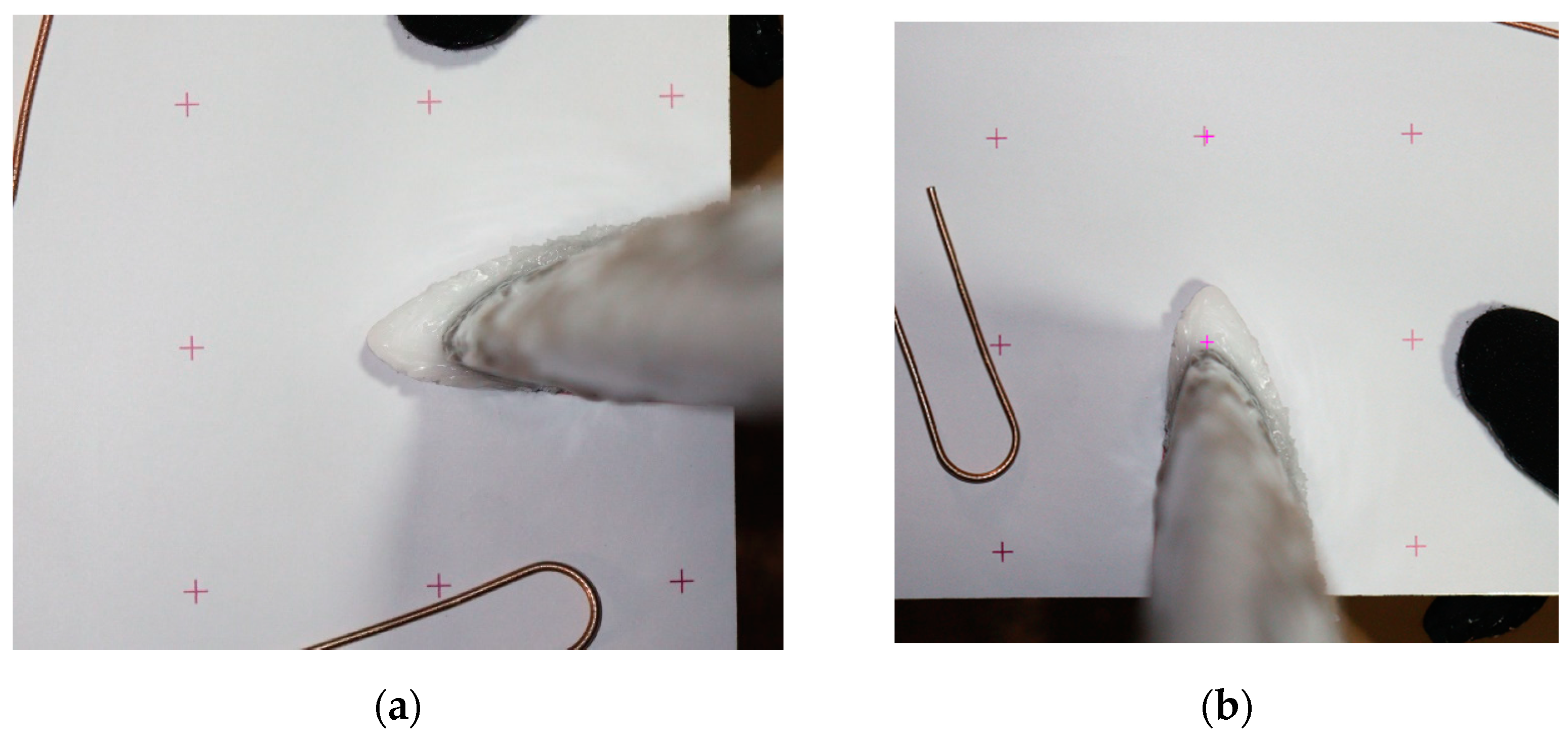
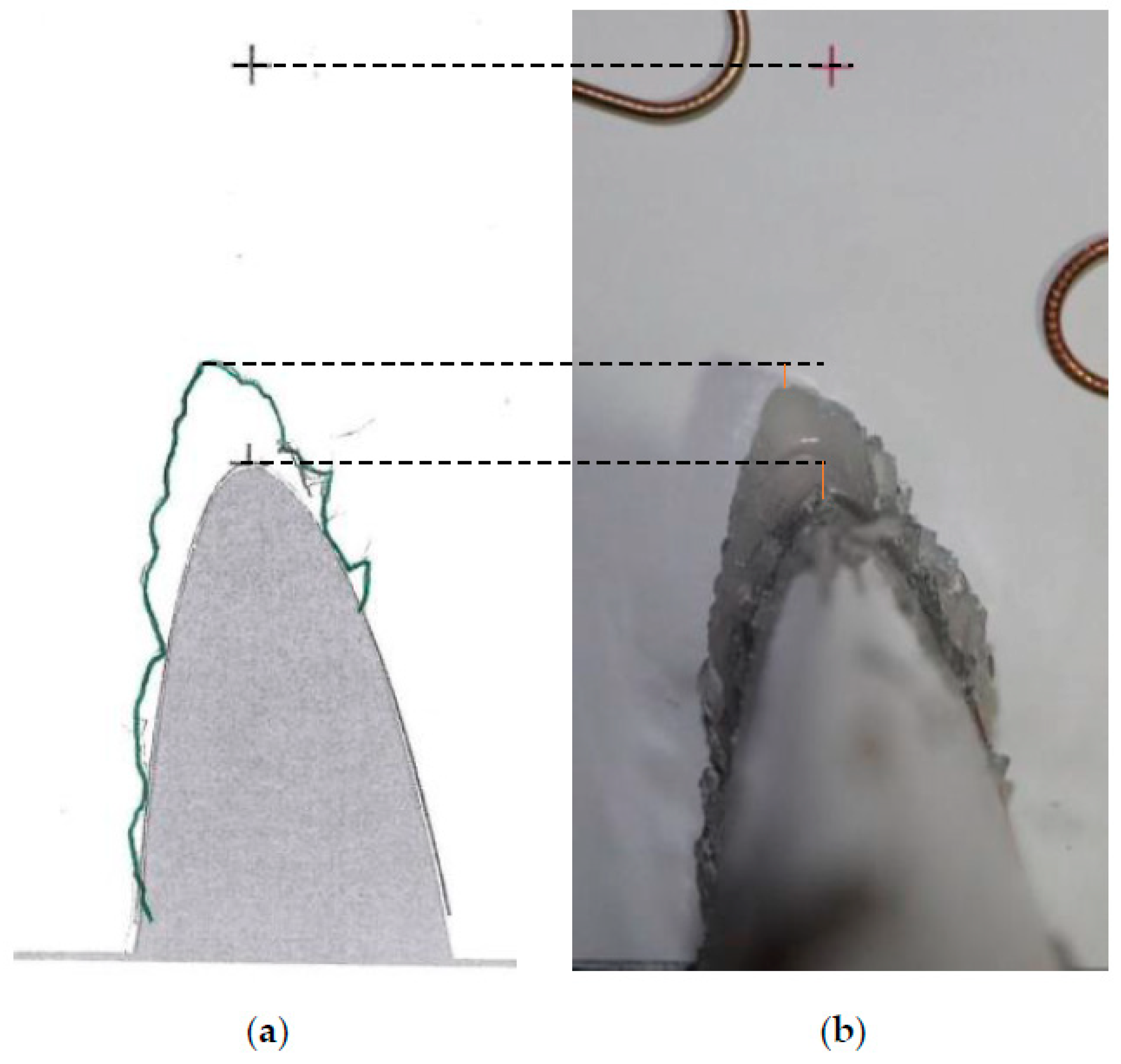
Second, for both techniques, it is essential to have a good alignment of the calibration paper with the leading edge of the airfoil. After taking the ice cuts, it is necessary to check that the supporting background plate and the calibration paper touch the airfoil surface. Two possible errors were observed: either the ice cut was not conducted properly, and the support plate was placed on a thin layer of ice instead of the airfoil surface (usually for glaze ice cases), or the plate was placed in contact with the airfoil, but the calibration paper was not touching the airfoil (this occurs for opaque ice—rime/mixed—where the reference point is not visible through the ice). Both have the same effect and generate lower ice thickness values, as the reference point is placed higher than the leading edge of the airfoil. This error can be identified by comparing the leading-edge thickness results with the caliper measurements. For the IP method, it can also be observed by calculating the position of the reference point based on the network of points on the calibration paper.
The support plate–calibration paper ensemble must be kept in a normal direction to the airfoil’s surface during data acquisition. This practice will avoid projection errors in the ice profiles for both techniques.
The best practices for the image processing method focus mainly on the camera alignment and obtaining a good quality of the initial image. As previously stated, ideally, a trial of the camera position should be conducted in order to position the camera perpendicularly to the calibration plate. To check this alignment, it is important to capture multiple calibration signs in the field of view so as to compare the magnification factor between 2 consecutive points from different regions of the paper. The magnification factor should not show significant variation between regions.
In order to well-capture the suction side and pressure side of the airfoil, the camera should be positioned so as to have a clear view of both parts and avoid blurred regions, but without placing the camera too far from the airfoil. This would decrease the spatial resolution and increase the uncertainty of the ice edge detection. If this is not possible with one picture in some specific setups, two pictures, one for the suction side and one for the pressure side, could be taken and the resulting profiles merged during post-processing. During this process, it is essential to keep the same magnification factor in both images.
In addition to avoiding light reflections or shadows in the image, the quality of the 2D ice profile can be improved by photographing thin ice cuts (as thin as possible below 1 cm). This will limit the capturing of 3D effects in the 2D ice profile. Another way of improving the ice edge detection quality in the images would be the use of colored background paper (preferably dark). This would increase the ice–background contrast and generate higher peaks of the intensity gradients on the ice edge.
The best practices for the scan detection technique focus mainly on generating manual tracings that are as accurate as possible. As the experimenter’s experience is crucial for reducing human error, it is advised that the person who will take the manual ice tracings practices the entire ice profile generation process before the real experiments. It is recommended that the same experimenter takes all of the manual tracings for an experimental campaign. Also, during the initial manual tracing, it is recommended to keep the pencil inclination on the paper constant. This should avoid artificial thickness variation in the ice profile.
Regarding the pre-processing step of redrawing the manual tracing with the green pencil, a sharp pencil should be used in order to avoid additional precision loss and dampening of the ice profile’s features. Moreover, the resolution of the scanner and the printer could produce additional dampening of the ice profile, increasing the measurement uncertainty. Therefore, a high scanner and printer resolution would be beneficial. The accuracy could be improved by scanning the original ice tracing only once and performing all of the following steps on the computer. Ideally, instead of manually re-tracing the original shape in color, a graphic editor would be used to change the tracings’ color in the scanned drawing. This would partially reduce human error, and thus, likely improve the profile accuracy and reduce the amount of post-processing code adjustments. If conducted manually, this step would significantly increase the amount of time required. Automation might be possible, but it would be very difficult, since the code would have to find the correct tracing automatically when multiple lines were drawn during the initial ice tracing process.
These are the best practices and recommendations for maximizing the efficiency and accuracy of the two 2D ice profile measurement techniques. Most of the sources of error are similar for all different icing regimes. Thus, the two methods presented in this paper are expected to perform equally for rime accretions and glaze accretions. For most established techniques, accurately measuring rime ice shapes is easier, because the geometry is typically easier.
Below, a comparison of the techniques with the ones existing in literature is conducted.
The IP technique has a higher accuracy and shorter acquisition and processing time compared to the manual tracing method. Its absolute errors range between −0.4 and +0.7 mm, while, for manual tracing, the absolute error range computed against caliper measurements and reported in Reference [9] is from −1.6 to +2.5 mm. The IP technique is more expensive than manual tracing, as it implies the costs of a camera and a MATLAB license. However, its cost could be reduced by implementing the algorithm in an open-source programming language. Compared to the manual tracing method, the SD technique has a similar absolute error range from −1.2 mm to +2.6 mm. This was expected, as it is based on manual tracing profiles. However, the post-processing time of the SD method is automatic, which reduces human error, is faster, and is less cumbersome than the manual tracing technique, although the SD method is more expensive due to the required MATLAB license.
A direct comparison of the IP method accuracy was not possible for the photogrammetry technique, as no exact accuracy value was found in Reference [9]. However, besides missing the 3D capability, the IP technique is less expensive than photogrammetry because it does not require additional layers of paint/powder. It also has a significantly reduced testing time, mainly because it does not require a drying process. Also, there are fewer images to capture when using the IP method. Compared to photogrammetry, the conclusions for the IP technique are similar to the SD method.
As in the case of photogrammetry, no accuracy values were found for ice accretion measurements using the molding technique. However, based on the techniques’ description provided in Reference [25], good accuracy is reported for molding methods. It is a cumbersome testing process, though, during which, depending on the molds’ material, the tested ice piece might be damaged if not handled carefully. This, combined with the long amount of time needed for the mold material to cure (several hours), makes the IP method faster, cheaper, and simpler to use. However, the IP technique has no 3D capability. The conclusions about the molding versus the IP technique also apply to the comparison of molding with the SD technique.
Compared to the structured light technique [28], which, in the cited study, had a spatial resolution window of 1 × 1 mm and an ice thickness measurement uncertainty of ± 0.04 mm, the IP technique has a higher average absolute error of ~0.26 mm. It might capture steep ice thickness variations better, though, as it generates pointwise results. The IP technique is faster to set up (because it does not require a prior parametric study and uses one camera only), is cheaper, and has a simpler post-processing method. However, the IP technique cannot generate 3D ice profiles or dynamic measurements, as is the case with the technique described in Reference [28]. The SD method has a pointwise average absolute error of ~0.98 mm, which represents a much lower accuracy than the structured light technique, but it has the advantages mentioned for the IP technique. Additionally, both the IP and SD techniques are more versatile than the structured light technique, as they do not require a complex experimental setup or optical access to the IWT’s test section, and they could even be adapted for small-scale field measurements.
Compared to the 3D laser scanning technique presented in Reference [32], which employed a Romer 7530SI scanner with a resolution of 0.05 mm, the IP method has a one-order-of-magnitude lower accuracy (~0.26 mm), and it is not capable of generating 3D ice profiles. Another drawback of the IP technique would be that, in order to generate continuous-line 2D profiles, an ice profile reconstruction step is required, which might further decrease the accuracy in some cases. However, for 2D profiles, it is very low-cost and fast compared to the cumbersome data acquisition and processing described in Reference [32]. Compared to the 3D laser scanning, the SD method has almost two-orders-of-magnitude reduced accuracy (~0.98 mm), it generates only continuous line 2D profiles, it is cheaper, faster, and has a simpler acquisition and post-processing method.
A limitation of both methods presented in this study is that they only generate 2D ice profiles and not 3D profiles. Generating accurate 3D profiles is more valuable, especially for glaze ice, which produces more variation in the spanwise direction. However, even though technological progress allows for more numerical simulations of 3D profiles than in the past, simulating 2D ice shapes is still common [55,56]. Additionally, conducting experiments on the aerodynamic performance in conventional wind tunnels is also not uncommon using 2D ice shapes extruded in the spanwise direction [10,57,58,59].
Regarding the third post-processing technique presented in this paper, the 1D thickness ice profile generator, its applicability could be further developed. The technique allows for a more quantitative ice profile investigation than 2D ice profiles. Section 3.3 presents the proof of concept for the possibility of identifying the ice accretion regimes based on the 1D ice thickness profiles and easier identification of the maximum ice thickness position along the airfoil profile. It is believed that these profiles could also be used for fast estimations of the accumulated ice mass. Further validation of these concepts is necessary, but given the proof of concept, the technique could be a promising tool for estimating the ice accretion regimes together with the angle of attack at which they formed for field tests or after in-flight icing events in which some of the atmospheric conditions might be unknown. This information could be estimated by an examination of the 1D ice thickness profile and might be useful for damage reports, research and development phase of ice protection systems, reverse engineering of atmospheric conditions in case of sensor failure, etc.

5. Conclusions

The aim of this work was to provide two, 2D ice accretion measurement techniques that are low-cost, easily available, have efficient post-processing (automatized algorithms), and offer good accuracy in ice thickness measurements and 2D ice shapes. The ice edge detection image processing method generated ice thickness results with an averaged absolute error of ~0.26 mm and an averaged percentual error of ~2.2%, while, for the manual tracing scan detection method, the average absolute error was ~0.98 mm and the averaged percentual one was ~9.5%. For both techniques, the errors were computed against the ice thickness caliper measurements, and their absolute values were averaged over the 13 ice accretion cases studied, ranging over all ice accretion regimes.
The two 2D ice profile measurement techniques developed, image processing ice edge detection and manual tracing scan detection, were applied to ice accretion data obtained in icing wind tunnel experiments, and they were validated against experimental leading-edge ice thickness measurements.
Both techniques show good accuracy, with an average absolute error lower than 1 mm and an average percentual error lower than 10% for the measured ice thickness and the detected 2D ice shapes. Based on an error and performance analysis, the edge detection image processing resulted as being the optimal technique for high-accuracy ice thickness measurements and high-resolution ice profiling The scan detection technique is optimal to be applied when the 2D ice profiling will be further used for CFD applications, as its continuous line profile makes it suitable for the generation of ice geometries.
The additional post-processing 1D thickness technique can be successfully applied to any 2D ice profiles as long as the airfoil profile is also available. This technique allows for a faster ice thickness analysis and identification of the ice accretion regimes.
The main advantages of the developed ice accretion measurement techniques are that they are inexpensive, readily available, and easy to use, and they provide a reduced post-processing time and good accuracy. Their costs could be further reduced by implementing the post-processing algorithms in an open-source programming language.

Author Contributions

Conceptualization, A.E. and R.H.; methodology, A.E., R.H. and J.W.; software, A.E. and J.W.; validation, A.E. and J.W.; formal analysis, A.E., J.v.B. and P.H.; investigation, A.E., J.W. and R.H.; resources, A.E. and R.H.; data curation, A.E., J.W. and R.H.; writing—original draft preparation, A.E. and J.W.; writing—review and editing, A.E., J.W., R.H., J.v.B. and P.H.; visualization, A.E. and J.W.; supervision, R.H., J.v.B. and P.H.; project administration, R.H. and A.E.; funding acquisition, A.E., J.v.B. and R.H. All authors have read and agreed to the published version of the manuscript.

Funding

This research was funded by the F.R.S.-FNRS mobility funding, grant number 35699386, and by the VKI Alumni Association Research Travel grant. The work was partly sponsored by the Research Council of Norway through the following project codes: 223254, 316425, and 318000. A. Enache was supported by the Belgian F.R.S-FNRS with a FRIA fellowship, grant number 35484427, and by the von Karman Institute for Fluid Dynamics with a PhD fellowship.

Data Availability Statement

Data available upon request.

Acknowledgments

We thank Tuomas Jokela, Mikko Tiihonen, and Timo Karlsson from VTT for their support during the wind tunnel tests.

Conflicts of Interest

The authors declare no conflict of interest.

Appendix A

Figure A1. Interpolation-based reconstructed profiles generated using the IP method for problematic images: (a) run 15—multiple light reflections on the ice formations downstream the leading edge; (b) run 247—regions of shadow near the ice on the leading edge and downstream on the pressure side. Both types of defects generate large gaps in the detected profiles (see Figure 16b and Figure 19b, respectively), which leads to a faulty reconstruction with the interpolation method.
Aerospace 10 00451 g0a1

Appendix B

The fact that, initially, both the ice shape and the airfoil only exist as point clouds increases the complexity of calculating the ice thickness. In order to obtain reasonable thickness values, either the airfoil must be continuous, or the density of the airfoil points must be very large. Otherwise, the thickness would only be calculated between the ice shape points and a few airfoil points, introducing large errors, as can be seen in Figure A7. To keep the calculations simple, the airfoil is assumed to be linear between every airfoil point. Thus, at this point, the algorithm has a cloud of points that make up the ice shape and several linear line segments that make up the airfoil.
Figure A2. Drawing of the idea behind the thickness calculation. Airfoil points are black. The black line shows the airfoil segment of interest, and the dotted black lines show the neighboring airfoil segments. Ice points are shown as asterixis. The blue ice point is closer to the airfoil line than to the endpoints. This also shows the importance of a continuous airfoil line (red vs. blue). The magenta-colored ice point is closer to the endpoint of the line segment of interest than to the line.
Aerospace 10 00451 g0a2
The following calculations were made for each ice shape point separately. First, the minimum distance between the ice shape point and every airfoil segment is calculated. Given that it is only a line segment and not a line, the calculation of the minimum distance consists of more than just a single equation. With this algorithm, the line segment is extended to a line of infinite length. The next step is to use orthogonal projection to project the ice shape point on the line. The distance between the projected point and the real point is the distance between the ice shape point and the line with infinite length.
After calculating the position of the closest point, the algorithm checks the position of this closest point to the line segment. Two cases exist for the position of the closest point. First, the closest point can be between the endpoints of the line segment and thus inside the line segment. In this case, the minimum distance between the ice point and the infinite line is also the minimum distance between the ice point and the line segment. This case is shown in blue in Figure A2. The second case is that the closest point is not between the endpoints of the line segment. Hence, the closest point is outside the line segment. In this case, the minimum distance between the ice point and the line segment is the smaller of the two distances between the ice point and the endpoints of the line segment. This case is shown in magenta in Figure A2.

Appendix C

Figure A3. Leading edge detail of the 1D ice profile of the airfoil’s length (T = −10 °C, rime ice) obtained by converting the 2D profiles generated by the image processing (IP) and the scan detection (SD) techniques for (a) run 166, (b) run 12, and (c) run 44.
Aerospace 10 00451 g0a3
Figure A4. Leading edge detail of the 1D ice profile of the airfoil’s length (T = −20 °C, rime ice) obtained by converting the 2D profiles generated by the image processing (IP) and the scan detection (SD) techniques for (a) run 245 and (b) run 247.
Aerospace 10 00451 g0a4
Figure A5. Leading edge detail of the 1D ice profile of the airfoil’s length (T = −2 °C, glaze ice) obtained by converting the 2D profiles generated by the image processing (IP) and the scan detection (SD) techniques for (a) run 183 and (b) run 199.
Aerospace 10 00451 g0a5
Figure A6. Leading edge detail of the 1D ice profile of the airfoil’s length (T = −4 °C, mixed ice) obtained by converting the 2D profiles generated by the image processing (IP) and the scan detection (SD) techniques for (a) run 14, (b) run 15, and (c) run 23.
Aerospace 10 00451 g0a6
Figure A7. Leading edge detail of the 1D ice profile of the airfoil’s length (T = −5 °C, mixed ice) obtained by converting the 2D profiles generated by the image processing (IP) and the scan detection (SD) techniques for (a) run 110, (b) run 87, and (c) run 231.
Aerospace 10 00451 g0a7

Appendix D

Figure A8. Estimation of measuring paper misalignment for run 231L: (a) the scanned drawing of the ice shape profile, which is the (a) raw data for the SD technique is compared with (b) the experimental image, which is the raw data for the IP technique. Straight interrupted lines mark the drawings’ important features (alignment cross, maximum ice thickness, and LE reference point) and connect them with their image equivalents. The orange segments mark the difference between the LE reference and the maximum ice thickness for both techniques. The observed orange segments’ size, despite the connected alignment crosses, shows the paper’s misalignment for the manual drawing.
Aerospace 10 00451 g0a8

References

  1. Leary, W.M. “We Freeze to Please”: A History of NASA’s Icing Research Tunnel and the Quest for Flight Safety; National Aeronautics and Space Administration: Washington, DC, USA, 2002. Available online: https://history.nasa.gov/sp4226.pdf (accessed on 10 January 2023).
  2. Bragg, M.; Perkins, W.; Sarter, N.; Basar, T.; Voulgaris, P.; Gurbacki, H.; Melody, J.; McCray, S. An interdisciplinary approach to inflight aircraft icing safety. In Proceedings of the 36th AIAA Aerospace Sciences Meeting and Exhibit, Reno, NV, USA, 12–15 January 1998. [Google Scholar] [CrossRef] [Green Version]
  3. Gent, R.W.; Dart, N.P.; Cansdale, J.T. Aircraft icing. Philos. Trans. R. Soc. A Math. Phys. Eng. Sci. 2000, 358, 2873–2911. [Google Scholar] [CrossRef]
  4. Vukis, T. Overview and risk assessment of icing for transport category aircraft and components. In Proceedings of the 40th AIAA Aerospace Sciences Meeting & Exhibit, Reno, NV, USA, 14–17 January 2002. [Google Scholar] [CrossRef]
  5. Bragg, M.; Broeren, A.; Blumenthal, L. Iced-airfoil aerodynamics. Prog. Aerosp. Sci. 2005, 41, 323–362. [Google Scholar] [CrossRef]
  6. Hann, R.; Johansen, T. Unsettled Topics in UAV Icing. SAE Edge Research Report; SAE International: Warrendale, PA, USA, 2020. [Google Scholar]
  7. Cao, Y.; Tan, W.; Wu, Z. Aircraft icing: An ongoing threat to aviation safety. Aerosp. Sci. Technol. 2018, 75, 353–385. [Google Scholar] [CrossRef]
  8. Yamazaki, M.; Jemcov, A.; Sakaue, H. A Review on the Current Status of Icing Physics and Mitigation in Aviation. Aerospace 2021, 8, 188. [Google Scholar] [CrossRef]
  9. Hann, R. UAV Icing: Ice Accretion Experiments and Validation. In Proceedings of the International Conference on Icing of Aircraft, Engines, and Structures, Minneapolis, MN, USA, 17–21 June 2019. [Google Scholar] [CrossRef]
  10. Oswald, J.; Enache, A.; Hann, R.; Glabeke, G.; Lutz, T. UAV Icing: Experimental and Numerical Study of Glaze Ice Performance Penalties on an RG-15 Airfoil. In Proceedings of the AIAA Scitech 2022 Forum, San Diego, CA, USA, 3–7 January 2022. [Google Scholar] [CrossRef]
  11. Lynch, F.T.; Khodadoust, A. Effects of ice accretions on aircraft aerodynamics. Prog. Aerosp. Sci. 2001, 37, 669–767. [Google Scholar] [CrossRef]
  12. Müller, N.; Hann, R. UAV Icing: A Performance Model for a UAV Propeller in Icing Conditions. In Proceedings of the AIAA Aviation 2022 Forum, Chicago, IL, USA, 27 June–1 July 2022. [Google Scholar] [CrossRef]
  13. Yamauchi, G.K. A Summary of NASA Rotary Wing Research: Circa 2008–2018. NASA/TP—2019–220459; NASA Ames Research Center Moffett Field: Mountain View, CA, USA, 2019. [Google Scholar]
  14. Liu, Y.; Li, L.; Chen, W.; Tian, W.; Hu, H. An experimental study on the aerodynamic performance degradation of a UAS propeller model induced by ice accretion process. Exp. Therm. Fluid Sci. 2019, 102, 101–112. [Google Scholar] [CrossRef]
  15. Mason, J.; Chow, P.; Riley, J. Engine Ice Crystal Icing Technology Plan with Research Needs; DOT/FAA/TC-20/34; Federal Aviation Administration, William J. Hughes Technical Center, Atlantic City International Airport: Egg Harbor Township, NJ, USA, 2020.
  16. Struk, P.; Broeren, A.; Potapczuk, M.; Kreeger, R.; Blankenship, K.; Chen, R.-C.; Flege Al Porter, C.; Ratvasky, T.; Van Zante, D.; Van Zante, J.; et al. NASA Analysis of Alternatives Study for Icing Research; NASA/TM-20220006956; NASA Glenn Research Center: Cleveland, OH, USA, 2022.
  17. Yugulis, K.; Chase, D.; McCrink, M. Ice Accretion Analysis for the Development of the HeatCoat Electrothermal Ice Protection System. In Proceedings of the AIAA Aviation 2020 Forum, Online Event, 15–19 June 2020. [Google Scholar] [CrossRef]
  18. Thomas, S.K.; Cassoni, R.P.; MacArthur, C.D. Aircraft anti-icing and de-icing techniques and modeling. J. Aircr. 1996, 33, 841–854. [Google Scholar] [CrossRef]
  19. Hann, R.; Enache, A.; Nielsen, M.C.; Stovner, B.N.; van Beeck, J.; Johansen, T.A.; Borup, K.T. Experimental Heat Loads for Electrothermal Anti-Icing and De-Icing on UAVs. Aerospace 2021, 8, 83. [Google Scholar] [CrossRef]
  20. Moser, R.; Reinholz, B.; Breitfuß, W.; Diebald, S.; Kollmann, P.; Humpel, S.; Puffing, R.; Kozomara, D.; Schweighart, S.; Hassler, W.; et al. Generation of Validation Data for an Electrothermal Ice Protection System. In Proceedings of the AIAA AVIATION 2022 Forum, Chicago, IL, USA, 27 June–1 July 2022. [Google Scholar] [CrossRef]
  21. Hann, R. Atmospheric Ice Accretions, Aerodynamic Icing Penalties, and Ice Protection Systems on Unmanned Aerial Vehicles. Ph.D. Thesis, Norwegian University of Science and Technology, Trondheim, Norway, 2020. Available online: https://ntnuopen.ntnu.no/ntnu-xmlui/handle/11250/2657638 (accessed on 7 May 2023).
  22. Reehorst, A.; Vargas, M.; Hazan, D.; Breuer, K.; Hansman, R. Close-up Analysis of Aircraft Ice Accretion Roughness. In Proceedings of the AIAA 31st Aerospace Sciences Meeting, Reno, NV, USA, 11–14 January 1993. AIAA-93-0029. [Google Scholar]
  23. Potapczuk, M.G.; Reinmann, J.J. Icing Simulation: A Survey of Computer Models and Experimental Facilities. In Proceedings of the 68th AGARD Fluid Dynamics Panel Specialists Meeting, Toulouse, France, 29 April–1 May 1991. [Google Scholar]
  24. Kind, R.J.; Potapczuk, M.G.; Feo, A.; Golia, C.; Shah, A.D. Experimental and computational simulation of in-flight icing phenomena. Prog. Aerosp. Sci. 1998, 34, 257–345. [Google Scholar] [CrossRef]
  25. Reehorst, A.L.; Richter, G.P. New Methods and Materials for Molding and Casting Ice Formations; NASA Technical Memorandum 100126; NASA Lewis Research Center: Cleveland, OH, USA, 1987.
  26. Vannuyen, T. Process Developed for Forming Urethane Ice Models; Technical Report 20050181946; NASA Lewis Research Center: Cleveland, OH, USA, 1998.
  27. Anderson, D.N.; Hentschel, D.B.; Ruff, G.A. Measurement and Correlation of Ice Accretion Roughness; NASA CR—2003-211823, NASA Glenn Research Center: Cleveland, OH, USA, 1998. [Google Scholar]
  28. Zhang, K.; Wei, T.; Hu, H. An experimental investigation on the surface water transport process over an airfoil by using a digital image projection technique. Exp. Fluids 2015, 56, 173. [Google Scholar] [CrossRef]
  29. Veerakumar, R.; Gao, L.; Liu, Y.; Hu, H. Dynamic ice accretion process and its effects on the aerodynamic drag characteristics of a power transmission cable model. Cold Reg. Sci. Technol. 2020, 169, 102908. [Google Scholar] [CrossRef]
  30. Gao, L.; Veerakumar, R.; Liu, Y.; Hu, H. Quantification of the 3D shapes of the ice structures accreted on a wind turbine airfoil model. J. Vis. 2019, 22, 661–667. [Google Scholar] [CrossRef]
  31. Broeren, A.P.; Addy, H.E.J.; Lee, S.; Monastero, M. Validation of 3-D Ice Accretion Measurement Methodology for Experimental Aerodynamic Simulation; NASA/TM—2015-218724; NASA Glenn Research Center: Cleaveland, OH, USA, 2015.
  32. McClain, S.T.; Vargas, M.; Tsao, J.-C.; Broeren, A.P.; Lee, S. Ice Accretion Roughness Measurements and Modeling. In Proceedings of the 7th European Conference For Aeronautics And Space Sciences (Eucass), Milan, Italy, 3–6 July 2017. [Google Scholar] [CrossRef]
  33. Siquig, A. Impact of Icing on Unmanned Aerial Vehicle (UAV) Operations; ADA231191, Naval Environmental Prediction Research Facility: Monterey, CA, USA, 1990. [Google Scholar]
  34. Szilder, K.; McIlwain, S. In-Flight Icing of UAVs—The Influence of Reynolds Number on the Ice Accretion Process. SAE Tech. Pap. 2011, 1, 2572. [Google Scholar] [CrossRef]
  35. Hann, R.; Johansen, T.A. UAV icing: The influence of airspeed and chord length on performance degradation. Aircr. Eng. Aerosp. Technol. 2021, 93, 832–841. [Google Scholar] [CrossRef]
  36. Dastres, R.; Soori, M. Advanced Image Processing Systems. Int. J. Imagining Robot. 2021, 21, 27–44. Available online: https://hal.science/hal-03168963 (accessed on 10 January 2023).
  37. Prabaharan, T.; Periasamy, P.; Mugendiran, V. Ramanan Studies on application of image processing in various fields: An overview. In Proceedings of the IOP Conference Series: Materials Science and Engineering, Chennai, India, 18–23 July 2020. [Google Scholar] [CrossRef]
  38. Mendez, M.; Németh, L.; Buchlin, J.-M. Measurement of Liquid Film Thickness via Light Absorption and Laser Tomography. EPJ Web Conf. 2016, 114, 02072. [Google Scholar] [CrossRef] [Green Version]
  39. Mendez, M.; Scelzo, M.; Buchlin, J.-M. Multiscale modal analysis of an oscillating impinging gas jet. Exp. Therm. Fluid Sci. 2018, 91, 256–276. [Google Scholar] [CrossRef]
  40. Serdyukov, V.; Malakhov, I.; Surtaev, A. High-speed visualization and image processing of sub-atmospheric water boiling on a transparent heater. J. Vis. 2020, 23, 873–884. [Google Scholar] [CrossRef]
  41. Zhong, X.; Dong, J.; Meng, R.; Liu, M.; Pan, X. Quantitative Evaluation of Submerged Cavitation Jet Performance Based on Image Processing Method. J. Mar. Sci. Eng. 2022, 10, 1336. [Google Scholar] [CrossRef]
  42. Joyce, K.E.; Belliss, S.E.; Samsonov, S.V.; McNeill, S.J.; Glassey, P.J. A review of the status of satellite remote sensing and image processing techniques for mapping natural hazards and disasters. Prog. Phys. Geogr. Earth Environ. 2009, 33, 183–207. [Google Scholar] [CrossRef] [Green Version]
  43. Yuan, C.; Liu, Z.; Zhang, Y. Aerial Images-Based Forest Fire Detection for Firefighting Using Optical Remote Sensing Techniques and Unmanned Aerial Vehicles. J. Intell. Robot. Syst. 2017, 88, 635–654. [Google Scholar] [CrossRef]
  44. Jawak, S.; Wankhede, S.; Luis, A.; Balakrishna, K. Impact of Image-Processing Routines on Mapping Glacier Surface Facies from Svalbard and the Himalayas Using Pixel-Based Methods. Remote Sens. 2022, 14, 1414. [Google Scholar] [CrossRef]
  45. Loerke, D.; le Duc, Q.; Blonk, I.; Kerstens, A.; Spanjaard, E.; Machacek, M.; Danuser, G.; de Rooij, J. Quantitative imaging of epithelial cell scattering identifies specific inhibitors of cell motility and cell-cell dissociation. Sci. Signal. 2012, 5, rs5. [Google Scholar] [CrossRef] [Green Version]
  46. Petrellis, N. A Review of Image Processing Techniques Common in Human and Plant Disease Diagnosis. Symmetry 2018, 10, 270. [Google Scholar] [CrossRef] [Green Version]
  47. Argast, G.; Fricker, P. Using Image Processing and Statistical Analysis to Quantify Cell Scattering for Cancer Drug Research; The MathWorks, Inc.: Natick, MA, USA, 2012; Available online: https://es.mathworks.com/company/newsletters/articles/using-image-processing-and-statistical-analysis-to-quantify-cell-scattering-for-cancer-drug-research.html (accessed on 28 February 2023).
  48. Valença, J.; Puente, I.; Júlio, E.; González-Jorge, H.; Arias-Sánchez, P. Assessment of cracks on concrete bridges using image processing supported by laser scanning survey. Constr. Build. Mater. 2017, 146, 668–678. [Google Scholar] [CrossRef]
  49. Deng, L.; Guo, Y.; Chai, B. Defect Detection on a Wind Turbine Blade Based on Digital Image Processing. Processes 2021, 9, 1452. [Google Scholar] [CrossRef]
  50. Al-Bukhaiti, M.A.; Abouel-Kasem, A.; Abdelrhman, Y.; Heshmat, M.; Ahmed, S.M. Image Processing Approach for Estimating the Degree of Surface Eroded by Slurry at Different Impact Velocities. J. Tribol. 2022, 144, 101707. [Google Scholar] [CrossRef]
  51. Tiihonen, M.; Jokela, T.; Makkonen, L.; Bluemink, G. VTT Icing Wind Tunnel 2.0. In Winterwind Conference; VTT Technical Research Centre of Finland Ltd.: Espoo, Finland, 2016. [Google Scholar]
  52. Laurikko, J. Emissions Performance of Current TWC Vehicles at Low Ambient Temperature over FTP and ECE Test Cycles. In International Congress & Exposition; SAE International: Warrendale, PA, USA, 1994. [Google Scholar]
  53. Cober, S.G.; Isaac, G.A. Characterization of Aircraft Icing Environments with Supercooled Large Drops for Application to Commercial Aircraft Certification. J. Appl. Meteorol. Climatol. 2012, 51, 265–284. [Google Scholar] [CrossRef]
  54. Ogretim, E.; Huebsch, W.; Shinn, A. Aircraft Ice Accretion Prediction Based on Neural Networks. J. Aircr. 2006, 43, 233–240. [Google Scholar] [CrossRef]
  55. Laurendeau, E.; Bourgault-Cote, S.; Ozcer, I.; Hann, R.; Radenac, E.; Pueyo, A. Summary from the 1st AIAA Ice Prediction Workshop. In Proceedings of the AIAA AVIATION 2022 Forum, Chicago, IL, USA, 27 June–1 July 2022. [Google Scholar] [CrossRef]
  56. Yirtici, O.; Ozgen, S.; Tuncer, I.H. Predictions of ice formations on wind turbine blades and power production losses due to icing. Wind. Energy 2019, 22, 945–958. [Google Scholar] [CrossRef]
  57. Hann, R.; Hearst, R.J.; Sætran, L.R.; Bracchi, T. Experimental and Numerical Icing Penalties of an S826 Airfoil at Low Reynolds Numbers. Aerospace 2020, 7, 4. [Google Scholar] [CrossRef] [Green Version]
  58. Lee, S.; Broeren, A.; Woodard, B.S.; Lum, C.W.; Smith, T.G. Additional Comparison of Iced Aerodynamic Measurements on a Swept Wing from Two Wind Tunnels. In Proceedings of the International Conference on Icing of Aircraft, Engines and Structures, Minneapolis, MN, USA, 17–21 June 2019. [Google Scholar]
  59. Prasad, G.; Rose, B.R.J. Experimental and Computational study of ice accretion effects on aerodynamic performance. Aircr. Eng. Aerosp. Technol. 2020, 92, 827–836. [Google Scholar] [CrossRef]
Figure 1. Schematic of the icing wind tunnel facility with the airfoil model.
Aerospace 10 00451 g001
Figure 2. Exemplary experimental images of the studied ice accretion regimes: frontal views of the iced airfoil’s leading edge for glaze (a) T = −2 °C, mixed (c) T = −5 °C, and rime (e) T = −10 °C ice, with image samples of the corresponding 2D ice profiles, (b), (d), and (f), respectively.
Aerospace 10 00451 g002
Figure 3. Steps of the ice accretion measurement process: (a) the iced leading edge is cut in several span-wise locations using a heated metallic plate with a negative shape of the airfoil’s leading edge. Using the formed ice cuts—detailed in (b)—caliper measurements of the leading-edge ice thickness are performed (c), followed by the manual tracing of the 2D ice profile (d).
Aerospace 10 00451 g003
Figure 4. Edge detection image processing (IP) method flowchart detailing the main steps to obtaining continuous-line 2D ice profiles. The * marks the optional steps of the process. The ice profile reconstruction is optional and is meant to be used when continuous-line profiles are required. The results presented in Section 3 are generated with only the first three steps of this process.
Aerospace 10 00451 g004
Figure 5. Exemplary image processing (IP) post-processing of a glaze ice accretion case: run 183M (middle cut). The pre-processed original image (a) is post-processed in order to obtain the 2D ice profile shown in (b), where the main results are illustrated: the detected profile (in black) of the IP ice edge, the reconstructed (Interp.) ice profile (green), the airfoil profile (red line), and the leading-edge (LE) ice thickness measurement (biggest red cross). The post-processing steps are presented in Figure 6.
Aerospace 10 00451 g005
Figure 6. Illustration of the major steps of the image processing ice edge detection algorithm for glaze ice accretion: (a) image cropped to ROI and signaling the LE reference point, (b) raw detected profile, (c) detection formulation in binary matrix form, (d) filtered final matrix form, (e) verification step (overlapping of the filtered profile with the original image), and (f) airfoil profile reconstructed from user input points. Post-processing of run 183M (middle cut).
Aerospace 10 00451 g006
Figure 7. Exemplary rime ice accretion case—run 245L (left cut). The ice opacity in the pre-processed original image (a) blocks optical access to the leading-edge reference cross; therefore, an additional post-processing feature is used to predict its position based on the position of the nearing signs (sides and top). The final predicted position of the LE reference is shown in (b).
Aerospace 10 00451 g007
Figure 8. Illustration of the major steps of the image processing ice edge detection algorithm for rime ice accretion: (a) image cropped to ROI and signal the predicted position of the LE reference point, (b) raw detected profile, (c) detection formulation in binary matrix form, (d) filtered final matrix form, (e) verification step (overlapping of the filtered profile with the original image), and (f) reconstructed airfoil profile from user input points. Post-processing of run 245L (left cut).
Aerospace 10 00451 g008
Figure 9. Exemplary image processing (IP) post-processing-generated results for rime ice accretion, run 245L (left cut): illustrations of the obtained 2D IP ice edge detected profile (in black), the reconstructed (Interp.) ice profile (green), the airfoil profile (red line), and the leading-edge (LE) ice thickness measurement (biggest red cross). The airfoil input crosses are the points signaled by the user as airfoil limits, while the LE reference is the one predicted by the algorithm in the additional step; these are used in cases of high-opacity ice (as shown in Figure 7b). The post-processing steps are illustrated in Figure 8.
Aerospace 10 00451 g009
Figure 10. Manual drawings scan detection (SD) method flowchart. Main steps to obtaining continuous line 2D ice profiles.
Aerospace 10 00451 g010
Figure 11. The template for the manual ice tracings (a) and an exemplary manual ice tracing (b).
Aerospace 10 00451 g011
Figure 12. The ice shape traced with a green pencil (a) and a comparison between the original manual ice tracing (grey line) and the detected ice shape (dotted blue line) confirming the good match (b).
Aerospace 10 00451 g012
Figure 20. 1D ice profile along the airfoil’s length (T = −10 °C, rime ice), obtained by converting the 2D profiles generated by the image processing (IP) and the scan detection (SD) techniques, for (a) run 166, (b) run 12, and (c) run 44.
Aerospace 10 00451 g020
Figure 21. 1D ice profile along the airfoil’s length (T = −20 °C, rime ice), obtained by converting the 2D profiles generated by the image processing (IP) and the scan detection (SD) techniques, for (a) run 245 and (b) run 247.
Aerospace 10 00451 g021
Figure 22. 1D ice profile along the airfoil’s length (T = −2 °C, glaze ice), obtained by converting the 2D profiles generated by the image processing (IP) and the scan detection (SD) techniques, for (a) run 183 and (b) run 199.
Aerospace 10 00451 g022
Figure 23. 1D ice profile along the airfoil’s length (T = −4 °C, mixed ice), obtained by converting the 2D profiles generated by the image processing (IP) and the scan detection (SD) techniques, for (a) run 14, (b) run 15, and (c) run 23.
Aerospace 10 00451 g023
Figure 24. 1D ice profile along the airfoil’s length (T = −5 °C, mixed ice), obtained by converting the 2D profiles generated by the image processing (IP) and the scan detection (SD) techniques, for (a) run 110, (b) run 87, and (c) run 231.
Aerospace 10 00451 g024
Figure 25. Leading edge detail of the 1D ice profile along the airfoil’s length for run 231, obtained by con-verting the 2D profiles generated by the image processing (IP) and the scan detection (SD) techniques.
Aerospace 10 00451 g025
Table 1. Dimensions of the tested airfoil models.
IDAirfoil ProfileChord [m]Span [m]
1RG-150.450.65
2RG-150.300.65
3SD80200.250.65
Table 2. Ice accretion experimental testing conditions.
Parameters
Velocity [m/s]25
Temperature [°C]−2, −4, −5, −10, −20
Reynolds number, Re [–]~9 × 10⁵
Ice accretion time [min]8, 20
Liquid water content, LWC [g/m3]0.44
Droplet diameter, MVD [µm]24
Angle of attack, AOA [°]0, 8
Table 3. Ice accretion cases—testing conditions and leading-edge ice thickness results—comparison between the experimental (caliper) measurements, the image processing (IP) algorithm results, and the scan detection (SD) results.
Nb.CaseTemperature [°C]Accretion Time [min]Airfoil IDAOA
[°]
Experimental Ice Thickness [mm]IP Ice Thickness [mm]Error IP [%]SD Ice Thickness [mm]Error SD [%]
1‘183M’−220108.107.991.47.0612.8
2‘199M’−220307.907.751.97.317.5
3‘14M’−4202011.8412.27−3.612.20−3.0
4‘15M’−4202012.1711.763.411.416.2
5‘23M’−4201011.0010.851.411.66−6.0
6‘87M’−5202012.8712.96−0.712.810.5
7‘110′−58105.004.931.46.17−23.4
8‘231L’−5201810.9010.761.38.3423.5
9‘166L’−10201013.0012.722.211.2813.2
10‘12M’−10202013.2012.832.810.7918.3
11‘44R’−10202012.7012.372.612.96−2.0
12‘245L’−20201012.1011.405.811.455.4
13‘247M’−20203013.1013.070.213.25−1.1
Average errors for:IP0.26 [mm]2.2 [%]SD0.98 [mm]9.5 [%]
Disclaimer/Publisher’s Note: The statements, opinions and data contained in all publications are solely those of the individual author(s) and contributor(s) and not of MDPI and/or the editor(s). MDPI and/or the editor(s) disclaim responsibility for any injury to people or property resulting from any ideas, methods, instructions or products referred to in the content.

