Aeroengine Diagnosis Using a New Robust Gradient-like Methodology

Abstract

A new gradient-like methodology has been developed for aeroengine diagnosis, determining the engine health condition, which is defined by the engine degradation from an undegraded state and uses measurements at various sensors distributed along the engine. The developed tools are able to accurately compute, not only the engine degradation, but also the turbine inlet temperature, which is very important and novel in the field. The quality of a given sensors set is evaluated, and a method is developed to guide in the improvement of deficient sensors sets. The methodology is tested in a representative two-spool turbofan engine, obtaining consistent results in a computationally inexpensive way. Moreover, results are robust in connection with the random noise added to the sensors data.

1. Introduction

Like many other complex systems, aeroengines require maintenance to ensure their good functioning during operation. The current maintenance paradigm is predictive maintenance [1] (also called condition-based maintenance), in which possible failures are anticipated before an expensive or dangerous breakdown occurs. This reduces operational and maintenance costs, including fuel consumption, and increases safety, which is crucial in the aerospace industry. Concerning cost [2], maintenance represents 4% of the total operational cost of typical airlines, while fuel consumption amounts to 33%. Moreover, predictive maintenance is increasingly used in other sectors, such as in the manufacturing [3] and railway [4] industries.

Using measurements in some sensors, failures are anticipated by performing diagnosis [5], namely by monitoring the engine health condition by providing the engine degradation (defined by several degradation parameters) from a baseline (undegraded) state. Once the engine deterioration has been assessed, it is possible to address the prognosis [6,7], namely to identify which actions should be taken to optimize the future operation of the engine.

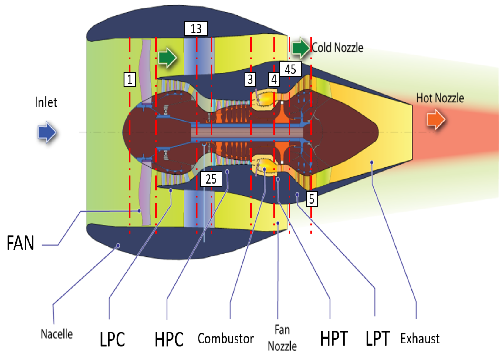
Although the methods developed in the paper apply to other aeroengines (in fact, to more general systems), results will be illustrated considering a representative aeroengine for commercial aviation, namely a CFM56 engine. This is a two-spool turbofan engine, similar to those widely used in commercial aviation nowadays [8]. As sketched in Figure 1, the engine contains a low-pressure spool and a high-pressure spool, which rotate concentrically at different speeds. The mechanically connected (by the high-pressure spool) high-pressure compressor (HPC) and high-pressure turbine (HPT), together with the combustor, constitute the high-pressure part of the engine, or the core engine. The low-pressure part of the engine, namely the fan, the low-pressure compressor (LPC), and the low-pressure turbine (LPT), are also mechanically connected by the low-pressure spool. Sensors can be placed in these components of the engine, which in turn are characterized by several degradation parameters. Some of these can be used for diagnosis, noting that their deviation from the baseline values measure the engine degradation. There is consensus in the literature on the most convenient degradation parameters (mainly, adiabatic efficiencies and flow capacities), after the seminal work by Stamatis et al. [9].

Current aeroengine diagnosis methods can be classified as data-driven or model-based [11,12], although some interesting hybrid methods have been recently developed, such as the physics-informed neural networks [13].

Data-driven methods are usually based on machine learning (via, e.g., neural networks) and statistical algorithms. In particular, it is worth mentioning Bayesian networks [14] and Latent Semantic Analysis [15]. The main drawback of these methods is the required offline computational time, since a very computationally expensive training of the tool is needed, using former experience on failures in the type of engine that is being analyzed. Moreover, training in a given (usually sharp) operational regime range must be repeated to cover other ranges as well. The main advantage is that their online operation is usually fairly fast.

The training stage is avoided in model-based (also called physics-based) methods, which are more flexible and precise. This is because these methods take the underlying physics into account by using a (generally nonlinear) model for the engine operation. Such an engine model computes the sensors outputs in terms of the operational regime and the degradation parameters. It is constructed using both semi-empirical formulae (∼800 algebraic equations) and discrete empirical data, which come in the form of maps from actual measurements (obtained from tests) in the main components of the engine, namely the fan, the low and high pressure compressors and turbines, et cetera. For each engine component, the empirical map covers only a (generally non-rectangular) portion of the operational regime, namely the operational region where data have been acquired. In this work, model outcomes in this section will be called acceptable outcomes, while the remaining outcomes will be referred to as non-acceptable, since the engine model does not simulate the engine operation there well. Discarding non-acceptable model outcomes, model-based diagnosis will be performed in this work by appropriately fitting the sensors outcomes with their counterparts computed by the engine model.

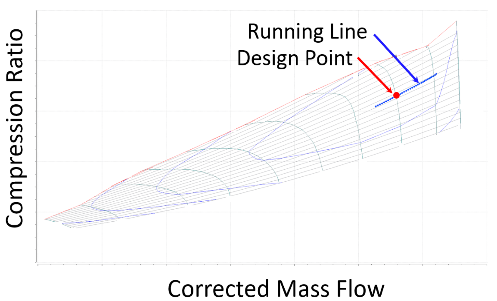
The main turbofan manufactures, such as General Electric, Pratt & Whitney, Rolls-Royce, and Snecma, have developed their own (specifically tailored) engine models, but unfortunately, these models are confidential and not available in the literature. Thus, instead, we shall use an engine model developed with PROOSIS [16], which is a commercial software package that computes the response of the aeroengine using an iterative Powell hybrid method, which is a direct search method [17] able to deal with discrete entries. Such discrete entries are the aforementioned discrete empirical data. A representative empirical map (for the HPC) used by PROOSIS is given in Figure 2, where both the design point where the engine model has been calibrated, and an example of the running line of HPC states reached in a particular engine model operation, are indicated. Points outside this non-rectangular map are unphysical, but can be reached in the outcomes of the engine model along the various iterations of the iterative methods described below, especially for actual engine operational points associated with HPC states close to the boundary of the empirical map. Unphysical solutions of the engine model that are outside the empirical maps, for at least one engine component, are the above mentioned non-acceptable model outcomes.

Among the existing model-based methods to perform aeroengine diagnosis, gas path analysis (GPA) has become increasingly popular after the seminal work by Urban [18]. Earlier GPA methods relied on the assumption that the sensors data depend linearly on the degradation parameters, which is very restrictive. Later, nonlinear GPA methods were developed [9,19] and improved in connection with the required computational time [20] and the role of nonlinearity [21]. In these methods, the linear approximation is replaced by a fixed truncated Taylor expansion around a known baseline state. Thus, these methods provide good results only for somewhat small degradations (around the known state), such that the truncated Taylor approximation is accurate. More recently, GPA has evolved to more efficient methods, some of which sequentially diagnose each turbomaquinery component independently [22] and include transient effects [23]. Others combine GPA itself with other ingredients. For instance, GPA has been combined with genetic algorithms [24,25], which obviously increases the computational cost but also increases the robustness against the sensor noise and bias. The combination of GPA with Kalman filters [26,27], artificial neural networks [28], and Neuro-Fuzzy Inference Systems [29] has also been performed.

The methodology developed in this paper involves two advantages that are novel in the field. First, our iterative methods are able to produce robust, consistent results considering large degradations, for which the fixed truncated Taylor approximation inherent in GPA cannot provide good results. The reason for this is that our methods use an adapted, truncated approximation in each iteration; such approximation improves along iterations until a convergence is achieved. Secondly, we shall compute, not only the degradation parameters, but also the value of the turbine inlet temperature, $T_{4t}$, at which the sensors data have been acquired. Note, according to Figure 1, that this temperature can also be considered as the combustor outlet temperature.

In connection with the joint computation of the degradations and the turbine inlet temperature, it is important to note that, from the engine modeling standpoint, the outcomes (sensors measurements) depend on the degradation of the engine and two degrees of freedom: the flight condition and the operating regime. The flight condition (altitude and Mach number) can be obtained from on-wing measurements and, therefore, will be assumed as known for this study. The operating regime, instead, is a parameter of the utmost importance.

To control the engine regime, a handle parameter is needed in principle. In this regard, different manufacturers make use of different handles, such as the exhaust gas temperature, the engine pressure ratio, or the low-pressure shaft rotational speed. However, from a modeling perspective, the most convenient engine handle is the combustor outlet temperature, $T_{4t}$. This represents the maximum temperature of the thermodynamic cycle, and thus is the parameter that carries the most relevant information about said cycle. Using $T_{4t}$ as an engine handle in commercial aviation is typically avoided, because the high temperatures at the combustor outlet are impractical to measure (thermocouples are not well suited for these environments, and other options such as pyrometers are economically unfeasible for civil aviation). However, conceptually, there is no reason not to use $T_{4t}$ as a handle. In fact, as anticipated, we shall consider this engine handle as an unknown value, along with the degradations, in our diagnosis tool. This means that, in the end, since $T_{4t}$ will be computed, our tool will work without an engine handle. Indeed, the operating regime of the engine will be unknown, and computed as a part of the solution to the diagnosis problem itself. Instead of considering the operating regime as an input to the engine, and assess the deviations from the expected model outputs due to degradations, we have chosen to solve for both the degradations and the operating regime at the same time, as we try to find the combination of $T_{4t}$ and degradations that is compatible (or more likely) with the sensors measurements. Rather than tailoring a tool to exploit a particular set of sensors, our diagnosis approach intends to be able to tackle problems in which sensors can be added (or removed) seamlessly. Note that nothing is taken for granted, not even the engine handle is known a priori. Instead, we shall only use the information (we will ascertain whether this is enough to actually solve the diagnosis problem) coming from the sensors measurements.

Our approach is essentially new in the field. In a different spirit, not solving the inverse problem per se but relying on updating certain ‘tuning parameters’, the in-flight estimation of $T_{4t}$ from sensor measurements has been addressed using piece-wise linear Kalman filters combined with engine models [30,31,32] and hybrid Wiener models [33], focusing on transient behavior. In these works, $T_{4t}$ is estimated using, not only measurements provided by the engine sensors, but also a known control handle from the engine. On the other hand, the computation of $T_{4t}$ is somewhat common practice in aeroengines test benches. The present paper, instead, will provide a very precise and robust in-flight computation of $T_{4t}$, allowing for strong engine degradations.

Another important temperature is the turbine outlet temperature, $T_{5t}$, which is strongly correlated with $T_{4t}$ in healthy conditions and, in fact, has been traditionally used in diagnosis studies to evaluate the engine deterioration. This is because, as $T_{5t}$ increases, for given values of the remaining engine parameters, the engine efficiency decreases and fuel consumption increases. However, this lower temperature cannot substitute $T_{4t}$ in the context of this paper. A sensor measuring $T_{5t}$ will be included. This can be seen in

Table 1. Degradations (x) and sensors (y) descriptions, and average values of the sensor outcomes using the default set of sensors (defined below) for the specific aeroengine formulation considered in Section 4.

Degradations—Description	Sensors—Description	Sensors—Average Values
$x\left(1\right)$–FAN efficiency ${\eta }_{FAN}$	$y\left(1\right)$–$P_{13t}$	$y^{\mathrm{aver}.}\left(1\right)=5.792·{10}^4$ Pa
$x\left(2\right)$– FAN flow capacity ${\mathrm{\Gamma }}_{FAN}$	$y\left(2\right)$–$P_{25t}$	$y^{\mathrm{aver}.}\left(2\right)=1.913·{10}^5$ Pa
$x\left(3\right)$–HPC efficiency ${\eta }_{HPC}$	$y\left(3\right)$–$P_{3t}$	$y^{\mathrm{aver}.}\left(3\right)=1.322·{10}^6$ Pa
$x\left(4\right)$–HPC flow capacity ${\mathrm{\Gamma }}_{HPC}$	$y\left(4\right)$–$T_{25t}$	$y^{\mathrm{aver}.}\left(4\right)=4.302·{10}^2$ K
$x\left(5\right)$–LPC efficiency ${\eta }_{LPC}$	$y\left(5\right)$–$T_{3t}$	$y^{\mathrm{aver}.}\left(5\right)=7.751·{10}^2$ K
$x\left(6\right)$–LPC flow capacity ${\mathrm{\Gamma }}_{LPC}$	$y\left(6\right)$–$T_{45t}$	$y^{\mathrm{aver}.}\left(6\right)=1.111·{10}^3$ K
$x\left(7\right)$–HPT efficiency ${\eta }_{HPT}$	$y\left(7\right)$–$T_{5t}$	$y^{\mathrm{aver}.}\left(7\right)=7.464·{10}^2$ K
$x\left(8\right)$–HPT flow capacity ${\mathrm{\Gamma }}_{HPT}$	$y\left(8\right)$–$N_H$	$y^{\mathrm{aver}.}\left(8\right)=1.031·{10}^4$ rpm
$x\left(9\right)$–LPT efficiency ${\eta }_{LPT}$	$y\left(9\right)$–$N_L$	$y^{\mathrm{aver}.}\left(9\right)=4.141·{10}^3$ rpm
$x\left(10\right)$–LPT flow capacity ${\mathrm{\Gamma }}_{LPT}$	$y\left(10\right)$–$W_F$	$y^{\mathrm{aver}.}\left(10\right)=1.097$ kg/s

, which gives the description of the sensors and degradation parameters (to be thoroughly used and commented in Section 4).

Mathematically, the diagnosis problem could be considered as an inverse problem. This concept is the contrary of the direct problem, which in the present context means computing the sensors data (using the engine model) for a given operational regime and a given set of engine degradations. Inverse problems can be quite ill-conditioned. A well-conditioned formulation of the present inverse problem will be obtained by improving the sensors set.

Anticipating the model-based strategy that will be followed in this work, two types of methods will be developed. In both cases, the ‘correct’ degradations will be obtained by matching measured and computed (using the engine model for varying values of the degradations) sensor data. In the first type of method, (i) appropriate, iterative gradient-like MATLAB software will be used to minimize the root mean square (RMS) difference between measured and computed sensors data. In the second type of method, (ii) a conveniently adapted Newton method, able to cope with constraints and discard non-acceptable outcomes of the engine model, will be developed and used to solve the set of equations that result from equating the measured and computed sensors data. A very preliminary step using the strategy (i) was presented by the authors in [34], but the resolution of the inverse problem was not robust enough and required computing a quite large number of cases. These took several CPU hours in a standard PC, with a microprocessor Intel Core i7-3770 at 3.4 GHz, with 16 GB RAM memory. With this PC, very robust, accurate results will be obtained in the present paper in ∼1.5 CPU minutes and ∼10 CPU seconds, using appropriate versions of the above mentioned strategies (i) and (ii), respectively. Moreover, our methods are transparent to both the particular aeroengine and the particular model that is used to compute the engine performance.

It is interesting to anticipate that, applying the strategy (i), the minimum of the objective function will turn out to be unique (irrespectively of the tunable parameters of the minimization software) for the current diagnosis problem. In fact, for this problem, the uniqueness can be proven for very small degradations because, in this case, the objective function turns out to be convex [35,36]. However, it will be repeatedly tested below that the solution is also unique for non-small degradations and, moreover, the uniqueness of the diagnosis problem will be tested using the strategy (ii) too.

The quality of the sensors data is very important. Albeit sensors precision, the nature of the measured data is crucial. Obviously, the more uncorrelated the available data, the better in connection with the results of the obtained diagnosis. A particular set of sensors, called in this paper the default set of sensors (described in Table 1) will be observed to provide deficient diagnosis results. This is consistent with related difficulties already found in diagnosis studies [37] based on this default set of sensors. Such a set of sensors will be evaluated by a suitable use of truncated singular value decomposition (SVD) [38]. This analysis (which is generic and can be applied to other sensor sets) will also indicate how the default sensors set should be modified to improve diagnosis. It is important to note that choosing convenient sets of sensors, avoiding to increase the number of sensors too much, requires one to assess the quality of the sensors, discarding spurious correlations.

This methodological paper aims at understanding the basics of performing aeroengine diagnosis in an efficient way. In order to facilitate replicating the presented results, the various tools needed for the practical implementation of the methodology will be described in some detail, and precise quantitative results will be given in the form of tables. Even though the goal is to compute $T_{4t}$ along with the degradations, a comparison with previous approaches (in which $T_{4t}$ was not calculated) will require one to also consider the case in which $T_{4t}$ is known. On the other hand, the outcomes of actual sensors mounted in an actual engine are noisy. In order to take this into account, some small random noise with zero mean will be added to the engine model outcomes, concluding that the developed tools are robust in connection with noise.

With the above in mind, the remainder of this paper is organized as follows. The basic data processing tool needed in the analysis, truncated SVD, will be recalled in Section 2, with just enough detail to facilitate its use throughout the paper. The diagnosis methodology will be presented in Section 3. This methodology will be applied using the above-mentioned default set of sensors in Section 4, where the obtained results will be analyzed. Such analysis will indicate how this set of sensors can be improved. Using the improved sensors set, new diagnosis results will be obtained in Section 5 that are dramatically better in connection with computational efficiency, accuracy, and robustness. Finally, some concluding remarks will be addressed in Section 6.

2. Basic Data Processing Tool: Truncated SVD

A very brief account of this well known decomposition is given here, considering the version of SVD implemented in the MATLAB command ‘svd’, option ‘econ’. For a real, generally rectangular, $I\times J$ matrix $\mathbf{A}$, its SVD is given by [38]

$$\mathbf{A}=\mathbf{U}\mathbf{S}{\mathbf{V}}^{\top }\mathrm{or}{A}_{ij}=\sum _{q=1}^Q{s}_q{U}_{iq}{V}_{jq},$$

(1)

where the superscript ${}^{\top }$ denotes the transpose. $\mathbf{U}$ and $\mathbf{V}$ are $I\times Q$ and $J\times Q$ matrices, respectively, with $Q=min\{I,J\}$, such that

$${\mathbf{U}}^{\top }\mathbf{U}={\mathbf{V}}^{\top }\mathbf{V}=I_{Q\times Q},$$

(2)

where $I_{Q\times Q}$ denotes the $Q\times Q$ unit matrix. The elements of the diagonal matrix $\mathbf{S}$ are the singular values, sorted as $s_1\ge s_2\ge \dots \ge s_Q\ge 0$. According to (1), if the last $Q-\tilde{Q}>0$ singular values are quite small (or zero), then neglecting the associated terms in (1), a good truncated approximation of the elements of $\mathbf{A}$, ${\mathbf{A}}^{\mathrm{trunc}.}$, is obtained. Namely,

$$A_{ij}\simeq A_{ij}^{\mathrm{trunc}.}=\sum _{q=1}^{\tilde{Q}}{s}_q{U}_{iq}{V}_{jq}.$$

(3)

It is interesting to note that, multiplying (3) by $V_{j{q}^{\prime }}$ and adding in j, the following $Q-\tilde{Q}$ exact correlations among the columns of ${\mathbf{A}}^{\mathrm{trunc}.}$ are obtained

$$\sum _{j=1}^J{A}_{ij}^{\mathrm{trunc}.}{V}_{j{q}^{\prime }}=\sum _{q=1}^{\tilde{Q}}{s}_q{U}_{iq}\sum _{j=1}^J{V}_{jq}{V}_{j{q}^{\prime }}=0\mathrm{for}i=1,\dots ,I,\tilde{Q}<q^{\prime }\le Q,$$

(4)

where we have taken into account that, according to (2), since $q\le \tilde{Q}$ is different from $q^{\prime }>\tilde{Q}$, we have ${\sum }_{j=1}^J{V}_{jq}{V}_{j{q}^{\prime }}=0$. If the neglected singular values are quite small, then $\mathbf{A}\simeq {\mathbf{A}}^{\mathrm{trunc}.}$ and the exact correlations (4) for ${\mathbf{A}}^{\mathrm{trunc}.}$ are converted into the following approximate correlations among the columns of the matrix $\mathbf{A}$

$$\sum _{j=1}^J{A}_{ij}{V}_{j{q}^{\prime }}\simeq 0\mathrm{for}i=1,\dots ,I\mathrm{and}\tilde{Q}<q^{\prime }\le Q.$$

(5)

SVD also permits for calculating the condition number of the matrix $\mathbf{A}$, as the ratio of the largest singular value of $\mathbf{A}$ to the smallest, which can be directly computed using the MATLAB command ‘cond’. It indicates the accuracy of the results obtained when solving linear systems whose coefficient matrix is $\mathbf{A}$; such accuracy worsens as the condition number increases.

3. Diagnosis Methodology

As anticipated, the aim is to obtain the aeroengine status, defined by a degradations vector $\mathbf{x}$ of size $N_{\mathrm{degrads}}$, using a set of sensors data. Each component of $\mathbf{x}$ shows how much a relevant property of the engine has degraded, and will be defined in %, which gives an automatic scaling of the degradations. Concerning the sensors data, they will be collected in a sensors vector $\mathbf{y}$ of size $N_{\mathrm{sensors}}$. The components of this vector typically give properties such as pressures (measured in Pa), temperatures (in K), rotational speeds (in rpm), and the mass flow rate (in kg/s). As can be observed in Table 1, these components differ among each other by several orders of magnitude, which would worsen the performance of the methodology. Thus, sensors data need to be scaled in such a way that the new values and the range in which they vary are comparable for all sensors. The flight altitude and Mach number are usually given accurately enough by the engine instrumentation and thus can be assumed as known. In the present application, they will be taken as equal to 35,000 feet and 0.8, respectively. These are typical values in cruise conditions, which cover most of the engine operation lifetime.

For a given set of scaled (see Section 4.1 below) sensor measurements, collected in a vector ${\mathbf{y}}^{\mathrm{measur}.}$, we consider the system of equations

$$\mathbf{F}(T_{4t},\mathbf{x})={\mathbf{y}}^{\mathrm{measur}.}.$$

(6)

The left-hand side of this equation represents the direct problem, solved by the engine model as

$$\mathbf{y}=\mathbf{F}(T_{4t},\mathbf{x}).$$

(7)

When $T_{4t}$ is to be computed along with the degradations, it is considered as an unknown in (6), which increases the number of scalar unknowns by one.

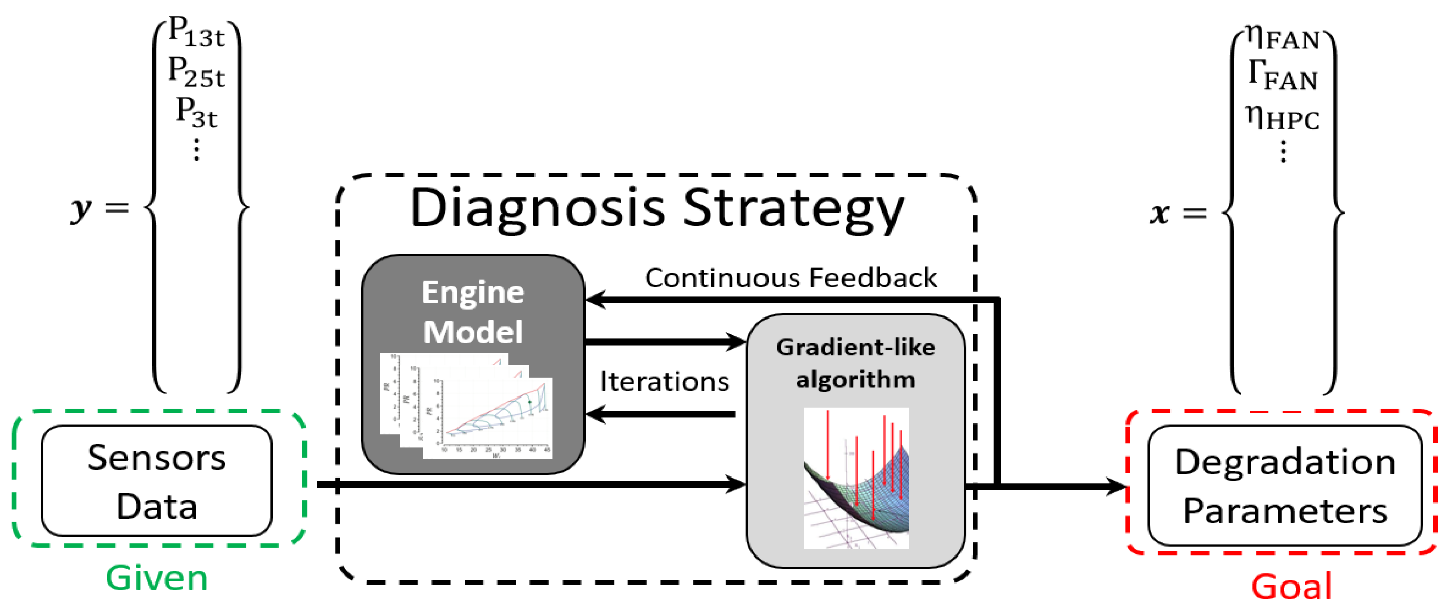
The iterative diagnosis procedure is anticipated in Figure 3, where the indicated gradient-like algorithm will be constructed following one of the two strategies that were anticipated in Section 1 and are detailed now.

A first gradient-like strategy, frequently used to solve inverse problems [39], consists in replacing (6) by an optimization problem, in which either $\mathbf{x}$ alone or the pair $(T_{4t},\mathbf{x})$ are computed by solving the minimization problem

$$\min {∥\mathbf{F}(T_{4t},\mathbf{x})-{\mathbf{y}}^{\mathrm{measur}.}∥}_2,$$

(8)

where ${\parallel ·\parallel }_2$ is the usual Euclidean norm. The associated Jacobian can be very ill-conditioned, and made better conditioned by using a larger number of sensors data, as already conducted in [40] for an inverse problem arising in acoustics. In the present work, the number of available data will be increased (and the condition number of the Hessian decreased) by taking measurements at more than one value of $T_{4t}$ (see below). Moreover, some constraints must be imposed in both formulations, (6) and (8), since, e.g., all degradations must be non-negative (because the engine is degraded, not upgraded) and it is convenient to impose that $T_{4t}$ be in an appropriate range if this temperature is considered as an unknown. In the present work, we shall require that $T_{4t}$ be in a range of $\pm 50$ K around its estimated value provided by the engine instrumentation. This range more than covers the accuracy of the engine instrumentation.

A good constraint optimization method to solve (8) is implemented in the MATLAB function ‘sequential quadratic programming’ (SQP) [41], which is an iterative active-set descend method based on the BFGS algorithm [35].

As a second gradient-like strategy, the formulation (6) will be addressed via an adapted Newton method, able to take constraints into account and to discard non-acceptable engine model outcomes. This method will be described in detail in Section 4.4, when used for the first time.

4. Diagnosis Using Data from the Default Sensors Set

The default set of sensors, described in Table 1—second column, provides measurements of ten properties sketched in Figure 1: $P_{13t}$ (total pressure at FAN exhaust duct), $P_{25t}$ (total pressure in between LPC and HPC), $P_{3t}$ (total pressure at HPC outlet), $T_{25t}$ (temperature in between LPC and HPC), $T_{3t}$ (HPC outlet temperature), $T_{45t}$ (temperature in between LPT and HPT), $T_{5t}$ (LPT outlet temperature), $N_H$ and $N_L$ (rotational speeds of the high and low pressure spools, respectively), and $W_F$ (fuel consumption). The averaged dimensional values of these properties, given in the third column, take very disparate values, as anticipated, and thus they need to be appropriately scaled. Scaling is very computational inexpensive and needs to be performed using the engine model just once, at the outset of the diagnosis process. Once performed, it can be used in all diagnosis studies for the specific engine, for any values of $T_{4t}$ and the degradation parameters.

4.1. Scaling of the Sensors Data

To begin with the scaling of the sensors data for the particular aeroengine that is being diagnosed, the direct problem is simulated using the engine model at the baseline (undegraded) state, for 17 equispaced values of $T_{4t}$ in the range from 1300 K to 1650 K. This range more than covers the values of $T_{4t}$ in cruise conditions (which is ∼1400 K). A degraded engine could be considered, obtaining similar results, as checked below. Then, the values of each sensor outcome for each of these 17 values of $T_{4t}$ are averaged and each new sensor outcome is rescaled in two steps, as follows:

1.

First, the average value of each sensor outcome, displayed in Table 1—third column, is subtracted from the present outcome, and the resulting value is divided by the average value. This gives new sensor values that are all $O\left(1\right)$ and exhibit zero mean.

2.

The variation of each of the 17 outcomes, rescaled as explained in the first step, is measured by the standard deviation, SD, for each of the 17 sample sensor outcomes. The resulting values of SD are given in

Table 2. Scaling of the sensor data: second step.

m	1	2	3	4	5	6	7	8	9	10
SD	$0.05$	$0.06$	$0.12$	$0.04$	$0.05$	$0.08$	$0.08$	$0.04$	$0.05$	$0.20$
$\tilde{\mathrm{M}}$	$-0.31$	$-0.21$	$-0.29$	$-0.11$	$-0.13$	$0.04$	$0.12$	$-0.18$	$-0.22$	$-0.11$
$\widetilde{\mathrm{SD}}$	$0.77$	$0.99$	$0.79$	$0.81$	$0.77$	$0.77$	$0.77$	$0.81$	$0.80$	0.77

, where it can be observed that there is a factor of ∼4 between the lowest and highest values of SD. Then, to make all standard deviations comparable, the outcome of the previous step for each sensor is divided by its standard deviation, which gives the final scaled values.

Summarizing the outcomes of steps 1 and 2, for any new simulation of the direct problem, the $N_{sensors}$ (=10 in the present case) sensor outcomes are scaled as

$$y^{scal.}\left(m\right)=\frac{y^{dimens.}\left(m\right)-y^{aver.}\left(m\right)}{\mathbf{SD}\left(m\right)·y^{aver.}\left(m\right)},$$

(9)

where, for $m=1,\dots ,N_{sensors}$, $y^{dimens.}\left(m\right)$ are the original, dimensional, sensor outcomes, $y^{aver.}\left(m\right)$ is its arithmetic mean for the 17 sampled values of $T_{4t}$, displayed in Table 1—third column for the present case, and $\mathbf{SD}\left(m\right)$ is the standard deviation displayed in Table 2.

Now, one may wonder whether the performed scaling depends too much on the 17 sampled data. In order to test the scaling (9), we compute the scaled sensor outcomes, as defined in (9), to a very large number of cases, each with one of the 17 specific temperatures chosen above, but with randomly chosen degradations in the interval between 0 and 2. The arithmetic mean of the obtained sensor outcomes, denoted as $\tilde{\mathrm{M}}$, is given for the various sensors in Table 2, where the associated standard deviations, denoted as $\widetilde{\mathrm{SD}}$, are also given. Note that now, the arithmetic means are nonzero, as expected, because the sampled data are different. However, as required, the standard deviations for the various sensors are all comparable.

Once established, this scaling is used in all diagnosis computations. Thus, sensors will always be scaled in this way throughout this paper. The scaling defined above can be computed for any aeroengine, with any values of $N_{degrads}$ and $N_{sensors}$.

4.2. Analysis of the Jacobians

Let us consider the direct problem (7). The Jacobian of this vector function with respect to the degradations, at given values of $T_{4t}$ and $\mathbf{x}$, is the $N_{sensors}\times N_{degrads}$-matrix

$${\mathbf{J}}_{\mathbf{x}}(T_{4t},\mathbf{x})=[{\mathbf{j}}_1,{\mathbf{j}}_2,\dots ,{\mathbf{j}}_{N_{degrads}}].$$

(10)

The columns of this matrix are approximated here via first order, forward differences. Specifically, the m-th column is approximated as

$${\mathbf{j}}_m\simeq [\mathbf{F}(T_{4t},\mathbf{x}+\delta {\mathbf{I}}_m)-\mathbf{F}(T_{4t},\mathbf{x})]/\delta ,$$

(11)

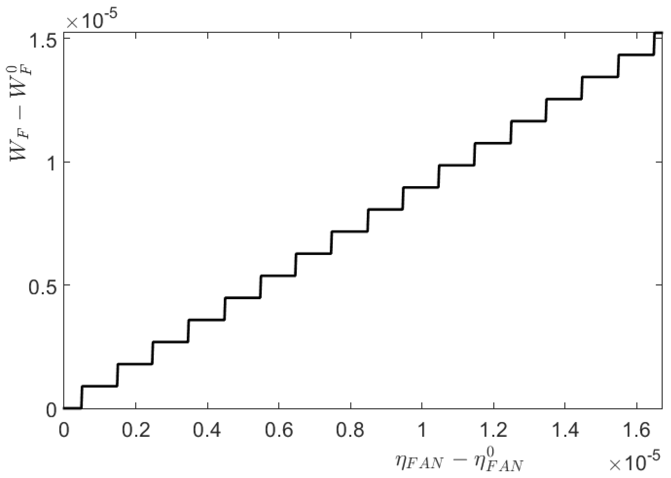
where, for $m=1,\dots ,N_{degrads}$, ${\mathbf{I}}_m$ is the m-th column of the $N_{degrads}\times N_{degrads}$ unit matrix. Note that this computation requires running the engine model $N_{degrads}+1$ times. In this approximation, the finite differences increment, $\delta >0$, is taken conveniently small, but not too small to avoid artifacts due to roundoff errors in the engine model solver, which is PROOSIS in the present application; similar roundoff artifacts are present in all engine models. The artifacts are illustrated in Figure 4, where the outcomes provided by PROOSIS for one of the outputs, $W_F$, are plotted vs. one of the inputs, ${\eta }_{FAN}$, in a representative input span. This plot shows a stairlike structure. Similar stairlike patterns are also observed when plotting other outputs vs. other inputs. If the finite differences increment, $\delta$, is too small, then the approximated derivative is equal to zero within each step and very large near the end-points of the steps. Such a spurious artifact can be eliminated by taking $\delta$ somewhat larger than the steps width, but still small to avoid losing accuracy in the derivatives computation. After some calibration (performed just once at the outset), considering the counterparts of Figure 4 for other scaled input–output pairs, it is observed that a good choice of the finite differences increment in the present application is $\delta$∼${10}^{-4}$. Once selected, this value of $\delta$ will be used in all diagnosis computations.

On the other hand, if the temperature $T_{4t}$ needs to be computed along with the $N_{degrads}$ degradations in the diagnosis process, then $T_{4t}$ is considered as a new 0-th unknown, $x_0$, and scaled such $x_0$ becomes $O\left(1\right)$. This is done here by defining

$$x_0=(T_{4t}-1300)/1300,$$

(12)

where the reference value 1300 is taken below typical cruise conditions (∼1400 K). The counterpart of the Jacobian computed above is a $N_{sensors}\times (1+N_{degrads})$-matrix

$${\mathbf{J}}_{T_{4t},\mathbf{x}}(T_{4t},\mathbf{x})=[{\mathbf{j}}_0,{\mathbf{j}}_1,\dots ,{\mathbf{j}}_{N_{degrads}}],$$

(13)

with the new 0-th column approximated as

$${\mathbf{j}}_0\simeq [\mathbf{F}(1300·(1+x_0+\delta ),\mathbf{x})-\mathbf{F}(1300·(1+x_0),\mathbf{x})]/\left(1300\delta \right),$$

(14)

while the remaining columns are computed as the counterparts of (11), namely

$${\mathbf{j}}_m\simeq [\mathbf{F}(1300·(1+x_0),\mathbf{x}+\delta {\mathbf{I}}_m)-\mathbf{F}(1300·(1+x_0),\mathbf{x})]/\delta ,$$

(15)

for $m=1,\dots ,N_{degrads}$.

Concentrating on the Jacobians (10), their condition number is a good means to anticipate how well gradient-like methods perform. In other words, the good functioning of these methods requires that the condition number be not too large. Unfortunately, using the default sensors set, this condition number is extremely large, since it varies from ${10}^5$ to ${10}^8$, depending on the value of the temperature $T_{4t}$ at which the Jacobian is computed. Moreover, the Hessian of the objective function associated with the optimization problem (8) is even much more ill-conditioned, since its condition number scales with the square of the condition number of the corresponding Jacobian. This means that solving the optimization problem (8) via a gradient-like method would be extremely problematic [35,36].

In order to obtain better conditioned gradient-like methods to solve the inverse problem, computations will be made collecting the sensor outcomes at two values of $T_{4t}$, called $T_{4t}^1$ and $T_{4t}^2$. Denoting the associated Jacobians as ${\mathbf{J}}_1$ and ${\mathbf{J}}_2$, we consider the enlarged Jacobian, of size $\left(2N_{sensors}\right)\times N_{degrads}$, defined as

$${\mathbf{J}}^{\mathrm{enlarged}}=\left[\begin{array}{c}{\mathbf{J}}_1\\ {\mathbf{J}}_2\end{array}\right].$$

(16)

This matrix is much better conditioned than the individual Jacobians. For instance, setting

$$T_{4t}^1=1350\mathrm{and}{T}_{4t}^2=1500,$$

(17)

which are below and above the typical value of $T_{4t}$∼1400 at cruise conditions, the condition number of ${\mathbf{J}}^{\mathrm{enlarged}}$ decreases to much smaller values, ∼350. Additional tests for other pairs of values of $T_{4t}^1$ and $T_{4t}^2$ provide very similar results, provided that $T_{4t}^1$ and $T_{4t}^2$ are not too close to each other. Increasing the number of the considered values of $T_{4t}$ (namely, taking three or more values), instead, does not decrease significantly the condition number of the enlarged Jacobian. Thus, using more than two values of $T_{4t}$ does not improve accuracy and robustness, while it penalizes the computational cost. In the remainder of this section, just two values of $T_{4t}$ will be used.

4.3. Computations Using an Optimization Method

In this method, for two sets of sensors outcomes, ${\mathbf{y}}_1^{\mathrm{measur}.}$ and ${\mathbf{y}}_2^{\mathrm{measur}.}$, obtained at the $T_{4t}$ temperature values $T_{4t}^1$ and $T_{4t}^2$, respectively, the following optimization problem is considered (cf. Equation (8))

$$\min \sqrt{{∥\mathbf{F}(T_{4t}^1,\mathbf{x})-{\mathbf{y}}_1^{\mathrm{measur}.}∥}_2^2+{∥\mathbf{F}(T_{4t}^2,\mathbf{x})-{\mathbf{y}}_2^{\mathrm{measur}.}∥}_2^2}.$$

(18)

Here, as in (8), ${\parallel ·\parallel }_2$ is the usual Euclidean norm and $\mathbf{F}(T_{4t}^1,\mathbf{x})$ and $\mathbf{F}(T_{4t}^2,\mathbf{x})$ are the associated (scaled) outcomes of the engine model, as defined in (7). This optimization problem is solved via the method implemented in the MATLAB function ‘sequential quadratic programming’ (SQP) [41]. The gradient of the objective function (18) will be computed by the SQP solver (by finite differences), using the option ‘Derivatives: approximated by the solver’; the Hessian is dynamically approximated by the solver via a BFGS Broiden method [35,36]. However, roundoff errors in the PROOSIS solver that is needed in the objective function computation, introduce spurious local minima. These local minima are eliminated by selecting the ‘minimum perturbation’ (whose default value is zero) to apply finite differences. The minimum perturbation is set as $5.5·{10}^{-4}$. This value has been selected after a slight calibration, attending to the robustness of the results, and will be maintained in all applications below. Concerning the type of finite differences to approximate derivatives, it is selected as forward differences.

An initial condition must be provided to initiate the SQP iterative process, as well as (a) constraints that, in the present case, impose that all degradations be non-negative and not larger than 2 (i.e., 2% with the scaling performed above); and (b) two tolerances, $TolFun-Data$ and $TolX-Data$, which control the stopping conditions by monitoring local increments in the objective function and the degradations, respectively. In the applications below, we shall set $TolFun-Data=TolX-Data={10}^{-4}$. In order to emphasize robustness, the initial condition will be randomly chosen (using, hereinafter, the MATLAB command ‘rand’) in the interval between 0 and 2 in each run.

Now, as anticipated, we consider two cases, one in which the values $T_{4t}^1$ and $T_{4t}^2$ of the temperature $T_{4t}$ are known (to compare with the previous approached in the literature) and another in which $T_{4t}^1$ and $T_{4t}^2$ are calculated along with the degradations.

The case in which the temperatures $T_{4t}^1$ and $T_{4t}^2$ are known is addressed in

Table 3. The optimization method applied to two representative cases, considered in columns 2–4 and 5–7. In both cases, the error in the degradation parameters is given in the second and fifth columns. Since these errors are fairly small in both cases, only the initial condition and the exact degradations are displayed.

x	${\mathbf{Error}}^x$	${\mathbf{x}}^{\mathbf{initial}}$	${\mathbf{x}}^{\mathbf{exact}}$	${\mathbf{Error}}^{\mathbf{x}}$	${\mathbf{x}}^{\mathbf{initial}}$	${\mathbf{x}}^{\mathbf{exact}}$
x(1)	$4.5·{10}^{-3}$	0.6551	1.0508	$9.8·{10}^{-3}$	1.0554	0.2234
x(2)	$1.3·{10}^{-2}$	1.3425	1.0607	$1.1·{10}^{-2}$	0.9591	0.2726
x(3)	$1.1·{10}^{-2}$	0.8773	1.7223	$6.7·{10}^{-3}$	1.6027	1.3573
x(4)	$2.0·{10}^{-2}$	1.6770	0.9697	$5.8·{10}^{-3}$	0.4557	0.9904
x(5)	$1.3·{10}^{-2}$	1.5377	0.7869	$3.3·{10}^{-3}$	0.9962	0.3794
x(6)	$1.5·{10}^{-2}$	0.3345	1.3429	$2.7·{10}^{-3}$	1.8017	0.9900
x(7)	$4.6·{10}^{-1}$	1.7240	1.4825	$1.2·{10}^{-1}$	1.1493	0.2952
x(8)	$2.7·{10}^{-2}$	1.9797	1.0401	$5.9·{10}^{-3}$	1.6904	0.1099
x(9)	$2.7·{10}^{-1}$	1.0288	0.6954	$7.4·{10}^{-2}$	1.4773	1.7014
x(10)	$6.5·{10}^{-1}$	1.7686	0.3000	$1.7·{10}^{-1}$	1.1720	1.1211

, for two representative outcomes of the method, using the values of $T_{4t}^1$ and $T_{4t}^2$ given in Equation (17), and considering two sets of (randomly chosen) degradations between 0 and 2. Note that, in both runs of the method, the errors for the 7-th, 9-th, and 10-th degradations are significantly larger (roughly, one order of magnitude larger) than for the remaining degradations. Moreover, it is remarkable that the method converges (to approximations of the exact degradations values) in spite of the fact that the randomly chosen initial conditions are not close at all to the ‘exact’ degradations. This suggests that the objective function exhibits a unique local minimum, as anticipated. The computational cost of each run of the method is ∼1.5 CPU minutes, performing ∼35 iterations. This is consistent with the computational cost of PROOSIS, which is ∼0.07 CPU seconds, since, at each iteration, the SQP MATLAB function requires 22 objective function evaluations to compute the gradient of the objective function by finite differences. The large number of iterations is due to the fact that the Hessian of the objective function is fairly ill-conditioned, as anticipated.

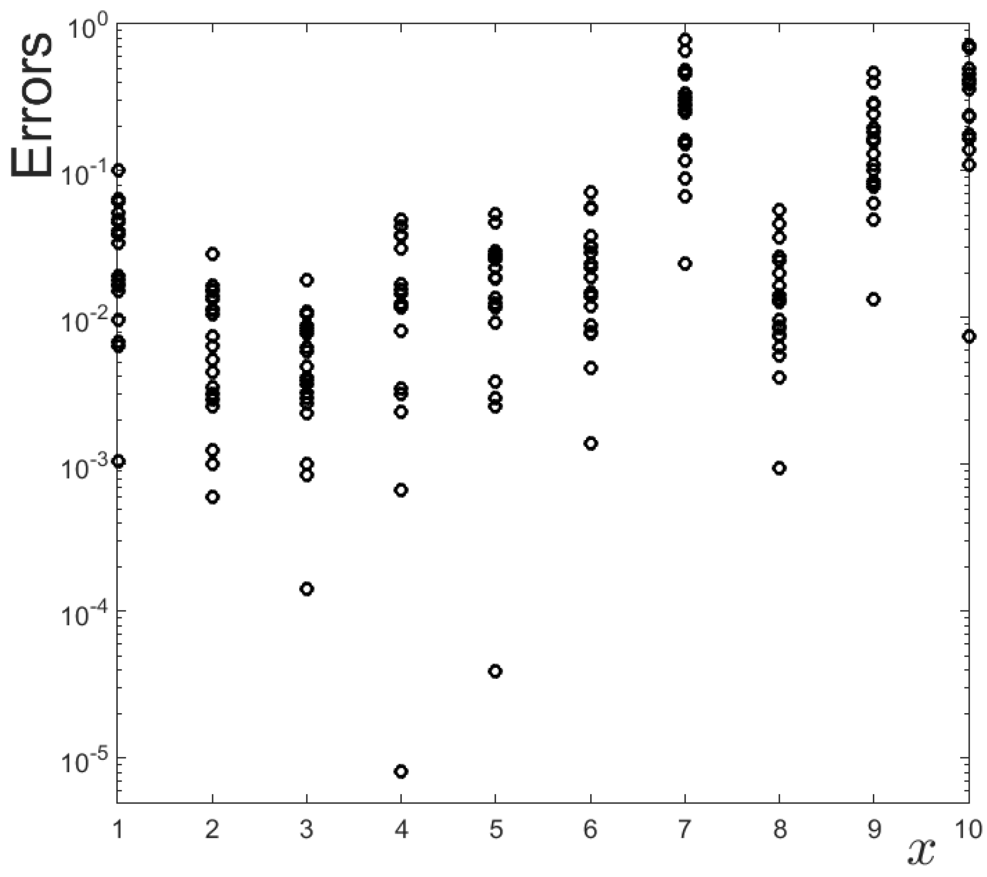
In order to evaluate the robustness of the method, the computations above have been repeated 20 times, always selecting the exact degradations randomly, and setting the initial conditions randomly as well. The obtained results are quite similar to those displayed in Table 3. In particular, the method always converges to the exact solution, and the accuracy is clearly worse for the 7-th, 9-th, and 10-th degradations than for the remaining degradations. The worse accuracy in these three degradations is illustrated in Figure 5.

Let us now turn to the second case, in which the values $T_{4t}^1$ and $T_{4t}^2$ of $T_{4t}$ must be computed along with the degradations. $T_{4t}^1$ and $T_{4t}^2$ are imposed to be in intervals of length equal to 100, around their unknown ‘exact’ values. As anticipated, the uncertainty of 50 (K) is consistent with the typical accuracy of the engine instrumentation. For convenience, the unknowns $T_{4t}^1$ and $T_{4t}^2$ are constrained to be in the disjoint intervals

$$T_{4t}^{1,\min }=1300\le T_{4t}^1\le T_{4t}^{1,\max }=1400,T_{4t}^{2,\min }=1450\le T_{4t}^2\le T_{4t}^{2,\max }=1550,$$

(19)

and rescaled as

$$x_0\left(j\right)=2\frac{T_{4t}^j-T_{4t}^{\mathrm{j},\min }}{T_{4t}^{\mathrm{j},\max }-T_{4t}^{\mathrm{j},\min }}\mathrm{for}j=1,2.$$

(20)

These are selected such that the intervals (19) are transformed into $0\le x_0\left(j\right)\le 2$, which coincide with the intervals in which the various degradations are allowed to vary in this section. Note that, once $x_0\left(1\right)$ and $x_0\left(2\right)$ are calculated, the unscaled values of $T_{4t}^1$ and $T_{4t}^2$ are recovered by solving (20) for $T_{4t}^j$.

Concerning the application of the SQP solver in this second case, the objective function is again given by (18), except that the number of scalar unknowns is now $N_{degrads}+2=12$ because $T_{4t}^1$ and $T_{4t}^2$ need to be computed by the solver. To emphasize robustness, the tunable parameters of the method are taken as identical to those used in the former case in which $T_{4t}^1$ and $T_{4t}^2$ were known. The method is somewhat slower in the present case, since each run requires ∼2 CPU minutes. This was to be expected since two additional unknowns are computed now, while the tunable parameters of the method are maintained. Two representative outcomes of the method are given in

Table 4. Counterpart of Table 3 for the case in which the temperatures $T_{4t}^1$ and $T_{4t}^2$ are computed along with the degradations. The (randomly selected) values of the exact temperatures are $(T_{4t}^1,T_{4t}^2)=(1345.5,1537.1)$ and $(T_{4t}^1,T_{4t}^2)=(1381.4,1474.4)$ for the cases considered in columns 2–4 and 5–7, respectively, and are all computed by the solver up to an error smaller than 1 (K).

x	${\mathbf{Error}}^{\mathbf{x}}$	${\mathbf{x}}^{\mathbf{initial}}$	${\mathbf{x}}^{\mathbf{exact}}$	${\mathbf{Error}}^{\mathbf{x}}$	${\mathbf{x}}^{\mathbf{initial}}$	${\mathbf{x}}^{\mathbf{exact}}$
x(1)	$8.5·{10}^{-2}$	1.1898	0.6222	$7.4·{10}^{-2}$	0.3313	1.0119
x(2)	$3.8·{10}^{-3}$	0.5244	1.8468	$3.9·{10}^{-3}$	1.2040	1.3982
x(3)	$2.7·{10}^{-2}$	1.2057	0.8604	$9.9·{10}^{-3}$	0.5259	1.7818
x(4)	$2.3·{10}^{-2}$	1.4224	0.3696	$1.4·{10}^{-2}$	1.3082	1.9186
x(5)	$5.5·{10}^{-2}$	0.4435	1.8098	$2.7·{10}^{-2}$	1.3784	1.0944
x(6)	$1.1·{10}^{-2}$	0.2348	1.9595	$8.6·{10}^{-4}$	1.4963	0.2773
x(7)	$2.7·{10}^{-1}$	0.5934	0.8777	$5.1·{10}^{-1}$	0.9011	0.2986
x(8)	$4.5·{10}^{-3}$	0.6376	0.2222	$8.3·{10}^{-3}$	0.1676	0.5150
x(9)	$1.9·{10}^{-1}$	0.8483	0.5161	$3.3·{10}^{-1}$	0.4580	1.6814
x(10)	$4.1·{10}^{-1}$	1.0157	0.8174	$7.5·{10}^{-1}$	1.8260	0.5086

.

Comparison of these results with those in Table 3 shows that, as in the former case, the 7-th, 9-th, and 10-th degradations are computed with much worse accuracy than the remaining degradations. Moreover the method converges well to the exact solution in spite of the fact that the initial condition is generally far from the correct solution, suggesting again that the optimization problem exhibits a unique local minimum.

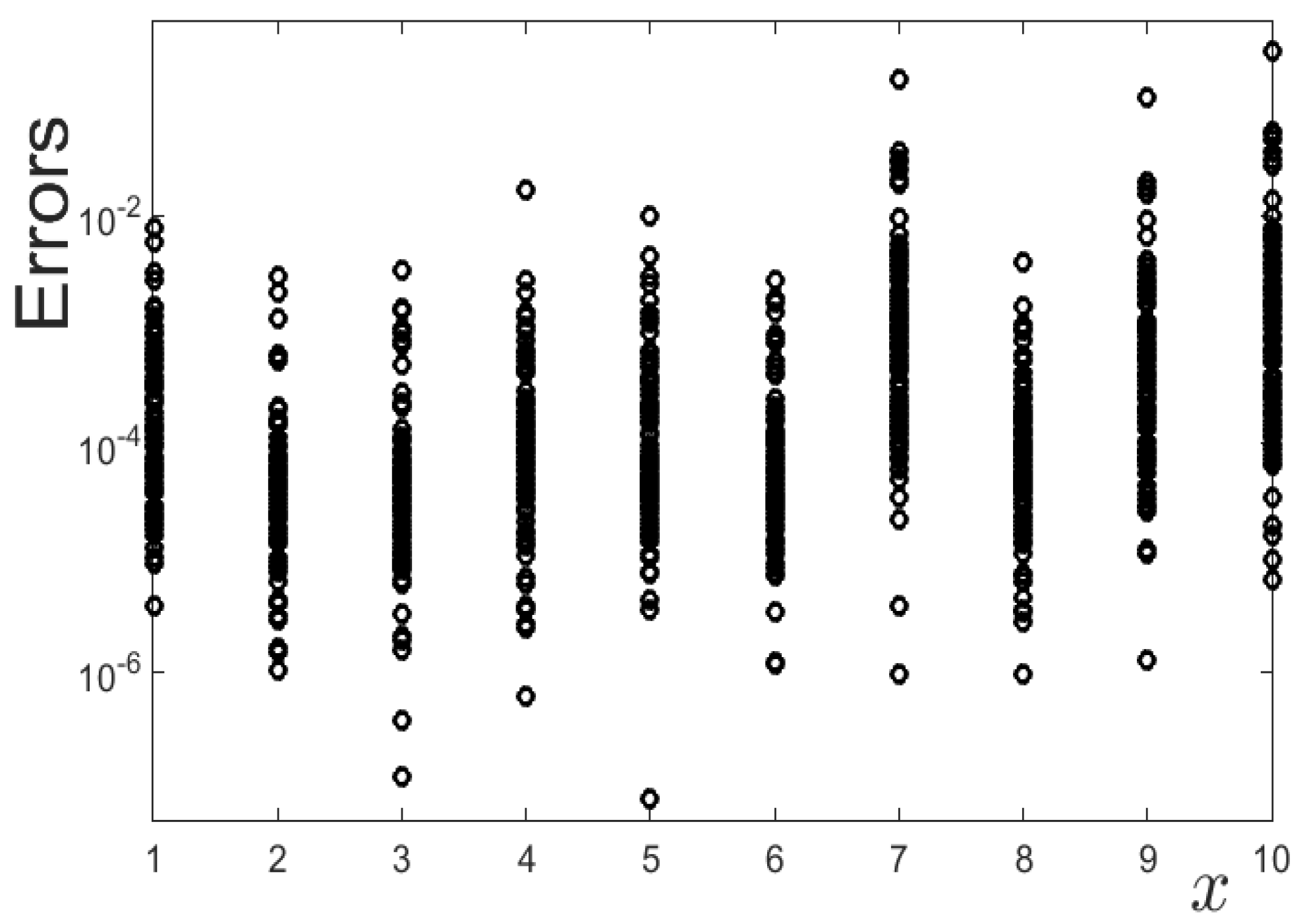
As in the former case, the robustness of the method has been tested by performing computations 20 times, always selecting the exact values of $T_{4t}^1$ and $T_{4t}^2$ and the degradations randomly, and setting the initial conditions randomly as well. The obtained errors are displayed in Figure 6, which shows that, again, the accuracy on the 7-th, 9-th, and 10-th degradations is generally much worse than for the remaining degradations. Moreover, results are quite similar to those displayed in Table 4. In particular, the method converges always to the exact solution (both the ten degradations and the two values of $T_{4t}$), suggesting once more that the solution to the diagnosis problem is unique.

4.4. Adapted Newton Method

Let us construct an adapted Newton method that allows for imposing constraints and discarding non-acceptable outcomes of the engine model. This iterative method is designed to solve the system of equations

$$\left[\begin{array}{c}\mathbf{F}(T_{4t}^1,\mathbf{x})\\ \mathbf{F}(T_{4t}^2,\mathbf{x})\end{array}\right]=\left[\begin{array}{c}{\mathbf{y}}_1^{\mathrm{measur}.}\\ {\mathbf{y}}_2^{\mathrm{measur}.}\end{array}\right]\equiv {\mathbf{y}}^{\mathrm{measur}.\text{-}\mathrm{enlarged}},$$

(21)

where $\mathbf{F}(T_{4t}^1,\mathbf{x})$, $\mathbf{F}(T_{4t}^2,\mathbf{x})$, ${\mathbf{y}}_1^{\mathrm{measur}.}$, and ${\mathbf{y}}_2^{\mathrm{measur}.}$ coincide with their counterparts in the optimization-based method, appearing in Equation (18).

The method needs an acceptable engine model initial condition, namely such that it is in the above mentioned acceptable region, where PROOSIS simulates the engine performance well. Such an initial condition is randomly chosen. As in standard Newton methods, subsequent iterations are calculated as follows. At the k-th iteration step, the new value of $\mathbf{x}$, ${\mathbf{x}}_{k+1}$, is computed as

$${\mathbf{x}}_{k+1}={\mathbf{x}}_k+\Delta {\mathbf{x}}_k,$$

(22)

where $\Delta {\mathbf{x}}_k$ is given by the following linear system

$${\mathbf{J}}_k^{\mathrm{enlarged}}\Delta {\mathbf{x}}_k={\mathbf{y}}^{\mathrm{measur}.\text{-}\mathrm{enlarged}}-{\mathbf{y}}_k^{\mathrm{enlarged}}.$$

(23)

Here, the enlarged Jacobian ${\mathbf{J}}_k^{\mathrm{enlarged}}$ is as defined in (16) and

$${\mathbf{y}}_k^{\mathrm{enlarged}}=\left[\begin{array}{c}\mathbf{F}(T_{4t}^1,{\mathbf{x}}_k)\\ \mathbf{F}(T_{4t}^2,{\mathbf{x}}_k)\end{array}\right].$$

(24)

At each iteration step, the over-determined linear system (23) is solved via the pseudo-inverse, whose computation is summarized here for the sake of clarity. To begin with, plain SVD (no truncation) is applied to ${\mathbf{J}}_k^{\mathrm{enlarged}}$, which gives

$${\mathbf{J}}_k^{\mathrm{enlarged}}={\mathbf{U}}_k{\mathbf{S}}_k{\mathbf{V}}_k^{\top }.$$

(25)

Then, $\Delta {\mathbf{x}}_k$ is computed as

$$\Delta {\mathbf{x}}_k={\mathbf{V}}_k{\mathbf{S}}_k^{-1}{\mathbf{U}}_k^{\top }\left[{\mathbf{y}}^{\mathrm{measur}.\text{-}\mathrm{enlarged}}-{\mathbf{y}}_k^{\mathrm{enlarged}}\right].$$

(26)

Now, using (22), it may happen that, at some step (specially, at the first steps), the new degradation vector, ${\mathbf{x}}_{k+1}$, is such that some of its components are negative, namely, they do not satisfy constraints. In this case, the negative degradations are set to zero and (22) is applied using the new values of ${\mathbf{x}}_k$. Likewise, it could happen that ${\mathbf{x}}_{k+1}$ becomes a non-acceptable engine model outcome. In this case (which has never occurred in our test runs but, in principle, could happen), the iterative process is discarded, a new (randomly chosen and acceptable) initial condition is selected, and a new iterative run is performed. We emphasize that, as described above, both the initial condition and the subsequent iterations are all acceptable engine model outcomes.

The resulting iterative method is much faster than the optimization-based method considered above, since it usually converges in less than 10 iteration steps. This is in spite of the fact that, consistently with the global character of the present method, initial conditions are taken randomly and of order one. The method is considered as converged if the following conditions hold

$$\parallel {\mathbf{x}}_{k+1}-{\mathbf{x}}_k{\parallel }_{\mathrm{RMS}}<{\epsilon }_1\mathrm{and}{∥{\mathbf{y}}^{\mathrm{measur}.\text{-}\mathrm{enlarged}}-{\mathbf{y}}_k^{\mathrm{enlarged}}∥}_{\mathrm{RMS}}<{\epsilon }_2,$$

(27)

for some small thresholds ${\epsilon }_1>0$ and ${\epsilon }_2>0$. Moreover, a maximum number of iteration steps is allowed. If, after these steps, conditions (27) are not met, the present iterative process is discarded, a new (acceptable) initial condition is randomly selected, and the iterative process is started again. This situation occurs in very few cases, since the process usually converges in less than 10 iteration steps. Moreover, the method converges always to the right solution, suggesting once again that the solution to the diagnosis problem is unique.

Representative outcomes of the present method are given in

Table 5. Counterpart of Table 3 using the adapted Newton method.

x	${\mathbf{Error}}^{\mathbf{x}}$	${\mathbf{x}}_0$	${\mathbf{x}}^{\mathbf{exact}}$	${\mathbf{Error}}^{\mathbf{x}}$	${\mathbf{x}}_0$	${\mathbf{x}}^{\mathbf{exact}}$
x(1)	$4.6·{10}^{-5}$	0.3658	0.0611	$7.9·{10}^{-5}$	0.6029	1.9033
x(2)	$4.9·{10}^{-5}$	0.4799	1.4881	$4.3·{10}^{-6}$	1.4022	1.8407
x(3)	$9.2·{10}^{-6}$	1.7730	1.0000	$9.4·{10}^{-5}$	1.3327	0.1054
x(4)	$1.4·{10}^{-4}$	0.0573	0.9598	$4.8·{10}^{-5}$	1.0783	1.4757
x(5)	$7.4·{10}^{-5}$	0.9798	1.8094	$5.0·{10}^{-5}$	1.3962	0.5382
x(6)	$7.1·{10}^{-5}$	0.3359	1.2197	$2.6·{10}^{-5}$	1.3331	0.8457
x(7)	$2.3·{10}^{-3}$	1.9574	1.2353	$1.8·{10}^{-3}$	0.3563	1.0957
x(8)	$2.7·{10}^{-5}$	1.4254	1.7189	$1.7·{10}^{-5}$	0.2560	1.8855
x(9)	$1.3·{10}^{-3}$	1.0009	1.6110	$1.2·{10}^{-3}$	1.9982	0.8355
x(10)	$3.5·{10}^{-3}$	0.9422	1.1534	$2.7·{10}^{-3}$	0.3422	1.9661

, as obtained when setting ${\epsilon }_1={10}^{-2}$, ${\epsilon }_2={10}^{-3}$, and allowing 15 iteration steps.

Note that we have taken the thresholds ${\epsilon }_1$ and ${\epsilon }_2$ to be very small, which has given small errors in the degradations. This has been done on purpose, to illustrate the very good convergence of the method, which is due to the fact that the condition number of the Jacobian, ∼300, is much smaller than its counterpart for the Hessian appearing in the former subsection, which was ∼${10}^5$. Table 5 also shows that, as it happened with the optimization-based method considered in Section 4.3, the errors for the 7-th, 9-th, and 10-th degradations are clearly larger than for the remaining degradations. The computational cost of each run is ∼10 CPU seconds (thus, much smaller than the cost of the optimization-based method) to obtain results that are much more accurate, as the comparison with Table 3 shows.

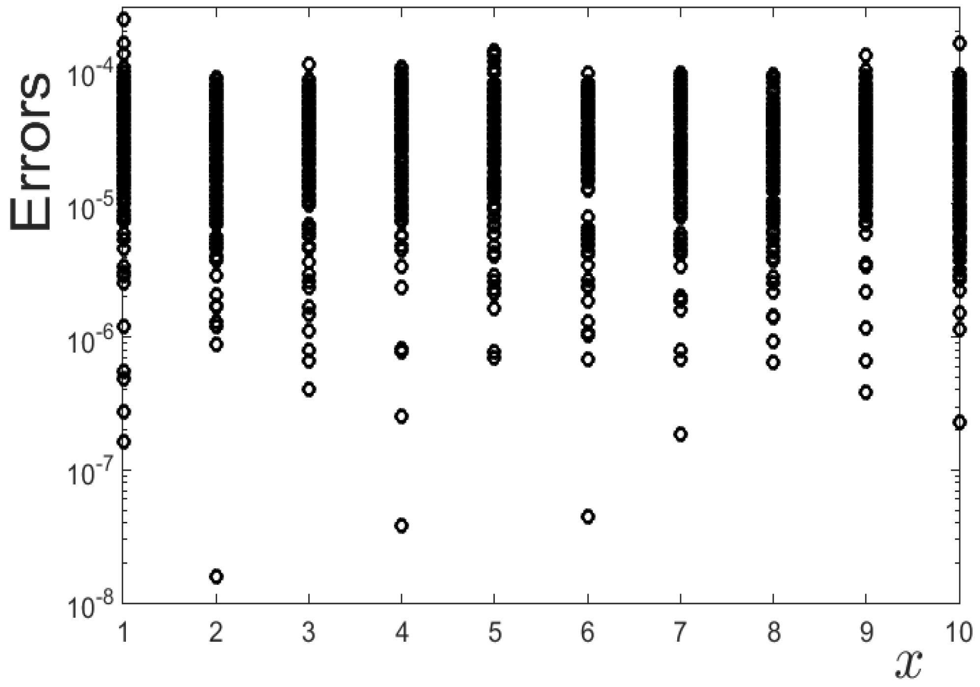
As we did for the optimization-based method, in order to further ensure the robustness, the computations above have been repeated 100 times, always selecting the exact degradations randomly and setting random initial conditions as well. The obtained results are consistent with those displayed in Table 5. In particular, for any initial condition, the method converges to the right solution, confirming once more that the inverse problem exhibits a unique solution. Moreover, the accuracy is clearly worse for the 7-th, 9-th, and 10-th degradations than for the remaining ones, as illustrated in Figure 7.

4.5. Correlations between Degradations and Consequences

In the obtained diagnosis results using various methods, the 7-th, 9-th, and 10-th degradations were systematically computed with less accuracy than the remaining degradations; see Table 3, Table 4 and Table 5, and Figure 5, Figure 6 and Figure 7. Obviously, there must be a reason for this fact, which is analyzed now by seeking correlations between degradations.

The analysis is based on the Jacobians ${\mathbf{J}}_{\mathbf{x}}(T_{4t},\mathbf{x})$ (as defined in (10)), which in the present case are $10\times 10$-matrices. For instance, considering these Jacobians at zero-degradations (undegraded state), ${\mathbf{J}}_{\mathbf{x}}(T_{4t},\mathbf{0})$, for various representative values of $T_{4t}$, their condition number is larger than ∼${10}^5$.

A deeper insight is gained considering the singular values of these matrices, displayed in Table 6, where it can be observed that the singular values are comparable among each other for the five considered values of $T_{4t}$. Moreover, the 10-th singular value is always three orders of magnitude smaller than the remaining ones, which can be taken advantage of to obtain approximate correlations among degradations, as explained in Section 2. Since degradations correspond to the columns of the Jacobian, the relevant correlations are as displayed in Equation (5), which provides as many approximate correlations as the number of singular values that are much smaller than the remaining ones. In the present case, only the last singular value satisfies this property, which means that only one approximate correlation is obtained. Such an approximate correlation between the elements of each Jacobian ${\mathbf{J}}_{\mathbf{x}}(T_{4t},\mathbf{0})$, denoted here as

$${\mathbf{J}}_{\mathbf{x}}(T_{4t},\mathbf{0})=\mathbf{A},$$

(28)

is the counterpart of (5), which can be written as

$$\sum _{j=1}^{10}{a}_j{A}_{ij}\simeq 0,\mathrm{with}{a}_j=V_{j10},$$

(29)

where, for $j=1,\dots ,10$, $V_{j10}$ are the elements of the last column of the right SVD mode (associated with the very small singular value) defined in (1). The approximate correlations (29) can be considered as approximate correlations between the ten degradations, namely

$$\sum _{j=1}^{10}{a}_{j}x\left(j\right)\simeq 0.$$

(30)

The coefficients $a_1,a_2,\dots ,a_{10}$ for the five values of $T_{4t}$ considered in Table 6 are given in

Table 7. The coefficients appearing in (30) for the values of $T_{4t}$ already considered in Table 6.

${\mathit{T}}_{4\mathit{t}}$	$100{\mathit{a}}_1$	$100{\mathit{a}}_2$	$100{\mathit{a}}_3$	$100{\mathit{a}}_4$	$100{\mathit{a}}_5$	$100{\mathit{a}}_6$	${\mathit{a}}_7$	$100{\mathit{a}}_8$	${\mathit{a}}_9$	${\mathit{a}}_{10}$
1300	−0.003	0.001	0.03	0.06	0.15	0.13	−0.53	−0.06	0.31	−0.79
1350	0.000	−0.005	−0.04	−0.07	−0.12	−0.05	0.53	0.05	−0.31	0.79
1400	0.009	0.002	0.05	0.06	0.06	0.02	−0.53	−0.04	0.32	−0.79
1450	0.005	0.003	0.02	0.06	0.07	0.03	−0.53	−0.03	0.32	−0.79
1500	0.011	0.001	0.06	0.10	0.01	0.01	−0.53	−0.03	0.32	−0.79

.

Table 6. Singular values of the Jacobians of the sensors with respect to the degradations at zero degradations, ${\mathbf{J}}_{\mathbf{x}}(T_{4t},\mathbf{0})$, for the indicated values of $T_{4t}$.

${\mathit{T}}_{4\mathit{t}}$	${\mathit{s}}_1$	${\mathit{s}}_2$	${\mathit{s}}_3$	${\mathit{s}}_4$	${\mathit{s}}_5$	${\mathit{s}}_6$	${\mathit{s}}_7$	${\mathit{s}}_8$	${\mathit{s}}_9$	${\mathit{s}}_{10}$
1300	$0.629$	$0.498$	$0.113$	$0.099$	$0.071$	$0.047$	$0.040$	$0.022$	$0.013$	$4.4·{10}^{-7}$
1350	$0.772$	$0.429$	$0.114$	$0.104$	$0.078$	$0.055$	$0.042$	$0.023$	$0.014$	$3.2·{10}^{-6}$
1400	0.851	$0.409$	$0.115$	$0.107$	$0.085$	$0.060$	$0.044$	$0.024$	$0.015$	$4.5·{10}^{-6}$
1450	0.884	$0.382$	$0.118$	$0.111$	$0.093$	$0.065$	$0.046$	$0.025$	$0.016$	$6.1·{10}^{-6}$
1500	0.903	$0.382$	$0.124$	$0.117$	$0.099$	$0.070$	$0.048$	$0.027$	$0.016$	$1.1·{10}^{-5}$

Table 6. Singular values of the Jacobians of the sensors with respect to the degradations at zero degradations, ${\mathbf{J}}_{\mathbf{x}}(T_{4t},\mathbf{0})$, for the indicated values of $T_{4t}$.

${\mathit{T}}_{4\mathit{t}}$	${\mathit{s}}_1$	${\mathit{s}}_2$	${\mathit{s}}_3$	${\mathit{s}}_4$	${\mathit{s}}_5$	${\mathit{s}}_6$	${\mathit{s}}_7$	${\mathit{s}}_8$	${\mathit{s}}_9$	${\mathit{s}}_{10}$
1300	$0.629$	$0.498$	$0.113$	$0.099$	$0.071$	$0.047$	$0.040$	$0.022$	$0.013$	$4.4·{10}^{-7}$
1350	$0.772$	$0.429$	$0.114$	$0.104$	$0.078$	$0.055$	$0.042$	$0.023$	$0.014$	$3.2·{10}^{-6}$
1400	0.851	$0.409$	$0.115$	$0.107$	$0.085$	$0.060$	$0.044$	$0.024$	$0.015$	$4.5·{10}^{-6}$
1450	0.884	$0.382$	$0.118$	$0.111$	$0.093$	$0.065$	$0.046$	$0.025$	$0.016$	$6.1·{10}^{-6}$
1500	0.903	$0.382$	$0.124$	$0.117$	$0.099$	$0.070$	$0.048$	$0.027$	$0.016$	$1.1·{10}^{-5}$

As can be observed, the dominant coefficients are $a_7$, $a_9$, and $a_{10}$, since the remaining coefficients are three orders of magnitude smaller. Moreover, the combination of these three dominant coefficients very approximately coincides for all values of $T_{4t}$, except for the (common) sign, which does not affect Equation (30). All these lead to an approximate correlation between the 7-th, 9-th, and 10-th degrations,

$$a_{7}x\left(7\right)+a_{9}x\left(9\right)+a_{10}x\left(10\right)\simeq 0,$$

(31)

which, in principle, could suggest ignoring one of these three degradations in the inverse problem computation; the ignored degradation would be obtained a posteriori using the correlation (31).

However, although the correlation (31) is consistent with the fact that the computation of these degradations was systematically worse than for the remaining degradations using different methods, the use of this correlation to eliminate one of the degradations would be misleading. In fact, based on physical grounds, we anticipate that this correlation is spurious, and just due to a non-optimal (from a diagnosis point of view) choice of the sensors. In fact, according to the nature of the 10 degradations, displayed in Table 1, the three problematic degradations are related to properties of the high and low pressure turbines, HPT and LPT, respectively. In particular, the (most problematic) 10-th degradation is related to the flow capacity of the LPT, which depends on the total pressure between the HTP and LTP, $P_{45t}$, that is not accounted for in the considered default set of sensors. It turns out that adding a new sensor measuring $P_{45t}$ is a good means to improve the former sensors’ set. Using this new sensors set, the Jacobian at zero degradations, ${\mathbf{J}}_{\mathbf{x}}(T_{4t},\mathbf{0})$, becomes a $11\times 10$-matrix, whose condition number for the same values of $T_{4t}$ considered above is ∼50, and is thus dramatically smaller than its counterpart using the former ten default sensors, which was always larger than ∼${10}^5$. In addition, similarly, the moderate condition numbers are obtained for the $11\times 11$ Jacobians (13) that also take dependence on $T_{4t}$ into account. These are very good news, suggesting that using the new improved set of sensors, will permit obtaining very good diagnosis results with data at just one value of $T_{4t}$, which is confirmed in the next section.

5. Diagnosis Using Data from the Improved Set of 11 Sensors

Now, we use data provided by the former 10 default sensors considered in the former section plus the new sensor giving $P_{45t}$ at just one value of $T_{4t}$, which will be computed along with the degradations. After the analysis in Section 4, we may guess that the adapted Newton method is better than the optimization-based method. Thus, it will be the adapted Newton method that will be used below to obtain both the degradations and $T_{4t}$. The optimization method provides good results too, but, as in the former section, its computational cost is larger and is not considered here.

As in Section 4, the same $N_{\mathrm{Degrad}.}=10$ degradations considered there are to be computed here, allowing them to vary in the range from 0 to 2 (%), although this range will be enlarged later on to illustrate the robustness of the method. Concerning the unknown value of $T_{4t}$, it is allowed to vary in the same range as in the former section, namely equal to $\pm 50$ K around the estimated value provided by the engine instrumentation.

The unknown value of $T_{4t}$ is scaled as (cf. Equation (20))

$$x_0=2\frac{T_{4t}-T_{4t}^{\min }}{T_{4t}^{\max }-T_{4t}^{\min }},$$

(32)

meaning that $x_0$ is constraint to the range $0\le x_0\le 2$. The sensor data are scaled as explained in Section 4.1, but applied to the new set of 11 sensors.

The adapted Newton method considered here is a straight forward extension of that developed in Section 4.4, except that now only one value of $T_{4t}$ is used, which is computed along with the degradations. In particular, as in Section 4.4, both the initial condition and all subsequent iterations are imposed to be acceptable engine model outcomes. Moreover, the adapted Newton method considered in Section 4.4 is modified as follows. Equation (21) is substituted by

$$\mathbf{F}(T_{4t},\mathbf{x})={\mathbf{y}}^{\mathrm{measur}.},$$

(33)

which involves the eleven unknowns formed by $T_{4t}$ and the ten components of the degradation vector $\mathbf{x}$. The function $\mathbf{y}=\mathbf{F}(T_{4t},\mathbf{x})$ represents the outcome of the direct problem (computed with PROOSIS) and ${\mathbf{y}}^{\mathrm{measur}.}$ collects the measured sensors vector, whose size is eleven. In fact, the unknown $T_{4t}$ is rescaled as indicated above in the application of the adapted Newton method, which substitutes (33) by

$$\mathbf{F}\left(\widehat{\mathbf{x}}\right)={\mathbf{y}}^{\mathrm{measur}.},$$

(34)

where the vector $\widehat{\mathbf{x}}$, whose size is 11, collects the 0-th degradation associated with $T_{4t}$ and the remaining 10 degradations included in the degradation vector $\mathbf{x}$. Then, beginning with an (acceptable) initial condition ${\widehat{\mathbf{x}}}_0$, the iterative method proceeds by computing, in the k-th iteration, the new value of $\widehat{\mathbf{x}}$ as

$${\widehat{\mathbf{x}}}_{k+1}={\widehat{\mathbf{x}}}_k+\Delta {\widehat{\mathbf{x}}}_k,$$

(35)

where $\Delta {\widehat{\mathbf{x}}}_k$ is computed by the linear system

$${\widehat{\mathbf{J}}}_k\Delta {\widehat{\mathbf{x}}}_k={\mathbf{y}}^{\mathrm{measur}.}-{\mathbf{y}}_k,$$

(36)

which is obtained upon linearization (34) around ${\widehat{\mathbf{x}}}_k$. Thus, ${\widehat{\mathbf{J}}}_k$ is the Jacobian of the left-hand side of (34) (which, as observed above, is reasonably well conditioned) at ${\widehat{\mathbf{x}}}_k$, ${\mathbf{y}}^{\mathrm{measur}.}$ is as given in the right-hand side of (34), and ${\mathbf{y}}_k=\mathbf{F}\left({\widehat{\mathbf{x}}}_k\right)$. To impose constraints in $\widehat{\mathbf{x}}$, if some of its components are smaller than zero, then these components (if any) are set to zero.

The iterative method proceeds until the following stopping conditions holds (cf. Equation (27))

$$\parallel {\widehat{\mathbf{x}}}_{k+1}-{\widehat{\mathbf{x}}}_k{\parallel }_{\mathrm{RMS}}<{\epsilon }_1,{\parallel {\mathbf{y}}^{\mathrm{measur}.}-{\mathbf{y}}_k\parallel }_{\mathrm{RMS}}<{\epsilon }_2.$$

(37)

Moreover, a maximum number of iteration steps is allowed and if, after this number of steps, conditions (37) do not hold, then the outcome is not accepted and the iterative process is repeated. This latter situation almost never occurs.

To begin with the illustration of the method, we consider two representative cases in which the exact values of the unknowns and the initial condition both satisfy the above mentioned constraints, with incremental degradations smaller than 2% and allowing $T_{4t}$ to vary in a range of $\pm 50$ K around its exact value. The thresholds (37) are taken as ${\epsilon }_1={\epsilon }_2={10}^{-4}$ in both cases, in which convergence (with these thresholds) is attained in ∼4 iteration steps, which require ∼5 CPU seconds.

The outcomes for these two cases are given in

Table 8. Counterpart of Table 5 but using the 11 sensors considered in this section (which include data for $P_{45t}$) allowing for 2 (%) degradations. The exact values of $T_{4t}$ are 1349.2 K and 1303.0 K for the cases considered in columns 2–4 and 5–7, respectively. These exact values are computed by the method with an error smaller than 0.1 (K).

x	${\mathbf{Error}}^{\mathbf{x}}$	${\mathbf{x}}_0$	${\mathbf{x}}^{\mathbf{exact}}$	${\mathbf{Error}}^{\mathbf{x}}$	${\mathbf{x}}_0$	${\mathbf{x}}^{\mathbf{exact}}$
x(1)	$5.8·{10}^{-5}$	0.7609	0.5022	$2.8·{10}^{-5}$	0.9011	0.6742
x(2)	$1.4·{10}^{-5}$	1.1356	1.2321	$2.4·{10}^{-5}$	0.1676	0.3244
x(3)	$3.5·{10}^{-5}$	0.1517	0.9466	$3.8·{10}^{-5}$	0.4580	1.5886
x(4)	$9.7·{10}^{-6}$	0.1079	0.7033	$4.1·{10}^{-5}$	1.8267	0.6224
x(5)	$5.1·{10}^{-5}$	1.0616	1.6617	$3.9·{10}^{-5}$	0.3048	1.0571
x(6)	$5.4·{10}^{-5}$	1.5583	1.1705	$2.4·{10}^{-7}$	1.6516	0.3313
x(7)	$4.9·{10}^{-5}$	1.8680	1.0994	$2.7·{10}^{-5}$	1.0767	1.2040
x(8)	$7.7·{10}^{-6}$	0.2598	1.8344	$8.3·{10}^{-6}$	1.9923	0.5259
x(9)	$2.0·{10}^{-5}$	1.1376	0.5717	$8.5·{10}^{-6}$	0.1564	1.3082
x(10)	$2.3·{10}^{-5}$	0.9388	1.5144	$5.3·{10}^{-5}$	0.8854	1.3784

, where it can be observed that, as anticipated, using the improved set of 11 sensors leads to very good results. This is in spite of the fact that just one value of $T_{4t}$ is needed, instead of the two values that were required when the former set of 10 sensors were used. Moreover, comparison of this table with Table 5 shows that the exact value of $T_{4t}$ is computed with great accuracy, as are the outcomes for the ten degradations. In addition, no spurious artifacts are appreciated in the outcomes for the 7-th, 9-th, and 10-th degradations; namely, the values of ${\mathrm{Error}}^{\mathbf{x}}$ for these three degradations and the remaining ones are comparable. This is illustrated in Figure 8, which (consistently with the results displayed in Table 8) shows the errors for outcomes when the method is applied 100 times, and it is always randomly selecting the exact outcomes and initial conditions. Thus, our guess in Section 4.5 that these spurious artifacts were just due to a deficient selection of the sensors is confirmed.

In summary, using the improved set of eleven sensors provides extremely good results. Moreover, these results are obtained considering just one value of $T_{4t}$, which was impossible using the default set of sensors.

Let us now check the performance of the method when noise is added to the sensors data, to somewhat mimic the noisy outcomes in actual sensors mounted in the engine. To this end, we add uniformly distributed random noise (computed with the MATLAB command ‘rand’) with a zero mean of size 0.005 (i.e., 0.5%) to the sensors data and apply the adapted Newton method. This level of noise represents the typical accuracy of the engine instrumentation. Although more sophisticated tools for noise filtering could be used, these are well beyond the scope of this paper, where a preliminary, simple, and natural error filtering tool is used. Specifically, the noise is filtered here by repeating computations 20 times (always with the same initial condition) and taking the means of the obtained values of $T_{4t}$ and the degradations. Results using this averaged, adapted Newton method are displayed in

Table 9. Counterpart of Table 8 when adding random noise to the sensors data. The temperature $T_{4t}$ is computed with an error ∼0.2 K.

x	${\mathbf{Error}}^{\mathbf{x}}$	${\mathbf{x}}_0$	${\mathbf{x}}^{\mathbf{exact}}$	${\mathbf{Error}}^{\mathbf{x}}$	${\mathbf{x}}_0$	${\mathbf{x}}^{\mathbf{exact}}$
x(1)	$1.6·{10}^{-1}$	0.7609	0.5022	$1.6·{10}^{-1}$	0.9011	0.6742
x(2)	$4.6·{10}^{-2}$	1.1356	1.2321	$5.1·{10}^{-2}$	0.1676	0.3244
x(3)	$3.9·{10}^{-2}$	0.1517	0.9466	$4.3·{10}^{-2}$	0.4580	1.5886
x(4)	$1.0·{10}^{-1}$	0.1079	0.7033	$8.4·{10}^{-2}$	1.8267	0.6224
x(5)	$1.0·{10}^{-1}$	1.0616	1.6617	$9.8·{10}^{-2}$	0.3048	1.0571
x(6)	$7.8·{10}^{-2}$	1.5583	1.1705	$1.1·{10}^{-1}$	1.6516	0.3313
x(7)	$4.4·{10}^{-2}$	1.8680	1.0994	$6.0·{10}^{-2}$	1.0767	1.2040
x(8)	$7.9·{10}^{-2}$	0.2598	1.8344	$8.4·{10}^{-2}$	1.9923	0.5259
x(9)	$5.5·{10}^{-2}$	1.1376	0.5717	$5.7·{10}^{-2}$	0.1564	1.3082
x(10)	$6.1·{10}^{-2}$	0.9388	1.5144	$9.2·{10}^{-2}$	0.8854	1.3784

for the same case considered in Table 8. In each of the 20 applications of the adapted Newton method, the thresholds appearing in (37) are taken to be larger than in the clean case, namely ${\epsilon }_1={\epsilon }_2={10}^{-2}$, and the adapted Newton method usually requires ∼4 iterations.

As can be observed in Table 9, the errors in the obtained degradations are reasonably small; namely, the accuracy is sufficient for the practical implementation of the tool, since it permits discerning safely which degradations remain small from those that require attention. In fact, the practical implementation of the tool would be performed by using a moving means on the turbine inlet temperature and the sensor outcomes during the engine operation. Taking into account that 4 iterations are needed in each of the 20 runs, the total computational time is ∼210 CPU seconds. This permits obtaining diagnosis results many times in each flight.

In summary, the adapted Newton method, considering just one value of $T_{4t}$, provides very good results even when random noise, of a realistic size, is added to the sensors data.

Given the success of the adapted Newton method in the former case, in which the degradations were allowed to be up to 2 (%), let us elucidate whether the performance of the method remains very good for larger degradations. In fact, in order to check the performance of the method, we allow for degradations as large as 30 (%). Such a level of maximum degradations is so large that it includes cases that would produce very dangerous events. However, such a degradation level can confirm the robustness of the methodology, which is able to accurately detect these very strong degradations as well. Results for this case are illustrated in

Table 10. Counterpart of Table 8 but allowing 30 (%) perturbations in the degradations. The exact values of $T_{4t}$ are 1391.6 K and 1490.9 K for the cases considered in columns 2–4 and 5–7, respectively, and are computed by the method with an error smaller than 0.1 K.

x	${\mathbf{Error}}^{\mathbf{x}}$	${\mathbf{x}}_0$	${\mathbf{x}}^{\mathbf{exact}}$	${\mathbf{Error}}^{\mathbf{x}}$	${\mathbf{x}}_0$	${\mathbf{x}}^{\mathbf{exact}}$
x(1)	$7.8·{10}^{-5}$	3.8185	3.0257	$9.0·{10}^{-5}$	28.196	20.042
x(2)	$2.3·{10}^{-5}$	0.4707	14.968	$2.3·{10}^{-5}$	25.013	14.436
x(3)	$2.5·{10}^{-5}$	22.593	7.1710	$5.8·{10}^{-5}$	4.6572	8.5849
x(4)	$6.4·{10}^{-5}$	15.145	10.488	$1.9·{10}^{-5}$	24.913	17.855
x(5)	$8.2·{10}^{-5}$	21.663	16.748	$1.9·{10}^{-5}$	13.924	10.092
x(6)	$1.0·{10}^{-5}$	22.833	16.442	$4.2·{10}^{-5}$	8.9207	28.786
x(7)	$4.9·{10}^{-5}$	8.0685	12.638	$1.3·{10}^{-5}$	15.699	13.262
x(8)	$8.5·{10}^{-6}$	5.8087	11.565	$2.7·{10}^{-5}$	24.949	28.860
x(9)	$3.3·{10}^{-6}$	1.9245	11.420	$8.4·{10}^{-6}$	16.174	20.292
x(10)	$8.1·{10}^{-5}$	12.761	8.4219	$5.8·{10}^{-5}$	7.7950	21.182

, where it can be observed that the obtained results are consistently good and comparable for all degradations, which means that the improved set of sensors is robust in connection with noise. Such robustness is further checked by repeating computations 100 times, always selecting randomly the exact outcomes and the initial conditions. The obtained errors in these 100 computations are illustrated in Figure 9, where it is observed that the errors in these cases are consistent with their counterparts in Table 10.

As in the former case, the effect of noise is analyzed by adding to the sensors data random noise of the same size as above and applying the already mentioned averaged and adapted Newton method. Results are displayed in

Table 11. Counterpart of Table 10 when adding random noise to the sensors’ data. The temperature $T_{4t}$ is computed with an error ∼0.2 K.

x	${\mathbf{Error}}^{\mathbf{x}}$	${\mathbf{x}}_0$	${\mathbf{x}}^{\mathbf{exact}}$	${\mathbf{Error}}^{\mathbf{x}}$	${\mathbf{x}}_0$	${\mathbf{x}}^{\mathbf{exact}}$
x(1)	$2.4·{10}^{-1}$	3.8185	3.0257	$1.8·{10}^{-1}$	28.196	20.042
x(2)	$2.0·{10}^{-2}$	0.4707	14.968	$3.4·{10}^{-2}$	25.013	14.436
x(3)	$5.9·{10}^{-2}$	22.593	7.1710	$4.5·{10}^{-2}$	4.6572	8.5849
x(4)	$8.4·{10}^{-2}$	15.145	10.488	$9.2·{10}^{-2}$	24.913	17.855
x(5)	$1.2·{10}^{-1}$	21.663	16.748	$1.6·{10}^{-1}$	13.924	10.092
x(6)	$1.2·{10}^{-1}$	22.833	16.442	$7.7·{10}^{-2}$	8.9207	28.786
x(7)	$6.5·{10}^{-2}$	8.0685	12.638	$9.2·{10}^{-2}$	15.699	13.262
x(8)	$1.3·{10}^{-1}$	5.8087	11.565	$1.7·{10}^{-1}$	24.949	28.860
x(9)	$6.8·{10}^{-2}$	1.9245	11.420	$1.0·{10}^{-1}$	16.174	20.292
x(10)	$8.6·{10}^{-2}$	12.761	8.4219	$1.6·{10}^{-1}$	7.7950	21.182

, where it can be observed, once more, that the method filters error reasonably well, in spite of the very large degradations. As in the previous case, the method permits discerning safely which degradations remain small from those that require attention, and the practical implementation can be made similarly, using moving means. As per the total computational time, the method usually requires ∼6 iterations per case and requires ∼250 CPU seconds, which is appropriate to perform this computation many times in each flight.

Summarizing the results in this section, the good choice of the sensors set selected in Section 4.5 has been confirmed. Moreover, using these sensors, the adapted Newton method was able to give very accurate and robust results, for both the unknown (up to 30%) degradations and the unknown value of $T_{4t}$. In addition, results are robust in connection with noise added to the data.

6. Concluding Remarks

A model-based methodology was developed for the efficient diagnosis of aeroengines, keeping in mind its potential industrialization. The methodology is transparent to both the specific aeroengine and the engine model, and was illustrated considering a representative aeroengine and a representative engine model. Several complementary tools were constructed that are able to:

• Compute the engine degradation (which can be very large) from a baseline state using data obtained in a set of sensors, as well as the value of the turbine inlet temperature, $T_{4t}$, at which these data have been acquired. As explained in the introduction, this represents a crucial advantage of the developed methodology.
• Evaluate a given set of sensors, obtaining clues to improve deficient sensor sets. By deficient sensor sets, we mean sets such that the Jacobian of the function providing the sensors data in terms of the degradations is quite ill-conditioned.

The calculation of the engine degradation and the associated values of $T_{4t}$ has been performed using two type of tools. The first type consisted in minimizing the RMS difference between the actual sensors data and their counterparts computed by the engine model. However, using the default set of sensors that is most frequently used in diagnosis studies, sensors data at two different values of $T_{4t}$ were needed because this default set of sensors is deficient. The obtained results exhibited a unique minimum, suggesting that the sensors data determine the engine degradation well (provided that data at two values of $T_{4t}$ are used). In addition, a second tool was developed that was based on an adapted Newton method that is able to take constraints into account and, also, to discard non-acceptable, unphysical engine model outcomes. This method is also robust, but much faster and much more precise than the former optimization-based method.

However, both the optimization-based and adapted Newton methods led to results that were systematically worse for some of the degradations. Such a property was analyzed with care, concluding that some spurious correlations among the obtained degradations were present, which is consistent with the fact that the default set of sensors is a deficient set. The analysis also suggested how this deficient set can be improved, by adding data in a convenient new sensor. Using the improved set of sensors, only data at one value of $T_{4t}$ was needed and, moreover, the adapted Newton method was much faster and yielded quite robust and much more precise results. In addition, these results were observed to be robust against random noise added to the data, which is very good news, keeping in mind the practical implementation of the methodology.

The small computational time required by the adapted Newton method using the improved set of sensors could be further reduced to approach a real time diagnosis, using a data-driven reduced order model. However, the development of this reduced order model is well beyond the scope of this paper and left as the object of future research.

References

1. Jardine, A.K.S.; Lin, D.; Banjevic, D. A review on machinery diagnostics and prognostics implementing condition-based maintenance. Mech. Syst. Signal Process. 2006, 20, 1483–1510. [Google Scholar] [CrossRef]
2. International Air Transport Association. Airline Maintenance Cost Executive Commentary (FY2018 Data). Available online: https://www.iata.org/ (accessed on 12 December 2021).
3. Li, Z.; Wang, Y.; Wang, K. Intelligent predictive maintenance for fault diagnosis and prognosis in machine centers: Industry 4.0 scenario. Adv. Manuf. 2017, 5, 377–387. [Google Scholar] [CrossRef]
4. Davari, N.; Veloso, B.; Costa, G.d.A.; Pereira, P.M.; Ribeiro, R.P.; Gama, J. A survey on data-driven predictive maintenance for the Railway industry. Sensors 2021, 21, 5739. [Google Scholar] [CrossRef] [PubMed]
5. Knotts, R.M.H. Civil aircraft maintenance and support fault diagnosis from a business perspective. SIAM J. Qual. Maiten. Eng. 1999, 5, 335–348. [Google Scholar] [CrossRef]
6. Peng, Y.; Dong, M. A prognosis method using age-dependent hidden semi-Markov model for equipment health prediction. Mech. Syst. Signal Process. 2011, 25, 237–252. [Google Scholar] [CrossRef]
7. Tahan, M.; Tsoutsanis, E.; Muhammad, M.; Karim, Z.A.A. Performance-based health monitoring, diagnostics and prognostics for condition-based maintenance of gas turbines: A review. Appl. Energy 2017, 198, 122–144. [Google Scholar] [CrossRef] [Green Version]
8. Daly, M. IHS Jane’s Aero Engines, (2016/2017). IHS Global Limited: London, UK, 2016. [Google Scholar]
9. Stamatis, A.; Mathioudakis, K.; Papailiou, K. Optimal measurement and health index selection for gas turbine performance status and fault diagnosis. J. Eng. Gas Turb. Power 1992, 114, 209–216. [Google Scholar] [CrossRef]
10. Kashkhan. Turbofan Schematic. 2009. Available online: https://en.wikipedia.org/wiki/File:Tfan-schematic-kk-20090106.png (accessed on 26 March 2023).
11. Marinai, L.; Probert, D.; Singh, R. Prospects for aero gas-turbine diagnostics: A review. Appl. Energy 2004, 79, 109–126. [Google Scholar] [CrossRef]
12. Skliros, C.; Miguez, M.E.; Fakhre, A.; Jennions, I.K. A review of model based and data driven targeting hardware systems diagnostics. Diagnostyka 2019, 20, 3–21. [Google Scholar] [CrossRef]
13. Raissi, M.; Perdicaris, P.; Karniadakis, G.E. Physics-informed neural networks: A deep learning framework for solving forward and inverse problems involving nonlinear partial differential equations. J. Comput. Phys. 2019, 378, 686–707. [Google Scholar] [CrossRef]
14. Ferreiro, S.; Arnaiz, A.; Sierra, B.; Irigoyen, I. Application of Bayesian networks in prognostics for a new integrated vehicle health management concept. Expert Syst. Appl. 2012, 39, 6402–6418. [Google Scholar] [CrossRef]
15. Sastre, F.; Velazquez, A.; Sanchez de Leon, L.; Montanes, J.L.; Rodrigo, J. Method to solve redundant inverse problems based on Latent Semantic Analysis approach. Aerosp. Sci. Technol. 2020, 102, 105854. [Google Scholar] [CrossRef]
16. EcosimPro. PROOSIS–Modelling and Simulation Toolkits and Services. Available online: https://www.ecosimpro.com/ (accessed on 1 October 2022).
17. Kolda, T.G.; Lewis, R.M.; Torczon, V. Optimization by direct search: New perspectives on some classical and modern methods. SIAM Rev. 2003, 45, 385–482. [Google Scholar] [CrossRef] [Green Version]
18. Urban, L. Gas path analysis applied to turbine engine condition monitoring. J. Aircraft 1973, 10, 400–406. [Google Scholar] [CrossRef]
19. Stamatis, A.; Mathioudakis, K.; Papailiou, K. Adaptive simulation of gas turbine performance. J. Eng. Gas Turb. Power 1990, 112, 168–175. [Google Scholar] [CrossRef]
20. Ogaji, S.O.T.; Sampath, S.; Singh, R.; Probert, S.D. Parameter selection for diagnosing a gas-turbine’s performance deterioration. Appl. Energy 2002, 73, 25–46. [Google Scholar] [CrossRef]
21. Ogaji, S.O.T.; Sampath, S.; Marinai, L.; Singh, R.; Probert, S.D. Evolution strategy for gas-turbine fault-diagnoses. Appl. Energy 2005, 81, 222–230. [Google Scholar] [CrossRef]
22. Chen, Y.Z.; Zhao, X.D.; Xiang, H.C.; Tsoutsanis, E. A sequential model-based approach for gas turbine performance diagnostics. Energy 2021, 220, 119657. [Google Scholar] [CrossRef]
23. Chen, Y.Z.; Tsoutsanis, E.; Wang, C.; Gou, L.F. A time-series turbofan engine successive fault diagnosis under both steady-state and dynamic conditions. Energy 2023, 263, 125848. [Google Scholar] [CrossRef]
24. Kong, C.; Kang, M.; Park, G. Study of condition monitoring of 2-spool turbofan engine using nonlinear gas path analysis method and genetic algorithms. Int. J. Mater. Mech. Manufact. 2014, 1, 214–220. [Google Scholar]
25. Ntantis, E.L.; Botsaris, P.N. Diagnostic methods for an aircraft engine performance. J. Eng. Sci. Technol. Rev. 2015, 8, 64–72. [Google Scholar] [CrossRef]
26. Volponi, A.J.; Tang, L. Improved engine health monitoring using full flight data and companion engine information. SAE Int. J. Aerosp. 2016, 9, 91–102. [Google Scholar] [CrossRef]
27. Zhou, H.; Huang, J.; Lu, F. Parsimonious kernel recursive least squares algorithm for aeroengine health diagnosis. IEE Access 2018, 6, 74687–74698. [Google Scholar] [CrossRef]
28. Barad, S.G.; Ramaiah, P.V.; Giridhar, R.K.; Krishnaiah, G. Neural network approach for a combined performance and mechanical health monitoring of a gas turbine engine. Mech. Syst. Signal Process. 2012, 27, 729–742. [Google Scholar] [CrossRef]
29. Hanachi, H.; Liu, J.; Kim, I.Y.; Mechefske, C.K. Hybrid sequential fault estimation for multi-mode diagnosis of gas turbine engines. Mech. Syst. Signal Process. 2019, 115, 255–268. [Google Scholar] [CrossRef]
30. Amstrong, J.B.; Simon, L.S. Constructing an Efficient Self-Tuning Aircraft Engine Model for Control and Health Management Applications; Technical Report No. NASA/TM–2012-217806; National Aeronautics and Space Administration: Cleveland, OH, USA, 2012.
31. Csank, J.T.; Connolly, J.W. Model-Based Engine Control Architecture with an Extended Kalman Filter; Technical Report No. NASA/TM–2016-219066; National Aeronautics and Space Administration: Cleveland, OH, USA, 2016.
32. Wang, Y.; Zheng, Q.; Du, Z.; Zhang, H. Research on nonlinear model predictive control for turboshaft engines based on double engines torques matching. Chin. J. Aeronaut. 2020, 33, 561–571. [Google Scholar] [CrossRef]
33. Wei, Z.; Zhang, S.; Jafari, S.; Nikolaidis, T. Self-enhacing model-based control for active transient protection and thrust response improvement of gas turbine aeroengines. Energy 2022, 242, 123030. [Google Scholar] [CrossRef]
34. Sanchez de Leon, L.S.; Rodrigo, J.; Vega, J.M.; Montañes, J.L. Gradient-like minimization methods for aeroengines diagnosis and control. Proc. Inst. Mech. Eng. Part G J. Aerosp. Eng. 2020, 235, 451–474. [Google Scholar] [CrossRef]
35. Nocedal, J.; Wright, S.J. Numerical Optimization; Springer: Berlin/Heidelberg, Germany, 2006. [Google Scholar]
36. Fletcher, R. Practical Methods of Optimization; Wiley: Hoboken, NJ, USA, 1987. [Google Scholar]
37. Sakar, S.; Rao, C.; Ray, A. Statistical estimation of multiple faults in aircraft gas turbine engines. Proc. Inst. Mech. Eng. Part G J. Aerosp. Eng. 2009, 223, 415–424. [Google Scholar] [CrossRef]
38. Golub, G.H.; van Loan, G.T. Matrix Computations; John Hopkins University Press: Baltimore, MD, USA, 1996. [Google Scholar]
39. Haber, E.; Ascher, U.M.; Oldenburg, D. On optimization techniques for solving nonlinear inverse problems. Inverse Probl. 2000, 16, 1263–1280. [Google Scholar] [CrossRef]
40. Funes, J.F.; Perales, J.M.; Rapún, M.-L.; Vega, J.M. Defect detection from multi-frequency limited data via topological sensitivity. J. Math. Imaging Vis. 2016, 55, 19–35. [Google Scholar] [CrossRef]
41. MathWorks. Available online: https://es.mathworks.com/matlabcentral/fileexchange/53331-slp_sqp (accessed on 1 October 2022).
Figure 1. Schematic layout of the CFM56 engine (modified from [10]). Vertical dot-dashed lines indicate separation between different engine components and numbers label the various engine stations.
Aerospace 10 00355 g001
Figure 2. High-pressure compressor empirical map for the CFM56 engine sketched in Figure 1.
Aerospace 10 00355 g002
Figure 3. Diagram of the diagnosis methodology.
Aerospace 10 00355 g003
Figure 4. The output of the 10th sensor, W F , vs. the first (input) degradation, η F A N (both defined in Table 1), as computed by the PROOSIS solver for constant values of the remaining inputs. The values η F A N 0 = 0.88000 and W F 0 = 0.83844 are subtracted from the inputs and outputs, respectively, thus plotting W F W F 0 vs. η FAN η FAN 0 , which are both very small, ∼ 10 5 . The scale numbers appearing in both the ordinate and abscissa axes are multiplied by 10 5 , as indicated.
Aerospace 10 00355 g004
Figure 5. Errors of the computed degradations, Error x , as obtained by repeating the computations displayed in Table 3 twenty times, with randomly chosen exact degradations and initial conditions for the SQP method.
Aerospace 10 00355 g005
Figure 6. Counterpart of Figure 5 for the present case in which ( T 4 t 1 and T 4 t 2 ) are computed along with the degradations.
Aerospace 10 00355 g006
Figure 7. Errors of the computed degradations, Error x , as obtained by repeating the computations displayed in Table 5 one hundred times, with randomly chosen exact degradations and the initial conditions for the adapted Newton method.
Aerospace 10 00355 g007
Figure 8. Errors of the computed degradations, Error x , as obtained by repeating the computations displayed in Table 8 one hundred times, with randomly chosen exact degradations and initial conditions for the adapted Newton method.
Aerospace 10 00355 g008
Figure 9. Errors of the computed degradations, Error x , as obtained by repeating the computations displayed in Table 10 one hundred times, with randomly chosen exact degradations and initial conditions for the adapted Newton method.
Aerospace 10 00355 g009