Abstract
Prognostics and health management is an engineering discipline that aims to support system operation while ensuring maximum safety and performance. Prognostics is a key step of this framework, focusing on developing effective maintenance policies based on predictive methods. Traditionally, prognostics models forecast the degradation process using regression techniques that approximate a mapping function from input to continuous remaining useful life estimates. These models are typically of high complexity and low interpretability. Classification approaches are an alternative solution to these types of models. We propose a predictive classification model that translates the input into discrete output variables instead of mapping the input to a single remaining useful life estimate. Each discrete output variable corresponds to a range of remaining useful life values. In other words, each output class variable represents the likelihood or risk of failure within a specific time range. We apply this model to a real-world case study involving the unscheduled and scheduled removals of a set of engine bleed valves from a fleet of Boeing 737 aircraft. The model can reach an area under the (micro-average) receiver operating characteristic curve of 72%. Our results suggest that the proposed multiclass gated recurrent unit network can provide valuable information about the different fault stages (corresponding to intervals of residual lives) of the studied valves.
1. Introduction
In prognostics and health management (PHM), different authors frame the prognostics problem using different methods [1,2]. Typically, the goal is to create a regression model that can provide at each moment a numerical estimate or forecast of the residual time to the end of life of the equipment [3]. The equipment can be either a battery, valve, aircraft structure, or other engineering studied valves’ different fault stages (corresponding to intervals of residual lives) with sensor data to predict the remaining useful life (RUL). The concept of RUL is defined as the residual life of a system or component, measured in usage units (e.g., calendar time and number of cycles) at a given instant in time.
In the aeronautical industry, it is often more important to identify the health stage of the component than to measure its exact residual life. It is often the case that precise residual life predictions are not possible, and having access to a range of potential predictive outcomes is preferable. For this objective, we propose a new modeling approach to prognostics, where we frame the prediction problem as a multiclass classification problem. The goal is to deliver several indicators, each signaling the risk of being in a specific RUL range. Each of these indicators acts as a health stage predictor to aid the operator in the final decision making of the maintenance processes. With this perspective, we agree with [4] that the definition of prognostics is the science of making predictions about engineering systems, regardless of its form.
Similar to our work, other authors employed machine learning classification techniques to detect patterns in sensor data. Notable examples are by Tamilselvan and Wang [5], who proposed a deep belief network classifier to detect health degradation states for diagnostics purposes; Ref. [6], who used classification techniques to detect the system fault modes; and [7] who addressed operational condition detection using machine learning classifiers.
In contrast to the previously referred works, we use a deep learning classifier tailored to predict temporal data. In prognostics, it is important to understand that engineering systems are dynamical systems characterized by continuous-time operation. Recurrent neural networks (RNNs) can incorporate temporal information and provide powerful representation capabilities, which makes them suitable candidates for prognostics.
In our work, we focus on the detection of the system health stages from a prognostics perspective, and not the diagnostics or data preprocessing standpoint taken in [5,6,7]. The focus of our work is to detect remaining useful life intervals to ultimately promote a better predictive exercise.
Other similar work to ours is by [8], who worked on locally weighted linear regression to distinguish different health states also for prognostics purposes. Our approach follows the same line of research, but we focus on multivariate classification instead of health index extrapolation.
The remainder of this paper is organized as follows. Section 2 reviews related work on classification approaches for PHM. Section 3 describes the data and the case study. Section 4 outlines the methodology and the proposed modeling approach. Results are presented and discussed in Section 5. Section 6 concludes the paper and summarizes the major findings. It also includes recommendations and future work.
2. Related Work
In this section, we discuss previous work on classification methods for prognostics. Section 2.1 describes in general terms the modeling approaches to prognostics. Section 2.2, Section 2.3, Section 2.4 and Section 2.5 discuss prognostics work in different classification modeling approaches.
2.1. Prognostics Modeling Approaches
It is not simple to produce a precise definition of prognostics. Different authors have stated slightly different definitions, often with distinct meanings. However, at its simplest, the concept conveys the original meaning of the Greek words pro “before” and gnosis “knowledge”. It signifies knowing beforehand what the probable outcome, forecast, or prediction will be. This definition is in agreement with the perception of [4] of prognostics as the science of making predictions of engineering systems. This notion also concurs with ISO 13381-1:2004 [9], where prognostics is stated to be the “estimation of time to failure and risk for one or more existing and future failure modes”.
Despite the generality of these definitions, other authors tend to equate prognostics to remaining useful life (RUL) estimation. RUL estimation is concerned with the operational performance of the system that falls outside a specific region of acceptable behavior [10]. It relates to the concept of end of life (EoL), which Daigle and Goebel [10] defined as the earliest time point at which one or more performance constraints are violated. The remaining useful life (RUL), at time instant , is then defined as
Although the overall notion equates prognostics to RUL estimation, there are many approaches to prognostics, and not all of them necessarily focus on directly estimating residual life [11]. A few publications have focused on binary classification and multiclass classification rather than remaining useful life estimation. Since we focus on classification approaches to prognostics, this section reviews some of the most important contributions to the field and discusses connections to our work.
2.2. Hidden Markov Modeling
Hidden Markov models (HMMs) are statistical methods where the observed data can be modeled as the resulting output of hidden internal states. This kind of methodology utilizes inference to calculate the likelihood of each hidden state for each data instance. In HMM, the hidden states define how the data are generated. HMM has been used in some prognostics and health management (PHM) studies to classify sequences of health monitoring data. Ramasso [12] proposed an evidential HMM to address the problem of fault diagnostics and prognostics based on C-MAPSS data [13]. The model signaled a fault whenever a sequence of four hidden states was detected: steady, transition, up, and faulty. The authors reported a global accuracy of 75% against 68% with a classical HMM.
Other works that have focused on applying classification methods based on HMM are by Ramasso and Denoeux [14] and Ramasso and Gouriveau [15], who further extended the work of Ramasso [12]. The underlying idea and assumptions were essentially the same as those of Ramasso [12]. Despite the positive results of these works, HMMs have their set of limitations. The Viterbi algorithm is computationally expensive, both in memory and time, possibly making the training slow. Additionally, if the observed sequence is too short, HMM models may not be suitable. Furthermore, HMMs require the configuration of many parameters.
2.3. Health Stage Classification Approaches
Other authors have studied the application of classification methods in prognostics. For example, Ref. [16] proposed the use of a pre-classification of health monitoring data before a suitable neural network is selected to perform the remaining useful life estimation. Instead of using a single RUL ESN model, the authors applied several ESN sub-models, chosen according to the outcome of a classification scheme. The authors reported that the combined method achieved better estimation performance on C-MAPSS data [13] compared to the approaches of classical ESN and ESN trained by the Kalman filter.
Despite the positive results, the authors acknowledged that the main limitation of their approach was the absence of an actual method to match a specific engine unit to an ESN sub-model. In their work, they assumed that the classification scheme was always correct. In their recommendations, Ref. [16] reinforced the need to investigate how to establish the relationship between the different data classes and the RUL submodels. Ref. [17] followed similar reasoning to [16] using different RUL models over different prediction horizons according to a classification scheme of feature predictability. The authors argued that it is critical to build a model for prognostics and define the appropriate set of features over different horizons. In their work, feature sets were determined by the Fuzzy-C-means clustering algorithm. However, the authors did not disclose the details about this classification step.
Other work focusing on machine prognostics based on classification is that of [18]. The authors used a multi-classification scheme to identify the different discrete degradation health stages that a system goes through. Five different classifiers were tested to capture the health stages of different systems in several simulated and industrial case studies. The study results suggest that accuracy depends on the selected classification technique and that support vector machines (SVMs) can produce the best results out of the five tested classifiers.
Additionally, the authors argued that the optimal selection of the number of health stages is a vital aspect of these approaches. The best performing model in this study, the SVM, has some limitations, the most critical being its difficulty to process large data sets effectively. Additionally, the SVM classification algorithm typically does not perform well when the data have noise. Furthermore, the SVM does not provide natural probability estimates, as they need to be computed using a time-consuming procedure.
Another important work that used the SVM algorithm for classification is by [19]. The authors proposed a binary SVM that classified each flight according to their degradation stage: healthy or faulty. The method was applied to the prognostics of engine bleed valves, with promising results. Other authors that used SVM approaches to prognostics include [20,21].
Another important work is by Tamilselvan and Wang [5] who proposed a deep belief network to classify the health state of multi-sensor condition monitoring data. The model is used for diagnostics purposes on two applications: aircraft engine health and electric power transformer condition.
Ref. [8] also worked in health stage classification using the locally weighted linear regression (LWR) method. Interestingly, the authors noted the trade-off between the number of health stages and prediction accuracy. The more degradation stages, the more accurate the predictive model but the longer the training time.
In the work of Allegorico and Mantini [22], the authors proposed an anomaly detection method based on machine learning classification methods to detect fault patterns in the engine exhaust gas temperature (EGT) profile data of E-class gas turbines. The authors tested logistic regression and artificial neural networks techniques on a real-world gas turbine case. A proprietary baseline algorithm based on the monitoring of the EGT spread was subjected to testing. The authors reported that the logistic regression classifier showed better performance in precision and recall than the other two algorithms. The authors mentioned the high training accuracy of the neural network in contrast with the poor testing performance. This finding may indicate that the network algorithm over-fitted the data. Despite the positive results of the logistic regression approach, the assumption of linearity between the dependent features and the target variables can hinder the utilization of this technique in more complex engineering scenarios. Linearly separable data are rarely found in health monitoring applications.
Although traditionally developed for two-dimensional image data, convolutional neural networks (CNNs) can model univariate time series forecasting problems. A work using CNNs with promising results is by [23], where the authors proposed a multivariate convolutional neural network for time series classification. The method was evaluated on the prognostics and health management 2015 challenge data. The prediction problem was framed as a binary classification problem, with several models, one per plant and fault mode, being trained and used to detect abnormal data patterns. The proposed neural approach outperformed other deep learning methods (vanilla convolutional neural network and vanilla neural network), ensemble methods (random forests and xgboost), and simple linear regression.
Another work that explored deep learning classifiers in prognostics and health management is by [24]. Their paper presented a hierarchical multiclass classification method using deep neural networks and a weighted support vector machine to discriminate spacecraft data. The deep network was used to reduce the dimensionality of the original spacecraft data. The multiclass weighted support vector machine method was used for classification. The results suggested that the proposed neural network with weighted support vector machines was more accurate and faster than the K-nearest neighbors, traditional SVM, and naive Bayes method. One interesting finding of the authors was that classification algorithms achieved high classification accuracy when the number of classes was small. The results, however, suggested that the technique had some difficulties in dealing with large datasets.
Ref. [25] proposed a bearing fault detection strategy that used singular value decomposition for feature extraction and transfer learning for K-nearest neighbors classification. The authors concluded that performance was driven mainly by the volume of data and the ratio between target and auxiliary data. Despite the study’s utility, the focus was placed on the transfer learning methodology rather than the classification approach.
Other notable work was performed by [26], who also classified system health states based on multidimensional sensor signals. The authors proposed a set of classifiers whose predictions were weighted according to an accuracy-based weighting scheme based on k-fold cross-validation. Five algorithms were selected as member classifiers: back-propagation neural network, support vector machines, deep belief networks, self-organizing maps, and Mahalanobis distance classifier. Naturally, classifiers with higher classification accuracy had larger weights (importance or influence) on the final fusion results. The authors used a relatively complex voting system, designated as weighted majority voting with dominance, to fuse the classifier outputs and predict system health conditions. The integrated fusion system was demonstrated on C-MAPSS data [13] and on rolling bearing data, with positive results. However, the offline training process was computationally expensive, focusing on the fusion methodology rather than the classification approaches.
2.4. Failure Mode Classification Approaches
Classification techniques are not only used to categorize health stages. For example, Ref. [6] proposed the use of a classifier based on multivariate sensor data to assign the system to different fault modes. Similarly, Ref. [27] tested three classification schemes to identify electronic failure modes. The authors used Euclidean, Mahalanobis, and Bayesian distance classifiers based on a feature extraction technique in the joint time–frequency analysis to classify different fault modes using pre-failure feature space. Their results suggest that it is possible to identify the regions and dominant progression directions of different failure modes of electronic equipment subjected to mechanical shock and vibration. The classification of failure modes is vital to forecast impending failure and to support prognostics. The main limitations of Bayesian classification techniques, such as the ones employed by [27], are the assumptions of Gaussian distributed data in each one of the classes, and the existence of equiprobable classes. In most cases, sensor features do not exhibit these properties, which impedes the widespread utilization of these approaches. Ref. [7] also used classification techniques to detect operational conditions.
A recent interesting contribution is by [28]. The authors proposed a deep learning cross-domain fault classification method for rotating machinery. Experiments on different rotating machinery datasets suggest the superiority of the method. The authors reported positive results but recognize the issue of the large network size. The authors also acknowledged the need to optimize the network architecture.
2.5. Binary versus Multiclass Classification Approaches
In this paper, we extend the work of [29], who compared classical machine learning against deep learning methods regarding their ability to distinguish faulty from healthy degradation stages. The authors compared classifier approaches such as random forests, support vector machines, nearest neighbors, and deep learning techniques based on recurrent neural networks. The classifier methods were evaluated using classical metrics, such as sensitivity, specificity, accuracy, receiver operating characteristic curve, and F-score. The results suggested that deep learning classifiers are better suited for prognostics than classical machine learning. In particular, the authors argued that the binary approach provides an alternative visual representation of the prognostics exercise, which is more in line with the industry needs.
Unlike that work, this paper proposes multiclass classification, which is different from binary classification. While our work is also based on recurrent neural networks, the preprocessing techniques and the proposed deep learning method are different. This paper argues that multiclass classification can better capture the different degradation stages than binary classification. Multiclass methods can also better handle imbalanced data because it is less likely that classes have smaller instances compared to other classes. To provide helpful information for maintenance planning and scheduling, it is essential to identify and distinguish the different degradation stages. Hence, multiclass classification is necessary and often preferable to binary classification in prognostics.
2.6. Prognostics versus Diagnostics
As a final note, it is necessary to distinguish the differences and similarities between our approach and diagnostics and prognostics. More often than not, the multiclass classification reviewed here is used in the diagnostics field. There is a fine line between prognostics and diagnostics. However, essentially, diagnostics focuses on detecting the current technical state of the equipment [30,31,32,33], whereas prognostics is more concerned with the future state. In this work, we focus on predicting remaining useful life predictive ranges. Therefore, our work is in the prognostics field despite sharing some of the methodologies used in the diagnostics area.
3. Case Study
This section describes the industrial problem (Section 3.1) and data (Section 3.2).
3.1. Description
Bleed-air systems have been used by turbojet and turboprop aircraft for a long time. The only modern jet aircraft that has a “no-bleed” architecture is the Boeing 787 Dreamliner. The B787 Dreamliner differs in that bleed air is used only for engine cowl ice protection and the pressurization of hydraulic reservoirs. The bleed-air systems serve various purposes in bleed-air aircraft, such as engine start, cabin pressurization, air conditioning, and deicing exterior surfaces or engine intake in-flight (see Figure 1).
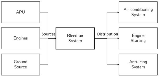
Figure 1.
Sources and functions of bleed-air systems.
The bleed-air system typically goes through intensive maintenance. In our dataset of a Boeing 737 fleet, one year registered 156 maintenance events in a fleet of 47 aircraft (3.3 actions per aircraft). Given the considerable number of aircraft based on this kind of architecture, it is essential to investigate the maintenance of these systems. In this project, we utilize data-driven (machine learning) techniques to help enhance the future maintenance of this kind of system. We hereafter explain the essential elements of a bleed system.
In bleed-air aircraft, medium- to high-pressure air is bled from the engine compressor stages. A network of ducts, sensors, valves, and regulators transfer hot and dense air from the compressor section of the engines and auxiliary power unit (APU) to various locations. The objective of the engine bleed system is to regulate the pressure and temperature of the bleed air before it is conducted into one of its final destinations.
There are two main fault modes in the bleed-air system. The first fault mode can occur when there is an extreme pressure situation. In this case, the high-pressure bleed air valve automatically locks. When this fault mode happens, the valve needs to be repaired on the ground. In the meanwhile, low air pressure continues to flow to the affected side.
The second, and the most frequent, fault mode is triggered by excessive temperature. In this situation, the corresponding engine bleed-air valve and the high-pressure bleed valve automatically close. The system can be subject to reset by turning off and on the air switch. A follow-up maintenance action is then necessary.
3.2. Data
We have two kinds of maintenance data on top of which we build our PHM models: the maintenance dataset, detailing the maintenance actions done on the system, and the sensor dataset, describing the raw data recorded along different flights:
- Maintenance event data detailing the maintenance actions performed on the system;
- Sensor data describing the raw sensor signals recorded in different flights
Regarding the maintenance event data, we have information about the maintenance actions caused by different components of the bleed-air system. Our records include two types of maintenance actions:
- Removals (repair + re-install);
- Time-scheduled maintenance interventions.
A removal happens after the identification of some anomaly. The anomaly is detected by either (i) the flight crew, (ii) a technical specialist (looking at sensor data), (iii) the aircraft itself, or (iv) an automated system. Notably, the removal dates are not necessarily the end points of degradation, i.e., some removals happen to avoid an operational disturbance later. How far the component is degraded at the moment of the removal is not registered.
It is important to note that a component might be repaired and re-installed but the problem persists. The root cause may not be immediately evident, and multiple components may be repaired at once. For example, in many cases, the sensor is removed opportunistically by taking advantage of the maintenance opportunity and not due to actual eminent functional failure. Other parts may have a fault that does not lead to an operational disturbance, so these faults can persist for a long time.
We have information about the maintenance actions that concern the following components in the bleed-air system:
- Bleed Air Check Valve
- High Stage Regulator (HSR)
- High Stage Valve (HSV)
- Precooler
- Bleed Air Regulator (BAR)
- Precooler Outlet Temperature Sensor
- Bleed Air Overtemperature Sensor
- Precooler Control Valve (PCCV)
- Isolation Valve (ISOV)
Our records have two types of maintenance actions: removals and time-scheduled interventions. A removal follows from the identification of some anomaly. This anomaly can be detected by (i) the flight crew, (ii) the technical specialist (looking at sensor data), (iii) the aircraft itself, or (iv) an automated system. Notably, the removal dates are not necessarily the ‘end-points’ of degradation, i.e., most of these removals were conducted to avoid an operational disturbance later. How far the component is degraded at the moment of removal is not known.
Importantly, a component can be removed, but the problem persists. Additionally, the root cause may not be immediately evident, and multiple components may be removed immediately. For example, in many cases, the sensor is removed opportunistically. Other components may have a fault present that does not lead to an operational disturbance (so it can persist for a long time). We also have information about engine swaps that occurred at time-fixed intervals and due to unanticipated problems.
Regarding the sensor data, the data are descriptive of around 60,000 flights (40 B737s). The data consist of 1 Hz data from all available sensors on the bleed air system, enriched by some contextual parameters, such as altitude or anti-ice settings. Generally, there are two indicators per type of parameter, one indicator for the left side bleed-air system and an equivalent indicator for the right side bleed-air system. The sensor data are anonymized, meaning that it is not possible to identify the physical meaning of each parameter.
Prior to model development, we gained some important insights into the data. The removal data were fit to a Weibull distribution, as shown in Figure 2. The parameters were estimated using the maximum likelihood estimation (MLE) method. The Weibull characteristic life parameter () estimate was 568.49 days, and the shape parameter () estimate was 1. Weibull distributions with the parameter equal to 1 have a constant failure rate, indicative of useful life or random failures. The characteristic life, , is the time at which 63.2% of the units will fail. Because , the characteristic and mean life are approximate. Note that in this analysis, we did not consider the occurrences of engine swaps or time-scheduled maintenance actions.
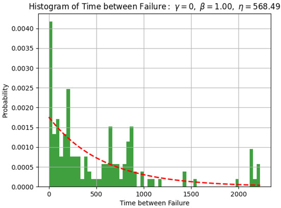
Figure 2.
Histogram of time between failures and Weibull distribution with shape parameter of 1.0 and characteristic life of 568.49 days.
4. Methods
The methods section describes the steps taken to address the research problem (Section 4.1) and the rationale for the application of specific modeling techniques (Section 4.2).
4.1. Problem Formulation
We assume the existence of m n-dimensional instances and their corresponding labels: with and . The label vector is a binary tuple that indicates for each tuple position if the instance belongs to the corresponding health state class. A health state is associated with a specific range of remaining useful life (RUL) values. For example, the most degraded health state is defined when the remaining useful life is within the range of (usage or calendar time). A second degraded health state is defined at the range .
The goal is to construct a model function that assigns a given instance point to a vector of probabilities belonging to different predefined RUL ranges (or ‘health states’). In other words, the goal is to predict the label vector corresponding to each unseen data instance. The process of learning the model from the set of training data is the training phase. On the other hand, the process of evaluating the actual performance of the modeling approach on an independent dataset of testing instances is called the testing phase.
In this problem formulation, prognostics is framed as a multiclass classification task. At each prediction time t, the system computes the probability of a continuous range of remaining useful lives. This classification is produced by observing the discrete sequence of observations up to time t denoted as . The variable of interest is the multi-label outcome of the function , where is a function of the system state and the number k of time intervals.
In contrast to binary classifiers that estimate the transition between faulty and healthy states, the target function estimates an array of probabilities of health stages. This process is illustrated in Figure 3. The input at each moment is depicted as a vertical vector of feature values. The classifier model receives these inputs and produces at each moment a multi-label probability vector, where each label corresponds to a health state (or remaining useful life range). An example list of health states with different colors is shown for a better understanding.
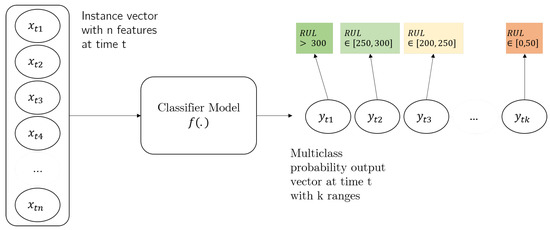
Figure 3.
General proposed framework. The classifier model receives as input a set of feature values and computes an output vector of probabilities that correspond to the likelihood of the system being in different health stages.
4.2. Modeling Approach
We follow the general prognostics flow of Figure 4, which is composed of four sub-problems: data pre-processing, condition prediction, visualization, and classification evaluation. The goal is to classify performance degradation over time to help the understanding when deterioration will reach an unacceptable level. The framework’s macro-processing steps of pre-processing, classifier, and postprocessing are hereafter described in detail.
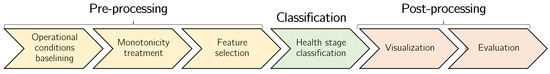
Figure 4.
The prognostics flow is composed of a number of steps, including the steps of operational condition identification and aggregation, monotonicity treatment and noise removal, and feature selection, followed by the actual health stage identification. The flow is complete after the visualization and evaluation steps.
Data Pre-Processing
The goal of data pre-processing is to obtain good features and also practical training and testing samples. This sequential process involves data baselining, monotonicity treatment (noise reduction), and feature selection.
Baselining. This is the first important step of pre-processing. Baselining is necessary because operational regimes can mask important sensory fluctuations. Degradation processes tend to cause, at some point, changes in operating parameters. These significant modifications may go undetected due to the dynamic evolution of environmental and operational conditions. Baselining (in prognostics) consists of factoring out the influence of the different operating regimes on the degradation process [34,35]. In our case, baselining is complex, as the operational conditions are unknown, and their influence on the degradation signature is not entirely evident.
The main issue in baselining is to select relevant parameters related to the system operational profile. In this case, the different flight phases of takeoff, climb, cruise, descent, and landing affect the health-monitoring signals of the engine bleed system. As shown in Figure 5, there is a marked influence of the different flight phases, easily inferred from the flying altitude, upon the condition monitoring signals. For example, during the cruise phase, the monitored blue line signal has fewer fluctuations and is more stable than in other stages, such as the landing phase. It is also noticeable that it is possible to distinguish different operating signatures, even within the same flight phase. For example, in Figure 5, it is possible to discern distinct operational regimes during takeoff.
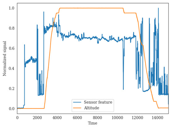
Figure 5.
The influence of the different flight phases on the condition monitoring signals. The plot shows the normalized signals of altitude and health monitoring feature for a randomly selected flight.
A regime separation scheme was developed based on the variables of flight altitude, the continuous sensory signals of interest, and the binary control parameters. The core of the algorithm is an algorithm of the kernel change-point detection that works with multidimensional data [36,37]. In general, change-point detection aims to find the boundary between samples drawn from different probability distributions. Kernel-based non-parametric statistics, such as the algorithm we use, make fewer distribution assumptions than classical parametric approaches.
The change-point detector used in our study allows us to reveal the change points that mark the transition between distinct flight phases. In particular, change point detection is used to separate the climb, cruise, and descent phases. A rule-based segmentation procedure precedes this detection. During the segmentation, a set of binary control variables is used to partition the flight altitude parameter. The Hampel filter [38] is also used to remove noisy observations from the altitude input parameter. The outcome of the baselining process is a set of operational regime labels, not necessarily equivalent to the flight phases, as flight phases, such as takeoff have more than one regime. The baselining process is graphically illustrated in the flowchart of Figure 6.
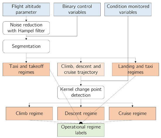
Figure 6.
Baselining flowchart. To baseline the operational data, a rule-based segmentation process is utilized on flight altitude and binary control variables. The final step consists of kernel change-point detection, based on multidimensional data that include condition monitored variables in addition to control variables and the altitude parameter to discriminate between the flight phases of the climb, cruise, and takeoff.
The baselining step results in the detection of eleven operational regimes (see Table 1), not necessarily coincident with the flight phases. Figure 7 visually shows the detection output for two randomly selected flights. The detection depends on the system behavior and the control variables. For example, the takeoff phase is partitioned into four distinct regimes, according to the fluctuations of the health parameters. Other flight phases, such as cruise or climb, are not partitioned into sub-regimes since the control variables and the health monitoring signals do not suggest the need to separate the phases further.

Table 1.
Operational regimes.
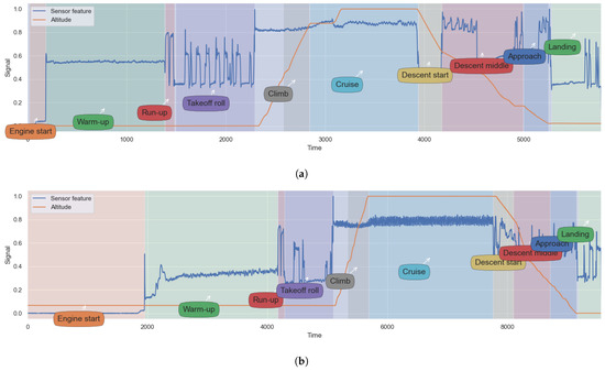
Figure 7.
Operational regimes. The figure shows randomly selected flights and their operational regimes detected during the baselining. (a) Random flight #1; (b) Random flight #2.
For each type of condition monitoring variable (e.g., temperature, pressure, and vibration), there is a left-wing and a right-wing system parameter corresponding to the aircraft’s left and right-sided engine bleed system. This redundancy is relevant, as it allows us to identify better the influence of operational conditions other than those directly related to the flight phases. Taking out the difference between the two sensor parameters within each operating regime allows factoring out these micro-regimes. Typically, when the two systems are subject to the same unexpected behavior pattern, these modifications tend not to be due to degradation-wise factors. In contrast, deterioration changes should occur more pronouncedly in a single system, and not be seen in the other system. This assumption follows from the fact that rarely are two systems under the same degradation stage.
The difference signals are aggregated per flight using the average function generating a time series for each operational regime (see list of regimes in Table 1). After aggregating all flight values, we obtain a collection of time series.
Feature engineering. We selected raw signals for the modeling approach (based on correlation). Each left-engine parameter was merged with the matching right-side engine parameter. Different summary functions were applied to convert the signals into a three-dimensional space: a dimension for each flight phase. As an illustrative example, we show in Figure 8, Figure 9 and Figure 10 a health indicator in its three dimensions. As shown, the signals are different for the different flight phases, which signals the importance of correctly distinguishing these operational phases. It is also clear from observing the signals that when a removal (or another maintenance intervention) happens, the signals indicate this change as an upward or downward jump (according to the engine side that is affected).
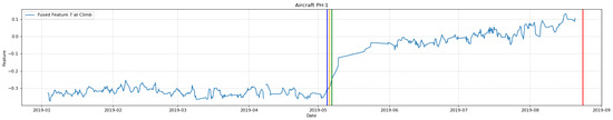
Figure 8.
Fused feature 1 at Climb of aircraft 11.
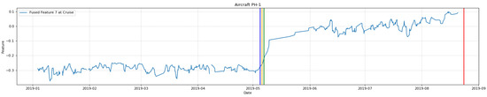
Figure 9.
Fused feature 1 at Cruise of aircraft 1.
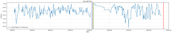
Figure 10.
Fused feature 1 at Descent of aircraft 1.
Monotonicity treatment. This step ensures the data quality since the application of monotonic constraints can act both as a feature improvement and as noise suppression [39]. We use monotonicity constraints to enforce a monotonic functional relationship between each predictor and time. The average conditional displacement (ACD) [40] is utilized to capture monotonic trends. The ACD works by approximating the signals with a piecewise linear curve. The ACD algorithm is applied independently to each interval of aircraft data between two successive failure events.
Feature selection. Better prediction results are expected in prognostics if the health indicators exhibit evident monotonic trends through the life cycle. However, it is also essential to judiciously select the most favorable set of monotonic features. In this process, we make use of the selection capabilities of random forests [41]. Random forests can compute feature importance during training. The relevance of a feature is calculated by measuring how it decreases the split criterion (Gini impurity or information gain). The average over all decision trees is used to rank features. This procedure is a simple and efficient method to obtain generally acceptable results.
4.3. Classifier Model
We follow a multiclass (or multinomial) classification approach to prognostics and health management. The aim is to classify the current health stage using a set of remaining useful life intervals. The model performs both remaining useful life estimation and health stage diagnostics. At each moment, it outputs a set of labels indicating the likelihood of the system being in a different interval of remaining useful life estimations.
We use a deep gated recurrent unit [42] to produce the multi-label forecasts. Each binary output label represents a fault classification interval or health stage. The intervals are described in Table 2. The size of the interval could be different. The rationale behind the selection is to balance the data whilst obtaining industrial meaning. The interval size has to be large enough to capture several equipment in the early stages. For example, imagine that some equipment lasted y days, other days. The larger the interval size, the better we accommodate the lack of data in the first x days of the equipment that only lasts y days. On the contrary, two large intervals do not convey as much meaning to the industrial operator as needed. The intervals were defined to be of an equal length of 50 days. Calendar time (days) was utilized to determine the intervals instead of usage time (e.g., number of cycles) because many flights were incorrectly recorded or not recorded for long periods, which hindered the second type of analysis. The period of 50 days was considered to be an acceptable period. We selected these value based on experiments with the data and the model.
Table 2.
Health stages.
4.3.1. Recurrent Neural Networks
Recurrent neural networks are a class of neural networks with internal mechanisms to model and regulate the flow of historical information. While processing, these networks transfer the previous hidden state to the next computation step of the training process. The hidden state acts as neural network memory. It maintains information about the previous data seen by the network. Applications of recurrent neural techniques can be found in speech recognition [43,44], language models [45,46], and text generation [47] for example.
In prognostics, these models are often used to estimate the remaining useful life of the equipment, as they allow capturing the temporal dimension of the sensor data. There are different types of recurrent neural networks, such as the long short-term memory (LSTM) network introduced by Hochreiter and Schmidhuber [48] and the gated recurrent unit (GRU) proposed more recently by [42], standing as the most popular approaches. In this work, we explore the GRU capabilities, as this approach excels at processing long sequences quickly. GRU is similar to LSTM, but this network belongs to a newer generation of recurrent networks with only two gates, the reset and update gates. This simplification reduces the complexity of the network. Additionally, GRU has fewer parameters than other recurrent nets, so training is faster and fewer data are needed to generalize the model.
The proposed prognostics model is a GRU with several layers (see Figure 11). The first layer is the input layer (in grey color) that receives and keeps the vectors that represent the measurements at each time instant. Next are the GRU layers (in light blue). These layers are responsible for deep learning computation and for managing the network memory. The output layer must create seven output labels, one for each health stage indicator. Because we frame prognostics as a multiclass classification problem, the activation function is softmax [49], and categorical cross-entropy [50] is used as the loss function.
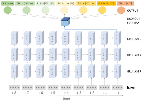
Figure 11.
Deep gated recurrent unit (GRU) multiclass classification model. The prognostics is performed using a GRU model that classifies the different health stages of the equipment. Each health stage represents a range of possible remaining useful life values.
A dropout layer (in dark blue) is applied to help the network generalize better. The network is stateful, meaning that all the states are propagated to the next batch. If the network was stateless, parameters would be calculated for one batch, and then hidden states and cell states would be set to zero for the next batch. There is a connection between batch learning in stateful nets since the batch’s final states are used as initial states for the subsequent batch. In this way, we are exposing the network to the entire sensor data to promote better learning of the inter-dependencies of the sequences.
4.3.2. Model Optimization
In this work, we use a genetic algorithm (GA) [51] for finding the near-optimal parameters of the gated recurrent unit (GRU). Genetic algorithms are often used to deal with optimization problems. They can help obtain a fast and approximate solution of a complex problem. As stated by Dracopoulos and Dracopoulos [52], “genetic algorithms are often used in machine learning tasks in the form of classifier systems”. Since our focus was not to test GA variants, we used the classical GA algorithm [51].
We used the GA to optimize the hyper-parameters of the neural network, such as learning rate, number of neurons, and window size (see Table 3) The GA used in this work implements the three basic operations of selection, to define which solutions to preserve, the crossover, to derive new solutions from existing ones, and mutation, to introduce diversity into the solution pool employing binary mutation. Figure 12 depicts the structure of the used genetic algorithm. The initial solutions (population) are randomly generated. The fitness function is the macro-average area under the curve (AUC) score. The macro-average AUC was preferred over the micro-average AUC since the model had lower performance on this first dimension.
Table 3.
Range and hyperparameters tested by the genetic algorithm.
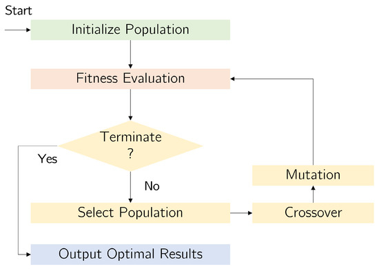
Figure 12.
Basic logic of genetic algorithm.
4.4. Visual Assessment
While preparing the data and building models are key steps of prognostics, it is also important to analyze the quality of the predictions using metrics and visual indicators. Before using the algorithms to optimize a maintenance team’s repair schedules and long-term plans, testing and evaluating the model output from distinct performance dimensions is necessary.
In prognostics, visual tools for evaluation are often neglected over numerical performance indicators [53,54]. Even though it is essential to have a quantitative analysis of the results, having visual aids to help the maintainer quickly investigate what is happening with the equipment is of central value. This necessity is especially true for data-driven models, such as our proposed neural network. Due to the black-box nature of these networks, it is important to go beyond common evaluation metrics to understand in full detail the actual performance and limitations of this kind of prognostics model.
We propose two visual assessment tools: the prognostics ROC curve and the risk plots. It is important to remember the basics of evaluating classification models. Typically, the classifier evaluation metrics are built from the confusion matrix [55].
Table 4 presents the scheme of a confusion matrix for a 2-class classifier [56]. In our model, a true positive (TP) occurs when the predictive indicator for the actual RUL range is above its decision criterion, and a true negative (TN) when the negative label is below its decision criterion. In contrast, false positives (FP) and false negatives (FN) happen when the predicted RUL range does not match the true RUL range. With this matrix, the performance of each predictive indicator can be measured on the dimensions of sensitivity, specificity, precision, accuracy, recall and F1-score [57]:
Table 4.
Confusion matrix scheme.
Sensitivity or recall concerns the ability to predict the different health stages correctly. Specificity assesses how accurately the model predicts that the equipment is not yet at that health stage (RUL interval). Precision is a function of true positives and false positives. Accuracy is the ratio of well-predicted and incorrectly predicted samples. The F1-score measures precision and recall.
4.4.1. Receiver Operating Characteristic Curve
The receiver operating characteristic (ROC) curve is a visual tool to help assess the quality of the classification. It relates the fraction of true-positive samples (sensibility) and the fraction of false-positive samples (1-specificity) as the decision criterion (or likelihood threshold) changes [58]. ROC curves are typically used in binary classification but can be extended to multi-label classification. One ROC curve can be drawn per class (RUL range or health stage) by considering each element of the different confusion matrices. The ROC curve can be calculated using the micro-average or the macro-average methods. In micro-averaging, we first sum all the elements of the different confusion matrices and then apply the statistics. In macro-averaging, we take the average of the statistics of different classes. The difference between macro- and micro-averaging is that the macro scheme weighs each class equally, whereas the micro scheme weighs each sample equally. Micro-averaging is suitable if the data are imbalanced, while the macro-average is convenient to verify if there is no large class dominating the prediction.
4.4.2. Risk Plot
The risk plot is another visual tool specific to each interval between two maintenance events, either a removal (repair + re-install) or a scheduled maintenance intervention. The goal of a risk plot is to depict the evolution of the different class indicators over time. The risk plot features on the x-axis the time, from the starting point to the end-of-life of the equipment, and on the y-axis, the likelihood of the different health stage (risk) indicators. The desirable behavior would be to have each indicator at the highest risk only between the boundaries of its RUL range. The vertical boundaries are also drawn in the risk plot for a better visual understanding of the predictions. Examples of risk plots will be given in the next section.
5. Results
In this section, we evaluate the performance of the prognostics pipeline. Details about the experimental setup are provided, and results are presented and discussed.
5.1. Research Question
This study focuses on a single research hypothesis, which is tested on the Boeing 737 data described in Section 3. The hypothesis reads as follows:
Multiclass models based on the gated recurrent unit (GRU) neural network can achieve a macro-average area and micro-average area under the model’s ROC curve (AUC) above 50%.
5.2. Confusion Matrix
Figure 13 shows the resulting confusion matrix. The matrix compares the actual target values, i.e., the actual RUL ranges, with those predicted by the GRU model. The matrix gives a comprehensive view of the model and its limitations. It can be seen that the number of correctly predicted data points in the most safety critical class, near the end of life (label of range ), is above 55%.
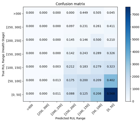
Figure 13.
Multiclass confusion matrix. The 7 × 7 confusion matrix allows us to evaluate the performance of the GRU classification model, whereby 7 is the number of target classes.
There is, however, a marked tendency to misclassify items in this category. Still, there is a considerable portion of instances (20.9%, 18.3% and 14.2%) that are correctly classified in the ranges of , and . It is noticeable how the accuracy diminishes as we get away from the equipment’s end of life. This result is understandable since the equipment shows increased signs of degradation as we get closer to the end of life. Consequently, it is easier to predict the actual remaining useful life at the latest health stage.
5.3. Multiclass Receiver Operating Characteristics Curve
To plot the receiver operating characteristics (ROCs) curves of the different classes, we follow the methodology of using one class versus the rest. Following this method, the ROC curves and the area under the ROC curve (AUC) scores are calculated individually by converting each class into a binary problem. The multiclass ROC plot is a valuable tool for evaluating the quality of class separation.
In Figure 14, we have the ROC plot of the GRU model. As shown, the micro-average AUC score is significantly high at 0.72. In turn, the macro-average AUC score is only 0.52. An analysis of the different ROC curves shows that the less safety critical indicators were responsible for such a low macro-average AUC score. While the AUC scores of the most safety critical ROC curves were consistently above the 0.50 values (except for the [50, 100] class), the >300 curve had a low AUC score of 0.34. This result could explain why the average of all ROC curves resulted in a low micro-average AUC score. This result suggests that issues related to imbalanced data could have affected the prediction.
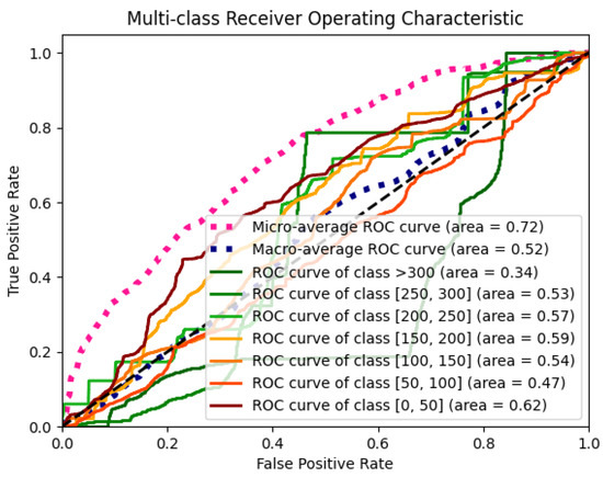
Figure 14.
Multiclass receiver operating characteristics (ROC) curve.
5.4. Precision–Recall Plot
The precision–recall plot is utilized to perform a model-wide evaluation using the measures of recall and precision (and F1-score). As can be seen in Figure 15, the best performing indicator is the most safety critical one (Class 6 in dark red) with an average precision (AP) score of 0.51. This is a positive result, as it indicates that the most dangerous state tends to be correctly anticipated. The low AP scores of the healthiest stage indicators (green indicators) suggest that the model lost accuracy when predicting these calendar intervals.
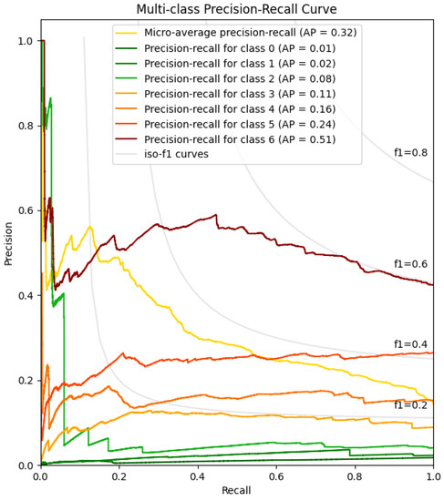
Figure 15.
Multiclass precision–recall plot.
As a complex system with components at different degradation levels, the engine bleed system is difficult to predict. It is problematic to indicate the actual state of health 300 or 200 days away from the end of life. This fact might explain the poor performance of the model as it moves near the previous repair action. The best approach to mitigate the lack of accuracy would be to have more data and to develop more informative features that could help understand the degradation stage early on.
5.5. Risk Plots
The risk plots shown in Figure 16 are promising. As can be seen in the different charts, the indicators are connected in time, i.e., the prediction at one time is based on the previous forecast. Instead of scattered predictions, we have visually appealing indicators that follow clear trends. This is a positive result that can be explained by the use of the GRU. Since the GRU is a recurrent neural network, the model considers the temporal aspect, with each prediction considering the current state and network memory.
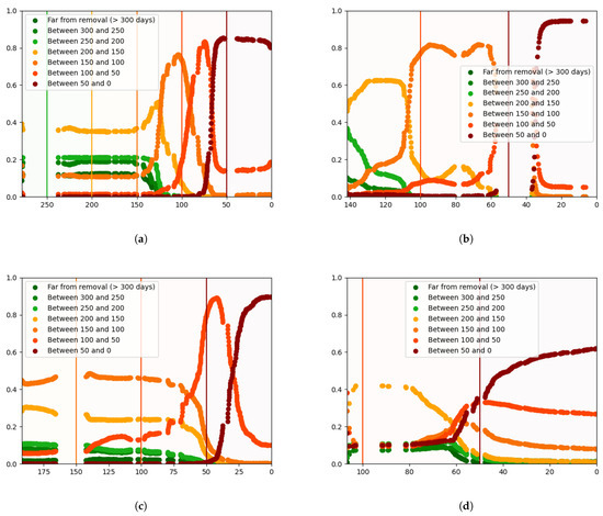
Figure 16.
Risk plots. The risk plot shows the progress of the health stage indicators over the life of four equipment units. Each of these plots shows the predictions of the GRU model over the life of an equipment. (a) Random Equipment #1; (b) Random Equipment #2; (c) Random Equipment #3; (d) Random Equipment #4.
Sometimes, the indicators do not start at the exact time that they were expected to begin. For example, in Figure 16a, the most critical indicator (in dark red) starts about ten days earlier than expected. In Figure 16b, the same indicator starts to rise around ten days later.
Another example is the indicator of (in red). This indicator is sometimes predicted within the range of as shown in Figure 16c. These inaccuracies are detrimental to the model’s global performance, but they do not necessarily hinder the utility of the results. When far away from the end of life, the human operator needs to have a broad notion of when the failure will happen. The operator only needs to know in very general terms when the failure will happen in order to proceed with the maintenance scheduling and design its future maintenance plans. Put differently, it is not critical to have some degree of uncertainty in the estimates far from the end of life as long as these estimates become increasingly accurate as they are updated as time changes.
An explanation for the inaccuracies is that it may be difficult to distinguish the calendar-time health intervals in physics-of-failure terms. Degradation-wise, we may be at the same degradation level when we are at 50 days away from the end of life for the equipment in Figure 16a, as when we are 40 days away from the end of life for the equipment in Figure 16b. The time intervals do not necessarily express degradation intervals.
Even if it was possible to model the usage time (e.g., by the number of cycles) instead of calendar time, the same issue could arise since degradation often depends on other factors, which are not the (usage/calendar) time. These results suggest it will be important to set up the class intervals in a more dynamic and sophisticated manner. In other words, it would be more beneficial to have a way to quantify the actual degradation of the component and try to predict the fundamental degradation stages, and not only the temporal stages.
5.6. Summary
Given these results, we believe that we found sufficient evidence to support our hypothesis (see Section 5.1). It is possible to achieve good performance in fault prognostics using multiclass classifier approaches. Our findings also suggest that it might be beneficial to establish the model classes in a different way, either exploring usage time or a degradation-wise indicator.
6. Conclusions
In this paper, a novel approach to prognostics based on multiclass classification was proposed. This work aims to provide an alternative approach to prognostics that is not based on remaining useful life (RUL) estimation methods. Instead of the remaining useful life prediction, we propose to relax the precision requirements by developing a solution that is more in line with an aerospace engineering team’s visual and analytic needs. The proposed model does not predict RUL estimates but instead, the indication of a range of possible RUL values at each moment. The problem of prognostics is framed as a classification data-driven task, rather than a regression task. Ultimately the aim is to provide valuable and clear information to help industry experts develop their scheduling and planning schemes.
To a certain extent, it may even be easier to interpret and manage a collection of health state indicators than to deal with an array of (often conflicting) numerical estimates. Humans do not deal exceptionally well with numbers. They tend to prefer risk indicators and visually informative plots. Our goal with this work is to prevent the maintenance operator from working directly with numbers. The operator should base his or her decisions on visual tools and simplified dashboards instead. The operator monitors several components in a real-world scenario and could benefit from a decision support system based on more interpretable prognostics models. Our proposed multiclass classification model aims to be a major step in that direction.
A wide range of metrics and tools can be used to analyze and evaluate the quality of multiclass classification models. The confusion matrix, receiver operating characteristic (ROC) curve, precision–recall plot, risk plots, and others [59] are suitable alternatives. A large community is working on new assessment methods for multiclass classification methods that could be applied and utilized by the prognostics and health management (PHM) community. With better performance of the models, we also obtain more interpretable prognostics. Confidence and trust can only be built from models that are correctly evaluated in a multi-perspective view.
In the future, we intend to study how to set the model intervals in a way that allows us to generate better predictions, and to more accurately model the component degradation states. Our future work will explore and combine the GRU model with other advanced deep learning models, such as convolution neural networks and auto-encoders. Finally, we aim to adapt existing evaluation metrics for these models as well as proposing new ones.
Author Contributions
Conceptualization, M.L.B.; methodology, M.L.B.; software, M.L.B.; validation, M.L.B. and H.P.; formal analysis, M.L.B.; investigation, M.L.B.; writing—original draft preparation, M.L.B.; writing—review and editing, M.L.B. and H.P. All authors have read and agreed to the published version of the manuscript.
Funding
This research received no external funding.
Institutional Review Board Statement
Not applicable.
Informed Consent Statement
Not applicable.
Data Availability Statement
Not applicable.
Conflicts of Interest
The authors declare no conflict of interest.
References
- Xu, Z.; Saleh, J.H. Machine learning for reliability engineering and safety applications: Review of current status and future opportunities. Reliab. Eng. Syst. Saf. 2021, 211, 107530. [Google Scholar] [CrossRef]
- Zio, E. Prognostics and Health Management (PHM): Where are we and where do we (need to) go in theory and practice. Reliab. Eng. Syst. Saf. 2022, 218, 108119. [Google Scholar] [CrossRef]
- Zio, E. Reliability engineering: Old problems and new challenges. Reliab. Eng. Syst. Saf. 2009, 94, 125–141. [Google Scholar] [CrossRef]
- Goebel, K.; Daigle, M.; Saxena, A.; Sankararaman, S.; Roychoudhury, I.; Celaya, J. Prognostics: The Science of Making Predictions, 1st ed.; CreateSpace Independent Publishing Platform: Scotts Valley, CA, USA, 2017. [Google Scholar]
- Tamilselvan, P.; Wang, P. Failure diagnosis using deep belief learning based health state classification. Reliab. Eng. Syst. Saf. 2013, 115, 124–135. [Google Scholar] [CrossRef]
- Niu, G.; Yang, B.S.; Pecht, M. Development of an optimized condition-based maintenance system by data fusion and reliability-centered maintenance. Reliab. Eng. Syst. Saf. 2010, 95, 786–796. [Google Scholar] [CrossRef]
- Baraldi, P.; Razavi-Far, R.; Zio, E. Classifier-ensemble incremental-learning procedure for nuclear transient identification at different operational conditions. Reliab. Eng. Syst. Saf. 2011, 96, 480–488. [Google Scholar] [CrossRef]
- Li, Z.; Wu, D.; Hu, C.; Terpenny, J. An ensemble learning-based prognostic approach with degradation-dependent weights for remaining useful life prediction. Reliab. Eng. Syst. Saf. 2019, 184, 110–122. [Google Scholar] [CrossRef]
- ISO13381-1:(e); Diagnostics of Machines-Prognostics Part 1: General Guidelines. Technical Committee: ISO/TC 108/SC 5 Condition Monitoring and Diagnostics of Machine Systems; ISO: Geneva, Switzerland, 2004; p. 14.
- Daigle, M.J.; Goebel, K. A Model-based Prognostics Approach applied to Pneumatic Valves. Int. J. Progn. Health Manag. 2011, 2, 84–99. [Google Scholar]
- Fink, O.; Zio, E.; Weidmann, U. Predicting component reliability and level of degradation with complex-valued neural networks. Reliab. Eng. Syst. Saf. 2014, 121, 198–206. [Google Scholar] [CrossRef]
- Ramasso, E. Contribution of belief functions to hidden markov models with an application to fault diagnosis. In Proceedings of the 2009 IEEE International Workshop on Machine Learning for Signal Processing, Grenoble, France, 1–4 September 2009. [Google Scholar] [CrossRef]
- Saxena, A.; Goebel, K.; Simon, D.; Eklund, N. Damage propagation modeling for aircraft engine run-to-failure simulation. In Proceedings of the 2008 International Conference on Prognostics and Health Management, Denver, CO, USA, 6–9 October 2008. [Google Scholar] [CrossRef]
- Ramasso, E.; Denoeux, T. Making Use of Partial Knowledge About Hidden States in HMMs: An Approach Based on Belief Functions. IEEE Trans. Fuzzy Syst. 2014, 22, 395–405. [Google Scholar] [CrossRef]
- Ramasso, E.; Gouriveau, R. Remaining Useful Life Estimation by Classification of Predictions Based on a Neuro-Fuzzy System and Theory of Belief Functions. IEEE Trans. Reliab. 2014, 63, 555–566. [Google Scholar] [CrossRef]
- Peng, Y.; Wang, H.; Wang, J.; Liu, D.; Peng, X. A modified echo state network based remaining useful life estimation approach. In Proceedings of the 2012 IEEE Conference on Prognostics and Health Management, Denver, CO, USA, 18–21 June 2012. [Google Scholar] [CrossRef]
- Javed, K.; Gouriveau, R.; Zemouri, R.; Zerhouni, N. Features Selection Procedure for Prognostics: An Approach Based on Predictability. IFAC Proc. Vol. 2012, 45, 25–30. [Google Scholar] [CrossRef]
- Kim, H.E.; Tan, A.C.C.; Mathew, J. New machine prognostics approach based on health state probability estimation. Aust. J. Mech. Eng. 2011, 8, 79–89. [Google Scholar] [CrossRef]
- de Padua Moreira, R.; Nascimento, C.L. Prognostics of aircraft bleed valves using a SVM classification algorithm. In Proceedings of the 2012 IEEE Aerospace Conference, Big Sky, MO, USA, 3–10 March 2012. [Google Scholar] [CrossRef]
- Louen, C.; Ding, S.X.; Kandler, C. A new framework for remaining useful life estimation using Support Vector Machine classifier. In Proceedings of the 2013 Conference on Control and Fault-Tolerant Systems (SysTol), Nice, France, 9–11 October 2013. [Google Scholar] [CrossRef]
- Castilho, H.M.; Nascimento, C.L.; Vianna, W.O.L. Aircraft bleed valve fault classification using support vector machines and classification trees. In Proceedings of the 2018 Annual IEEE International Systems Conference (SysCon), Vancouver, BC, Canada, 23–26 April 2018. [Google Scholar] [CrossRef]
- Allegorico, C.; Mantini, V. A data-driven approach for on-line gas turbine combustion monitoring using classification models. In Proceedings of the PHM Society European Conference, Nantes, France, 8–10 July 2014; Volume 2. [Google Scholar]
- Liu, C.L.; Hsaio, W.H.; Tu, Y.C. Time Series Classification With Multivariate Convolutional Neural Network. IEEE Trans. Ind. Electron. 2019, 66, 4788–4797. [Google Scholar] [CrossRef]
- Li, K.; Wu, Y.; Nan, Y.; Li, P.; Li, Y. Hierarchical multi-class classification in multimodal spacecraft data using DNN and weighted support vector machine. Neurocomputing 2017, 259, 55–65. [Google Scholar] [CrossRef]
- Shen, F.; Chen, C.; Yan, R.; Gao, R.X. Bearing fault diagnosis based on SVD feature extraction and transfer learning classification. In Proceedings of the 2015 Prognostics and System Health Management Conference (PHM), Beijing, China, 21–23 October 2015. [Google Scholar] [CrossRef]
- Wang, P.; Tamilselvan, P.; Hu, C. Health diagnostics using multi-attribute classification fusion. Eng. Appl. Artif. Intell. 2014, 32, 192–202. [Google Scholar] [CrossRef]
- Lall, P.; Gupta, P.; Angral, A. Anomaly Detection and Classification for PHM of Electronics Subjected to Shock and Vibration. IEEE Trans. Compon. Packag. Manuf. Technol. 2012, 2, 1902–1918. [Google Scholar] [CrossRef]
- Li, X.; Zhang, W.; Ma, H.; Luo, Z.; Li, X. Deep learning-based adversarial multi-classifier optimization for cross-domain machinery fault diagnostics. J. Manuf. Syst. 2020, 55, 334–347. [Google Scholar] [CrossRef]
- Baptista, M.L.; Henriques, E.M.; Prendinger, H. Classification prognostics approaches in aviation. Measurement 2021, 182, 109756. [Google Scholar] [CrossRef]
- Janasak, K.; Beshears, R. Diagnostics To Prognostics—A Product Availability Technology Evolution. In Proceedings of the 2007 Proceedings—Annual Reliability and Maintainability Sympsoium, Orlando, FL, USA, 22–25 January 2007. [Google Scholar] [CrossRef]
- Zein-Sabatto, S.; Bodruzzaman, M.; Mgaya, R.; Behbahani, A. Distributed Onboard Diagnostic Methodology for Next Generation Turbine Engines. In Proceedings of the 46th AIAA/ASME/SAE/ASEE Joint Propulsion Conference Exhibit. American Institute of Aeronautics and Astronautics, Nashville, TN, USA, 25–28 July 2010. [Google Scholar] [CrossRef]
- Kumar, A.; Chinnam, R.B.; Tseng, F. An HMM and polynomial regression based approach for remaining useful life and health state estimation of cutting tools. Comput. Ind. Eng. 2019, 128, 1008–1014. [Google Scholar] [CrossRef]
- Sebok, M. Condition Analysis of Electrical Machines by Thermovision. Przegląd Electhrotecknizny 2020, 1, 49–52. [Google Scholar] [CrossRef]
- Zhang, J.; Jiang, N.; Li, H.; Li, N. Online health assessment of wind turbine based on operational condition recognition. Trans. Inst. Meas. Control 2018, 41, 2970–2981. [Google Scholar] [CrossRef]
- Baptista, M.L.; Henriques, E.M.P.; Goebel, K. A self-organizing map and a normalizing multi-layer perceptron approach to baselining in prognostics under dynamic regimes. Neurocomputing 2021, 456, 268–287. [Google Scholar] [CrossRef]
- Celisse, A.; Marot, G.; Pierre-Jean, M.; Rigaill, G. New efficient algorithms for multiple change-point detection with reproducing kernels. Comput. Stat. Data Anal. 2018, 128, 200–220. [Google Scholar] [CrossRef]
- Arlot, S.; Celisse, A.; Harchaoui, Z. A kernel multiple change-point algorithm via model selection. J. Mach. Learn. Res. 2019, 20, 1–56. [Google Scholar]
- Pearson, R.K.; Neuvo, Y.; Astola, J.; Gabbouj, M. The class of generalized hampel filters. In Proceedings of the 2015 23rd European Signal Processing Conference (EUSIPCO), Nice, France, 31 August–4 September 2015. [Google Scholar] [CrossRef]
- Coble, J.; Hines, J.W. Identifying Suitable Degradation Parameters for Individual-Based Prognostics. In Diagnostics and Prognostics of Engineering Systems; IGI IGI Global: Hershey, PA, USA, 2013; pp. 135–150. [Google Scholar] [CrossRef]
- Vamos, C.; Craciun, M. Automatic Trend Estimation; Springer: Berlin/Heidelberg, Germany, 2013. [Google Scholar] [CrossRef]
- Breiman, L. Random forests. Mach. Learn. 2001, 45, 5–32. [Google Scholar] [CrossRef]
- Cho, K.; van Merrienboer, B.; Gulcehre, C.; Bahdanau, D.; Bougares, F.; Schwenk, H.; Bengio, Y. Learning Phrase Representations using RNN Encoder–Decoder for Statistical Machine Translation. In Proceedings of the 2014 Conference on Empirical Methods in Natural Language Processing (EMNLP), Doha, Qatar, 25–29 October 2014. [Google Scholar] [CrossRef]
- Lee, J.; Tashev, I. High-level feature representation using recurrent neural network for speech emotion recognition. In Proceedings of the ISCA Interspeech 2015, Dresden, Germany, 11 September 2015. [Google Scholar] [CrossRef]
- Chien, J.T.; Shen, C. Stochastic Recurrent Neural Network for Speech Recognition. In Proceedings of the ISCA Interspeech 2017, Stockholm, Sweden, 20–24 August 2017. [Google Scholar] [CrossRef]
- Mikolov, T.; Karafiát, M.; Burget, L.; Černocký, J.; Khudanpur, S. Recurrent neural network based language model. In Proceedings of the ISCA Interspeech 2010, Chiba, Japan, 26–30 September 2010. [Google Scholar] [CrossRef]
- Morioka, T.; Iwata, T.; Hori, T.; Kobayashi, T. Multiscale recurrent neural network based language model. In Proceedings of the Interspeech 2015, Dresden, Germany, 11 September 2015. [Google Scholar] [CrossRef]
- Shini, R.S.; Kumar, V.A. Recurrent Neural Network based Text Summarization Techniques by Word Sequence Generation. In Proceedings of the IEEE 2021 6th International Conference on Inventive Computation Technologies (ICICT), Coimbatore, India, 20–22 January 2021. [Google Scholar] [CrossRef]
- Hochreiter, S.; Schmidhuber, J. Long Short-Term Memory. Neural Comput. 1997, 9, 1735–1780. [Google Scholar] [CrossRef] [PubMed]
- Wang, J.; Zhan, C.; Yu, D.; Zhao, Q.; Xie, Z. Rolling bearing fault diagnosis method based on SSAE and softmax classifier with improved K-fold cross-validation. Meas. Sci. Technol. 2022, 33, 105110. [Google Scholar] [CrossRef]
- Koidl, K. Loss Functions in Classification Tasks. P.hD. Thesis, School of Computer Science and Statistic Trinity College, Dublin, Ireland, 2013. [Google Scholar]
- Mirjalili, S. Genetic Algorithm. In Studies in Computational Intelligence; Springer International Publishing: Berlin/Heidelberg, Germany, 2018; pp. 43–55. [Google Scholar] [CrossRef]
- Dracopoulos, D.C.; Dracopoulos, D.C. Genetic algorithms. In Evolutionary Learning Algorithms for Neural Adaptive Control; Springer: London, UK, 1997; pp. 111–131. [Google Scholar]
- Saxena, A.; Celaya, J.; Saha, B.; Saha, S.; Goebel, K. Evaluating algorithm performance metrics tailored for prognostics. In Proceedings of the 2009 IEEE Aerospace Conference, Big Sky, MO, USA, 7–14 March 2009. [Google Scholar] [CrossRef]
- Goebel, K.; Saxena, A.; Saha, S.; Saha, B.; Celaya, J. Prognostic Performance Metrics. In Machine Learning and Knowledge Discovery for Engineering Systems Health Management; Chapman and Hall/CRC: Boca Raton, FL, USA, 2016; pp. 147–177. [Google Scholar] [CrossRef]
- Japkowicz, N.; Shah, M. Evaluating Learning Algorithms: A Classification Perspective; Cambridge University Press: Cambridge, UK, 2011. [Google Scholar]
- Kohavi, R.; Provost, F. On applied research in machine learning. Appl. Mach. Learn. Knowl. Discov. Process 1998, 30, 127–132. [Google Scholar]
- Sokolova, M.; Japkowicz, N.; Szpakowicz, S. Beyond accuracy, F-score and ROC: A family of discriminant measures for performance evaluation. In Proceedings of the Australasian Joint Conference on Artificial Intelligence; Springer: Berlin/Heidelberg, Germany, 2006; pp. 1015–1021. [Google Scholar]
- Fawcett, T. An introduction to ROC analysis. Pattern Recognit. Lett. 2006, 27, 861–874. [Google Scholar] [CrossRef]
- Tharwat, A. Classification assessment methods. Appl. Comput. Inform. 2020, 17, 168–192. [Google Scholar] [CrossRef]


Disclaimer/Publisher’s Note: The statements, opinions and data contained in all publications are solely those of the individual author(s) and contributor(s) and not of MDPI and/or the editor(s). MDPI and/or the editor(s) disclaim responsibility for any injury to people or property resulting from any ideas, methods, instructions or products referred to in the content. |
© 2023 by the authors. Licensee MDPI, Basel, Switzerland. This article is an open access article distributed under the terms and conditions of the Creative Commons Attribution (CC BY) license (https://creativecommons.org/licenses/by/4.0/).