Adaptive Division and Analysis Data Extraction of Air-Cooled Turbine Blade for Pipe Network Calculation

Abstract

Manually preparing the data for the analysis of the calculation of a pipe network of air-cooled turbine blades is inefficient. In this paper, a method to adaptively divide the blade model and extract data of the flow units is proposed. In this method, the topological lines of the flow channels for the calculations of the pipe network were extracted based on the simulatedfluid flow. The abstracted lines of the fluid flow area were used to replace the manual interpretation of expertsto realize the adaptive division of the flow units and to understand the connection relationship of the units and the layout of the spatial network. In addition, by establishing a basic flow unit library and constructing a specific algorithm, we quickly extracted the data from the typical flow units. Finally, the proposed method and algorithm were verified with a representative case study. The results illustrated that our method could cut down the pre-processing in the calculation of the pipe network of air-cooled turbine blades to several minutes from the several hours required for the manual method while providing reliable quality.

1. Introduction

Turbine blades are the key components of aero-engines, which must work under high-speed, high-temperature, and high-pressure conditions for a long amount of time. The gas temperature in front of a turbine is much higher than the temperature tolerance range of the materials commonly used for blades [1]. To ensure the blades’ safe operation and endurance, a composite cooling technology is generally used in the structural design to cool the blades [2,3,4,5]. The design quality and efficiency of the cooling technology of the blades have an impact on the thrust-weight ratio and development cycle of aero-engines.

Accurately predicting the temperature field of turbine blades is the key to improving the cooling efficiency and prolonging the working life of the blades. Obtaining the heat transfer data through experimental measurement is difficult and results in the high cost of the experiment and requires a long cycle. Therefore, one of the most commonly used methods to obtain heat transfer data is to simulate alternative turbine cooling schemes by a numerical calculation, selecting the optimal scheme and, then, conducting an experimental verification. However, the calculations in a three-dimensional (3D) simulation are usually time-consuming and require much computing power. Hence, empirical formulas using a one-dimensional (1D)/two-dimensional (2D) heat transfer design of the blades are an alternative method of calculation commonly used in engineering design and scientific research [6,7,8]. This method does not rely on commercial software; the iteration speed of the calculation is fast, and the rationality of the cooling channel design scheme can be quickly checked under the existing heat transfer data preparation conditions.

Pipe network calculation (PNC), also called fluid network calculation, is a 1D numerical method that extracts the major essential factors from a complex flow and generalizes them to a model of a network system consisting of nodes and components [9]. While the calculation accuracy of pipe network analysis may be less than that of a 3D numerical calculation because of the simplification to one dimension, because an empirical correlation [10,11] is used in the pipe network calculation, the results are very reliable. Additionally, due to its rapid calculation (about 1∼2 min) and high efficiency, applying PNC to the preliminary stage of a schematic design holds great significance [12,13,14].

Generally, the research on PNC has focused on the flow of heat, such as the mechanism for the cooling elements [15], the selection of the empirical formulas and parameters [16], the design and optimization of the solver [17], the application of PNC to the design of a blade system [18,19,20,21,22], the optimization and design of different types of air-cooled blades [23,24,25], etc. The PNC process consists of three main steps: (1) the pre-processing, (2) the solver, and (3) the post-processing steps. Among these, the pre-processing stage is the most time-consuming part because of the preparation of a large amount of data and the visual representation of the model of the topological relations [26,27,28]. Therefore, some scholars have attempted to develop suitable methods and programming to manipulate the geometry of the blades to realize the automation of the pre-processing step in PNC. Wang Songtao et al. [29] developed a multilevel cooling structure design process that takes advantage of pipe network analysis and 3D conjugate heat transfer simulations. The platform can not only provide a design guide, as well as highly accurate thermal calculations, but it can also obtain the geometry model’s parameters and automatically mesh them, thereby significantly reducing the design time.

Commonly, there are three main stages in the pro-precessing of the PNC: (1) the division of the flow units, (2) the extraction of the geometric data and physical properties of the flow units, and (3) the formation of the network topology for the PNC. Fu et al. [30] presented a method for the extraction of the heat transfer data to analyze an air-cooled turbine blade model, including the algorithms for computing the division of the units, the automatic determination of the air path, the generation of the network diagram, and the automatic extraction of the heat transfer data for the analysis. In this method, the flow units are obtained by cutting the blade body into a set of longitudinal planes and a set of transverse planes. The planes are defined by manually entering the parameters. Hence, adjusting the planes to generate suitable flow units represents the most demanding and repetitive work of the method. For the extraction of geometric data for specific components, Li et al. [31,32] investigated a method to extract the parameters from the geometric structure of film holes. Owing to a large number of gas film holes, the manual configuration of the parameter of the film hole components would affect the efficiency of the PNC. The method includes two key steps: (1) the grouping of the film holes and (2) the extraction of the parameters for the numerical analysis. This converts the requirements of the fluid-heat analysis into a geometric row pattern recognition problem and further redefines the geometric row as a linear distribution by a projection method. The extraction of the parameters redefines the parameters to be analyzed as geometric properties and identifies certain geometry primitives.

In the pre-processing of the PNC, the flow units need to be divided according to the solid model of the blades, the geometric data and the physical properties of the flow units need to be manually extracted, and the network topology needs to be formed according to the connection relationship of the flow units. However, there are still some problems that need to be solved in the overall pre-processing stage. (1) The division of flow units is cumbersome, and the standards have not been unified. (2) The data configuration of the flow units for the calculation is cumbersome and error-prone. (3) The manual drawing of the network diagram requires the manual input of the unit data.

These all seriously affect the efficiency of the design-analysis iterations and the quality of the analysis of the blades. At the same time, the pipe network model for the manual configuration of the data and the network diagram does not meet the automation requirements of CAD software and the heat transfer analysis of the solution for the blades.

Aiming at the above problems, a method to extract the topological lines for the pipe network computation based on fluid flow simulationsis proposed in this paper. This method uses the abstract lines of the fluid flow area to replace the manual determination by experts, realizing the adaptive division of the pipeline network computational units based on the topological line, the determination of the connectivity relationship of the flow units, and the layout of the spatial network units. At the same time, a data transmission mechanism was constructed using the flow units, the extracted data, and topological network diagrams to improve the accuracy and efficiency of the PNC.

The rest of this paper is organized as follows. Section 2 briefly introduces the scheme for constructing the flow heat pipe network model. Section 3 presents the adaptive division of the turbine blade model based on the topological lines of the pipe network. Section 4 presents the method to construct the pipe network topology diagram. The flow unit data extraction method is shown in Section 5. Moreover, Section 6 gives some representative examples. Finally, Section 6 concludes this paper.

2. Scheme of Constructing Flow Heat Pipe-Network Model

As shown in Figure 1, it is the diagram of the blade’s PNC. The blade’s 3D geometric model is first abstracted into the 1D fluid network. The blade’s preliminary pipe-network diagram is formed through feature simplification, dimensionality reduction, flow unit data extraction and component grouping, etc. Then, the analytics information of the blade’s pipe-network, such as physical properties and boundary conditions, is set. Lastly, the temperature field information of the blade is obtained by solving the continuity control equation. The design results of the blade are obtained.

According to the process of the blade’s flow heat PNC, the flow network data extraction scheme of the composite cooling turbine blade is given, as shown in Figure 2.

(1) Flow units division

Firstly, some blade models’ features, which do not affect the constructed pipe-network, are suppressed. A simplified blade model is obtained. Then, the blade is decomposed into geometric throttle units containing specific cooling structures using longitudinal division and adaptive radius division decomposition. Finally, the geometric flowing unit is abstracted and mapped to functional elements and computing nodes in the pipe-network diagram.

(2) Network topology construction

The first step is to judge the connection relationship of the geometric flowing units. There are two schemes. One is to construct the abstract connection relationship of the geometric flowing unit through the feature-based geometric recognition algorithm, and the other is to construct the connection relationship of the geometric flowing unit by imitating the fluid flow characteristics. Then, the topological connectivity data between functional elements are extracted. Finally, a functional topological network is constructed.

(3) Heat transfer data configuration

Combined with the functional attribute data required by the PNC of functional elements, a specific algorithm is used to extract the data of the geometric flowing unit, which is required in the blade’s PNC. The data are configured into each functional element of the drawn flow heat pipe-network.

3. Adaptive Division of Turbine Blade Model Based on Topological Skeleton Lines of Pipe-Network

3.1. Extraction Method and Iterative Optimization of Topological Skeleton Line of Pipe-Network

3.1.1. Extraction of Topological Skeleton Lines of Pipe-Network for Simulating Fluid Flow

The characteristics of the cold airflow path inside the turbine blade are as followed: (1) the flow path is tortuous and complex, (2) the number of free-form surfaces is large, and (3) the solid model flow path has many broken surfaces and broken edges after being divided. All of them affect the identification efficiency of subsequent connections. The main idea is to extract the topological skeleton lines of the blade’s pipe-network by imitating the flow characteristics of the airflow through the passage inside the blade. Based on the extracted topological skeleton lines, the blade model division and the connected units identification at the cooling structure interface are easier than manual identification and manual division. Using programmed and automated methods, the self-adaptive drawing of the pipe-network topology map and the mapping relationship between topology units and entities can be realized.

Basic assumptions: A “strip” of airflow flows forward at an initial seed flow rate of $\overrightarrow{S_v}$. The current flow velocity of fluid microelements is $\overrightarrow{V_e}$. The velocity and flow direction resistance of the fluid element is simplified to a linear weighted resistance coefficient of f, then the flow of the “strip” airflow in the flow path $[x_l,x_h]\times [y_l,y_h]\times [z_l,z_h]$ is expressed as $\overrightarrow{F}=\overrightarrow{S_v}+f\overrightarrow{V_e}$. In addition, when the airflow passes through the wall of the flow channel, the flow rate of the micro-element is reversed.

For a complete pipe-network map topology extraction, the phenomenon of airflow backflow in the flow path due to too much resistance should be avoided. If a backflow phenomenon occurs, it means that the flow of fluid through the fluid channel is not a complete process.

Then, the preliminary topology skeleton line extraction method based on the simulation of fluid flow can be summarized as follows:

(1) Model preprocessing

The input solid model of the flow channel needs to be processed to avoid the occurrence of small holes in the flow channel, which will affect the flow line injection and lead to the occurrence of flow channel divergence. The flow channel solid model is traversed in advance to obtain the face and ring structure. If small holes exist, these features should be suppressed or cleaned.

(2) Inlet seed airflow setting

The initial seed setting affects whether the flow path will experience backflow or insufficient flow to the final outlet. It is usually necessary to set the flow rate of the inlet seed gas flow and the overall flow resistance.

(3) Characterization of airflow in the flow channel

The seed airflow $\overrightarrow{F}=\overrightarrow{S_v}+f\overrightarrow{V_e}$ flows in the flow channel. It is in contact with the wall surface of the flow channel. For the convenience of calculation, the calculation is carried out in the form of total reflection, as shown in Figure 3. The direction of the reflected airflow is $\overrightarrow{F^{\prime }}/\left|\overrightarrow{F^{\prime }}\right|$. Then, the calculation is performed according to the incident direction $\overrightarrow{F^{\prime }}/\left|\overrightarrow{F^{\prime }}\right|$ and the normal vector $\overrightarrow{N}$ of the specular reflection point. According to the characteristics of total reflection, the incident angle $\alpha$ is equal to the reflection angle $\beta$. By translating $\overrightarrow{F}/\left|\overrightarrow{F}\right|$ to the starting point of $\overrightarrow{F^{\prime }}/\left|\overrightarrow{F^{\prime }}\right|$, the calculation expression of the reflection direction can be obtained:

$$\frac{\overrightarrow{F^{\prime }}}{\left|\overrightarrow{F^{\prime }}\right|}=\frac{\overrightarrow{F}}{\left|\overrightarrow{F}\right|}-2\frac{\overrightarrow{F}·\overrightarrow{N}}{\left|\overrightarrow{F}\right|}$$

(1)

(4) Seed airflow direction adjustment

Not all incoming airflow from the inlet will reach the outlet. According to the assumption of total reflection, if the airflow becomes a backflow, as shown in Figure 4, the airflow does not enter the lower flow channel to reach the outlet, but turns back at the turning section. Therefore, it is necessary to judge the forward direction of the airflow. When there is a backflow phenomenon when the airflow turns back, it is necessary to adjust the direction of the seed airflow and re-flow the airflow until the airflow can reach the outlet.

Criteria for judging whether the airflow is a backflow: Set up an auxiliary surface $S_n^{\prime }$, which is parallel to the airflow surface $S_n$. The trajectory $L_s$ flowing through each “strip” is projected onto the plane $S_n^{\prime }$ obtaining $L_s^{\prime }$. If  $L_s^{\prime }$ is self-intersecting, a backflow phenomenon occurs; otherwise, it means that the airflow flows through the entire flow channel.

(5) Pipe-network topology skeleton line fitting

After meeting the backflow judgment criteria, a set of polyline segments from the inlet to the outlet can be obtained (Figure 5a), Then, the endpoints of all polylines are used as control vertices, and the cubic spline fitting is performed according to the equal chord parameter method to obtain the initial reference flow path topology skeleton line (Figure 5b). Compared with the ideal flow path under manual identification, the topological skeleton line of the flow path imitating the fluid flow is correct, but the bending and twisting are too much, which will affect the segmentation and spatial arrangement of the subsequent flow units.

3.1.2. Iterative Optimization Algorithm of the Skeleton Line of Pipe-Network

Although the skeleton line is arranged along the flow path direction, the judgment of the connection relationship of the unit and the uniformity of the spatial arrangement of the unit are affected due to the “wrinkle” and excessive bending and twisting of the curve. Therefore, after the extraction of the initial reference topology skeleton line is completed, the initial skeleton line needs to be iteratively optimized.

The basic idea of skeleton line iterative optimization is illustrated in Figure 6. The steps are as follows.

(1) The initial skeleton line $L_s$ is discrete. An appropriate discretization method should be selected to discretize the initial skeleton line $L_s$ into a reference point set $P_{ref}$.

(2) The reference point set $P_{ref}$ is corrected. Iterative optimization of reference point set $P_{ref}$ to the center of the flow channel is carried out. The correction conditions of reference point $P_{ref}^m$ mainly include the judgment of the concavity and convexity of the center section of the flow channel and the screening conditions of the ideal point control point.

(3) Iterative optimization is terminated according to the conditions. The optimized skeleton lines are acquired .

Iterative Optimization Criteria and Termination Conditions:

(1) Criteria for judging the concavity and convexity of the central section.

The main function is to exclude the concave polygon ring to construct a reasonable center point. When the flow channel turns, a concave polygonal section closed loop as shown in Figure 7a will appear. The center point obtained through the section loop will be located outside the flow channel solid model. The criteria for judging the concave–convexity of the central section are to avoid the occurrence of the above situation. Concave polygon rings are screened out, while only convex rings are left. Concave and convex judgment method: By connecting the line elements in the closed-loop of the section end to end, the vertex set $P_n$ of the topological polygon of the section can be obtained. It can be judged according to the edge-vector cross-product of the adjacent edge $E_n$ constructed by the vertex $P_n$ of the cross-section topology polygon. If the direction of the edge-vector cross-product is the same, it means that the polygon is convex and meets the conditions; otherwise, it is a concave polygon.

(2) Screening criteria for ideal points and control points

The purpose of iterative optimization is to smooth the original skeleton line and centralize the flow path under the premise of ensuring the correct direction of the original skeleton line, which mainly involves the calculation accuracy of the center point and the ideal space distance of the center point. In the first case, due to the too-large inclination of the reference plane, the center point will be offset too far from the reference point. The skeleton line generated by such a center point is more twisted than the initial skeleton line, which does not meet the requirements of iterative optimization, as shown in Figure 7b. In the second case, the main purpose is mainly to reduce the number of iterations. The maximum offset distance D is set to $0.01R$. R is the equivalent radius R of the reference plane. If the distance between the center point and the initial reference point is less than D, the initial reference point is retained, otherwise, the original reference point is replaced.

(3) Iterative correction termination condition

To ensure the calculation efficiency, the termination condition of the iterative correction of the center point is set. The number of iterations is reduced on the premise of ensuring that the appropriate skeleton line is obtained. According to criterion (2), the ideal reference distance can be set. Under the ideal point control point screening criterion, the current iteration process can be terminated if the reference point is no longer replaced.

According to the above ideas and judgment criteria, the skeleton line iterative optimization Algorithm 1 is as follows.

Figure 8 shows an example of iterative optimization of a single-channel flow path skeleton line. After three iterations, the bending and “wrinkling” of the initial skeleton is well-improved.

A skeleton line that conforms to the characteristics of the flow path can be obtained only after three iterations. This method replaces the judgment of manual experience, and solidifies the professional knowledge and manual experience. At the same time, it is well-prepared for the subsequent adaptive division of the blade model and network diagram drawing.

Algorithm 1:

Input: flow channel geometry model $G_{flow}$ and initial skeleton line $L_s$ Output: Skeleton $L_s^m$ after iterative optimization, m is the number of iterations Step 1. The discrete initial skeleton line is $L_s$. And the initial skeleton line point set is obtained as $\left\{P_{ref}^n\right\}$; Step 2. According to the initial point set $\left\{P_{ref}^n\right\}$ at the position of the flow channel model $G_{flow}$, a series of reference plane sets $\left\{D_{ref}^n\right\}$ are constructed. Through the intersection of the reference plane $\left\{D_{ref}^n\right\}$ and the flow channel model $G_{flow}$, all the intersection lines are obtained. The closed-loop set $\left\{L_{loop}^n\right\}$ are obtained from the intersection lines. Step 3. Calculate the closed ring set $\left\{{L_{loop}^n}^{\prime }\right\}$ including the reference point set $\left\{P_{ref}^n\right\}$. Judge the concavity and convexity of the closed ring set $\left\{{L_{loop}^n}^{\prime }\right\}$ and remove the ring of the concave polygon to get the closed ring $\left\{{L_{loop}^n}^{″}\right\}$ of the flow channel interface; Step 4. Calculate the center point set $\left\{P_{opt}^n\right\}$ of $\left\{{L_{loop}^n}^{″}\right\}$, and filter the center points according to the ideal distance R to obtain the iterative center point set ${P_{opt}^n}^{\prime }$; Step 5. The skeleton line according to the iterative center point set $\left\{{P_{opt}^n}^{\prime }\right\}$ are drew. Step1-Step4 are repeated until the position of iterative center point set $\left\{{P_{opt}^n}^{\prime }\right\}$ is no longer changed. The final center point set $\left\{{P_{opt}^n}^{\prime }\right\}$ and the iteratively optimized skeleton line $L_s^m$ are obtained.

3.2. Adaptive Division of Flow Units Based on Skeleton Lines

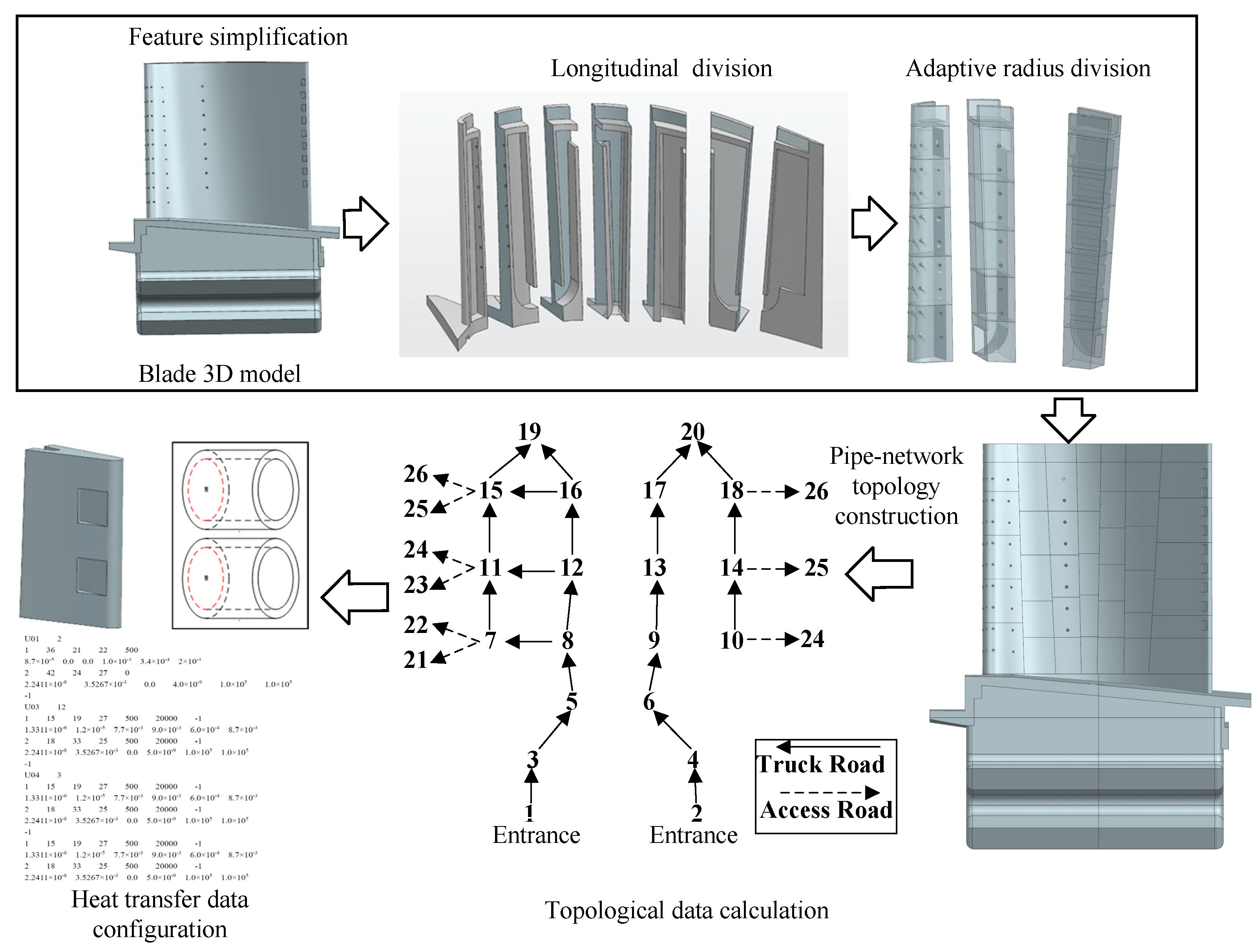
The traditional flow unit division based on manual operation has low efficiency and inconsistent standards, which cannot meet the requirements of automatic data extraction and data iteration. Therefore, an adaptive flow unit division method is presented, which is based on the skeleton lines of the pipe-network. The division plane of the longitudinal flow channel can be identified with the help of the skeleton lines. Then, according to the vertical flow channel obtained by cutting and the standardized input parameters, the boundary plane of the cooling structure is constructed. Finally, according to the marked division plane of the blade model, the flow units are divided adaptively.

3.2.1. Longitudinal Flow Channel Division Based on Skeleton Lines

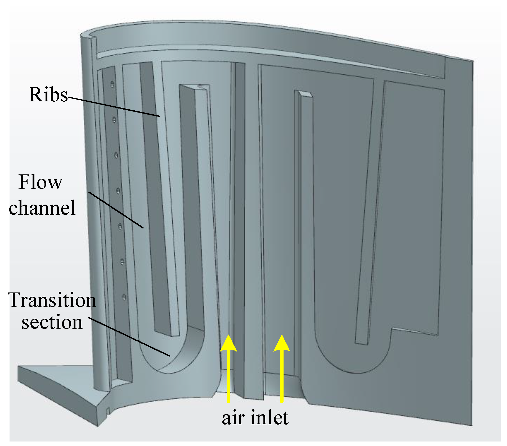
The flow channel of the turbine blade is mainly divided by the spacer ribs to form a plurality of flow cavities. Each flow cavity is connected by a transition section. Therefore, the spacer rib is an important reference for the longitudinal flow channel division of the turbine blade. The division reference planes are formed using the middle surface of the spacer rib and the two sides of the existing spacer rib. For better procedural expression, it is necessary to analyze the characteristics of spacer ribs. Turbine blade spacer ribs are illustrated in Figure 9.

(1) Geometric characteristics.

Generally, the rib’s side faces are geometrically ruled surfaces. They appear in pairs, although the paired side faces are not necessarily parallel.

(2) Location characteristics.

The transition section connects the side faces of the rib and is the starting point or end point of the flow channel and turning. Therefore, one of the side faces of the rib must be the interval between two adjacent flow paths or the turning position of a single flow path.

The skeleton line is an abstract expression of the three-dimensional fluid flow path. Therefore, the skeleton lines of the flow channels of the turbine blade are used to help to identify the position of the longitudinal division datum planes automatically. The basic idea of generating the longitudinal division planes is as follows. Firstly, the detail features such as spoiler ribs and air film holes on the blade are suppressed, because the detail features interfere with the extraction of the skeleton line and affect the extraction of the reference surfaces of the ribs. Then, all the surfaces of the blade are cycled and stored. All the side faces of the bending and torsion spacer ribs are identified and paired according to the two characteristics. Finally, the middle surface of the spacer rib is generated using the paired side faces, which are the longitudinal split surface. Hence, the longitudinal flow channel division steps based on the skeleton line are as follows.

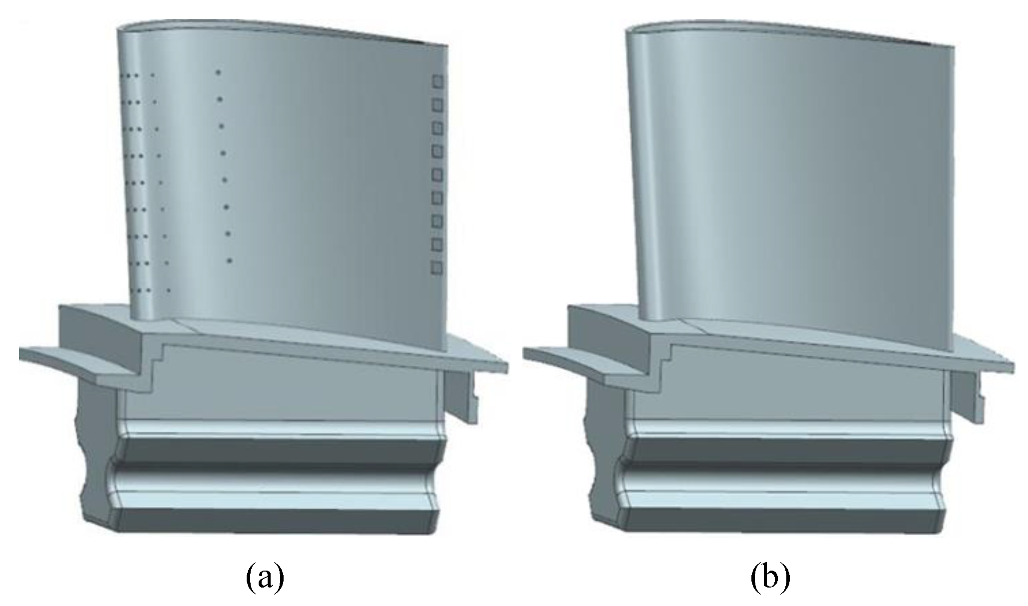
Step 1. Solid geometry model preprocessing—feature suppression.

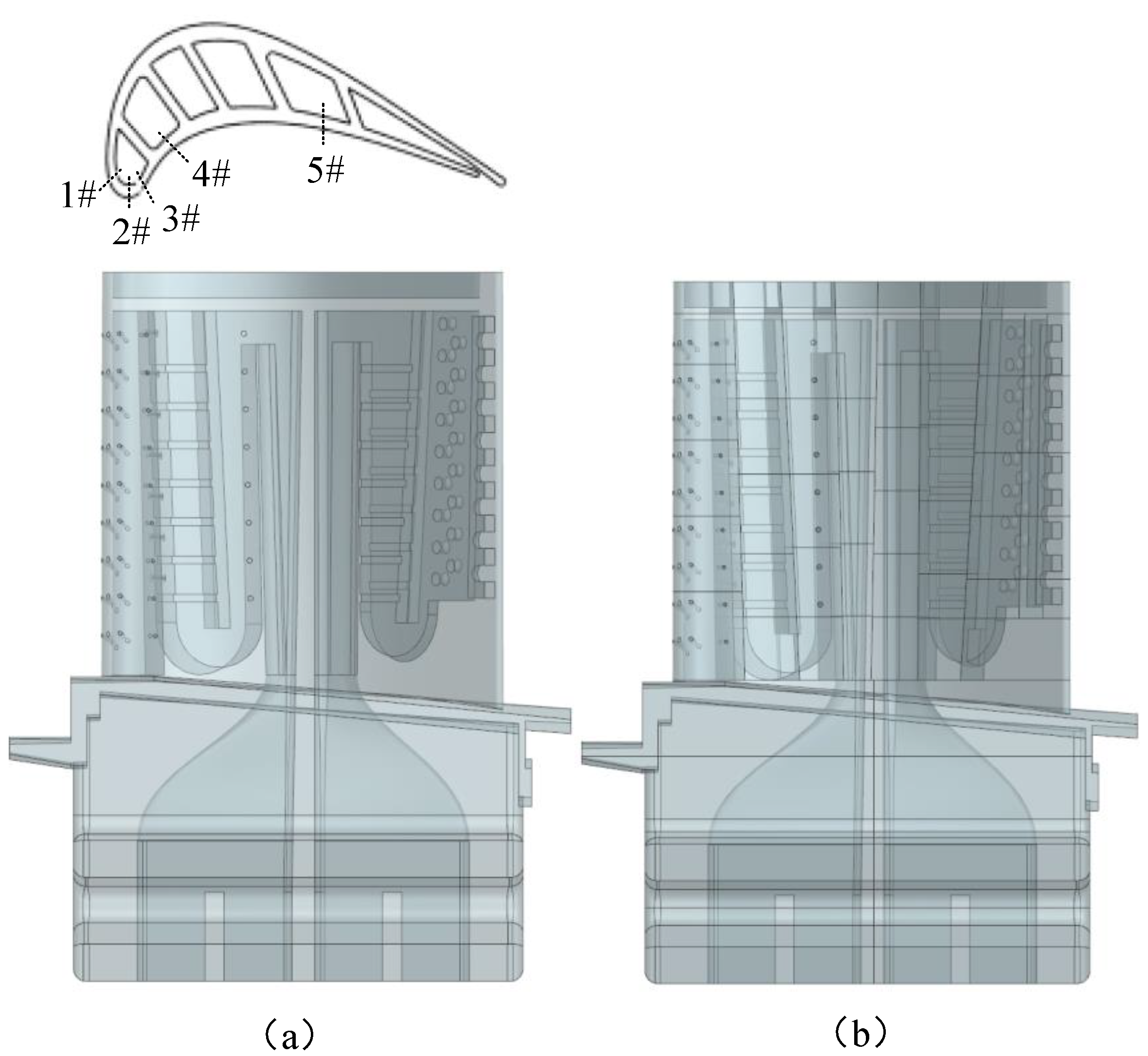
The blade geometric model $M_b$ is cycled to obtain the detailed feature set, such as air film holes, impact holes, tail seams, etc. The detailed features are suppressed. Figure 10 shows the blade models before and after detail features suppression.

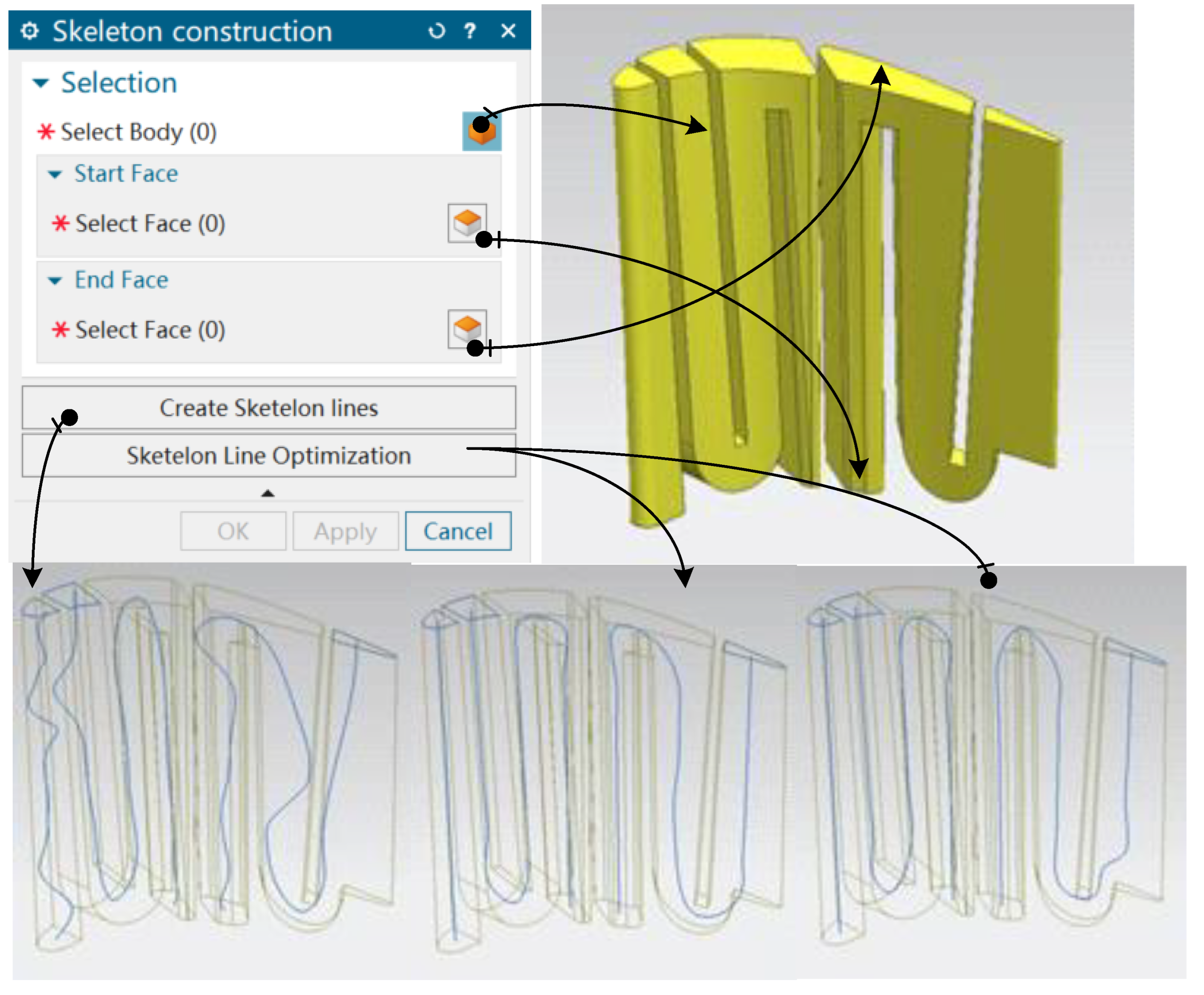
Step 2. Extraction and division of skeleton lines

The flow channel’s skeleton lines $\left\{{L_s}^i\right\}$ are generated using the method described in Section 2. Each skeleton line of every flow channel is divided into discrete points $\left\{{P_d}^i(x,y,z)\right\}$. The sequence of skeleton lines is obtained by sorting each starting point’s x coordinate of each skeleton line.

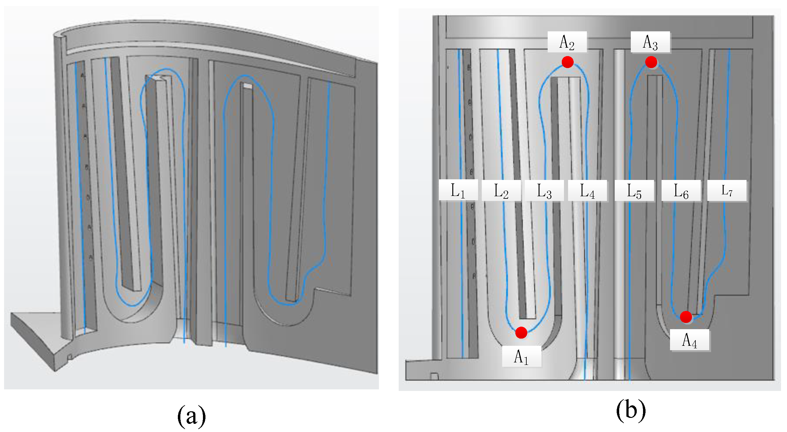
Step 3. Adaptive division of skeleton lines

The turning of the skeleton line depends on the transition section, which is adapted to the spacer ribs. Taking the radial z direction of blade model $M_b$ as the reference direction, the points in $\left\{P_d^i(x,y,z)\right\}$, which are the discrete points of each skeleton line, with maximum or minimum z value are calculated. To exclude possible error interference in skeleton line extraction, it is necessary to set the minimum radial spacing tolerance $\delta \left(z\right)$ of adjacent extreme points as a reference, exclude the extreme point between the tolerances $\delta \left(z\right)$, and store the extreme point with the larger radial z value, which is the appropriate turning point $\left\{A_n\right\}$ after the tolerance judgment. As shown in the Figure 11, at the four extreme points of $A_1$∼$A_4$, the initial skeleton line $L_s$ is divided into seven segments. According to the abscissa of the starting point of the blade spanwise coordinate, the adaptive segmented skeleton lines are recorded as $L_1\sim L_7$.

Step 4. Division faces filtering

All the face elements $\left\{Fac{e}_i\right|face\_type,\overrightarrow{n}\}$ of the blade model $M_b$ are cycled. All the face types and normal vectors are stored as the criterion. The criteria of judgment: (1) type filtering, $face\_type\ne datum\_plane$, design reference planes are excluded; and (2) direction judgment, $\overrightarrow{n}\ne 0,\pm 1$, the bottom faces of the spacer rib are excluded. An initial face set $\left\{Fac{e}_i\right\}$ can be obtained.

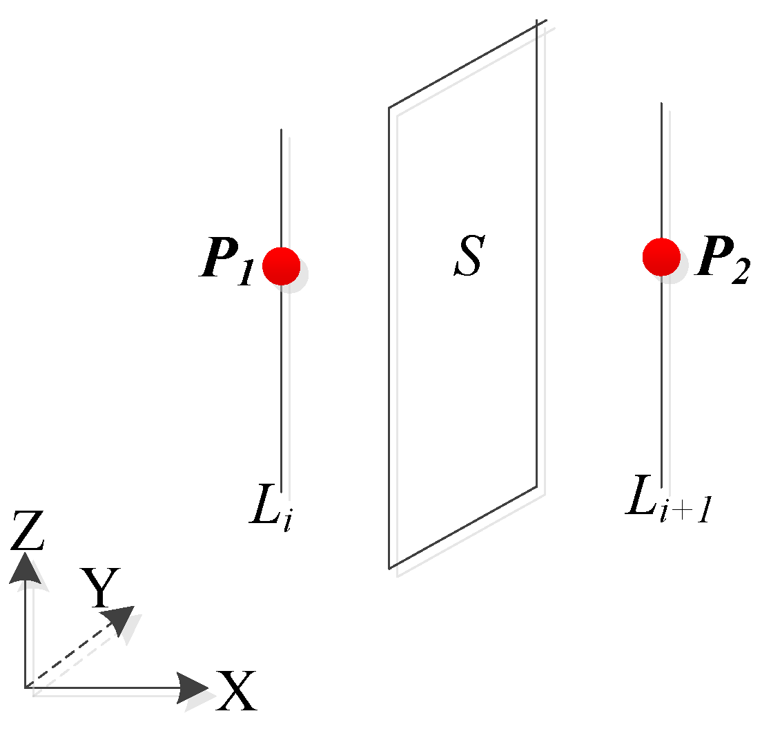
Step 5. Judgment of the relative position of the flow channel wall

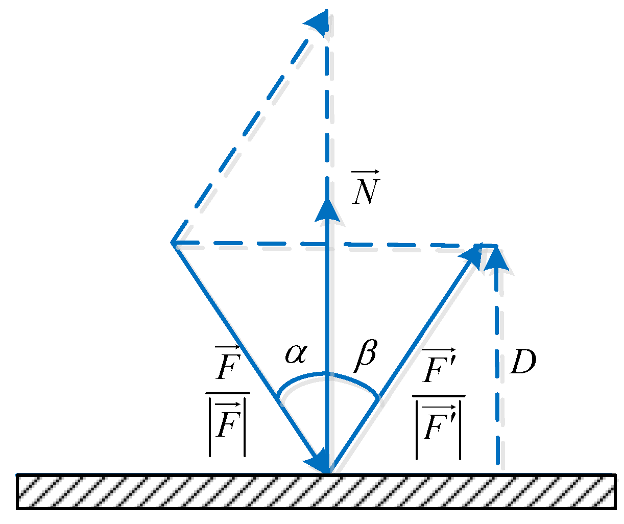
If $Fac{e}_j$ in $\left\{Fac{e}_i\right\}$ is the wall of the flow channel, then there is $m\in (0,7)$. When $i\le m$, the points on the skeleton line $L_i$ are all on the left side of the $Fac{e}_j$, and when $i>m$, the points on $L_i$ are on the right side of $Fac{e}_j$. Due to the existence of errors and the complexity of discreteness, the efficiency will be affected and the robustness will be poor if all discrete points participate in the above judgment. Therefore, two trisection points are selected for each skeleton line as reference points for judging the skeleton line according to the minimum point judgment criterion, as shown in Figure 12.

Judging the relationship between point and face: If the face $S:f\left(P\right)=0$ is the flow channel wall face, the points $P_1(x_1,y_1,z_1)$ and $P_2(x_1,y_1,z_1)$ are on the divided skeleton line, and $x_1<x_2$ is satisfied. Equation (2) must be satisfied.

$$f\left(P_1\right)<0,f\left(P_2\right)>0$$

(2)

All the flow channel walls faces $\left\{Fac{e}_i\right\}$, which are screened out in step 4, are cycled. For $\exists Fac{e}_j,\forall P_S=(x_s,y_s,z_s)\in Fac{e}_j$ and normal vetcor $\overrightarrow{n}=(a_s,b_s,c_s)$ of a plane ($a_s>0$), the following Formula (3) can be obtained.

$$S:f(x,y,z)=a_s(x-x_s)+b_s(y-y_s)+c_s(z-z_s)=0$$

(3)

Substitute Equation (2) into Equation (3). If the face is a flow channel wall face, then $\exists m\in (0,7)$, the reference point $p_i$ satisfies Equation (4).

$$\left\{\begin{array}{c}{a}_s(x_i-x_s)+b_s(y_i-y_s)+c_s(z_i-z_s)<0,i\le 2\ast m\hfill \\ a_s(x_i-x_s)+b_s(y_i-y_s)+c_s(z_i-z_s)>0,i>2\ast m\hfill \end{array}\right.$$

(4)

Finally, all the flow channel wall faces are found. They are classified and saved according to the value of m.

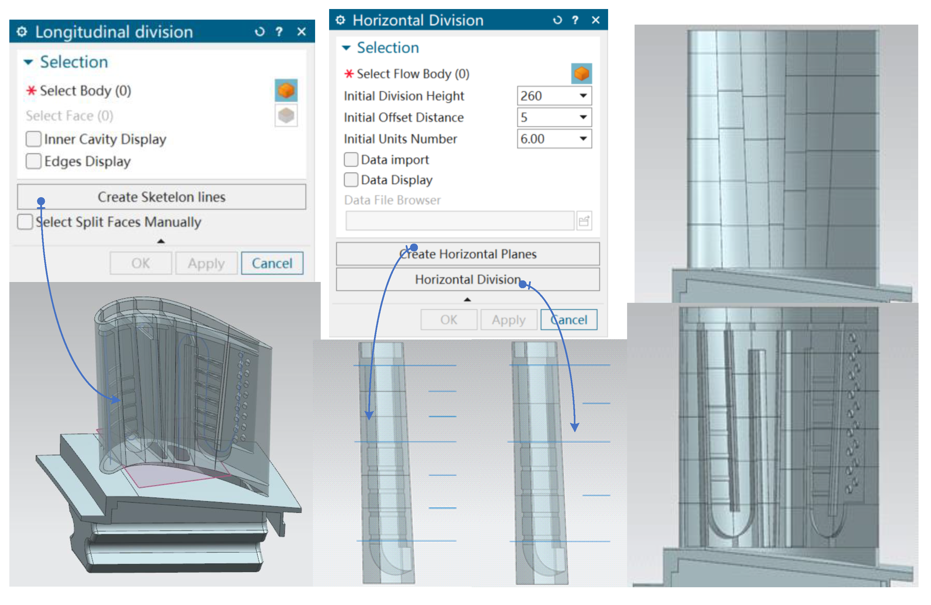
Step 6. Adaptive division

To further ensure the robustness of the algorithm and prevent the interference of some non-flow channel wall faces, the flow channel wall faces are screened and paired. For paired faces with more than 2 elements, they will be paired again under the consideration of the normal direction of faces. Then, the longitudinal split faces of the turbine blade are generated by creating the mid-face of the paired face.

According to the above algorithm, the blade model is divided into longitudinal fluid units adapted to the skeleton line of the flow channel, as shown in Figure 13.

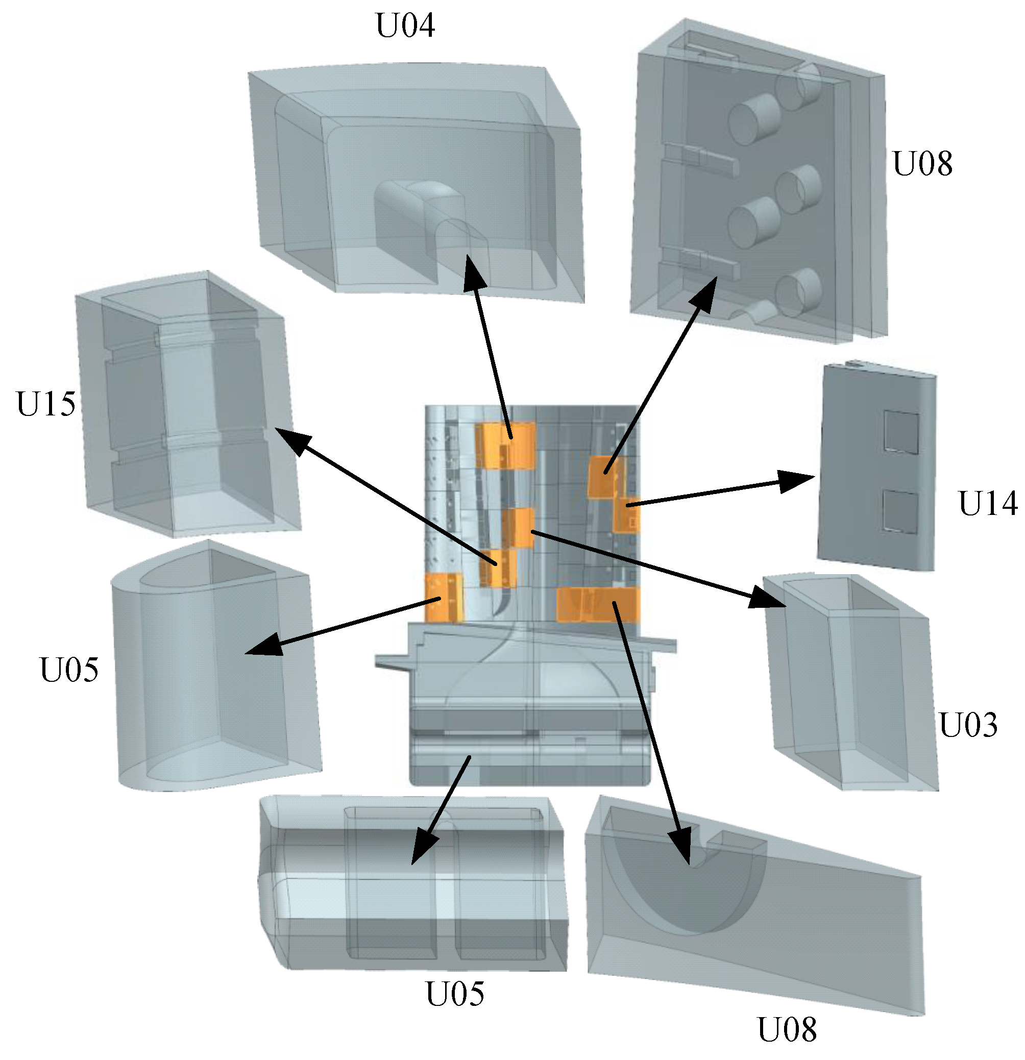
3.2.2. Feature Recognition of Flow Unit

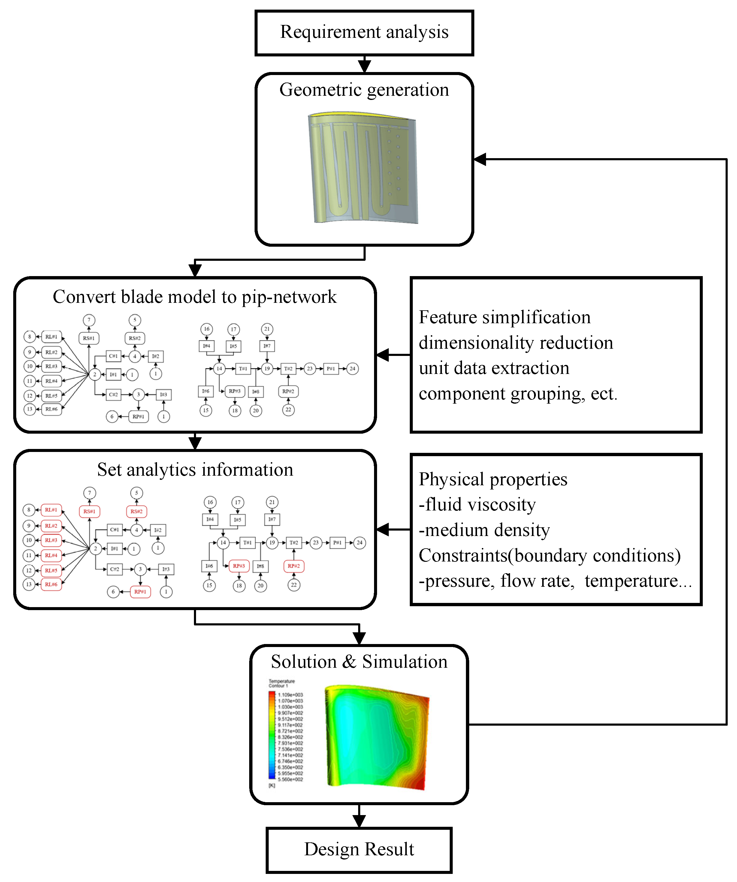
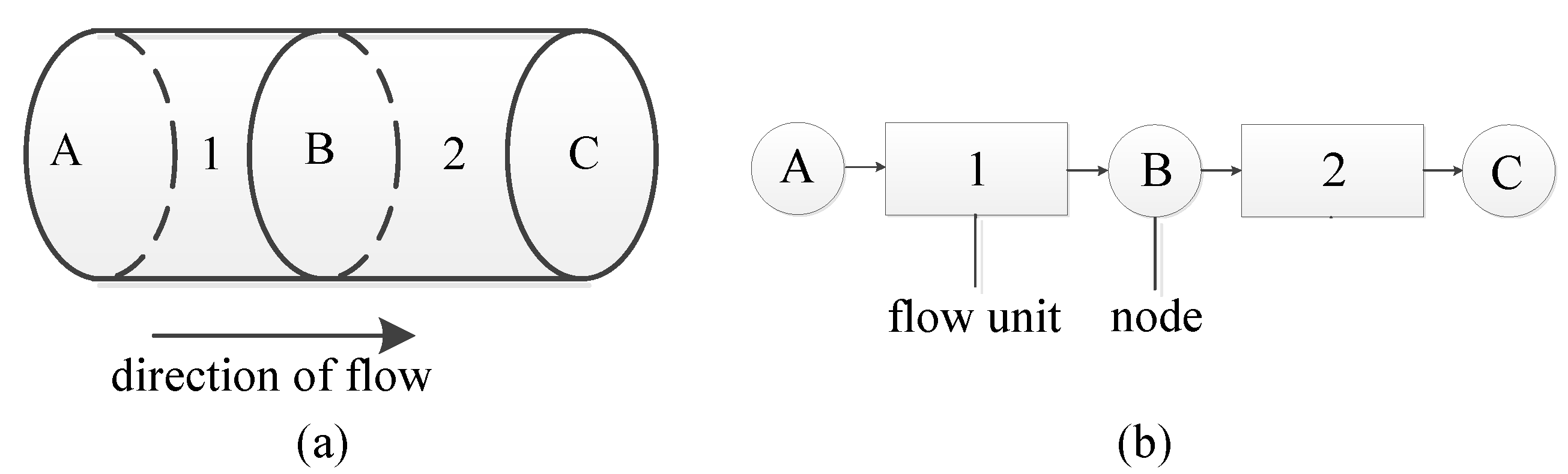
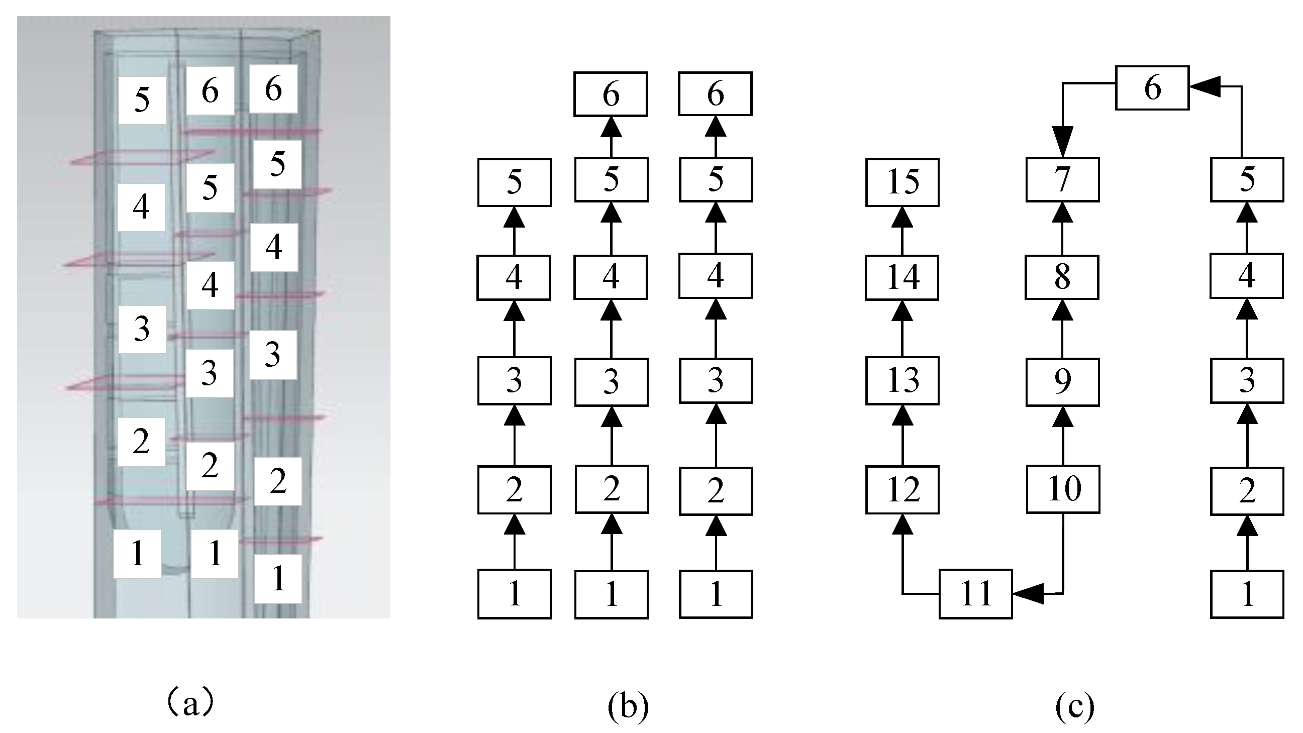
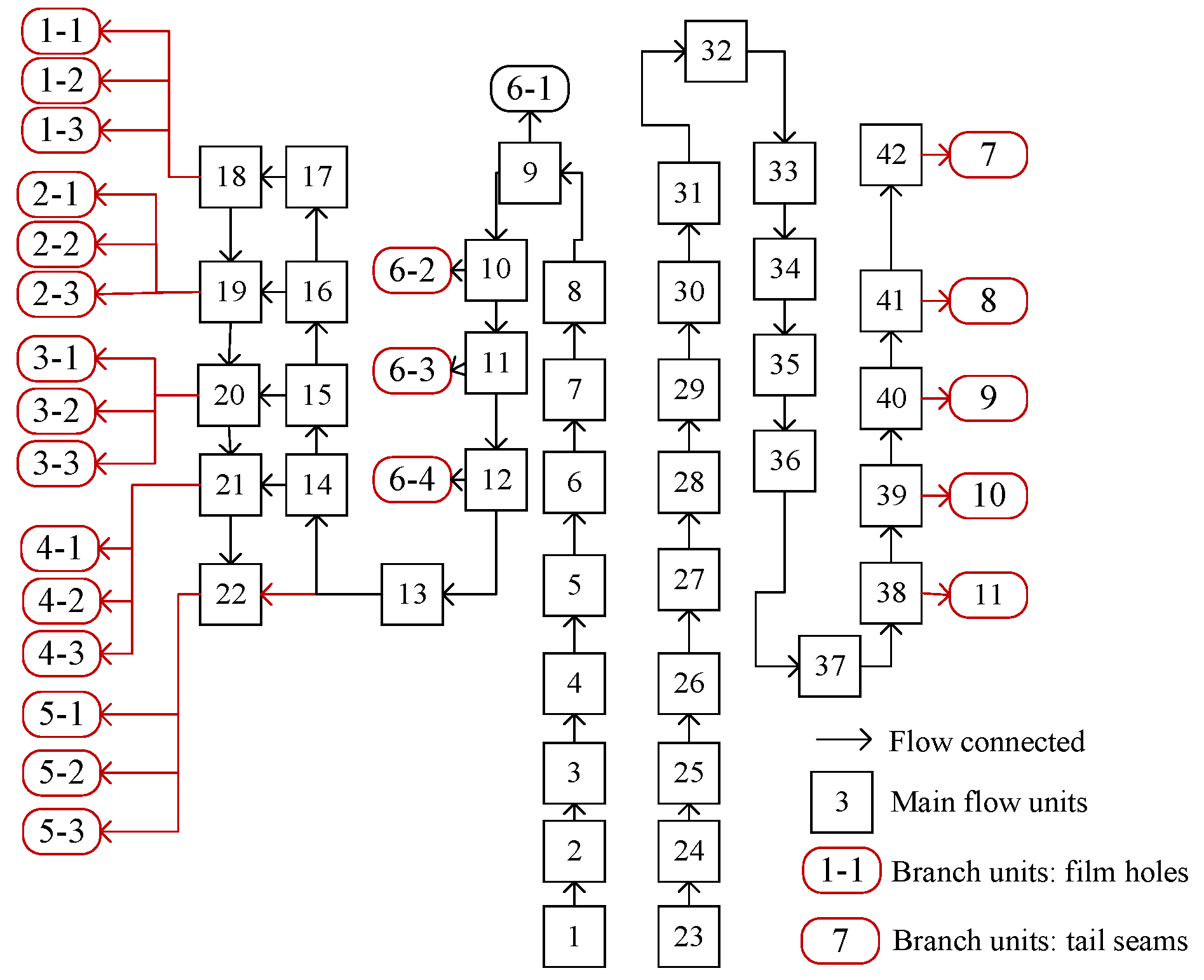
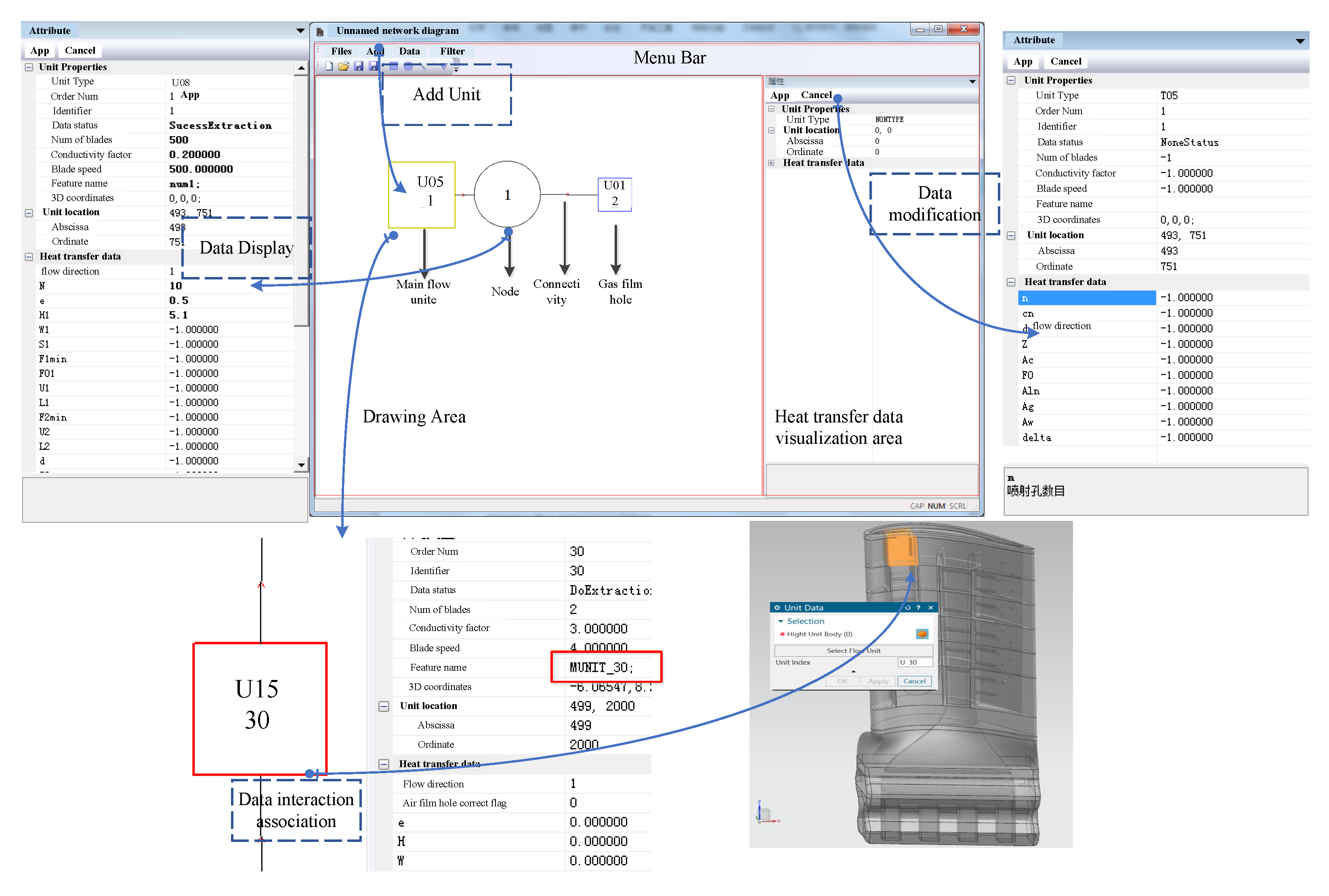
For each longitudinally divided flow channel, it can be abstracted into units that can be calculated one by one. The basic calculation logic principle is shown in Figure 14. Therefore, it is necessary to build a logical feature library of typical flowing units to facilitate feature recognition, data extraction, and data configuration. The logical features of flowing units are constructed and classified according to their heat transfer characteristics, as shown in

Table 1. Feature library of flowing units.

Name	Coding	Characteristic	Basic Model
Film cooling unit	U01	Orifice without considering flow loss
Smooth straight pipe unit	U03	Heat transfer functions, smooth rectangular tubes regardless of local losses
$\pi$-shaped bending unit	U04	Rotation and heat transfer functions, 180° $\pi$-shaped elbow, rectangular section.
Impact cooling unit	U05	Heat exchange unit of single row circular jet impinging on semicircular concave surface
Spoiler unit	U08	Rectangular channel with the combined influence of transverse rib and spoiler column
Circular elbow unit	U09	180° circular elbow with rotation and heat exchange, rectangular section
Tail seam unit	U14	Heat exchange
Flow channel unit with spoiler ribs	U15	Rectangular channel with two opposite side walls with spoiler ribs with a certain included angle

, which covers most flowing structures of turbine air-cooled blades.

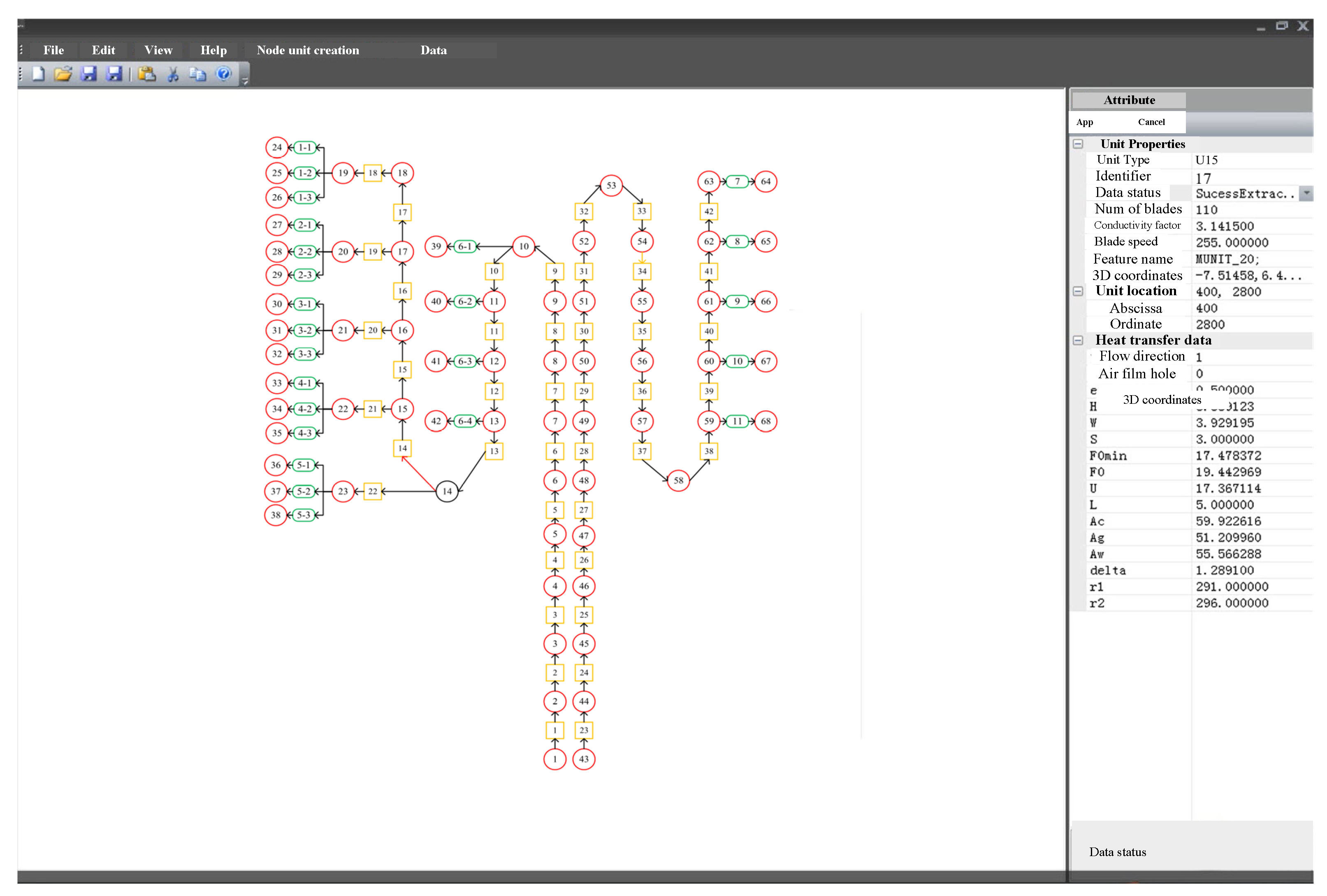
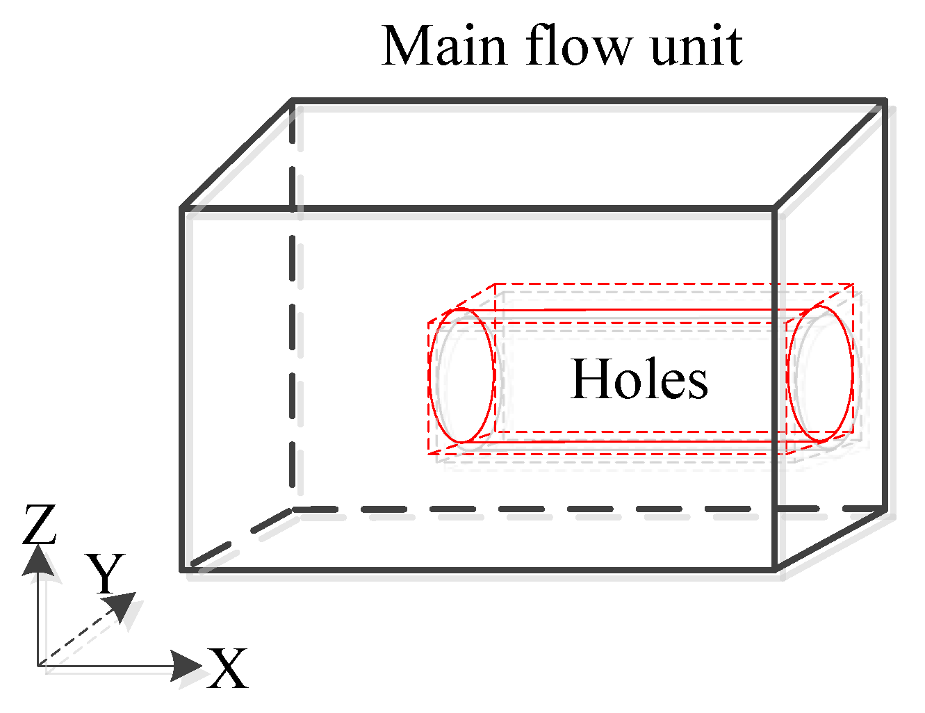
According to the position of the flowing units in the flow channel, it can be divided into two categories: main flowing unit and additional structural unit. The typical flowing units are shown in Table 1. The main operations of the main flow unit are as follows: flow unit determination, parameter extraction, and unit calculations. The basic calculation process of main flowing units is shown in Figure 15. The additional structural unit is calculated after the main flow unit calculation. Because they include detailed features such as air film holes, tail seams, impact holes, etc, the detailed features are feature-suppressed during the adaptive division of the flowing channels.

The main channel unit is characterized in turn according to the order of the elbow unit and the straight channel unit.

(1) Feature recognition of elbow unit

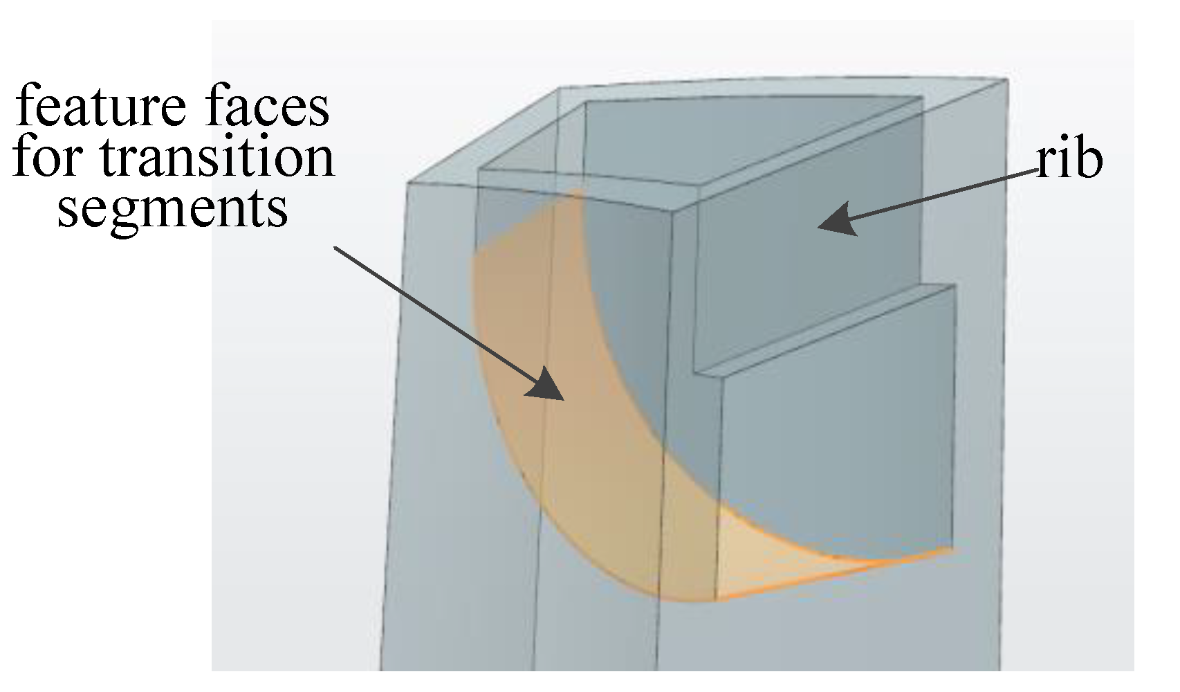
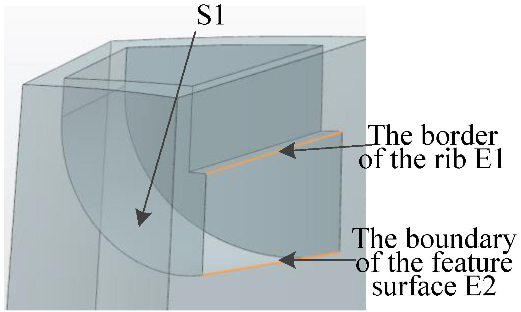
Such flow unit features are mainly distributed at the turn of the flow channel, which can be divided into $\pi$-shaped elbow units and circular elbow units. The main features identified are position and structure. In terms of position recognition, the position distribution can be judged according to the turning pole of the skeleton line. In the previous section, the extreme point of the skeleton line was calculated and discriminated, so the division points of the skeleton line can be selected as the layout feature points of the elbow unit feature. If the structure is completely recognized and extracted, it is necessary to ensure the integrity of the internal cooling structure: (1) feature surface of the transition section, and (2) part of the wall of the partition rib. As shown in Figure 16, these two features contain heat transfer data such as turning radius, inlet/outlet section width, etc.

Hence, the recognition Algorithm 2 of elbow unit features is as follows.

Algorithm 2:

Step 1. The face set of the longitudinal segments is cycled to find the wall faces generated by the longitudinal segments. The distance between the planes parallel to the longitudinal cut surface and the marker point are calculated. The face with the smallest distance is the wall face. The curve set of the wall face is cycled. The curve set is connected into rings according to the topological relationship. The minimum ring where the marker point is located in the boundary ring of the elbow unit feature containing key data. Step 2. All elbow units are found according to the location characteristics. The  curve elements in the elbow units are cycled and queried according to the Z-direction average value of the curve elements. The curves with maximum and minimum Z-direction average value entrance are the characteristic edge E1 and the characteristic edge E2 to be identified, as shown in Figure 17.

The faces of the longitudinally divided unit are cycled to find the elbow feature face S1, one of whose edges is connected to E1. S1 is set as the elbow unit feature classification surface, which is used to identify and classify the type of elbow units. The main judgment criteria are the characteristic surface type. (1) If the surface’s type is a plane, the unit is denoted as U04, a feature of the $\pi$-shaped elbow unit. (2) If it is not a plane, it is a U09 unit, a feature of a circular elbow unit.

(2) Feature recognition of straight flow channel units

After the elbow units in the longitudinally divided unit are recognized, the rest of the units are composed of straight-flow channel units. The straight units include a smooth straight pipe unit U03, an impact cooling unit U05, a unit with a spoiler column U08 and a unit with a rough spoiler rib U15. The classification of these types of units is based on features such as spoiler columns and spoiler ribs. Therefore, the key to this step lies in the recognition of two types of cooling features. The recognition steps are: All face elements of the blade model are cycled. The faces of the Z-direction bounding box within the Z-direction bounding box of the skeleton line are stored. In the face set, according to the characteristics of each cooling feature, the spoiler column and spoiler rib are recognized in turn. The two types of cooling features are recognized as follows.

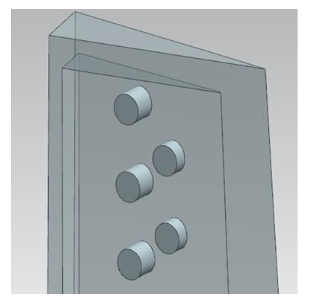
Spoiler column: The spoiler column is usually designed at the trailing edge of the airfoil cavity, as shown in Figure 18. The section is mainly circular, and its characteristic surface is cylindrical. The cylinder surface in the solid has fillets in addition to the spoiler column. However, the coverage of the fillets is a sector area, while the spoiler column is a complete circle and the number of boundaries of the two is different. Therefore, all the faces are cycled in the face set to find the faces whose type is cylinder $(fac{e}_{type}=cylinder)$. The edge elements associated with the cylinder are obtained. The face with two edges is the spoiler column. The Z average value of each spoiler column bounding box is recorded. It is arranged in the array $spoiler$ in ascending order.

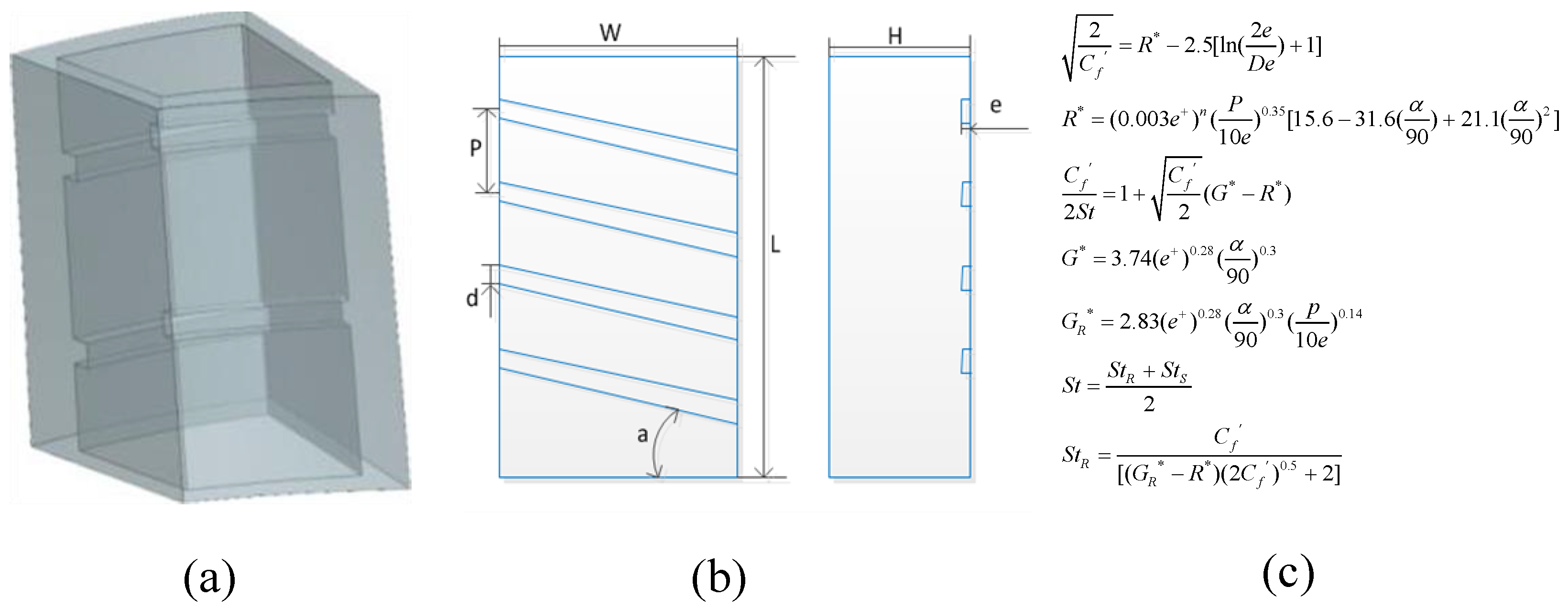
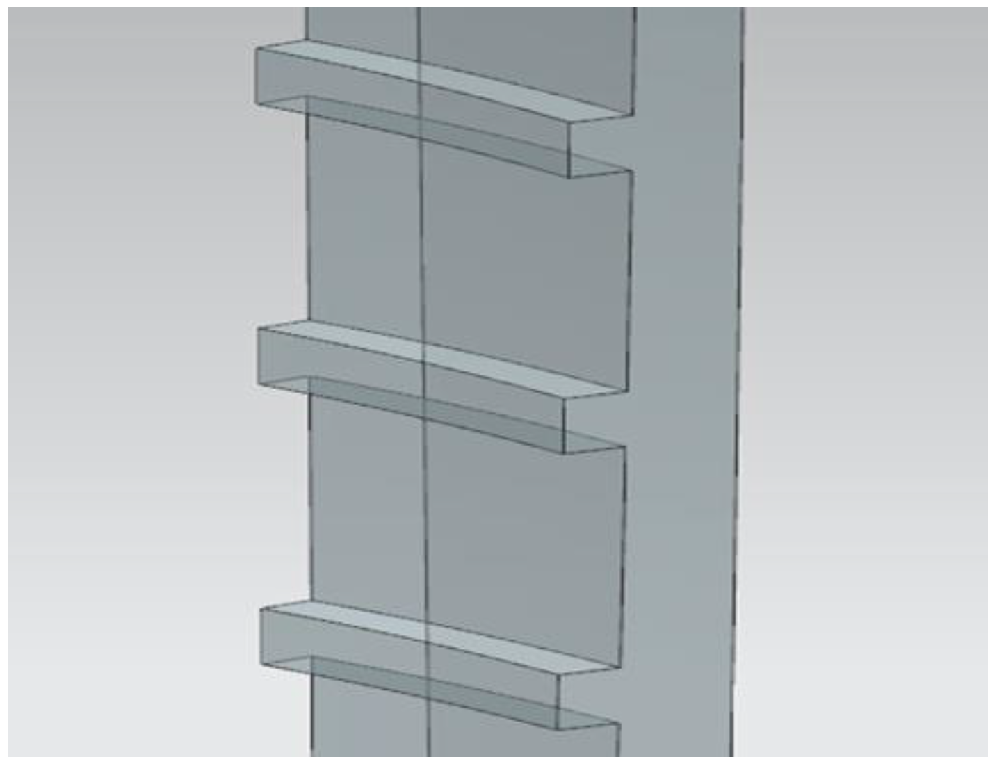
Spoiler rib: The spoiler ribs usually exist in the form of an array on the back of the blade or the blade basin. The top and bottom surfaces of each spoiler rib are a set of planes that are parallel to each other and are parallel to the top and bottom surfaces of other spoiler ribs on the same row, as shown in Figure 19. Therefore, the planes in the face set can be grouped by the normal direction, and the number of group elements that is more than 4 is the spoiler rib surface. Since the directions of each row of spoiler ribs are not necessarily the same, there may be multiple groups of spoiler rib planes obtained. We record the Z mean value of each plane and arrange it in the array rib in ascending order.

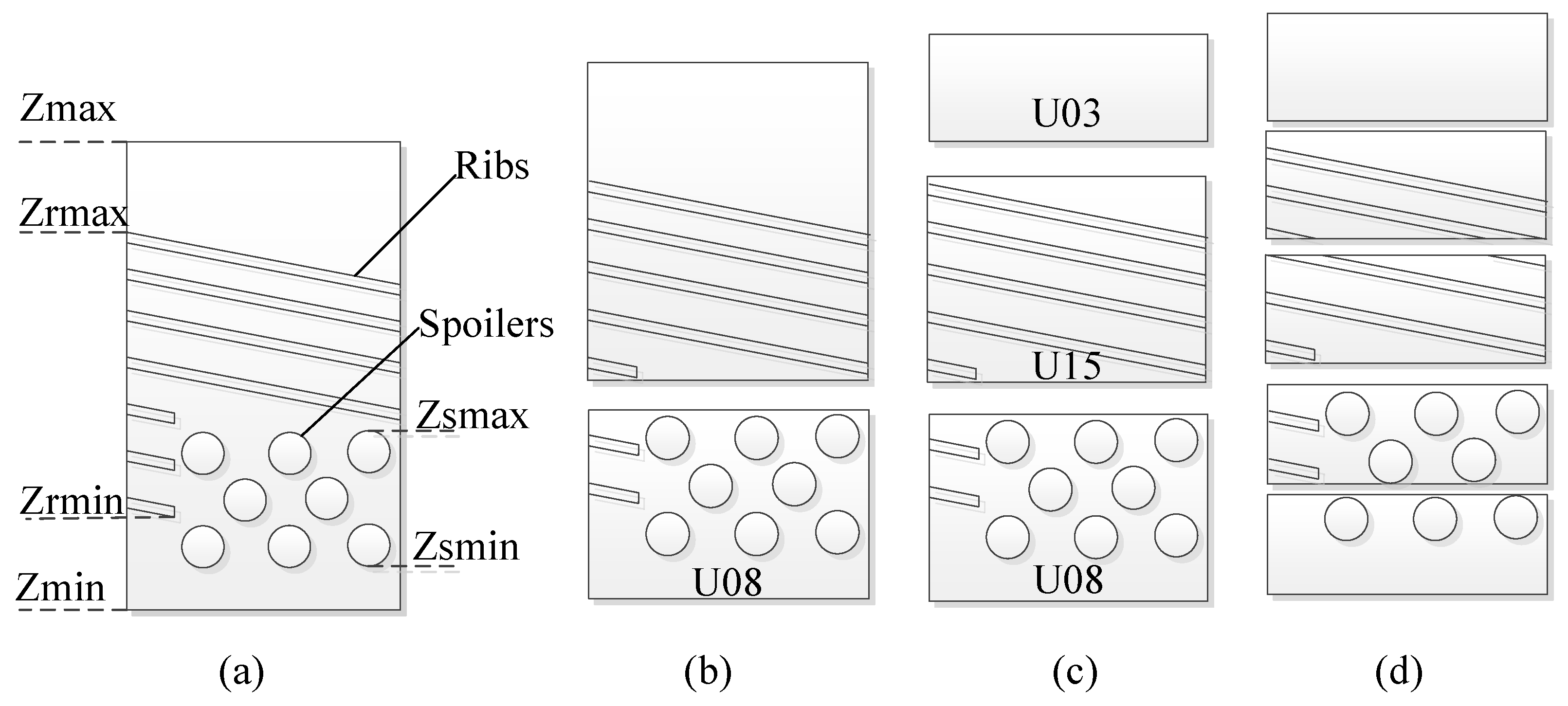
The longitudinal unit that does not contain spoiler ribs and spoiler columns is a smooth straight pipe unit or an impingement cooling unit. Next, it is necessary to generate the diameter division faces according to the position information of the spoiler columns and the spoiler ribs. In the process, a unit height H needs to be set to ensure that the height of each unit is in a suitable range. The diameter division faces generated method is as follows. Firstly, the spoiler column array $spoiler$ and the spoiler rib array $rib$ are traversed, whether there are elements whose adjacent coordinate value spacing is greater than H. If it exists, it means that there are other types of straight flow units between them. The array is divided again based on this. Since spoiler ribs are allowed to be included in the unit with spoiler column $U08$, the divided face for each group of spoiler columns according to the Z-coordinate range is $Z_{smin}$∼$Z_{smax}$ of each group of spoiler columns. It is necessary to judge whether the distance between $Z_{smin}$ and the boundary $Z_{min}$ of the whole longitudinal partition block is greater than the reference value H of unit height. If so, a divided face is generated in $Z_{smin}$, otherwise the part between $Z_{smin}$ and $Z_{min}$ will be incorporated into the spoiler column unit. After the spoiler column unit is divided, the interface between the spoiler rib and the smooth straight pipe unit is planned in the same way. After all the interface settings are completed, the flow unit is divided in sequence from the bottom to the top. The flow of the scheme is shown in Figure 20.

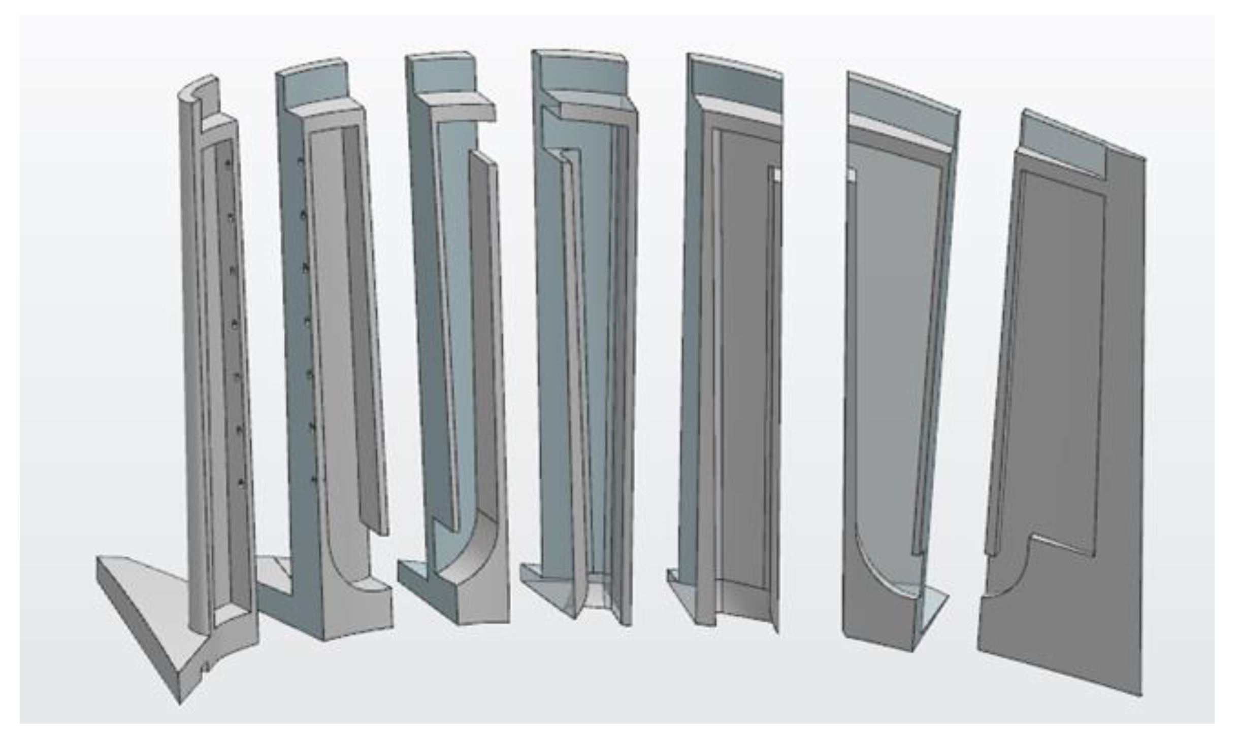
Based on the above diameter steps, in the order from left to right, the cooling structure is recognized and divided for each longitudinal flow channel in turn. A blade model adaptive division result is shown in Figure 21.

4. Pipe-Network Topology Construction

4.1. Judgment of Flow Units Connection Relationship

(1) Main flow channel units connection relationship judgment

According to the typical units library and skeleton line, the type judgment and feature recognition of the flow units are carried out. According to the auxiliary skeleton line, the divided flow units are arranged in sequence. The units connectivity can be judged according to the skeleton line and the serial number, as shown in Figure 22. Due to the separation of the flow channels, the parallel single-row flow channels need to be merged. The criterion is based on the connection relationship of the skeleton line and whether the elbow unit is included. Finally, the connection relationship of the complete main flow channel is constructed, as shown in Figure 22c.

(2) Branch channel units connection relationship judgment

Some detailed features, such as film holes, tail seams, etc., are the branch channel units. The judgment of the relationship between the main channel units and the branch channel units is based on minimum bounding box collision detection [34]. Figure 23 is a schematic diagram. The collision detection is carried out with the minimum bounding box of the main flow unit. The collision detection conditions are met, and the two units have a connected relationship. In addition, if a branch flow unit and multiple mainstream units meet the collision detection conditions, the connectivity relationship needs to be determined according to the collision depth and collision sequence. Generally, it will be regarded as the main connected relationship with the first main flow unit that it “collides” with, and the others can be ignored or left for further judgment.

4.2. Pipe-Network Topological Model Construction of Blade Model

Based on the above connection relationship judgment method between main flow units and branch flow units. The topological connectivity of each component of the blade flowing channel is obtained as shown in Figure 24. Two mortise inlet units are designated as inlet units. The fluid network topology model of the flow channel of the air-cooled blade can be obtained, as shown in Figure 25.

5. Flow Units Data Extraction for Pipe-Network Calculation

5.1. Flow Units Data Analysis and Classification

In the pipe-network calculation system, different flow units require different flow and heat property parameters, but the parameters have a certain commonness. These parameters are used to describe the overall, inlet, details, heat transfer, and rotation status of the flow channel. The geometric structure of $T15$ unit and the corresponding flow heat element model are shown in Figure 26. When abstracting this unit, it is necessary to configure multiple parameters such as rectangular channel data, rib parameters, and fluid physical properties for the calculation of key data such as pressure drop, flow resistance, and the heat transfer coefficient.

Table 2. Some important data of $U15$ unit for pipe-network calculation.

Parameters	Parameter Description	Parameters	Parameter Description
e	Rib height	$Ac$	Internal heat exchange area
$\alpha$	Rib angle	$Ag$	External heat exchange area
S	Rib distance	$Aw$	Heat conductivity area
b	Rib width	L	Length of flow channel
H	Height between two ribs	$r_1$	minimum Z of the unit
W	Flow channel width	$r_2$	maximum Z of the unit
$F0$	Inlet flow area	n	Blade number
U	Inlet wetted perimeter	$\lambda$	Heat conductivity coefficient
$F{0}_{min}$	Minimum flow area	$\omega$	Rotating speed
$\gamma$	Wall thickness of flow channel

shows some important data required by the rib element in a pipe-network calculation model under the consideration of rotating heat transfer. From the perspective of data extraction, the relevant data can be divided into the following categories.

(1) Parameters, which are geometric structure modeling parameters. For example, the rib height, rib spacing, and other parameters in Table 2. These parameters are just the control parameters of the geometric modeling of the spoiler rib. The relevant design parameters explicitly exist in the CAD model, which can be easily accessed through the relevant modeling conventions and specifications.

(2) Geometric property parameters of the flow unit, such as the rectangular channel parameters and heat transfer area-related parameters in the $T15$ unit in Table 2. These parameters can only be obtained by geometric measurement and analysis-oriented conversion calculation since these parameters cannot exist explicitly in the geometric model.

(3) Physical parameters unrelated to geometry, such as thermal conductivity of blade material, blade speed, etc. These parameters are generally given based on working conditions, and all components abstracted from the same blade can be used universally.

From the perspective of extraction, this paper only needs to focus on the measurement and extraction of geometric structure-related parameters. These geometric structure-related data parameters can be divided into length, area, radius, and angle types. Based on the geometric and functional meanings of physical attribute parameters, the analysis parameters are classified in this paper, and the results are shown in Figure 27.

5.2. Flow Unit Data Extraction for Pipe-Network Calculation Based on Function-Geometry Mapping

The extraction data related to the geometric structure of each flow unit of the blade should follow the steps of (1) functional domain decomposition, and (2) data redefinition and analysis feature recognition. The following introduces the extraction method of data extraction of the flow unit, taking the geometric unit with the spoiler rib shown in Figure 26 as an example.

(1) Functional domain division of air-cooled blades

Based on the analysis principle of pipe-network calculation and the classification and definition of analysis parameters, the functional domain of the air-cooled blade is analyzed. The functional domain can be divided into the hot gas domain (extract the relevant temperature parameters such as the heat exchange area on the gas side), the cold air domain (calculate the parameters such as the cold air pressure and flow rate), and the combination domain of the two. The geometric structure corresponding to each sub-functional domain has obvious boundaries, so the blade geometric unit can be decomposed into geometric domains based on the functional domain decomposition. Each analysis parameter can be mapped to each sub-geometric domain. The domain decomposition logic of the main components/units of the air-cooled blade air system is shown in Figure 28.

For the blade element with spoiler rib $U15$, according to the above domain decomposition logic, it can be divided into the cold air domain, the gas domain, and the combined domain. An adjacency diagram is constructed for the unit $U15$, from which the nodes at the inlet and outlet surfaces of the flow cavity are identified, that is, the adjacency diagram of the element is automatically divided into subgraphs representing the gas domain surface ring, and the cold gas domain flow cavity surface ring, respectively, using the subgraph decomposition method. After domain decomposition of this type of unit, the color is used to represent the face elements contained in each sub-geometric domain. The results are shown in Figure 29, in which a large number of fillet features are suppressed for the convenience of display. At the same time, since the blade longitudinal rib is assumed to be adiabatic in the pipe-networks calculation, the geometric elements of the cold air region and the gas region can be logically further divided into heat exchange surface set and thermal insulation surface set for later description.

(2) Physical parameters redefinition and corresponding analysis feature recognition

The parameter redefinition is carried out on the premise of the decomposition of the cold and hot gas domains. The parameters are redefined using geometric elements in each sub-geometric domain. In this process, the most important thing is to ensure the applicability of the analysis parameters in the same element type, but with different geometric structure elements. As for the $U15$ unit, if many fillets in the flow cavity are retained or the number of spoiler ribs in the flow cavity changes, the geometric topology composition of the cooling geometric domain is greatly different. Therefore, when redefining parameters, geometric elements should be used to avoid large topological changes. For similar reasons, the same criteria should be followed in the subsequent analysis of feature definition and recognition rule design. Regarding this criterion, the geometric redefinition of geometric-related physical attribute parameters in ribbed elements is listed in

Table 3. Analysis parameters redefinition.

Parameters	Redefinition	Redefinition Description
H	$H=Dis([P_{mid}^b,e_b^c],[P_{mid}^p,e_p^c])$	Distance between inlet concave edge $e_p^c$ mid-point $P_{mid}^p$ and convex edge $e_p^c$ mid-point $P_{mid}^b$
W	$W=Dis([P_{mid}^{n1},e_{n1}^c],[P_{mid}^{n2},e_{n2}^c])$	Distance between inlet edge $e_{n1}^c$ mid-point $P_{mid}^{n1}$ and edge $e_{n2}^c$ mid-point $P_{mid}^{n2}$
$F0$	$F0=Area\left(f_R\right)$	Area of face $f_R$ filled by the ring $R\{e_p^c,e_b^c,e_{n1}^c,e_{n2}^c\}$
U	$U=Length\left(R\right)$	Perimeter of the ring R
$F{0}_{min}$	$F{0}_{min}=F0-2e\ast W$	Inlet area minus area of opposite rib
$\gamma$	$\gamma =Aver\left(minD(e_{p/b}^c,S_{heat}^{gas})\right)$	Average of minimum distance between inlet edges $e_p^c$/$e_b^c$ and face set $S_{heat}^{gas}$
$Ac$	$Ac=Area\left(S_{heat}^{cool}\right)$	Area of face set $S_{heat}^{cool}$
$Ag$	$Ac=Area\left(S_{heat}^{gas}\right)$	Area of face set $S_{heat}^{gas}$
$r_1$	$r_1=Z_{min}\left(Bounding\left(S\right)\right)$	Minimum Z of the unit body bounding box
$r_2$	$r_2=Z_{max}\left(Bounding\left(S\right)\right)$	Maximum Z of the unit body bounding box

. The geometric elements involved in the parameter definition are summarized as analysis features. See

Table 4. Analysis features definition and recognition rules.

Analysis Feature	Feature Definition&Recognition Rules
R	Ring with minimum perimeter in $f_i$
$e_{n1}^c/e_{n2}^c$	Edges with approximate curvature of 0
$e_p^c/e_b^c$	Edges in R besides $e_{n1}^c/e_{n2}^c$
$S_{nheat}^{cool}$	Surface containing $e_{n1}^c/e_{n2}^c$ in $S^{cool}$ face set
$S_{nheat}^{gas}$	Surface with curvature close to 0 in $S_{gas}$ face set
$S_{heat}^{gas}$	$S^{gas}-S_{nheat}^{gas}$
$S_{heat}^{cool}$	$S^{cool}-S_{nheat}^{cool}$

for the definition rules.

6. Software and Examples

6.1. Software

A software system has been developed for calculating data extraction and configuration of turbine blade pipe-network calculation. It mainly includes two modules, the bottom development environment module, and the functional module, as shown in Figure 30. Siemens NX is the geometric algorithm library, which is used as the blade CAD model reading, flow units adaptive segmentation, and flow unit data calculation. Visual Studio is the interface layer, which is used to draw the network diagram, and to configure the data of the flow unit. Figure 31 and Figure 32 show the automatic extraction, optimization, and adaptive segmentation interfaces of turbine blade flow path skeleton lines. Figure 33 shows the drawing of the pipe network diagram and node data configuration.

6.2. Examples

A dual-channel rotor blade with a complex cooling structure is designed, and its modeling and simulation process is introduced. First, the blade structure design is completed based on the blade parametric design system, including the blade body, tail seam, spacer rib, spoiler rib, spoiler column, root extension, tenon, flange plate, impact hole, air film hole, etc. The blade geometric model is shown in Figure 34a. The blade is quickly decomposed into geometric units with specific cooling characteristics by using an adaptive division method based on skeleton lines, as shown in Figure 34b. According to pipe-network requirements, each unit is abstracted as a component, the topological connectivity between the units is calculated, and the physical attribute data are extracted. By importing the above-extracted data into the network diagram platform, the data of elements, nodes, topological connectivity, and element attributes can be visualized for verification and correction by designers, as shown in Figure 35. The extracted data are stored in a user-defined format, as shown in Figure 36a. Finally, the analysis data file conforming to the input format of the pipe-network calculation system is exported from the network diagram platform, as shown in Figure 36b. It is directly input into the pipe-network calculation system, which can solve the key parameters of flow and heat at each element and node within a few seconds, and output them in a specific data format for designers to evaluate the rationality of the blade fluid design scheme, and provide necessary boundary data for subsequent temperature field calculation.

In this case, a new cooling scheme can be generated by modifying the air film hole diameter of the blade shown in Figure 34 and fine-tuning the angle of the rib. Among them, the gas film holes’ diameter is 0.35 mm in the original Scheme I, and the gas film holes’ diameter is modified to 0.55 mm in the newly generated Scheme II. The flow heat design results of the two schemes can be quickly obtained and compared using the presented data extraction method and pipe-network calculation system.

Table 5. Calculated cold air flow results of pipe-network calculation: (The unit is %. CAC, cold air consumption; GOFL, gas output of film hole; DH, dedusting hole).

Scheme	All CAC	Front Cavity CAC	Back Cavity CAC	1# GOFH	2#GOFH	3#GOFH	4#GOFH	5#GOFH	Tail Seam	Front Cavity DH	Back Cavity DH
I	3.191	1.505	1.686	0.188	0.204	0.203	0.512	0.175	1.424	0.233	0.262
II	3.492	1.806	1.686	0.244	0.253	0.254	0.615	0.227	1.424	0.213	0.262

shows the cold airflow at the inlet and outlet nodes of the two schemes. Figure 37 shows the medium temperature and nodes on a cold air flow path of the blade (left flow path shown in Figure 35). The flow and heat parameters obtained from the pipe-network calculation system are taken as part of the boundary of the temperature field calculation. It can be seen from the comparison of schemes that the cooling effect of Scheme II is better due to the larger pore diameter and larger cooling air consumption.

Using the method presented in this paper, the extraction of blade flow heat data is shortened from several working days to several minutes. The iteration time of blade geometric modeling and thermal analysis is shortened from more than one week to several hours, which effectively improves the design efficiency and reduces the workload of the designers.

7. Conclusions

This paper presents a method for blade model adaptive division and analysis data extraction of divided flow units aiming at promoting the efficiency quality of analysis data preparation for turbine blade pipe network calculation. The results of the cases verified the applicability and stability of the proposed method. The main conclusions are summarized as follows:

(1) A skeleton line extraction method based on the principle of imitation fluid flow is proposed, which can automatically generate and iteratively optimize the flow path skeleton line. By simulating the characteristics of airflow, this method realizes the self-adaptive division of flow units and the automatic judgment of the connectivity of flow units based on the skeleton line calculation without the assistance of manual interaction and the identification of complex geometric feature units.

(2) Through the functional topology data extraction algorithm of each unit, the automatic construction of the analysis data model and pipe network topology network diagram required for pipe network calculation of the blade is realized.

References

1. Han, J.C.; Sandip, D.; Srinath, E. Gas Turbine Heat Transfer and Cooling Technology; CRC Press: Boca Raton, FL, USA, 2012; pp. 5–14. [Google Scholar]
2. Yan, P.G.; Shi, L.; Wang, X.F.; Han, W.J. Retrofit design of composite cooling structure of a turbine blade by fluid networks and conjugate heat transfer methods. Sci. China Technol. Sci. 2013, 56, 3104–3114. [Google Scholar] [CrossRef]
3. Amaral, S.; Verstraete, T.; Van den Braembussche, R.; Arts, T. Design and optimization of the internal cooling channels of a high pressure turbine blade—Part I: Methodology. ASME J. Turbomach. 2010, 132, 021013. [Google Scholar] [CrossRef]
4. Nourin, F.N.; Amano, R.S. Review of gas turbine internal cooling improvement technology. ASME J. Energy Resour. Technol. 2021, 143, 080801. [Google Scholar] [CrossRef]
5. Xu, L.; Ruan, Q.; Shen, Q.; Xi, L.; Gao, J.; Li, Y. Optimization design of lattice structures in internal cooling channel with variable aspetc ratio of gas turbine blade. Energies 2021, 14, 3954. [Google Scholar] [CrossRef]
6. Zhao, Z.Q.; Luo, L.; Li, S.Z.; Qiu, D.D.; Wang, S.T.; Wang, Z.Q. Cooling structure design of gas turbine blade by using multi-level highly efficient design platform. Proc. Inst. Mech. Eng. Part G-J. Aerosp. Eng. 2021, 235, 600–618. [Google Scholar] [CrossRef]
7. Smith, L.; Karim, H.; Etemad, S. The Gas Turbine Handbook; National Energy Technology Laboratory: Morgantown, WV, USA, 2006; p. 295.
8. Duboue, J.; Liamis, N.; Pate, L. Recent advances in aerothermal turbine design and analysis. In Proceedings of the 36th AIAA/ASME/SAE/ASEE Joint Propulsion Conference and Exhibit, Las Vegas, NV, USA, 24–28 July 2000. [Google Scholar]
9. Koff, B.L. Gas turbine technology evolution: A designers perspective. J. Propul. Power 2004, 20, 577–595. [Google Scholar] [CrossRef]
10. Kumar, G.N.; Roelke, R.J.; Meitner, P.L. A generalized one dimensional computer code for turbomachinery cooling passage flow calculations. In Proceedings of the 25th Joint Propulsion Conference, Monterey, CA, USA, 12–16 July 1989. [Google Scholar]
11. Kostege, V.K.; Halturin, V.A.; Sundurin, V.G. Simulation of multidisciplinary problems for the thermostress state of cooled high temperature turbines. In Mathematical Models of Gas Turbine Engines and Their Components; Letcure Series TCP 02/LS198; AGARD: London, UK, 1994. [Google Scholar]
12. Liu, M.L. Research on Conjugate Heat Transfer Simulation of Gas Turbine Cooling Structure with Pipe-net Method. Master’s Thesis, Harbin Institute of Technology, Harbin, China, 2012. [Google Scholar]
13. Liu, W. Research of Pipe-Net Method Application in Heat Transfer Design of Turbine Blade. Master’s Thesis, Harbin Institute of Technology, Harbin, China, 2014. [Google Scholar]
14. Shi, L.; Yan, P.G.; Han, W.J.; Xie, M. Applications of network coupling computing in gas-cooled turbine blades optimization. J. Mech. Eng. 2016, 52, 140–152. [Google Scholar] [CrossRef]
15. Shi, L.; Sun, Y.; Han, W. Application of network method in the design of double wall cooling structure. J. Harbin Inst. Tech. 2017, 49, 78–85. [Google Scholar]
16. Li, C.; Liu, J.J. A one-dimensional analytical method for turbine blade preliminary cooling design. In Proceedings of the ASME Turbo Expo 2016: Turbomachinery Technical Conference and Exposition, GT 2016, Seoul, Republic of Korea, 13–17 June 2016. [Google Scholar]
17. Alizadeh, M.; Izadi, A.; Fathi, A.; Khaledi, H. Flow and heat transfer analysis of turbine blade cooling passages using network method. In Proceedings of the ASME 2012 Gas Turbine India Conference, GTINDIA 2012, Mumbai, India, 1 December 2012. [Google Scholar]
18. Andreini, A.; Bonini, A.; Da Soghe, R.; Facchini, B.; Ciani, A.; Innocenti, L. Conjugate heat transfer calculations on GT rotor blade for industrial applications: Part II—Improvement of external flow modeling. In Proceedings of the ASME Turbo Expo 2012: Turbine Technical Conference and Exposition, Volume 4: Heat Transfer, Parts A and B, Copenhagen, Denmark, 11–15 June 2012. [Google Scholar]
19. Rezazadeh Reyhani, M.; Alizadeh, M.; Fathi, A.; Khaledi, H. Turbine blade temperature calculation and life estimation—A sensitivity analysis. Propuls. Power Res. 2013, 2, 148–161. [Google Scholar] [CrossRef] [Green Version]
20. Francesco, B.; Mantero, M.; Gasnier, T.; Ronconi, E. Analysis of heavy duty gas turbine stator-rotor cavity through 3D CFD-1D fluid network field measurements combined approach. In Proceedings of the ASME Turbo Expo, GT2016-57629, Seoul, Republic of Korea, 13–17 June 2016. [Google Scholar]
21. Chi, Z.R.; Wang, S.T.; Ren, J.; Jiang, H.D. Multi-Dimensional platform for cooling design of air-cooled turbine blades. In Proceedings of the ASME Turbo Expo 2012: Power for Land, Sea and Air, Copenhagen, Denmark, 11–15 June 2012. [Google Scholar]
22. Yan, P.G.; Cui, Y.; Shi, L.; Zhu, J.Q. Application of conjugate heat transfer and fluid network analysis to improvement design of turbine blade with integrated cooling structures. Proc. Inst. Mech. Eng. Part G-J. Aerosp. Eng. 2014, 228, 2286–2299. [Google Scholar]
23. Dong, A.H. Numerical Study on Heat Transfer Mechanism of Cooling Structure of High Temperature Rotor of Heavy Duty Gas Turbine. Master’s Thesis, Harbin Institute of Technology, Harbin, China, 2021. [Google Scholar]
24. Li, J.; Tian, Q.Z.; Zhou, Q.T. Preliminary design and verification of turbine cooling blade based on coolant flow network. Gas Turb. Tech. 2022, 35, 30–34. [Google Scholar]
25. Li, S.Z.; Luo, W.; Wang, S.T. Cooling structure design and performance analysis for turbine guide vanes. J. Eng. Therm. Energ. Power 2021, 36, 18–26. [Google Scholar]
26. Wang, S.T.; Chi, Z.R.; Wen, F.B.; Feng, G.T. Cooling structure design for turbine blades I: Parameterized design. J. Eng. Thermophys. 2011, 32, 581–584. [Google Scholar]
27. Chi, Z.R.; Wen, F.B.; Wang, S.T.; Feng, G.T. Cooling structure design for turbine blades II: Pipe-net calculation. J. Eng. Thermophys. 2011, 32, 933–936. [Google Scholar]
28. Chi, Z.R.; Wen, F.B.; Wang, S.T.; Feng, G.T. Cooling structure design for turbine blades III: Conjugate heat transfer analysis. J. Eng. Thermophys. 2011, 32, 1485–1488. [Google Scholar]
29. Wang, S.T.; Li, S.Z.; Luo, L.; Zhao, Z.Q.; Du, W.; Sundén, W. A high temperature turbine blade heat transfer multilevel design platform. Numer. Heat Tranf. A-Appl. 2021, 79, 122–145. [Google Scholar] [CrossRef]
30. Fu, G.H.; Xi, P.; Zhang, B.Y.; Li, J.X. Research on heat transfer analysis data extraction for air-cooled turbine blade. J. Graph. 2015, 36, 384–391. [Google Scholar]
31. Li, J.; Ning, T.; Wang, T.; Hu, B.; Xi, P.; Xu, J. A rapid parameter configuration method for film hole component in pipe-net calculation. Proc. Inst. Mech. Eng. Part A-J. Power Energy 2020, 234, 915–933. [Google Scholar] [CrossRef]
32. Li, J.; Ning, T.; Xi, P.; Hu, B.; Wang, T. An analysis-oriented parameter extraction method for features on freeform surface. Proc. Inst. Mech. Eng. Part C-J. Eng. Mech. Eng. Sci. 2019, 17, 6005–6025. [Google Scholar] [CrossRef]
33. Klosowski, J.T.; Held, M.; Mitchell, J.S.B.; Sowizral, H.; Zikan, K. Efficient collision detection using bounding volume hierarchies of k-DOPs. IEEE Trans. Vis. Comput. Graph. 1998, 4, 21–36. [Google Scholar] [CrossRef] [Green Version]
34. General Editorial Committee of Aeroengine Design Manual. Aeroengine Design Manual Volume 16-Air System and Heat Transfer Analysis, 1st ed.; Aviation Industrial Publishing House: Beijing, China, 2001; pp. 123–130. [Google Scholar]
Figure 1. Diagram of the blade’s PNC.
Aerospace 10 00284 g001
Figure 2. Process and scheme of extracting heat transfer data for composite cooling blades.
Aerospace 10 00284 g002
Figure 3. Schematic diagram of the assumption of air-flow wall reflection.
Aerospace 10 00284 g003
Figure 4. Inappropriate initial airflow direction causes airflow backflow.
Aerospace 10 00284 g004
Figure 5. Schematic diagram of the initial reference pipe-network topology skeleton line for a single channel: (a) Flow collision simulation and control vertices, and (b) cubic spline fitting of the fluid flow path.
Aerospace 10 00284 g005
Figure 6. Basic idea of iterative optimization of the skeleton line.
Aerospace 10 00284 g006
Figure 7. Schematic representation of iterative optimization criteria: (a) judgment of unevenness condition, and (b) judgment of distance condition.
Aerospace 10 00284 g007
Figure 8. Iterative optimization results of the single-channel flow path skeleton line: (a) Original flow path skeleton line; (b) Skeleton line obtained by one iteration; (c) Final optimized skeleton line.
Aerospace 10 00284 g008
Figure 9. Illustration of turbine blade spacer ribs.
Aerospace 10 00284 g009
Figure 10. Detail features of blade geometric model suppression: (a) Before suppression, (b) After suppression.
Aerospace 10 00284 g010
Figure 11. Skeleton line adaptive division method: (a) Extraction of skeleton lines imitating fluid flow. (b) Result of skeleton lines adaptive division.
Aerospace 10 00284 g011
Figure 12. Judgment of the relative position of the flow channel wall.
Aerospace 10 00284 g012
Figure 13. Adaptive longitudinal division results of the blade based on skeleton lines.
Aerospace 10 00284 g013
Figure 14. Calculation principle of flowing unit: (a) Schematic diagram of the divided flow channel. (b) Abstracted computing unit.
Aerospace 10 00284 g014
Figure 15. Schematic diagram of of main flowing unit calculation: (a) Main flowing unit model. (b) Geometric design parameters. (c) Extracted data formula [33].
Aerospace 10 00284 g015
Figure 16. Recognition characteristics of elbow unit features.
Aerospace 10 00284 g016
Figure 17. Schematic diagram of characteristic boundary of turning section.
Aerospace 10 00284 g017
Figure 18. Schematic diagram of the cooling structure of the spoiler column.
Aerospace 10 00284 g018
Figure 19. Schematic diagram of the cooling structure of the spoiler rib.
Aerospace 10 00284 g019
Figure 20. Schematic diagram of diameter division process: (a) longitudinal flow channel, (b) U08 unit separation, (c) U15 unit separation, and (d) internal division of similar units.
Aerospace 10 00284 g020
Figure 21. Adaptive division results of one blade model.
Aerospace 10 00284 g021
Figure 22. Connection relationship of the main flow channel units: (a) main channel units, (b) segmented flow channel unit connectivity, and (c) combination of multi-stage flow channel relationship.
Aerospace 10 00284 g022
Figure 23. Bounding box collision method.
Aerospace 10 00284 g023
Figure 24. The connection relationships between the flow units of blade.
Aerospace 10 00284 g024
Figure 25. Topological model diagram of blade flow channel.
Aerospace 10 00284 g025
Figure 26. U 15  unit physical model and geometric structure [34].
Aerospace 10 00284 g026
Figure 27. Classification of analysis data required for pipe-network calculation.
Aerospace 10 00284 g027
Figure 28. Blade functional and geometric domain decomposition.
Aerospace 10 00284 g028
Figure 29. Spoiler fin unit geometric composition and functional decomposition.
Aerospace 10 00284 g029
Figure 30. Architecture design of blade data extraction system for PNC.
Aerospace 10 00284 g030
Figure 31. Interface of skeleton line of the flow path.
Aerospace 10 00284 g031
Figure 32. Interface of the adaptive division of flow units based on skeleton lines.
Aerospace 10 00284 g032
Figure 33. Network diagram visualization and data configuration.
Aerospace 10 00284 g033
Figure 34. Blade model and division: (a) The blade 3D geometric model; and (b) the blade 3D geometric model after adaptive division.
Aerospace 10 00284 g034
Figure 35. Pipe network drawing interface.
Aerospace 10 00284 g035
Figure 36. Extracted data sample: (a) Units position and number; and (b) unit data.
Aerospace 10 00284 g036
Figure 37. Temperature calculation results of blade specific passage.
Aerospace 10 00284 g037