Concurrent Sub-Region Collaborative Method for Static and Dynamic Coupled Layout Optimization of Stiffened Plates

Abstract

The main concern of the paper is the concurrent treatment of size and layout variables in the static–dynamic coupled layout optimization of stiffened plates. As compared to size optimization alone, layout optimization is a more challenging task, and the problem will become more difficult and complex if the coupling of statics and dynamics is then considered simultaneously. A concurrent sub-region collaborative (CSRC) optimization strategy is proposed in this paper based on the idea of concurrency in multidisciplinary design optimization. The core idea is to decompose the original complex problem into multiple sub-problems by decoupling twice and maintaining the connection with the original problem by sub-region coordination and consistency constraints. A dynamic driving function is added to the CSRC method to solve the problem of iteration difficulty in the feasible region of the collaborative optimization (CO) method, and the performance of the driving function is illustrated by a numerical test. Furthermore, an adaptive surrogate model (ASM) based on the benchmark sub-region is modeled, which improves the prediction accuracy and optimization speed. Finally, a static–dynamic coupled layout optimization of a metal stiffened plate is performed, and the result indicates that the CSRC method performs well on the given case, and its concurrency property makes it possible to not only enlarge the search space but also reduce a significant “wall-clock time” compared to the sequential strategy.

1. Introduction

Structural layout optimization is a comprehensive optimization problem since the result is not only dependent on shape optimization, but also influenced by size optimization and vice versa, and often has a mixture of both continuous and discrete variables. This mutual dependence and constraint between variables at different hierarchical levels indicate that they need to be optimized simultaneously and that optimal results cannot be obtained by considering one level of optimization alone. However, the design variables at different levels generally have different characteristics and dimensions. Therefore, the strategy to handle different hierarchical variables is the focus of research on layout optimization, which can be mainly classified as hybrid and decomposition strategies.

In the unified strategy, Duan et al. [1] normalized the size and shape variables to dimensionless parameters, which overcomes the ill conditioning that may arise from the combination of different hierarchical variables. Gholizadeh [2] proposed a sequential cellular PSO algorithm by hybridizing cellular automata (CA) and particle swarm optimization (PSO), where the size and shape variables are equivalent to being mixed into a single cell. Azid et al. [3] used the genetic algorithm to encode topology, shape, and size variables into the same gene, which was taken as a new design variable. Carvalho et al. [4] combined different hierarchical variables as candidate vectors and used a third evolution step differential evolution algorithm for layout optimization. In the decomposition strategy, Vanderplaats et al. [5] used the alternating gradient method that decomposes the problem into two separate, but dependent, design spaces: shape and sizing. Kripakaran et al. [6] also decomposed according to the characteristics of the variables, the difference being that the continuous size optimization is nested in the discrete shape optimization. Furthermore, Flager et al. [7] developed a bi-level hierarchical method that nests discrete size optimization in continuous shape optimization.

While the above layout optimization effort is mainly focused on the truss structure, it is an extremely strong guide for the layout optimization of other structures. In summary, the unified strategy is to unify variables at different hierarchical levels into one type of variable, while the decomposition strategy is to decompose the layout optimization problem into multiple sub-problems. However, they all have limitations. The unified strategies of the normalized approach can only be used for simple structures and a small number of variables, while those based on heuristic algorithms have inherent difficulties in terms of computational efficiency. Decomposition strategies are mostly sequential approaches, whether alternating or nested iterations, and such approaches inevitably lead to more “wall-clock time”, i.e., while executing one optimization task, another optimization task needs to wait for its completion before continuing.

Stiffened plates play an important role in engineering structures, especially in the field of aerospace, due primarily to the design potential for high strength with low weight. Hence, the layout optimization of stiffened plates is equally important and has been extensively investigated by many researchers in recent years. Feng et al. [8] proposed a concurrent subspace optimization method, which reduced the scale of the entire optimization problem and realized the synthetical optimization of the layout, size, and ply of composite stiffened plates. Wang et al. [9] used a two-stage optimization framework for the layout optimization of stiffened plates, where size optimization was performed in the first stage, and layout optimization was performed in the second stage according to the buckling region in the first stage. Liu et al. [10] solved the layout optimization problem of composite stiffened plates by dividing the optimization into panel level and laminate level based on the discrete and continuous nature of the variables. An et al. [11] performed a comprehensive layout and layup optimization of a composite stiffened plate with minimized structural mass and maximized fundamental frequency using a genetic algorithm combined with a method called two-level of approximate. Putra et al. [12] proposed a hybrid genetic algorithm (GA) to solve the layout optimization problem of stiffened plates, which embeds the conventional size optimization into the genetic algorithm, where GA is used to solve the discrete variables, such as number and type of stiffeners, and size optimization is used to solve the continuous variables, such as layout spacing and thickness.

Most efforts for layout optimization of stiffened plates are focused on static strength, stiffness, and stability. However, with the large-scale and complex of modern engineering structures and the deterioration of the working environment, the problem of structural dynamic strength has received widespread attention, and the optimization of engineering structures subjected to dynamic loads has also received increasing attention [13]. The traditional optimization process often proceeds with static optimization before dynamic optimization, yet a coupling effect exists between static and dynamic optimization, and the optimization results of dynamics may cause the static constraints to be no longer satisfied, thus requiring repeated iterations. To fully take into account the coupling characteristics of the disciplines in such an optimization process, multidisciplinary design optimization (MDO) [14] has emerged.

Over the decades, several MDO methods and variants have been developed, which can be mainly classified into two categories, i.e., monolithic and distributed architecture. Certainly, monolithic architecture approaches are no longer the focus of current attention, nor the scope of the current paper. In contrast, distributed architecture methods have stronger potential due to their distributed concurrency. There have been many distribution architecture optimization methods developed, such as the concurrent subspace optimization (CSSO) method [15], collaborative optimization (CO) method [16], and bi-level integrated system synthesis (BLISS) method [17,18]. Among them, the CO method is a two-level distributed MDO method developed on the basis of consistency constraints, with a simple architecture and easy construction, which is particularly suitable for complex MDO problems. Nowadays, some scholars have introduced the CO method into the field of static and dynamic coupled optimization. Fu et al. [19] established an improved CO model and applied it to container static and dynamic multi-objective and multidisciplinary design optimization, reducing the weight and vibration response level of the structure. Wang et al. [20] proposed an ICO method based on the L1-norm and dynamic relaxation coefficient to optimize the front structure of electric vehicles with weight and fundamental frequency constraints. Qian et al. [21] put forward a segmented dynamic relaxation CO method, which divides the optimization problem into global and local parts, uses different algorithms to optimize in stages, and applies to multidisciplinary design optimization of static and dynamic ship engine room structures. The concurrent distributed characteristics, as well as the advantages of the highly autonomous nature of autonomy of the disciplines of the CO method, make it highly viable in the field of static and dynamic coupled design optimization.

In the current work, a new method named concurrent sub-region collaborative (CSRC) is proposed for the static–dynamic coupled layout optimization of stiffened plates based on the distributed concurrent idea of the CO method. The approach cuts off the coupling between statics and dynamics as well as size and layout variables, and decomposes the complex original problem into several simple subproblems, i.e., sub-regions. The CSRC method is one of the decomposition strategies, but the sub-regions can be optimized concurrently. The connection between variables at different levels is maintained by sub-region coordination, and the connection between disciplines is guaranteed by consistency constraints and system optimization. In order to solve the problem of difficult convergence of the CO method in the feasible region, a dynamic driving function is added to the sub-region objective function to play the game between “feasibility” and “consistency”. In addition, the surrogate model is used for continuous size optimization, and the multi-island genetic algorithm is used for discrete layout optimization to solve the ill-conditioned problem of the KKT stationary condition at the optimum point of the CO method. Whereas abrupt changes in discrete variables may reduce the prediction accuracy of the surrogate model, an adaptive surrogate modeling technique based on benchmark sub-region is developed to let the sub-region choose the appropriate surrogate model autonomously according to the discipline and the characteristics of the variables. Finally, the application of the CSRC method to an engineering optimization example of metal stiffened plates demonstrates the effectiveness and efficiency of the method.

2. Formulation for Optimization of Metal Stiffened Plates

2.1. Basic Statement of Design Variables

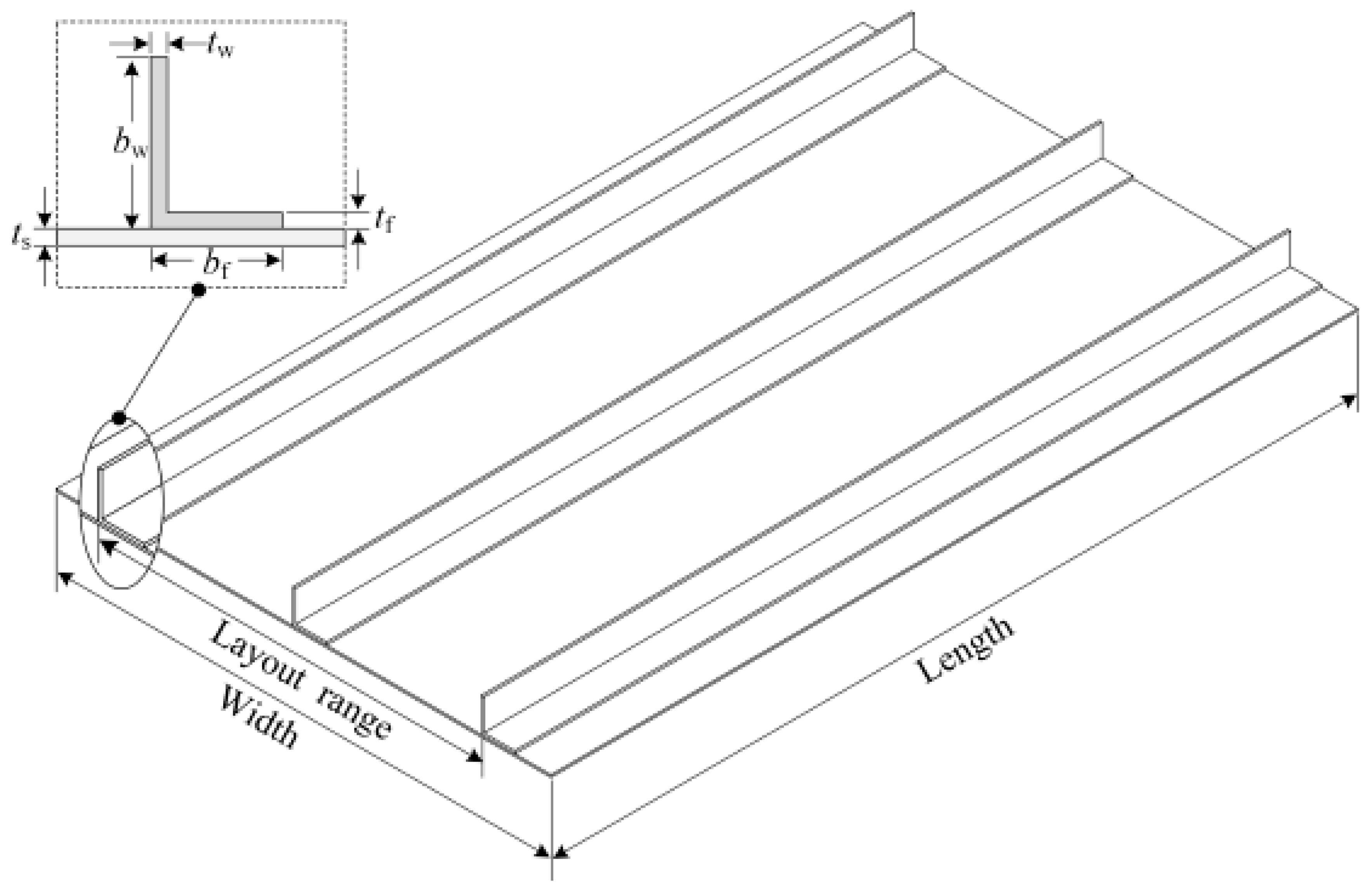
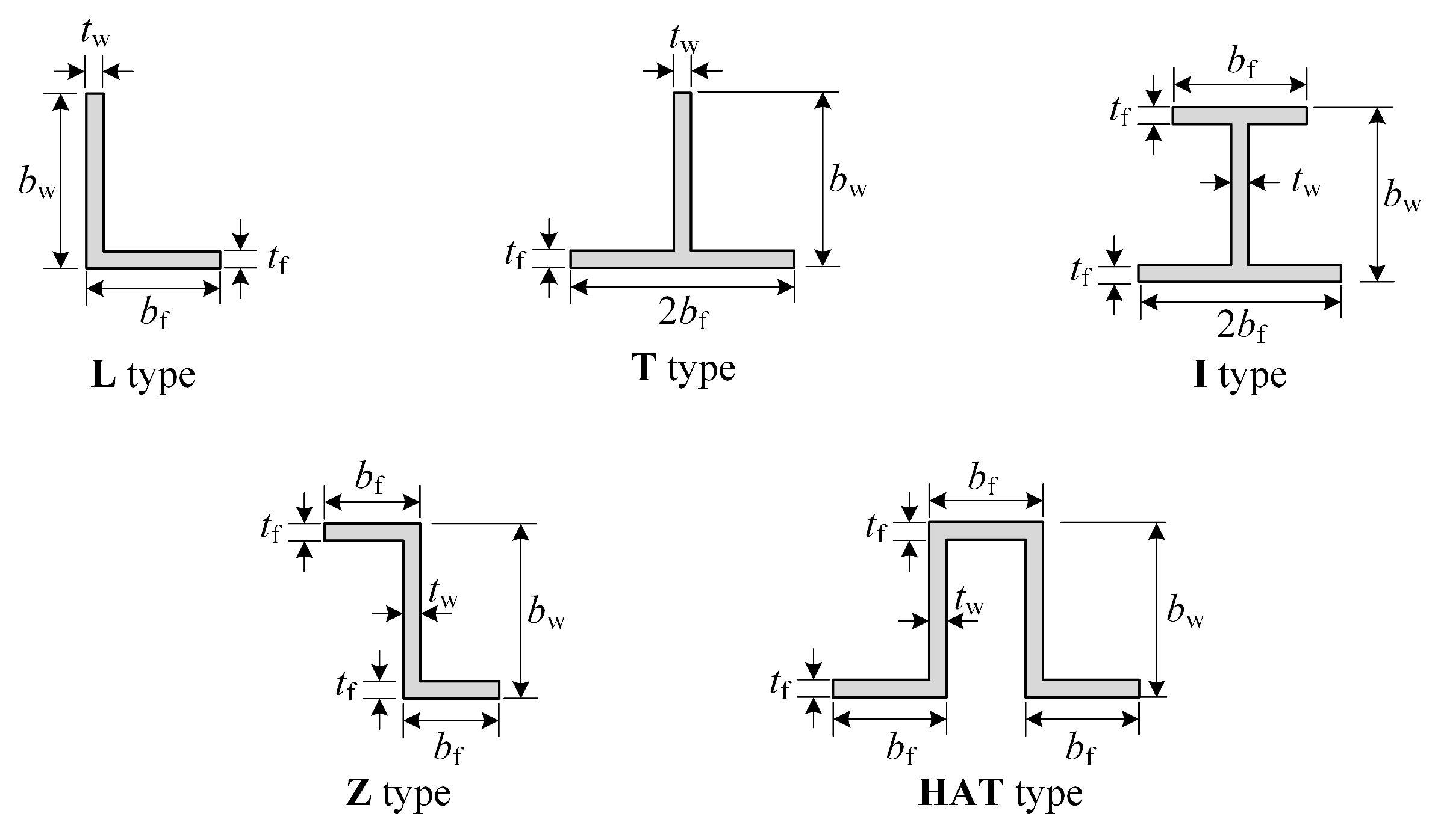
For the layout optimization problem of the stiffened plate, the length and width of the plate are given, and the optimization design variables include layout and size variables. The basic initial structure of the optimization problem presented in this paper is shown in Figure 1. The layout variables contain the position and section type of the stiffeners, as shown in Figure 2. Furthermore, the size variables include section size and skin thickness.

In general, the distribution of stiffeners is uniform, so that the number of stiffeners N is chosen as the position variable of stiffeners in the current work, at which point, the distribution spacing of stiffeners can be determined within the given layout range (shown in Figure 1), thus, both layout variables of the optimization problem are discrete and take values in discrete sets, while the size variables are all continuous, taking values in real numbers in the side constraints. Detailed information about the design variables is given in

Table 1. Description of design variables.

Classification	Symbol	Attribute	Description
Layout	N	Discrete	Stiffeners number
	T	Discrete	Stiffeners type
Size	$b_{\mathrm{w}}$	Continuous	Web width
	$b_{\mathrm{f}}$	Continuous	Flange width
	$t_{\mathrm{w}}$	Continuous	Web thickness
	$t_{\mathrm{f}}$	Continuous	Flange thickness
	$t_{\mathrm{s}}$	Continuous	Skin thickness

.

Therefore, the variables for layout optimization of metal stiffened plates can be stated as

$$\begin{array}{cc}\hfill \mathrm{find}& \mathbf{X}={\left[N,T,b_{\mathrm{w}},b_{\mathrm{f}},t_{\mathrm{w}},t_{\mathrm{f}},t_{\mathrm{s}}\right]}^{\mathrm{T}}\hfill \\ \hfill \mathrm{where}& N,T\in {\mathbb{N}}_{+}\hfill \\ \hfill & b_{\mathrm{w}},b_{\mathrm{f}},t_{\mathrm{w}},t_{\mathrm{f}},t_{\mathrm{s}}\in {\mathbb{R}}_{+}\hfill \end{array}$$

(1)

where, ${\mathbb{N}}_{+}$ and ${\mathbb{R}}_{+}$ denote the sets of positive integers and positive real numbers, respectively. Other notations can be found in Table 1.

2.2. Mathematical Model of Optimization Problem

In the present work, the static–dynamic coupled layout optimization problem of stiffened plates is divided into two disciplines, i.e., statics and dynamics. In the statics discipline, the objective function is to minimize the mass of the structure, and the constraints include static strength and stability. In the dynamics discipline, the objective function is to minimize the root mean square (RMS) of the maximum dynamic stress response of the structure, and the constraints include the structural frequency forbidden zone, the dynamic displacement response, and the structural mass. By transforming the disciplinary objectives into a single objective function with linear weighting, the mathematical model of the entire optimization problem can be stated as

$$\begin{array}{cc}\mathrm{find}\hfill & \mathbf{X}={\left[N,T,b_{\mathrm{w}},b_{\mathrm{f}},t_{\mathrm{w}},t_{\mathrm{f}},t_{\mathrm{s}}\right]}^{\mathrm{T}}\hfill \\ \min \hfill & W\left(\mathbf{X}\right)={\omega }^{\mathrm{T}}·\mathbf{F}\left(\mathbf{X}\right)\hfill \\ \mathrm{s}.\mathrm{t}.\hfill & g_{\sigma }\left(\mathbf{X}\right)=\sigma -\langle \sigma \rangle \le 0\hfill \\ \hfill & g_{\lambda }\left(\mathbf{X}\right)=\langle \lambda \rangle -\lambda \le 0\hfill \\ \hfill & g_{\widehat{d}}\left(\mathbf{X}\right)=\widehat{d}-\langle \widehat{d}\rangle \le 0\hfill \\ \hfill & g_m\left(\mathbf{X}\right)=m-\langle m\rangle \le 0\hfill \\ \hfill & f\notin \left[f^{\mathrm{L}},f^{\mathrm{U}}\right]\hfill \\ \hfill & \mathbf{X}\in \left[{\mathbf{X}}^{\mathrm{L}},{\mathbf{X}}^{\mathrm{U}}\right]\hfill \end{array}$$

(2)

where, $W\left(\mathbf{X}\right)$ is the weighted objective function, $\omega ={[{\omega }_{\mathrm{stat}},{\omega }_{\mathrm{dyna}}]}^{\mathrm{T}}$, in which ${\omega }_{\mathrm{stat}}$ and ${\omega }_{\mathrm{dyna}}$ are the weight coefficients of the statics and dynamics optimization objective functions, respectively, and the discipline objective $\mathbf{F}\left(\mathbf{X}\right)={[m,\widehat{\sigma }]}^{\mathrm{T}}$ contains the structural mass m and the RMS of the maximum dynamic stress response of the structure $\widehat{\sigma }$. The design variable $\mathbf{X}$ was discussed in the previous section, and the detailed description can be found in Table 1. $\sigma$ is the maximum static stress, $\lambda$ is the buckling factor, $\widehat{d}$ is the RMS of the maximum relative dynamic displacement response, f is the natural frequency, and the parameters wrapped by the symbol $\langle •\rangle$ indicate the limit values of the corresponding responses. Furthermore, ${\mathbf{X}}^{\mathrm{L}}$ and ${\mathbf{X}}^{\mathrm{U}}$ are the upper and lower bounds of $\mathbf{X}$, respectively, and $f^{\mathrm{L}}$ and $f^{\mathrm{U}}$ are the upper and lower bounds of the natural frequency forbidden zone of the structure, respectively.

3. Sub-Region Collaborative Optimization Method

3.1. Dynamic Driving Function

In the CO method, the system-level optimization is to obtain the global optimal solution under the interdisciplinary consistency constraint. To eliminate the influence of the order of magnitude and dimension, the relative change in the current disciplinary objective value to the initial value is taken as the overall objective, and to avoid no solution or convergency difficulties in system-level optimization, a relaxation factor is used for the consistency constraint, so that the system-level optimization model is defined as

$$\begin{array}{ccc}\hfill & \hfill \mathrm{find}& {\mathbf{Z}}^{\left(k\right)}={\left[N,T,b_{\mathrm{w}},b_{\mathrm{f}},t_{\mathrm{w}},t_{\mathrm{f}},t_{\mathrm{s}}\right]}^{\mathrm{T}}\hfill \\ \hfill & \hfill \min & W\left({\mathbf{Z}}^{\left(k\right)}\right)={\omega }_{\mathrm{stat}}\left|\frac{m^{\left(k\right)}}{m^{\left(0\right)}}\right|+{\omega }_{\mathrm{dyna}}\left|\frac{{\widehat{\sigma }}^{\left(k\right)}}{{\widehat{\sigma }}^{\left(0\right)}}\right|\hfill \\ \hfill & \hfill \mathrm{s}.\mathrm{t}. & J_i\left({\mathbf{Z}}^{\left(k\right)}\right)={∥{\mathbf{Z}}^{\left(k\right)}-{\mathbf{X}}_i^{\left(k\right)*}∥}_2\le {\epsilon }_i\hfill \end{array}$$

(3)

where $i=1,2$ represent the statics and dynamics disciplines (subsystems), respectively. $m^{\left(k\right)}$ and ${\widehat{\sigma }}^{\left(k\right)}$ are the disciplinary objective values for the kth system-level optimization of statics and dynamics, respectively, $m^{\left(0\right)}$ and ${\widehat{\sigma }}^{\left(0\right)}$ are reasonable initial values of disciplinary objectives, $J_i$ is the interdisciplinary consistency constraint, expressed in the Euclidean norm, $\epsilon$ is the consistency constraint relaxation factor, ${\mathbf{X}}_i^{\left(k\right)*}$ is the optimal value of the design variable at the subsystem level, and ${\mathbf{Z}}^{\left(k\right)}$ is the system-level design variable.

According to the basic idea of the CO method, the statics/dynamics subsystem-level optimization model should be formulated as

$$\begin{array}{ccc}\hfill & \hfill \mathrm{find}& {\mathbf{X}}_i^{\left(k\right)}={\left[N,T,b_{\mathrm{w}},b_{\mathrm{f}},t_{\mathrm{w}},t_{\mathrm{f}},t_{\mathrm{s}}\right]}^{\mathrm{T}}\hfill \\ \hfill & \hfill \min & J_i\left({\mathbf{X}}_i^{\left(k\right)}\right)={∥{\mathbf{X}}_i^{\left(k\right)}-{\mathbf{Z}}^{\left(k\right)*}∥}_2\hfill \\ \hfill & \hfill \mathrm{s}.\mathrm{t}. & {\mathbf{g}}_i\left({\mathbf{X}}_i^{\left(k\right)}\right)\le 0\hfill \\ \hfill & & {\mathbf{X}}_i^{\left(k\right)}\in \left[{\mathbf{X}}^{\mathrm{L}},{\mathbf{X}}^{\mathrm{U}}\right]\hfill \end{array}$$

(4)

where the inequality constraint ${\mathbf{g}}_i$ represents the local constraint in the statics/dynamics subsystem, ${\mathbf{X}}_i^{\left(k\right)}$ is the subsystem-level design variable, and ${\mathbf{Z}}^{\left(k\right)*}$ represents the optimal value of the design variable at the system level.

However, the standard CO method often finds a feasible solution instead of an optimal solution. The reason for this is not only the failure of the KKT stationary condition due to the consistency constraint mentioned by Alexandrov [22], but also the reason for the dominance of the consistency constraint in the game process of “consistency” and “feasibility”, which makes the system-level optimization exceptionally hard to converge and has very poor robustness, especially when the optimization process enters the feasible region.

To address the difficulty of the iteration of the CO method in the feasible region, the following dynamic driving function (DDF) is added to the objective function (interdisciplinary consistency information $J_i$) of the subsystem

$$F_{\mathrm{d}}=\kappa ·\left|\frac{F_i^k}{F_i^0}\right|$$

(5)

where

$$\kappa =\left\{\begin{array}{ccc}\hfill a+\frac{c}{k^b}\hfill & \hfill & \mathrm{In}\mathrm{the}\mathrm{feasible}\mathrm{region}\hfill \\ 0\hfill & \hfill & \mathrm{Out}\mathrm{of}\mathrm{the}\mathrm{feasible}\mathrm{region}\hfill \end{array}\right.$$

where k is the number of system-level iterations, $F_i$ is the statics/dynamics disciplinary objectives, i.e., m and $\widehat{\sigma }$. $\kappa$ is the driving factor, and a, b, and c are constant coefficients. Within the feasible region, $\kappa$ is a strictly monotone decreasing function with a as the limit, b used to control the decay rate, and c used to control the initial value.

The significance of adding the dynamic driving function is to prevent the optimization process of the subsystem entering the feasible region from stagnation. The significance of decay is to prevent “feasibility” from dominating in the later stage of optimization, which may lead to system-level coordination difficulties. The specific performance of the dynamic driving function is discussed in Section 4.

Therefore, by adding the dynamic driving function Equation (5) into Equation (4), the optimization model of the statics subsystem becomes

$$\begin{array}{ccc}\hfill & \hfill \mathrm{find}& {\mathbf{X}}_1^{\left(k\right)}\hfill \\ \hfill & \hfill \min & {\Phi }_1({\mathbf{X}}_1^{\left(k\right)},m^{\left(k\right)})=J_1\left({\mathbf{X}}_1^{\left(k\right)}\right)+F_{\mathrm{d}}\left(m^{\left(k\right)}\right)\hfill \\ \hfill & \hfill & ={∥{\mathbf{X}}_1^{\left(k\right)}-{\mathbf{Z}}^{\left(k\right)*}∥}_2+{\kappa }_1·\left|\frac{m^{\left(k\right)}}{m^{\left(0\right)}}\right|\hfill \\ \hfill & \hfill \mathrm{s}.\mathrm{t}. & g_{\sigma }\left({\mathbf{X}}_1^{\left(k\right)}\right)\le 0\hfill \\ \hfill & \hfill & g_{\lambda }\left({\mathbf{X}}_1^{\left(k\right)}\right)\le 0\hfill \\ \hfill & \hfill & {\mathbf{X}}_1^{\left(k\right)}\in \left[{\mathbf{X}}^{\mathrm{L}},{\mathbf{X}}^{\mathrm{U}}\right]\hfill \end{array}$$

(6)

and the optimization model of the dynamics subsystem becomes

$$\begin{array}{ccc}\hfill & \hfill \mathrm{find}& {\mathbf{X}}_2^{\left(k\right)}\hfill \\ \hfill & \hfill \min & {\Phi }_2({\mathbf{X}}_2^{\left(k\right)},{\widehat{\sigma }}^{\left(k\right)})=J_2\left({\mathbf{X}}_2^{\left(k\right)}\right)+F_{\mathrm{d}}\left({\widehat{\sigma }}^{\left(k\right)}\right)\hfill \\ \hfill & \hfill & ={∥{\mathbf{X}}_2^{\left(k\right)}-{\mathbf{Z}}^{\left(k\right)*}∥}_2+{\kappa }_2·\left|\frac{{\widehat{\sigma }}^{\left(k\right)}}{{\widehat{\sigma }}^{\left(0\right)}}\right|\hfill \\ \hfill & \hfill \mathrm{s}.\mathrm{t}. & g_{\widehat{d}}\left({\mathbf{X}}_2^{\left(k\right)}\right)\le 0\hfill \\ \hfill & \hfill & g_m\left({\mathbf{X}}_2^{\left(k\right)}\right)\le 0\hfill \\ \hfill & \hfill & {\mathbf{X}}_2^{\left(k\right)}\in \left[{\mathbf{X}}^{\mathrm{L}},{\mathbf{X}}^{\mathrm{U}}\right]\hfill \end{array}$$

(7)

3.2. Sub-Region Decomposition

The design variables for both statics and dynamics disciplines are shared variables, and this implies that the difficulty of the optimization problem is reduced, but the dimensionality is increased exponentially through disciplinary decomposition. It is also worth noting that within the statics and dynamics subsystems, the design variables can be strictly separated according to the optimization region.

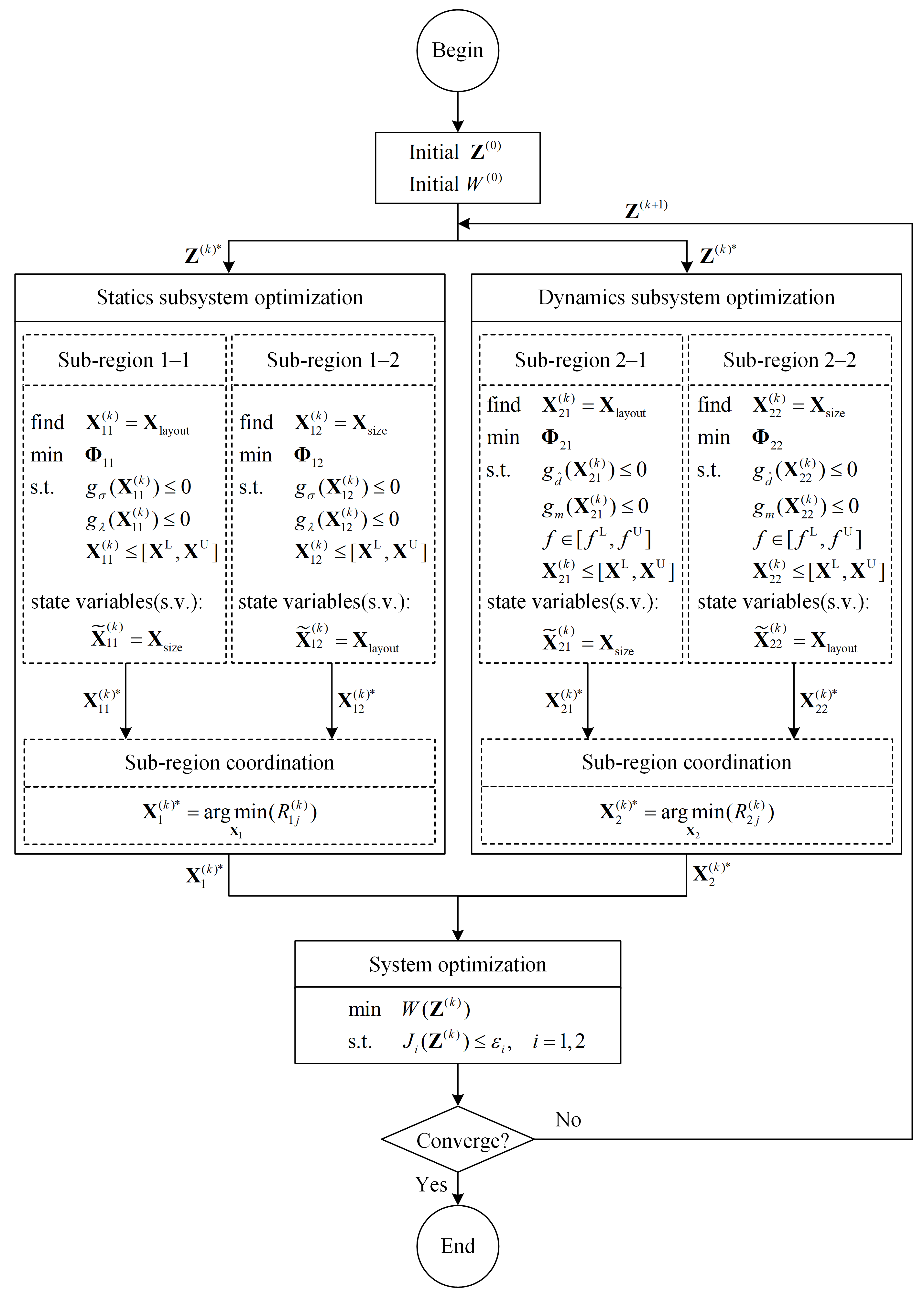
Theoretically, the MDO method prefers a methodology where the type of decomposition is not limited to disciplines, but can also be based on structures or task processes [23]. Using the characteristics of layout optimization, the structure can be further decomposed into sub-regions embedded in the subsystem according to the structure optimization region, and each sub-region can be optimized in parallel, and different optimization algorithms can be selected. Such is the concept underlying the sub-region collaborative optimization (CSRC) method proposed in this paper, and its optimization strategy is shown in Figure 3 (in the subsequent content, the subscript i represents the corresponding subsystem, and j represents the corresponding sub-region). Therefore, strictly speaking, the present method is still a two-level optimization method.

In Figure 3, the state variable ${\tilde{\mathbf{X}}}_{ij}^{\left(k\right)}$ represents the quantity that remains constant during the optimization process of this sub-region. The optimization objective function for each sub-region is the interdisciplinary consistency information containing the driving function

$$\begin{array}{lll}{\Phi }_{ij}({\mathbf{X}}_{ij}^{\left(k\right)},F_i^{\left(k\right)})& =& {\eta }_j·J_{ij}\left({\mathbf{X}}_{ij}^{\left(k\right)}\right)+F_{\mathrm{d}}\left(F_i^{\left(k\right)}\right)\\ & =& {\eta }_j·{∥{\mathbf{X}}_{ij}^{\left(k\right)}-{\mathbf{Z}}^{\left(k\right)*}∥}_2+\\ & & {\kappa }_i·\left|\frac{F_i^{\left(k\right)}}{F_i^{\left(0\right)}}\right|\end{array}$$

(8)

where ${\eta }_j$ is the correction factors of the discrete variable, taking ${\eta }_1=0.1$ and ${\eta }_2=1$ in this paper, and it is used to correct for the influence of discrete variables in the layout sub-region on interdisciplinary consistency information.

Similarly, the discrete variable correction factor needs to be added to the consistency constraints of the system-level optimization model, so that Equation (3) becomes

$$J_i\left({\mathbf{Z}}^{\left(k\right)}\right)=\sum _{j=1}^2{\eta }_j·{∥{\mathbf{Z}}^{\left(k\right)}-{\mathbf{X}}_{ij}^{\left(k\right)*}∥}_2\le {\epsilon }_i$$

(9)

where the correction factor is consistent with Equation (8).

3.3. Sub-Region Coordination

The sub-region coordination function $R_{ij}^{\left(k\right)}$ in Figure 3 is presented as

$$R_{ij}^{\left(k\right)}=F_i\left(\mathbf{X}\right)+\Theta ·\sum \left[max\left(\phi \left(\mathbf{X}\right)-\zeta ,0\right)\right]$$

(10)

where

$$\begin{array}{cc}\hfill & \phi \left(\mathbf{X}\right)=\frac{g\left(\mathbf{X}\right)}{\langle g\rangle }\hfill \\ \hfill & \mathbf{X}\in \left\{{\mathbf{X}}_{ij}^{\left(k\right)*},{\mathbf{X}}_{i,\mathrm{sov}}^{\left(k\right)}\right\}\hfill \end{array}$$

(11)

In Equation (10), $F_i$ is the optimization objective of the ith subsystem, i.e., m and $\widehat{\sigma }$, $\Theta$ is a sufficiently large penalty coefficient, $\phi$ is the regularized constraint violation, and $\zeta$ is the constraint tolerance, taken as $\zeta =0.005$. In Equation (11), g is the constraint value, and $\langle g\rangle$ is the constrain allowable value, as shown in Equation (2).

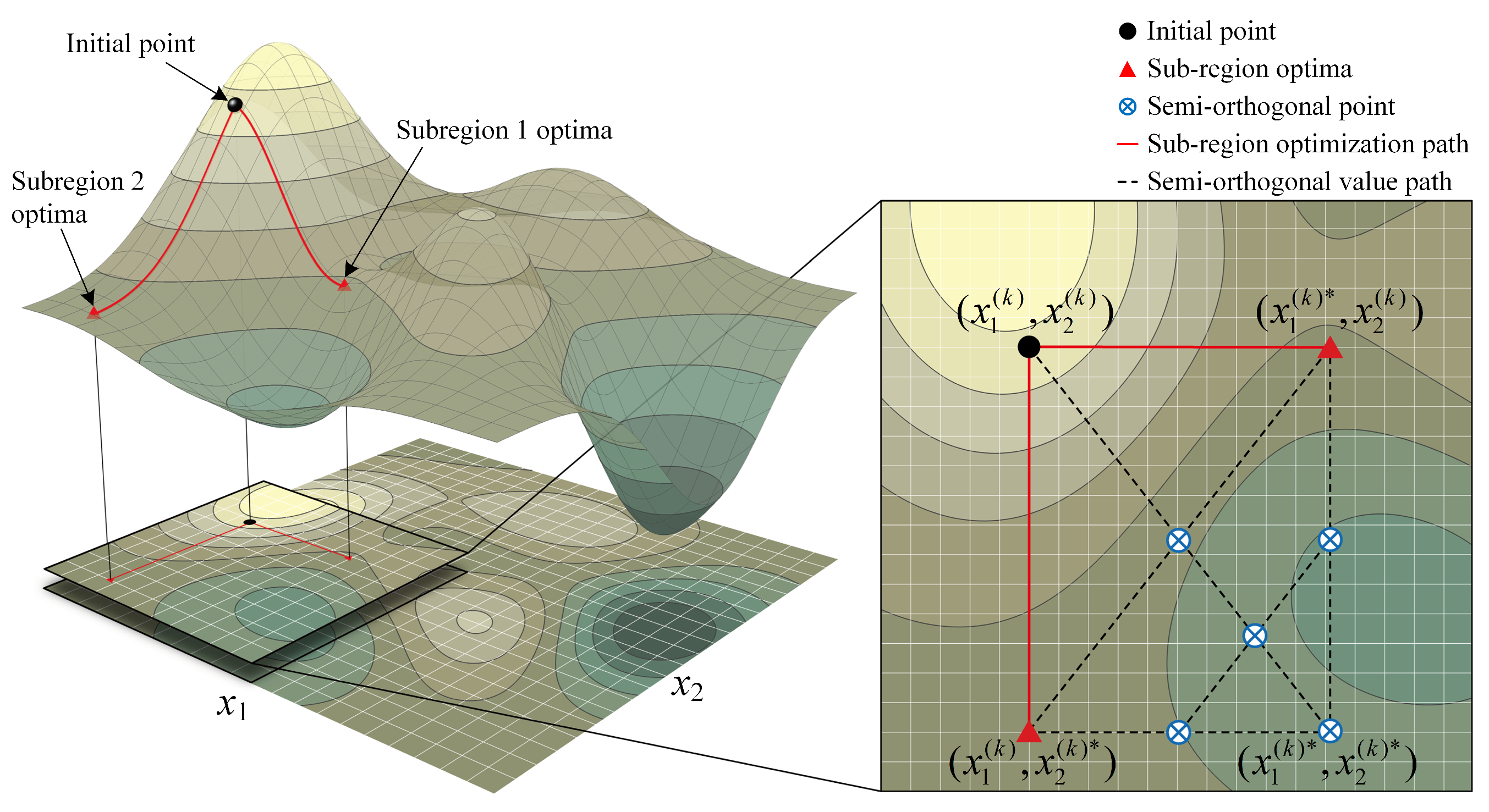
${\mathbf{X}}_{i,\mathrm{sov}}^{\left(k\right)}$ is the semi-orthogonal value (SOV) vector based on the initial and optimal values of the sub-region. Take the two-factor case as an example to introduce the SOV vector, as shown in Figure 4. The SOV is the point represented by the symbol ⊗ in Figure 4, and the SOV points without coordinates are the midpoints of the other two points, which are easy to understand and will not be repeated here, and the so-called “semi-orthogonal” is just like its literal meaning. The variable values of the five SOV points are taken into Equation (10), and the results are then compared with the results of Equation (10) for the optimal point of the sub-regions. The design variables that minimize $R_{ij}^{\left(k\right)}$ are transferred to the system level. In particular, when the layout variable has a special case, that is, when the mid-value is a non-integer, rounding is performed, and the duplicate value is deleted. From the above, it is clear that the sub-region coordination in the two-factor case requires, at most, five discipline analyses to obtain a coordinated solution.

In fact, sub-region coordination is not intended to find the optimal solution in a single coordination, but only to accelerate the optimization process by performing a semi-orthogonal design of experiment (DOE) on a region composed of the design variables before and after the sub-region optimization. Compared with the coordination by comparing only the optimal solutions of two sub-regions, the optimization process with sub-region coordination converges more rapidly.

3.4. Adaptive Surrogate Model Based on Benchmark Sub-Region

The surrogate model is one of the key techniques for MDO, which is a comprehensive modeling technique including the design of experiment (DOE) and approximation method. The approximate methods mainly include the polynomial response surface model (RSM), Kriging model, radial basis function neural network (RBF) model, etc. In terms of computational effort, the Kriging model is the largest, followed by the RBF model, and the RSM is the smallest. However, for the dynamic response, the prediction accuracy of RSM is extremely low. Therefore, based on the tradeoff between accuracy and computational effort, the quadratic RSM approximation is chosen for the statics subsystem and the RBF approximation for the dynamics subsystem in the current work. However, the approximation accuracy for the whole subsystem is undesirable because changes in discrete variables can lead to abrupt changes in structural properties and responses. Therefore, an adaptive surrogate model (ASM) based on the special form of sub-region decomposition is proposed in this paper.

The ASM is to divide the DOE points of the whole subsystem and construct several small surrogate models according to a certain sub-region, which is called the benchmark region here. The sub-region can autonomously select the surrogate model to be called for this optimization by the parameters transmitted from the system level, which is one of the reasons for the so-called “adaptive”. These adaptive sub-region surrogate models (ASSM) are characterized by fewer design variables, higher prediction accuracy, and fewer DOE points. The layout sub-region, due to its discrete nature, is chosen as the benchmark region for distinguishing the ASM in the present work.

Benefiting from the SOV of sub-region coordination, i.e., each sub-region coordination is equivalent to a semi-orthogonal DOE, so that the results of SOV disciplinary analysis can be stored in the ASM database for updating, which is the second reason for the “adaptive”. The framework and interaction logic of ASM is shown in Figure 5, where SO stands for system-level optimization, SRO represents sub-region optimization, and ASSM represents adaptive sub-region surrogate model.

The steps for constructing the ASM are as follows:

Step 1. 

Constructing the initial database according to the experimental design method (optimal Latin hypercube design in current work).

Step 2. 

Partitioning the original database into several smaller databases by dividing the DOE points according to discrete variables.

Step 3. 

Initializing the ASSMs by DOE points in the database, which constitutes the initial ASM.

Step 4. 

Storing the SOV data in the database after each round of sub-region coordination.

Step 5. 

Updating the ASM before the next round of system optimization and sub-region optimization.

From the above steps, it can be understood that after the initial ASM is built, each round of optimization only involves disciplinary analysis for the SOV points in Section 3.3 to update the ASM, and the rest of the optimization process is solved by invoking the surrogate model.

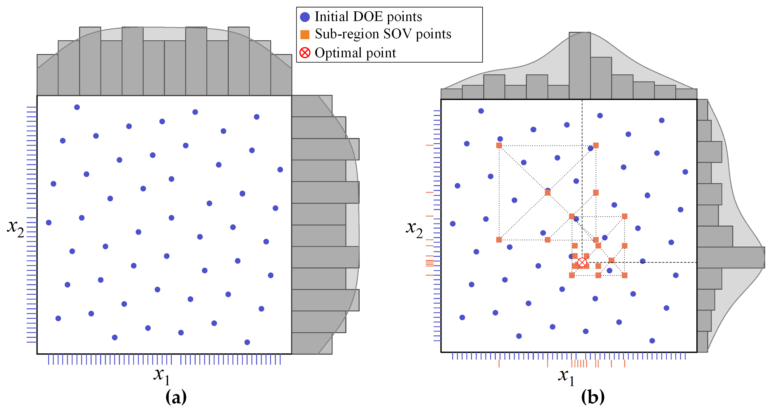
The data point distribution of the two-factor ASM is given in Figure 6. Obviously, the disciplinary analysis results of sub-region coordination are reused to update the ASM, and since each sub-region coordination is taken semi-orthogonally, it is equivalent to performing an adaptive DOE for each coordination, and the closer to the optimal point, the higher the accuracy of the ASM.

4. Illustrative Example of Dynamic Driving Function

A numerical example [24], commonly used in MDO, is used to illustrate the superiority of the dynamic driving function in Section 3.1.

$$\begin{array}{ccc}\hfill & \min \hfill & f\left(\mathbf{x}\right)=x_1^2+x_2^2\hfill \\ \hfill & \mathrm{s}.\mathrm{t}.\hfill & g_1\left(\mathbf{x}\right)=x_1+\beta x_2-4\le 0\hfill \\ \hfill & & g_2\left(\mathbf{x}\right)=2-\beta x_1-x_2\le 0\hfill \end{array}$$

(12)

where $\beta =0.1$, and the theoretical optimal solution is $\mathbf{x}=(0.198,1.980)$ and $f\left(\mathbf{x}\right)=3.9596$.

The system and subsystem levels, after decomposition according to the relaxation CO method, are as follows:

(a)

System level

$$\begin{array}{ccc}\hfill & \min \hfill & f\left(\mathbf{z}\right)=z_1^2+z_2^2\hfill \\ \hfill & \mathrm{s}.\mathrm{t}. \hfill & J_1^{*}\left(\mathbf{z}\right)={(z_1-x_{11}^{*})}^2+{(z_2-x_{12}^{*})}^2\le \epsilon \hfill \\ \hfill & & J_2^{*}\left(\mathbf{z}\right)={(z_1-x_{21}^{*})}^2+{(z_2-x_{22}^{*})}^2\le \epsilon \hfill \end{array}$$

(13)

(b)

Subsystem 1

$$\begin{array}{ccc}\hfill & \min \hfill & J_1\left({\mathbf{x}}_1\right)={(x_{11}-z_1^{*})}^2+{(x_{12}-z_2^{*})}^2\hfill \\ \hfill & \mathrm{s}.\mathrm{t}. \hfill & g_1\left({\mathbf{x}}_1\right)=x_{11}+0.1x_{12}-4\le 0\hfill \end{array}$$

(14)

(c)

Subsystem 2

$$\begin{array}{ccc}\hfill & \min \hfill & J_2\left({\mathbf{x}}_2\right)={(x_{21}-z_1^{*})}^2+{(x_{22}-z_2^{*})}^2\hfill \\ \hfill & \mathrm{s}.\mathrm{t}. \hfill & g_2\left({\mathbf{x}}_2\right)=-0.1x_{21}-x_{22}+2\le 0\hfill \end{array}$$

(15)

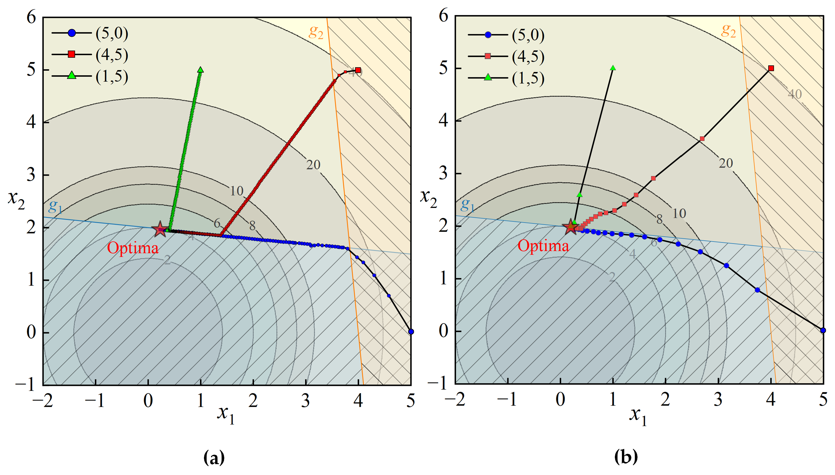
Three initial points are selected, where point $(5,0)$ is in fully infeasible regions, point $(4,5)$ is in the partially infeasible region, and point $(1,5)$ is in the fully feasible region. The relaxation CO method and the CO method with dynamic driving function are used to optimize the problem, and the iteration path is shown in Figure 7, where the constant coefficients $a=0$, $b=2$, and $c=1$ in the DDF Equation (5) and the relaxation factor $\epsilon =0.001$ in Equation (13) are taken in this example. The comparison of optimization results is shown in

Table 2. Comparison of optimization results at different initial points.

Method	Initial Points	Optimum	Objective	Iterations
Relaxation CO	$(5,0)$	$(0.2287,1.9520)$	3.8627 *	77
	$(4,5)$	$(0.3600,1.9333)$	3.8674 *	240
	$(1,5)$	$(0.3613,1.9332)$	3.8678 *	112
Relaxation CO with DDF	$(5,0)$	$(0.1981,1.9821)$	3.9676	19
	$(4,5)$	$(0.1976,1.9524)$	3.8509 *	25
	$(1,5)$	$(0.1987,1.9853)$	3.9811	10

* Constraints are not fully satisfied due to relaxation and constraint tolerance, so the objective value looks smaller.

. As can be seen, it is difficult for the CO method to converge to the optimal solution due to the small step size after entering the feasible region. On the contrary, the number of iterations is reduced significantly, and the robustness is improved remarkably by adding the DDF, as shown in Figure 7b and Table 2.

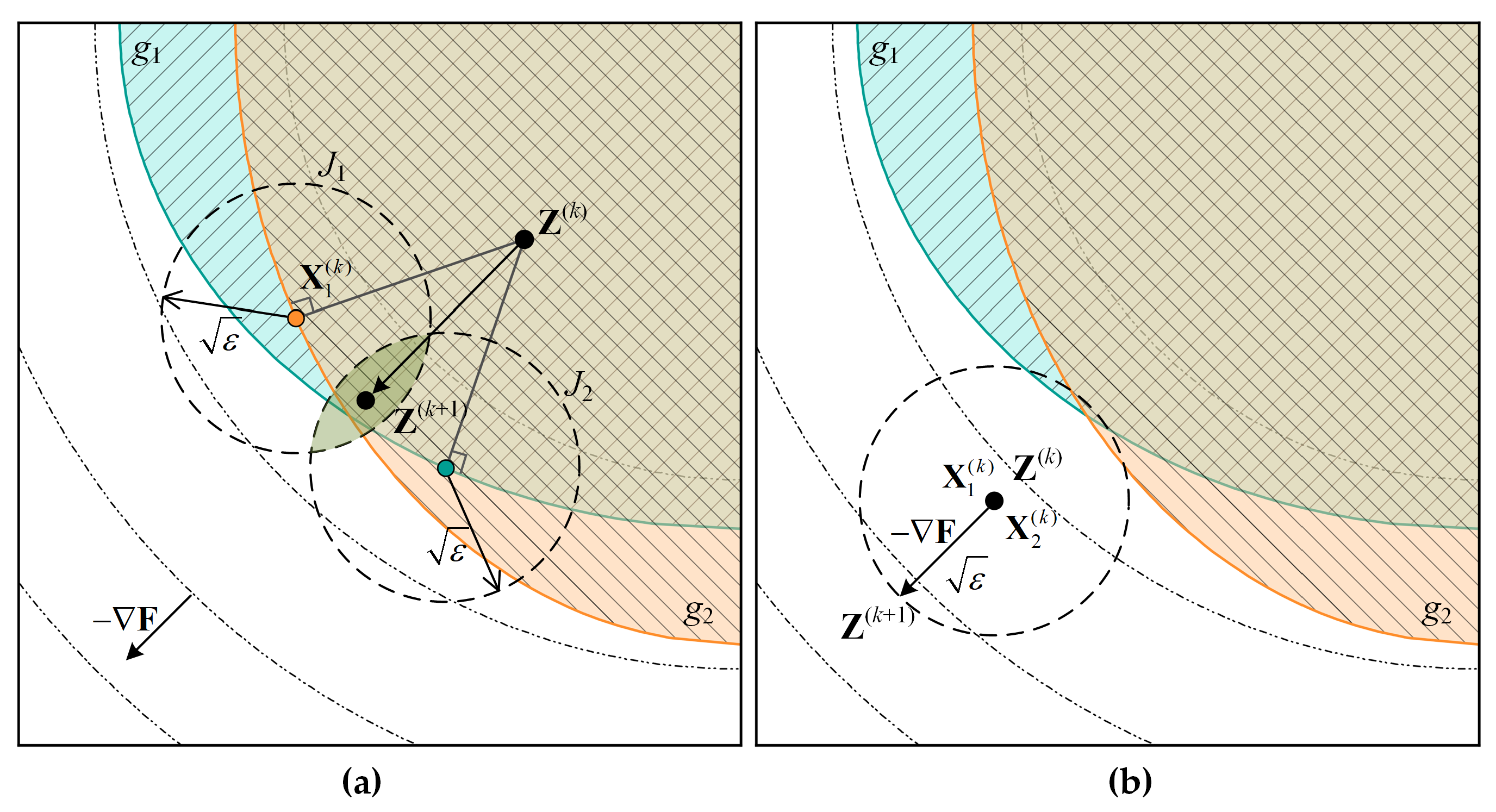
In order to explain this behavior more graphically, two subsystems are analyzed using the geometric method, giving a schematic representation of the optimization process of the CO method, as shown in Figure 8.

In Figure 8a, the kth iteration starting point ${\mathbf{Z}}^{\left(k\right)}$ at the system level is inside the fully infeasible region, at which time the optimal point of the subsystem is definitely the point with the shortest distance from ${\mathbf{Z}}^{\left(k\right)}$ on $g_1=0/g_2=0$. The consistency constraint is expressed as a circle with the square root of the relaxation factor $\sqrt{\epsilon }$ as the radius, and the area of the circle superposition is the search area for system-level optimization. As can be seen, the optimization efficiency of the CO method is considerable when the starting point of the iteration lies outside the feasible region.

In Figure 8b, the kth iteration starting point ${\mathbf{Z}}^{\left(k\right)}$ at the system level is within the feasible region, at which time the optimal step size of the iteration is equal to $\sqrt{\epsilon }$ (it should actually include the constraint tolerance of the optimizer, which is generally extremely small and is ignored here). The range of the circle representing the relaxation factor is deliberately enlarged for clarity, while in practice, the step size in the feasible region is tiny. In other words, in the feasible region, “consistency” is absolutely dominant, and subsystem optimization stagnates, leaving system optimization as the sole driver of the entire optimization problem.

This simple numerical test illustrates the superiority of the DDF, which not only greatly improves the optimization efficiency, but also the stability of the CO method.

5. Optimization of Metal Stiffened Plate

5.1. Problem Description

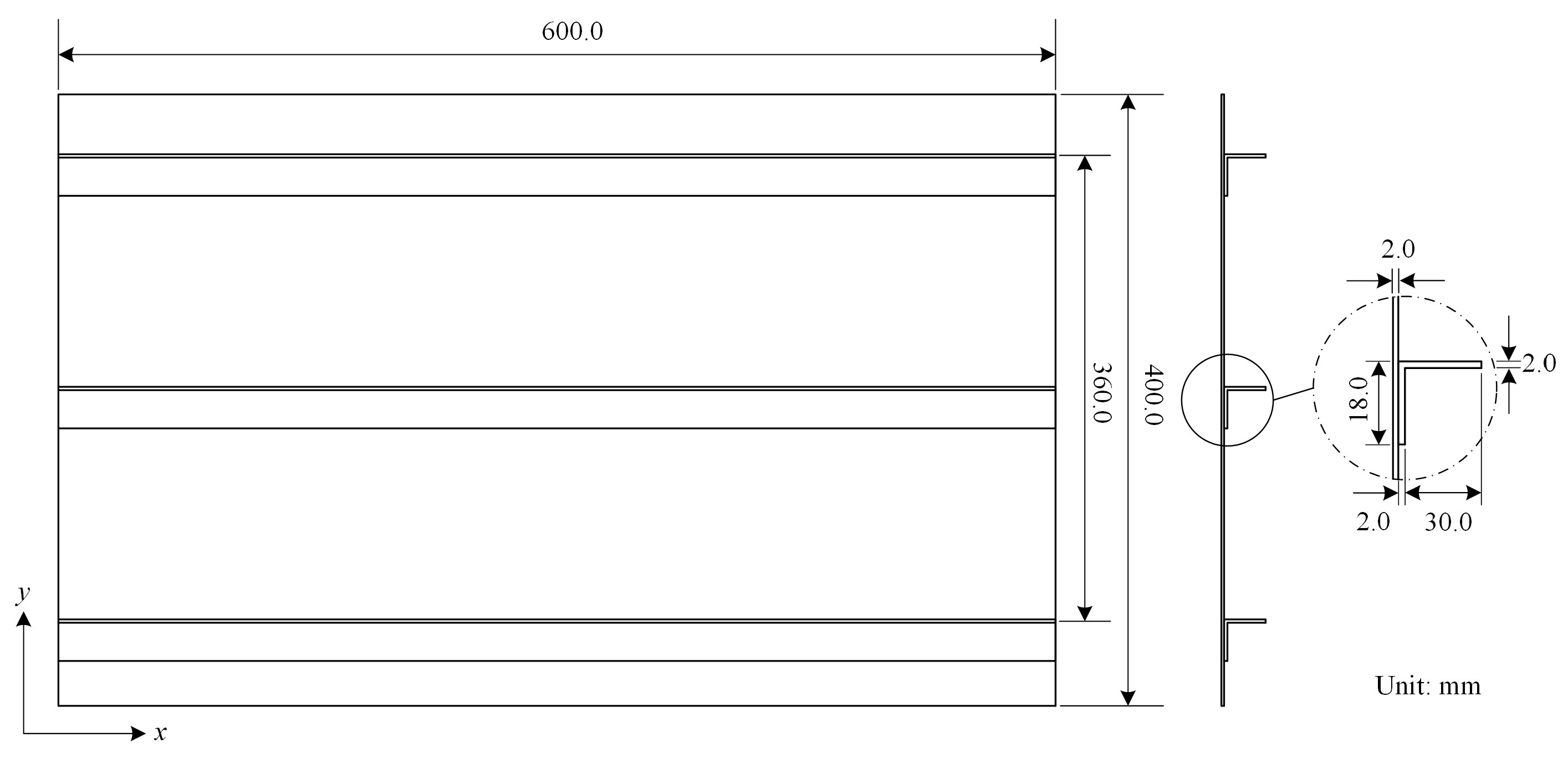
The stiffened plate structure studied by Murphy et al. [25] is taken as the prototype for the layout optimization subjected to static and dynamic loads. The plate is 600 mm long and 400 mm wide, and the layout range is 360 mm at the middle of the short side. The material used for the plate is 2024-T351 aluminum alloy with a modulus of elasticity of 71 GPa, Poisson’s ratio of 0.33, and density of 2700 kg/m${}^3$.Three initial sets of values were chosen as the starting point for optimization to verify the robustness of the method. In addition, a sequential optimization method described in the literature [26] was chosen to perform an additional optimization, using Case 1 as the starting point, which can be compared with the CSRC method to demonstrate the reduction in “wall-clock time” due to concurrent mechanisms. See

Table 3. Variables range and initial value.

Variables	Unit	Range	Initial Points			Sequential Method
			Case 1	Case 2	Case 3
N	-	{2,3,4,5,6}	3	5	6	3
T	-	{1,2,3,4,5}	1	3	5	1
$b_{\mathrm{w}}$	mm	[20.0, 30.0]	30.00	25.00	30.00	30.00
$b_{\mathrm{f}}$	mm	[6.0, 18.0]	18.00	12.00	18.00	18.00
$t_{\mathrm{w}}$	mm	[0.8, 2.0]	2.00	2.00	1.40	2.00
$t_{\mathrm{f}}$	mm	[0.8, 2.0]	2.00	2.00	1.40	2.00
$t_{\mathrm{s}}$	mm	[0.8, 2.0]	2.00	2.00	1.40	2.00

for detailed information on design variables. The stiffener section types (T) 1, 2, 3, 4, and 5 correspond to L, T, I, Z, and Hat type, respectively. The specific stiffener section types are shown in Figure 2, and the initial geometric model and dimensions of Case 1 are shown in Figure 9.

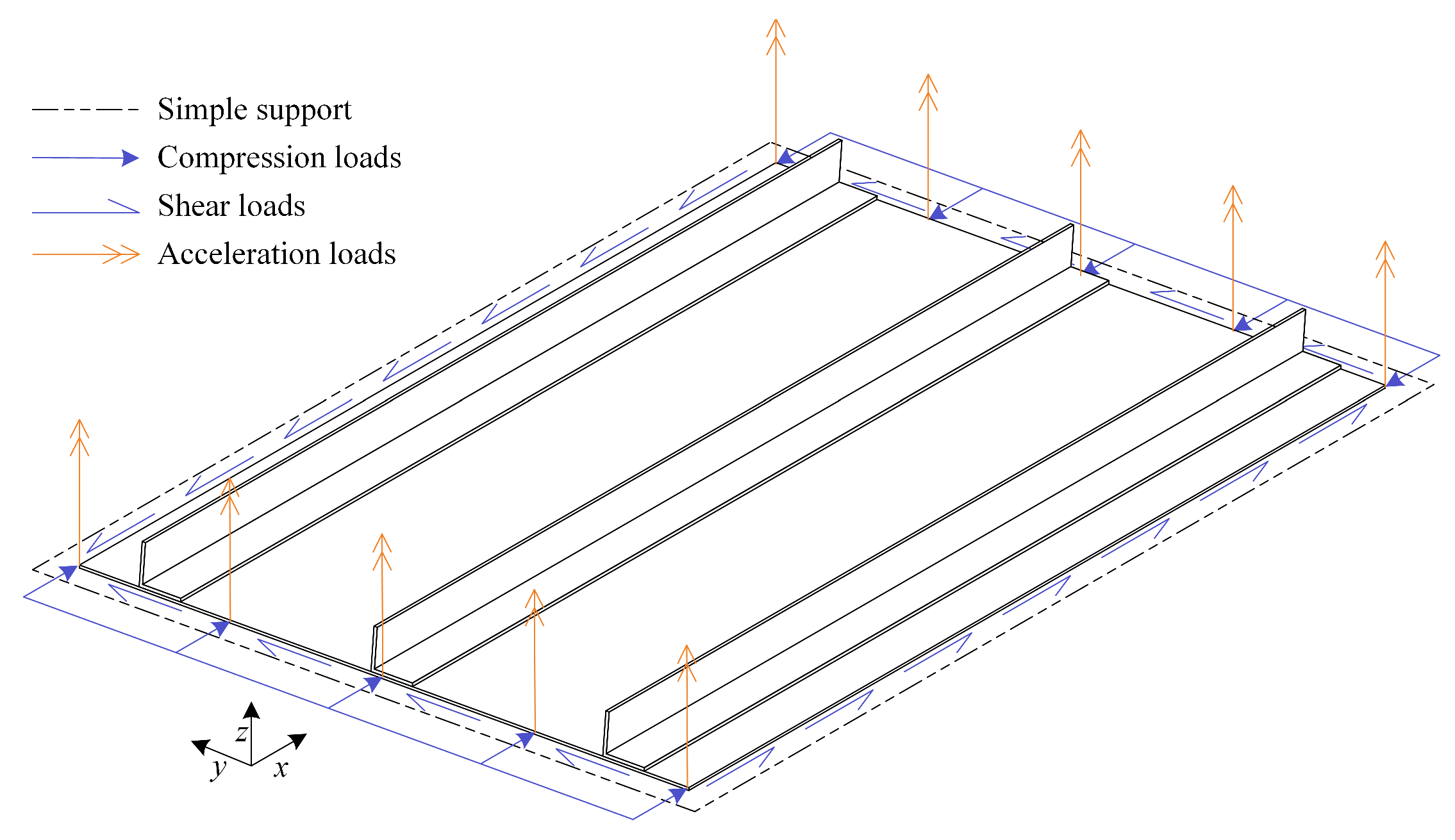
The stiffened plate is subject to static and dynamic load cases, respectively, and is simply supported on four sides, as shown in Figure 10.

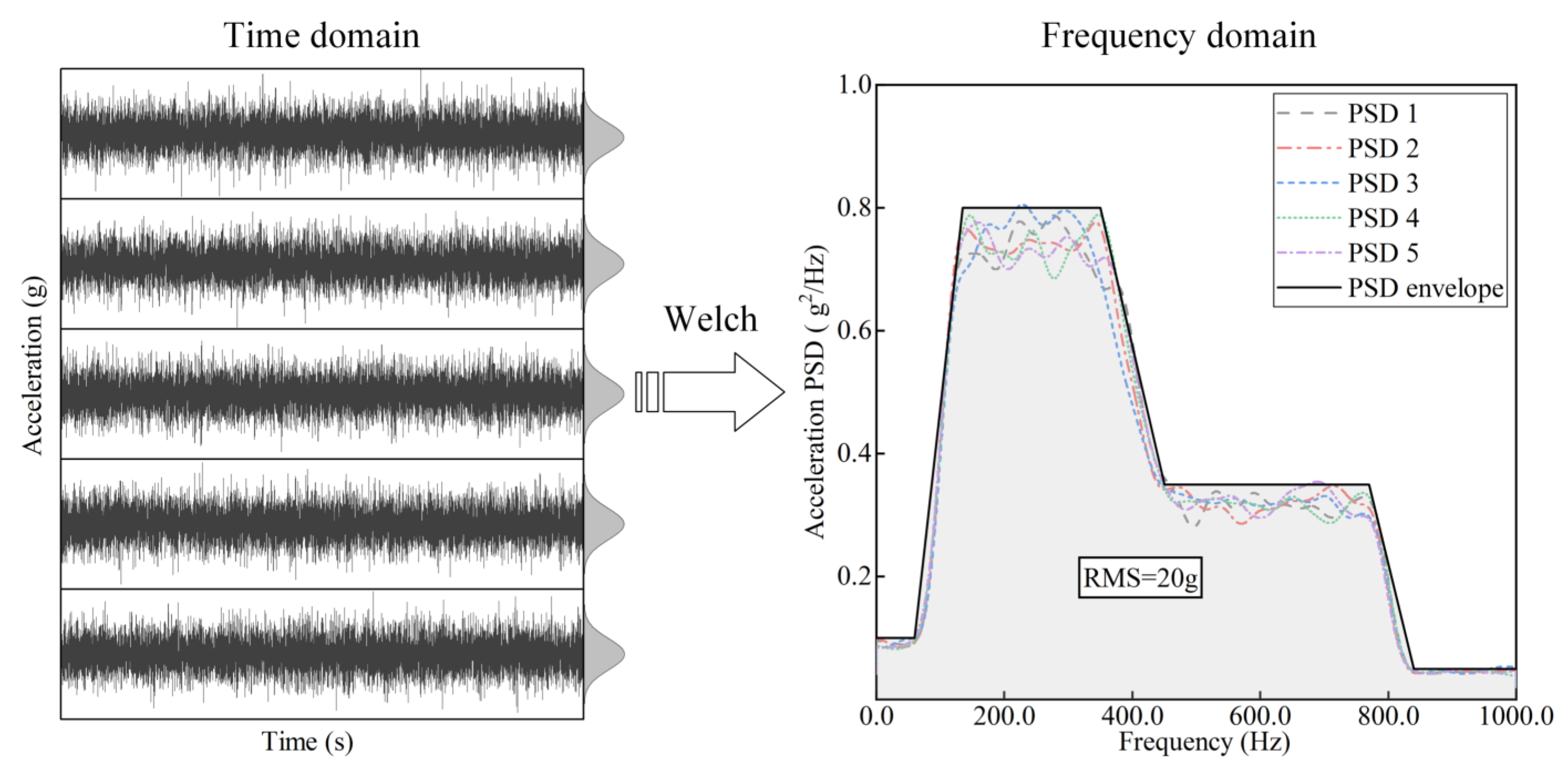
Under the static load case, the stiffened plate is subjected to a uniform compression-shear combined load, in which the axial compression load on the short sides is 30 kN, and the shear load on the four sides is 15 kN, while under the dynamic load case, the short side of the plate is subjected to random foundation acceleration excitation in the z-direction, with a cut-off frequency of [0.1, 1000] Hz and a modal damping of 0.03. The power spectral density (PSD) was estimated using the Welch method based on five sets of random acceleration time-domain load signals, and a standard PSD envelope curve with a root mean square (RMS) of 20 g was established, as shown in Figure 11.

In the statics optimization, the optimization objective is to minimize the structural mass m, the structural stability constraint is the buckling factor $\langle \lambda \rangle =1$, and the static strength constraint is $\langle \sigma \rangle =325\mathrm{MPa}$. In the dynamics optimization, the optimization objective is to minimize the RMS of the maximum dynamic stress response of the structure $\widehat{\sigma }$, the structural weight constraint $\langle m\rangle =2.0\mathrm{kg}$, the structural frequency forbidden zone $[f^{\mathrm{L}},f^{\mathrm{U}}]=[180,250]\mathrm{Hz}$, and the RMS of the maximum relative dynamic displacement response $\langle \widehat{d}\rangle =0.5\mathrm{mm}$.

5.2. Results and Discussion

Multi-island genetic algorithm (Multi-Island GA in Isight) is chosen for layout sub-region optimization, while sequential quadratic programming (NLPQLP in Isight) based on the adaptive surrogate model and mixed integer sequential quadratic programming (MISQP in Isight) are chosen for size sub-region optimization and system-level optimization, respectively. The call and automatic update of the adaptive surrogate model are implemented by Jython, which is a built-in programming language in Isight, and the disciplinary analysis is performed by calling MSC.Patran in the PCL, which is a built-in programming language in Patran. All same-level steps in the CSRC method can be executed concurrently in Isight, with high efficiency. The CPU of the computer used for optimization in this paper is a 32-core Intel(R) Xeon(R) Gold 6242R @3.10 GHz.

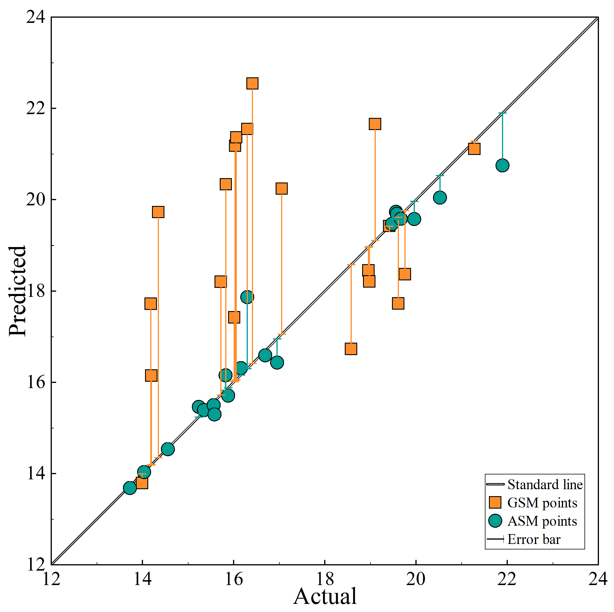
In order to compare the initial prediction accuracy of the global surrogate model (GSM) and the adaptive surrogate model (ASM), 525 DOE points were selected to build the GSM, and 25 DOE points belonging to the same sub-region were used to build the ASM based on the layout sub-region, and error analysis was performed for these two models. Taking the coefficient of determination (R${}^2$) and the relative root mean square error (RMSE) as the evaluation index, the comparison of the error analysis results is shown in

Table 4. Surrogate model error comparison.

Subsystem	Response	Approximate Method	GSM		ASM
			RMSE	R${}^2$	RMSE	R${}^2$
Statics	m	RSM	0.05	0.97	0.00	1.00
	$\lambda$		0.81	0.56	0.08	0.94
	$\sigma$		0.12	0.86	0.12	0.86
Dynamics	$\widehat{\sigma }$	RBF	0.70	0.00	0.14	0.84
	$\widehat{d}$		0.04	0.98	0.08	0.94
	f		0.16	0.78	0.02	0.99

, and the fitting error of the maximum dynamic stress response $\widehat{\sigma }$, which is the most difficult to predict, is given in Figure 12. Obviously, the ASM has significant advantages in prediction accuracy.

The weights ${\omega }_{\mathrm{stat}}$ and ${\omega }_{\mathrm{dyna}}$ in the optimization objective function of Equation (3) are both chosen to be 0.5, and the denominator $m^{\left(0\right)}$ and ${\widehat{\sigma }}^{\left(0\right)}$ are chosen to be 1.4 kg and 20.0 MPa, respectively, which are taken from the median of DOE. Since the sequential method used as a comparison does not consider dynamics optimization, the coupling of statics and dynamics is performed in the specific implementation. The optimization results are shown in

Table 5. Optimization results.

Type	Symbols	Case 1		Case 2		Case 3		Sequential 1
		Initial	Optimum	Initial	Optimum	Initial	Optimum	Optimum
Variables	N	3	4	5	5	6	4	6
	T	1	4	3	4	5	4	2
	$b_{\mathrm{w}}$ (mm)	30.000	29.870	25.000	24.570	30.000	29.932	29.977
	$b_{\mathrm{f}}$ (mm)	18.000	17.990	12.000	11.840	18.000	12.120	17.982
	$t_{\mathrm{w}}$ (mm)	2.000	1.397	2.000	1.570	1.400	1.938	1.371
	$t_{\mathrm{f}}$ (mm)	2.000	0.783	2.000	1.380	1.400	0.830	0.779
	$t_{\mathrm{s}}$ (mm)	2.000	1.980	2.000	1.850	1.400	1.940	1.373
Responses	m (kg)	1.743	1.739	2.219	1.744	2.382	1.788	1.621
	$\sigma$ (MPa)	71.920	68.100	69.836	70.540	99.810	69.467	96.346
	$\lambda$	0.711	1.020 *	1.669	1.006 *	2.080	1.017 *	1.009 *
	$\widehat{d}$ (mm)	0.880	0.502 *	0.420	0.448	0.190	0.501 *	0.412
	$\widehat{\sigma }$ (MPa)	38.599	18.553	20.590	18.442	12.921	18.268	30.235
	f (Hz)	132.754	192.460	188.332	179.913 *	273.599	192.914	179.872 *
W2		3.175	2.170	2.615	2.168	2.347	2.191	2.670
System Iterations		13		16		18		89 3
Run time 4		2 h 23 m		2 h 56 m		2 h 09 m		5h 42 m

¹ Sequential optimization method as a comparison with the same starting point as Case 1; ² weighting objective function; ³ sequential iterations; ⁴ including analysis time of DOE points; * active constraint.

. Since it is a multi-objective optimization, the linearly weighted normalization function W is the most important objective to focus on. As can be seen, Cases 1 to 3 converged from different initial points to almost the same W. However, since the structural layout optimization problem is not a simple convex problem, it is almost impossible to have a globally optimal solution, so even though the objective function values W of the three cases are close, the design variables are different, especially for Case 2, even the optimal layout is different from the other two cases.

Compared with the sequential optimization method, the CSRC method is far ahead not only in terms of optimal results but also in terms of optimization efficiency. It should be noted that the run time includes the analysis time of DOE points, and since the sequential method involves a large number of DOE points to build a GSM, which consumes much time. On the contrary, the CSRC method uses the ASM, which does not require many initial points, but uses the results of each sub-region coordination to update the surrogate model, and the closer to the optimal point, the higher the prediction accuracy, thus saving significant run time. In addition, ASM is not the only reason for time saving; the role of optimized concurrency is more critical. While each optimization in sequential optimization needs to wait for the completion of the previous optimization level, this is not the case with concurrent optimization, where sub-region optimizations can be performed simultaneously so that the advantages of modern high-performance computers can be taken advantage of.

The optimization iteration histories for the four cases are given in Figure 13, which contains the percentage contribution of the normalized mass m and the normalized RMS of maximum dynamic stress response $\widehat{\sigma }$ to the total weighted objective function. It can be seen that the CSRC method converges to almost the same percentage contribution because the collaborative interaction between disciplines allows some disciplines to discard their own optimums and pursue the global optimum, thus broadening the scope of the optimal search. Case 3 is an apparent example, which can be seen in Table 5, where the dynamics optimization result is even higher than the initial value, but the overall optimization results are optimal. In contrast, disciplinary coupling in sequential optimization leads to interdisciplinary constraints, with each discipline pursuing only its own optimal solution, thus narrowing the optimization search space.

6. Conclusions

In this paper, a new method was proposed for the static–dynamic coupled layout optimization problem of stiffened plates. The basic idea of this method is derived from the CO method of MDO, where the original problem is decomposed into multiple sub-region problems by decoupling the disciplines and variables separately, the connection between variables is ensured by sub-region coordination, and the disciplines are maintained by system-level optimization and consistency constraints, with each sub-region optimizaiton being able to perform concurrently. Furthermore, additional work for this paper was as follows:

• In order to improve the problem of slow convergence of the original CO algorithm in the feasible region, a dynamic driving function was added, and a numerical example was used to demonstrate the higher stability and efficiency of the CO algorithm with the addition of the dynamic driving function;
• Since the CO algorithm suffered from the ill-conditioned problem of the KKT stationary condition at the optimum point, the continuous sub-region optimization was carried out with the surrogate model. However, the abrupt change in discrete variables will lead to a decrease in the accuracy of the surrogate model. Thus, according to the special form of sub-region coordination, an adaptive surrogate model was proposed so that the results of each round of sub-region coordination can be used for the update of the surrogate model, and the closer to the optimal point, the higher the accuracy of the ASM;
• The proposed CSRC method was applied to an example of a static–dynamic coupled layout optimization problem of the stiffened plate, and three initial point cases, as well as a sequential approach case, were selected for comparison.

The application result showed that the three initial point cases converged to almost the same optimal objective function, even though the optimal design variables differed due to the nonconvexity of the layout optimization problem, demonstrating the robustness of the CSRC method. Furthermore, by utilizing the collaboration between disciplines, the CSRC method expanded the optimization search space to the extent that better result than the coupled sequential optimization method was obtained. In addition, the run time was considerably reduced by the application of the adaptive agent model and the concurrent nature of sub-region optimization.

As mentioned in the introduction of this paper, the idea of truss structure layout optimization has spawned the development of other structural layout optimizations. It is believed that the potential of the CSRC method for disciplines’ coupled layout optimization problems can be extended to more structural applications as well.

References

1. Duan, B.Y.; Ye, S.H. A mixed method for shape optimization of skeletal structures. Eng. Optimiz. 1986, 10, 183–197. [Google Scholar] [CrossRef]
2. Gholizadeh, S. Layout optimization of truss structures by hybridizing cellular automata and particle swarm optimization. Comput. Struct. 2013, 125, 86–99. [Google Scholar] [CrossRef]
3. Azid, I.A.; Kwan, A.S.K.; Seetharamu, K.N. An evolutionary approach for layout optimization of a three-dimensional truss. Struct. Multidiscip. Optim. 2002, 24, 333–337. [Google Scholar] [CrossRef]
4. Carvalho, J.P.G.; Lemonge, A.C.C.; Hallak, P.H.; Vargas, D.E.C. Simultaneous sizing, shape, and layout optimization and automatic member grouping of dome structures. Structures 2020, 28, 2188–2202. [Google Scholar] [CrossRef]
5. Vanderplaats, G.N.; Moses, F. Automated design of trusses for optimum geometry. J. Struct. Div. 1972, 98, 671–690. [Google Scholar] [CrossRef]
6. Kripakaran, P.; Gupta, A.; Baugh, J.W. A novel optimization approach for minimum cost design of trusses. Comput. Struct. 2007, 85, 1782–1794. [Google Scholar] [CrossRef]
7. Flager, F.; Adya, A.; Haymaker, J.; Fischer, M. A bi-level hierarchical method for shape and member sizing optimization of steel truss structures. Comput. Struct. 2014, 131, 1–11. [Google Scholar] [CrossRef]
8. Feng, Y.L.; Chen, J.L.; Yao, W.X. Concurrent subspace optimum design method for composite stiffened panel. J. Nanjing Univ. Aeronaut. Astronaut. 2013, 45, 360–366. (In Chinese) [Google Scholar]
9. Wang, B.; Hao, P.; Li, G.; Tian, K.; Du, K.F.; Wang, X.J.; Zhang, X.; Tang, X.H. Two-stage size-layout optimization of axially compressed stiffened panels. Struct. Multidiscip. Optim. 2014, 50, 313–327. [Google Scholar] [CrossRef]
10. Liu, W.L.; Butler, R.; Kim, H.A. Optimization of composite stiffened panels subject to compression and lateral pressure using a bi-level approach. Struct. Multidiscip. Optim. 2008, 36, 235–245. [Google Scholar] [CrossRef] [Green Version]
11. An, H.C.; Chen, S.Y.; Huang, H. Multi-objective optimization of a composite stiffened panel for hybrid design of stiffener layout and laminate stacking sequence. Struct. Multidiscip. Optim. 2018, 57, 1411–1426. [Google Scholar] [CrossRef]
12. Putra, G.L.; Kitamura, M.; Takezawa, A. Structural optimization of stiffener layout for stiffened plate using hybrid ga. Int. J. Nav. Arch. Ocean. 2019, 11, 809–818. [Google Scholar] [CrossRef]
13. Vanderplaats, G.N. Structural optimization for statics, dynamics and beyond. J. Braz. Soc. Mech. Sci. 2006, 28, 316–322. [Google Scholar] [CrossRef] [Green Version]
14. Sobieszczanski-Sobieski, J. A Linear Decomposition Method for Large Optimization Problems: Blueprint for Development; Technical Report NASA-TM-83248; NASA: Washington, DC, USA, 1982. Available online: https://ntrs.nasa.gov/citations/19820014371 (accessed on 15 March 2022).
15. Sobieszczanski-Sobieski, J. Optimization by Decomposition: A Step from Hierarchic to Non-Hierarchic Systems; Technical Report NASA-TM-101494; NASA: Washington, DC, USA, 1988. Available online: https://ntrs.nasa.gov/citations/19890004052 (accessed on 16 March 2022).
16. Kroo, I.; Altus, S.; Braun, R.; Gage, P.; Sobieski, I. Multidisciplinary optimization methods for aircraft preliminary design. In Proceedings of the 5th Symposium on Multidisciplinary Analysis and Optimization, AIAA, Panama City Beach, FL, USA, 7–9 September 1994. [Google Scholar] [CrossRef] [Green Version]
17. Sobieszczanski-Sobieski, J.; Agte, J.S.; Sandusky, R.R. Bi-level integrated system synthesis (bliss). In Proceedings of the 7th AIAA/USAF/NASA/ISSMO Symposium on Multidisciplinary Analysis and Optimization AIAA, St. Louis, MO, USA, 2–4 September 1998; p. 4916. [Google Scholar] [CrossRef] [Green Version]
18. Altus, T.D.; Sobieszczanski-Sobieski, J. A Response Surface Methodology for Bi-Level Integrated System Synthesis (Bliss); Technical Report NASA/CR-2002-211652; NASA: Washington, DC, USA, 2002. Available online: https://ntrs.nasa.gov/citations/20020063599 (accessed on 15 May 2022).
19. Fu, S.Y.; Huang, H.Y.; Lin, Z.X. Collaborative optimization of container ship on static and dynamic responses. Procedia Eng. 2012, 31, 613–621. [Google Scholar] [CrossRef]
20. Wang, W.W.; Gao, F.L.; Cheng, Y.T.; Lin, C. Multidisciplinary design optimization for front structure of an electric car body-in-white based on improved collaborative optimization method. Int. J. Auto. Technol. 2017, 18, 1007–1015. [Google Scholar] [CrossRef]
21. Qian, Y.; Wang, D. Optimization design of ship engine room structures based on sectionalized dynamic relaxation collaborative optimization method. Chin. J. Ship Res. 2016, 11, 40–46. (In Chinese) [Google Scholar]
22. Alexandrov, N.M.; Lewis, R.M. Analytical and computational aspects of collaborative optimization for multidisciplinary design. AIAA J. 2002, 40, 301–309. [Google Scholar] [CrossRef]
23. Parashar, S.; Bloebaum, C.L. Decision support tool for multidisciplinary design optimization (mdo) using multi-domain decomposition. In Proceedings of the 46th AIAA/ASME/ASCE/AHS/ASC Structures, Structural Dynamics and Materials Conference, AIAA, Austin, TX, USA, 18–21 April 2005. [Google Scholar] [CrossRef]
24. Braun, R.; Gage, P.; Kroo, I.; Sobieski, I. Implementation and performance issues in collaborative optimization. In Proceedings of the 6th Symposium on Multidisciplinary Analysis and Optimization, AIAA, Bellevue, WA, USA, 4–6 September 1996; p. 4017. [Google Scholar] [CrossRef] [Green Version]
25. Murphy, A.; Quinn, D.Q.; Mawhinney, P.; Özakca, M.; van der Veen, S. Tailoring static strength performance of metallic stiffened panels by selective local sub-stiffening. In Proceedings of the 47th AIAA/ASME/ASCE/AHS/ASC Structures, Structural Dynamics, and Materials Conference, AIAA, Newport, RI, USA, 1–4 May 2006. [Google Scholar] [CrossRef]
26. Sun, Z.B.; Ge, M.M.; Wang, Y.Y.; Wang, H.Q. Two-Level Layout Optimization Method for Metal Stiffened Thin-Walled Cone. J. Nanjing Univ. Aeronaut. Astronaut. 2015, 47, 566–570. (In Chinese) [Google Scholar] [CrossRef]
Figure 1. Schematic of metal stiffened plate.
Aerospace 10 00263 g001
Figure 2. Section types of stiffeners.
Aerospace 10 00263 g002
Figure 3. Flowchart of CSRC framework.
Aerospace 10 00263 g003
Figure 4. Schematic of semi-orthogonal values of sub-region coordination.
Aerospace 10 00263 g004
Figure 5. Interaction logic of ASM.
Aerospace 10 00263 g005
Figure 6. Data distribution of adaptive surrogate model (a) Initial surrogate model (by optimal latin hypercube); (b) Updated surrogate model (by sub-region adaptation).
Aerospace 10 00263 g006
Figure 7. Numerical test iteration path (a) Relaxation CO method; (b) Relaxation CO method with DDF.
Aerospace 10 00263 g007
Figure 8. Schematic of CO method process (a) Initial point in the infeasible zone; (b) Initial point in the feasible zone.
Aerospace 10 00263 g008
Figure 9. Initial geometry model of Case 1.
Aerospace 10 00263 g009
Figure 10. Load cases of stiffened plate.
Aerospace 10 00263 g010
Figure 11. Random vibration acceleration excitation.
Aerospace 10 00263 g011
Figure 12. Comparison of σ ^ error between GSM and ASM.
Aerospace 10 00263 g012
Figure 13. Optimization iteration history (a) Case 1; (b) Case 2; (c) Case 3; (d) Sequential case.
Aerospace 10 00263 g013