Radial Basis Function Model-Based Adaptive Model Predictive Control for Trajectory Tracking of a Clapping-Wing Micro Air Vehicle

Abstract

Clapping-wing micro air vehicles (CWMAVs) face many control problems due to their lightweight design and susceptibility to disturbances. This study proposes a radial basis function (RBF) model-based adaptive model predictive control (AMPC) for trajectory tracking to solve the control problem in the presence of internal uncertainties and external disturbances. First, a method for calculating the desired attitude is given. Second, a control optimization model is used by adjusting future control inputs to minimize the difference between the future and desired outputs. Third, a nonlinear predictive linearization is used to transform the nonlinear optimization model into a quadratic programming problem. Two observers are introduced to estimate the internal uncertainties and the external disturbances. Finally, the control assignment method is combined with the trajectory tracking method to obtain the design variables of actuators (flapping frequency, pitch angle, and yaw angle). Validation studies were performed to verify the effectiveness and accuracy in the presence of constant and time-dependent disturbances. The comparison of RAMPC with classical methods shows that RAMPC has better control performance with smaller errors. The proposed RAMPC framework can be well used for CWMAV control and provides an excellent basis for accurate navigation and autonomous obstacle avoidance.

1. Introduction

Micro air vehicles (MAVs) were proposed by the US Defense Advanced Research Projects Agency (DARPA) in 1992 [1,2] and were expected to become a new generation of military weapons in the future. Compared to the conventional propulsion systems of MAVs, the interest in flapping flight has increased in recent years due to the rapid development of mechanics and measurement technology in biology and aerospace science [3,4]. Observations of the natural flapping flight of birds and insects have provided tremendous inspiration for the development of MAVs in aeronautics. Flapping-wing micro air vehicles (FWMAVs), especially clapping-wing micro air vehicles with a double clap-fling mechanism, combine the advantages of fixed wing and rotor wing MAVs with better maneuverability, higher energy conversion rates, lower noise level, better concealment performance, and higher safety [5,6,7]. For the CWMAV, the realization of high-precision and high-stability flight control is the most important guarantee for its practical application. Although several CWMAV or FWMAV types exist, rare prototypes can realize an autonomous flight. Owing to the requirement for lightweight design, the size, weight, and power are limited, which leads to the degradation of the performance of sensors and actuators. These issues make CWMAV more susceptible to internal uncertainties and external disturbances, which place higher demands on control algorithms.

Numerous studies on the control algorithm of CWMAV have been conducted to meet these demands, mainly including PID, adaptive sliding mode control, linear quadratic regulator, model predictive control, etc.

Owing to difficulties in modeling MAVs with flapping wings, the control system of the mainstream prototype still uses the PID algorithm, a model-free algorithm [8] that works well for simple control tasks with low precision requirements. Verboom et al. [9] employed three independent PID controllers to control the flapping frequency, yaw tail angle, and pitch tail angle and realized the hovering flight of the FWMAV.

Modern state-space control methods can be more flexible and accurate when compared to PID control methods, especially in controlling complex nonlinear and time-dependent systems [10]. Among state-space control methods, the adaptive sliding mode control has good adaptability in the face of modeling uncertainties and external disturbances and is capable of adjusting the controller parameters [11,12]. Banazadeh and Taymourtash [13] designed an adaptive sliding mode control algorithm for the attitude and position control of the FWMAV in uncertain environments. Based on the quasi-steady assumption, they developed the average theory to convert the time-varying system to a time-invariant system. Bluman et al. [14] used a second-order sliding-mode control method to realize the hovering control of CWMAVs in the longitudinal plane. In the non-optimal initial state, they introduced external gust disturbance into the control algorithm, whose validation was proved by the experiment of hovering state within seconds.

The linear quadratic regulator (LQR) is another state-space-based method for designing an optimal controller considering disturbances [15,16]. Deng et al. [17] established a three-degree-of-freedom linearization model under the hovering condition of the CWMAV and proposed a top-down three-layer control framework to simplify the flight control design. Meanwhile, they designed a robust output feedback controller based on linear quadratic regulation, which only needs to pass sensor data to achieve a stable hovering flight by a simple affine transformation. Kim et al. [18] developed an aerodynamic model that considered the interaction of the leading vortices on the wing and tail. The LQR method was adopted to calculate the optimal control gain matrix at each flight speed. Simulation experiments show that their proposed control method can not only achieve the hovering flight of the CWMAV but also control the flight speed well.

Previous studies have primarily focused on the CWMAV control problem. However, they are not robust or efficient enough in the face of real-world uncertainties such as wind. In contrast to the aforementioned advanced control algorithms, model predictive control (MPC) emphasizes the function of the model and does not consider the internal structure of the model. MPC is an advanced control algorithm that has been successfully applied in the field of engineering control [19,20]. It calculates the control input by line optimization. The basic principle is to first measure the output and system state at a given time and use the system model to predict the system output in the future, and then calculate the optimal control input at the current time by minimizing the difference between the predicted output and the desired output. Its rolling optimization strategy can adapt well to the trajectory tracking system with internal uncertainties and external disturbances. Dutta and Das [21] proposed an explicit nonlinear predictive control technique model using multiple estimation models with a convex combination framework for a class of nonlinear MIMO systems. Yao et al. [22] presented the MPC strategy for building dynamic systems, which are generally nonlinear. They presented different challenges for its optimized control of energy-saving and thermal comfort. Zhu et al. [23] proposed the MPC scheme for a three-degrees-of-freedom flapping-wing unmanned air vehicle (UAV) to track the reference set point. In addition, the adaptive MPC extends the standard MPC by adapting the prediction model and controller parameters online in real-time to account for system changes; however, it is often cited only for MAVs with rotor wings.

A review of the literature indicates that the research considering internal uncertainties and external disturbances for MAVs with flapping wings, and especially for MAVs with clapping wings, is rarely included. Conversely, the mapping relationship between the dynamic model and actuator parameters in the control assignment module is often ignored, causing an incomplete closed-loop control. Therefore, a trajectory control model combining control assignment and adaptive model predictive control for CWMAVs is a research gap that motivated this study.

The novelty of the study is threefold: (1) a model predictive control framework for trajectory tracking of CWMAVs, based on the system state transition equation and three desired Euler angles; (2) an adaptively predictive control model with two observers to estimate internal uncertainties and external disturbances; and (3) a radial basis function model-based control assignment strategy to obtain the actuator control outputs of CWMAVs.

The remaining sections of this paper are organized as follows: Section 2 describes a radial basis function model-based adaptive model predictive control model of the CWMAV, considering internal uncertainties and external disturbances. Section 3 presents the tracking results of validation studies and discussions about accuracy. Section 4 presents the conclusion and recommendations for future studies.

2. Methodology

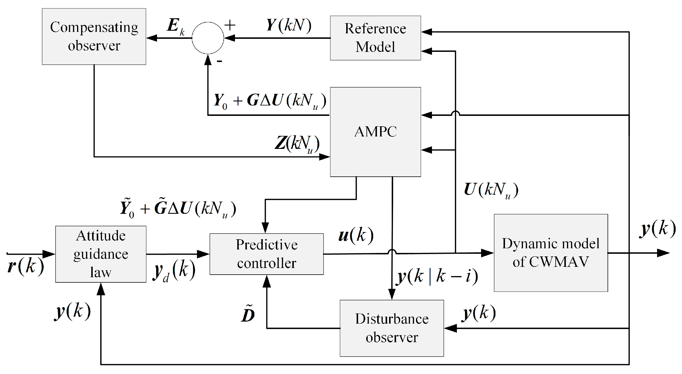
Uncertainties are considered in the proposed RAMPC framework. The procedure can be summarized as follows.

Step 1: Construct the system state transition equation $\dot{\mathit{V}}, \dot{\mathit{\omega }}$ at the time step $k$ to evaluate the current system state of the CWMAV.

Step 2: Evaluate the desired attitude angle $\varphi , \theta , \psi$ using the equation for the desired trajectory and the current flight state of the CWMAV. This ensures the real-time adjustment of the attitude angle during the trajectory tracking process.

Step 3: Calculate the future system vector that is based on the current system state and system measurement.

Step 4: Minimize the difference $J_s(k)$ between the future system vector and the desired vector using system incremental gain.

Step 5: Transfer the nonlinear trajectory tracking to linear quadratic programming.

Step 6: Design two observers to compensate for the system’s model uncertainties (internal uncertainties) and external disturbances.

Step 7: Obtain the AMPC output $\mathit{Y}(kN)$ at the time step $k$ and proceed to the time step $k+1$.

Step 8: Develop an aerodynamic radial basis function model based on the experimental data.

Step 9: Transfer the nonlinear control assignment to a constraint optimization problem to obtain the output evolution of actuators $\mathit{x}, \delta$.

The schematic diagram is shown in Figure 1, and the details will be introduced in the following sections.

2.1. Dynamic Modeling of CWMAV

2.1.1. Coordinate Definition

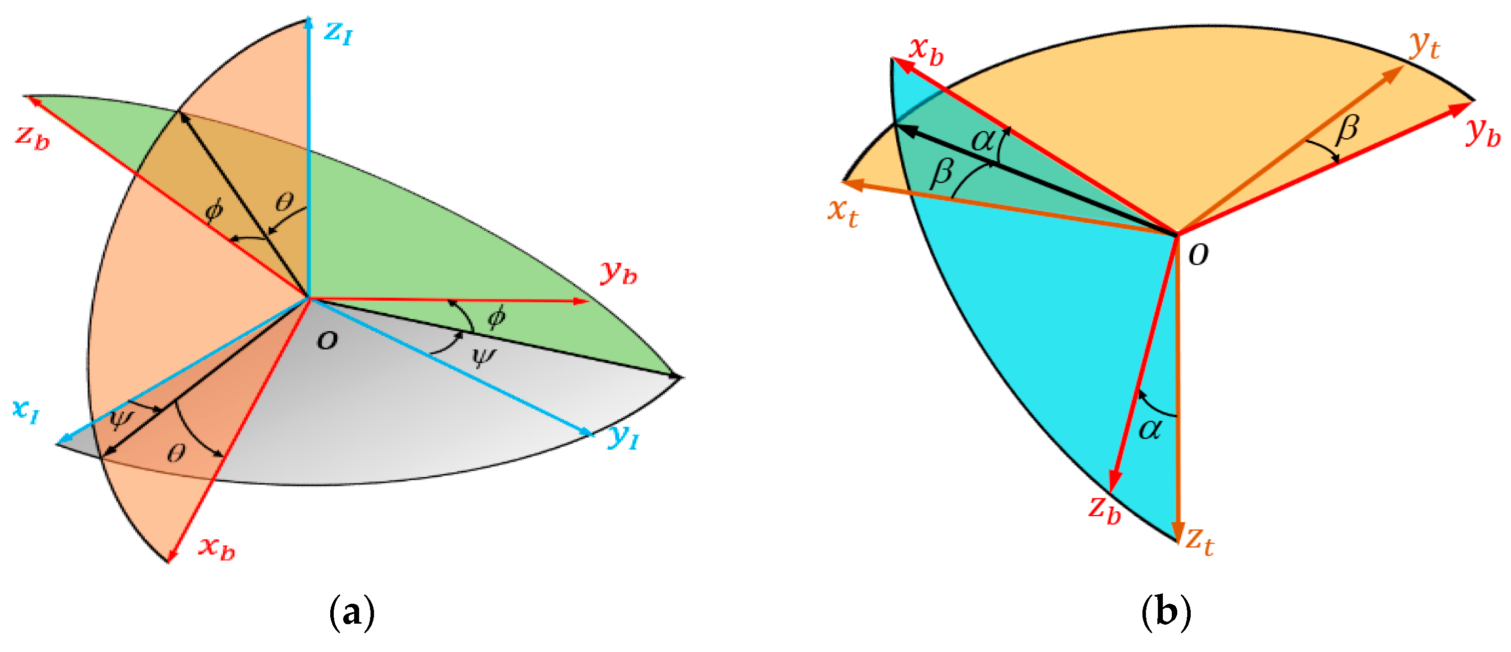
The inertial coordinate system can describe the absolute velocity and position of the CWMAV. The flight attitude and direction need to be defined by the body coordinate system and the track coordinate system, respectively. In Figure 2a, $\varphi$, $\theta$, $\psi$ are the Euler angles based on the angle between the body coordinate system and the inertial coordinate system. In Figure 2b, $o{x}_t$ represents the forward direction, where $\alpha$ and $\beta$ are the angle of attack and sideslip angle, respectively.

2.1.2. Nonlinear Dynamics System of CWMAV

According to the law of conservation of momentum, the force $F_b$ and torque $M_b$ in the body coordinate on the CWMAV can be expressed as:

$$\begin{array}{l}{F}_b=\frac{d}{dt}mV\\ M_b=\frac{d}{dt}I\omega \end{array}$$

(1)

where $m$ is the total mass of CWMAV.

$$\begin{array}{l}{F}_b{}^T={\left[\begin{array}{ccc}m\frac{du}{dt}& m\frac{dv}{dt}& m\frac{dw}{dt}\end{array}\right]}^T\\ I\omega =\left[\begin{array}{ccc}{I}_x& -I_{xy}& -I_{zx}\\ -I_{xy}& I_y& -I_{yz}\\ -I_{zx}& -I_{yz}& I_z\end{array}\right]\left[\begin{array}{c}p\\ q\\ r\end{array}\right]\end{array}$$

(2)

where $V=[u, v, w]$ are the velocity components for the three axes in the body coordinate system. $\omega =[p, q, r]$ are the components of angular velocity. $I_x, I_y, I_z$ are the moments of inertia. $I_{xz}, I_{xy}, I_{yz}$ are the products of inertia

The dynamic system of the CWMAV in the body coordinate system can be expressed as:

$$\begin{array}{l}F=F_b+m\left(\omega \times V\right)\\ M=M_b+\omega \times I\omega \end{array}$$

(3)

Considering the axisymmetric traits of CWMAV’s moment of inertia, $I_{xy}=I_{yz}=0$, the nonlinear dynamic equation of the system is introduced into the solver based on Equations (1)–(3), which can be written as follows:

$$\begin{array}{l}\dot{u}=\frac{F_x}{m}-g\sin \theta -wq+vr\\ \dot{v}=\frac{F_y}{m}-g\cos \theta \cos \varphi -ru+pw\\ \dot{w}=\frac{F_z}{m}-g\cos \theta \sin \varphi -pv+qu\end{array}$$

(4)

$$\begin{array}{l}\dot{p}=\frac{1}{I_x}\left(\left(I_y-I_z\right)qr+\left(\dot{r}+pq\right)I_{xz}+M_x\right)\hfill \\ \dot{q}=\frac{1}{I_y}\left(\left(I_z-I_x\right)pr+I_{xz}\left(r^2-p^2\right)+M_y\right)\hfill \\ \dot{r}=\frac{1}{I_z}\left(\left(I_x-I_y\right)pq+\left(I_{xz}\dot{p}-qr\right)+M_z\right)\hfill \end{array},$$

(5)

The position and orientation of the CWMAV in actual flight cannot be described by the body coordinate system. In order to determine the transformation matrix from the inertial coordinate system to the body coordinate system, the Euler angular rate ${[\dot{\varphi }, \dot{\theta }, \dot{\psi }]}^T$ needs to be calculated by the angular velocity component ${[p, q, r]}^T$.

$$\left[\begin{array}{c}\dot{\varphi }\\ \dot{\theta }\\ \dot{\psi }\end{array}\right]=\left[\begin{array}{ccc}1& \sin \varphi \tan \theta & \cos \varphi \tan \theta \\ 0& \cos \varphi & -\sin \varphi \\ 0& \sin \varphi \sec \theta & \cos \varphi \sec \theta \end{array}\right]\left[\begin{array}{l}p\hfill \\ q\hfill \\ r\hfill \end{array}\right],$$

(6)

Similarly, the absolute velocity component can be determined by the Euler angle ${[\varphi , \theta , \psi ]}^T$ and the velocity component ${[u,v,w]}^T$ in the body coordinates. The absolute velocity can be expressed as:

$$\left[\begin{array}{c}\frac{\mathrm{d}x}{ \mathrm{d}t}\\ \frac{\mathrm{d}y}{ \mathrm{d}t}\\ \frac{\mathrm{d}z}{ \mathrm{d}t}\end{array}\right]=R^{Ib}(\varphi ,\theta ,\psi )\left[\begin{array}{c}u\\ v\\ w\end{array}\right],$$

(7)

where

$$R^{Ib}={\left(R^{bI}\right)}^T=\left[\begin{array}{ccc}1& 0& 0\\ 0& \cos \varphi & \sin \varphi \\ 0& -\sin \varphi & \cos \varphi \end{array}\right]\left[\begin{array}{ccc}\cos \theta & 0& -\sin \theta \\ 0& 1& 0\\ \sin \theta & 0& \cos \theta \end{array}\right]\left[\begin{array}{ccc}\cos \psi & \sin \psi & 0\\ -\sin \psi & \cos \psi & 0\\ 0& 0& 1\end{array}\right],$$

(8)

There are several sources of uncertainties to be considered in flapping propulsion, including manufacturing errors, environmental disturbances, and morphological changes in the structure and wings during flapping flight. In addition, the CWMAV usually encounters unstable factors, such as low-altitude gusts. The design of the CWMAV usually focuses on lightweight construction and is made of non-metallic material. These design methods reduce the robustness of the CWMAV and increase the risk of failure. Therefore, considering the uncertainties and the disturbance, the internal uncertainties and external disturbance terms are parameterized and added to Equations (4) and (5). Then, the state equation of the system can be rewritten as follows:

$$\begin{array}{l}\dot{V}=\left(f+\Delta \mathit{f}\right)-\Omega \times V+{\mathit{D}}_v\\ \dot{\mathit{\omega }}={\mathit{I}}^{-1}\left(\mathit{M}+\Delta \mathit{M}\right)-{\mathit{I}}^{-1}\mathit{\Omega }\times \left(\mathit{I}\mathit{\omega }\right)+D_w\end{array}$$

(9)

where $\mathit{f}=\mathit{F}/m$ is the linear acceleration generated by the resultant external force. $\Omega$ is the obliquely symmetric matrix of angular velocity; $\Delta \mathit{f}$ and $\Delta \mathit{M}$ are the uncertain parts of line acceleration and angular acceleration; $D_v$ and $D_{\omega }$ are the external disturbances in the translational and rotational flights.

The system state transition equation is performed to realize the trajectory tracking control of the CWMAV, and the inputs $u$ and outputs $y$ of the system are defined as follows:

$$\begin{array}{l}u={\left[\begin{array}{cccccc}{F}_x& F_y& F_z& M_x& M_y& M_z\end{array}\right]}^{\mathrm{T}}\\ y={\left[\begin{array}{cccccc}x& y& z& \varphi & \theta & \psi \end{array}\right]}^{\mathrm{T}}\end{array}$$

(10)

where $\left[\begin{array}{cccccc}{F}_x& F_y& F_z& M_x& M_y& M_z\end{array}\right]$ are the force and moment of the CWMAV in the body coordinate system. $x, y, z$ are the position coordinate components in the inertial coordinate system.

In addition, the desired velocity and angular velocity components are tracked to achieve a better control effect [24]. Therefore, the entire system output is rewritten as follows:

$$y={\left[\begin{array}{cccccccccccc}x& y& z& \dot{x}& \dot{y}& \dot{z}& \varphi & \theta & \psi & \dot{\varphi }& \dot{\theta }& \dot{\psi }\end{array}\right]}^{\mathrm{T}},$$

(11)

2.1.3. Desired System State Solving

For the trajectory tracking problem, the input of the system is generally the equation of motion of the desired trajectory, and the attitude motion equation of the CWMAV is not specified. The attitude angle of the CWMAV tremendously influences its aerodynamic performance, so the desired attitude angle (including roll, yaw, and pitch angles) is well calculated in this study, based on the desired trajectory equation and actual flight state of the CWMAV.

In order to estimate the desired roll angle, the force analysis in the body coordinate system $o{z}_b{y}_b$ is shown in Figure 3, where $F_{ef}^{}$ is the centripetal force and ${\varphi }_d$ is the desired roll angle. Due to the limited lateral aerodynamic capabilities of the CWMAV, the centripetal force $F_{ef}$ during the steering motion is mainly generated by the centripetal component of aerodynamic lift. During the roll motion, the yaw moment is created by the vertical tail, which generates a sideslip angle so that the wings have a lift difference for this roll motion. Since the lateral force generated by the tail is small compared to the wings, it is assumed that the centripetal force and gravity are provided by the normal aerodynamic force. Then, the desired roll angle can be expressed as follows:

$${\varphi }_d(k+1)=\arctan (\frac{\dot{x}{(k)}^2+\dot{y}{(k)}^2}{r(k)g}),$$

(12)

where $r(k)$ is the curvature radius at the actual flight position of the aircraft at time k, and $\dot{x}(k), \dot{y}(k)$ are the velocities in the inertial coordinate system at time k.

In order to calculate the desired yaw angle, the force analysis is shown in Figure 4a in the inertial coordinate system. In Figure 4a, $x(k), y(k), z(k)$ are the positions at time k. According to the measurement results of the wind tunnel experiment, the sideslip angle during actual flight is particularly small due to the weak lateral aerodynamic performance of the CWMAV. Based on the difference between the actual position and the desired position in the inertial coordinate system, the desired yaw angle in the next time step can be expressed as follows:

$${\psi }_d(k+1)=\arctan \left(\frac{y(k+1)-y(k)}{x(k+1)-x(k)}\right),$$

(13)

The force analysis in the inertial coordinate system to estimate the desired pitch angle is shown in Figure 4b. The angle of attack during flight cannot be ignored for the CWMAV. Therefore, the desired pitch angle ${\theta }_d(k+1)$ should be expressed by the sum of the desired track angle and the angle of attack:

$${\theta }_d(k+1)=\alpha (k)+\arctan \left(\frac{z(k+1)-z(k)}{\sqrt{x_{}^2(k+1)+y_{}^2(k+1)}-\sqrt{x_{}^2(k)+y_{}^2(k)}}\right),$$

(14)

where $\alpha (k)$ is the angle of attack at time k.

2.2. Adaptive Model Predictive Control for Trajectory Tracking of CWMAV

2.2.1. MPC Trajectory Tracking Controller for CWMAV

In order to obtain the control variable of the system in the MPC framework, an optimization problem must be solved in each prediction time domain. By adjusting the future control input to minimize the difference between the future output and the desired output, the optimization problem in the prediction time domain can be expressed as follows:

$$\begin{array}{l}\underset{\Delta \mathit{u}}{\min } J_s(k)={\displaystyle {\displaystyle \sum }_{j=1}^N}\parallel y(k+j|k)-y_d(k+j){\parallel }_{\mathit{Q}}^2+{\displaystyle {\displaystyle \sum }_{j=0}^{N_u}}\parallel \Delta u(k+j|k){\parallel }_{\mathit{R}}^2\\ \mathrm{s}.\mathrm{t}. \\ \hspace{1em}\hspace{1em}\hspace{1em}\hspace{1em}\Delta u_{\min }<\Delta u(k+j)<\Delta u_{\max },\hspace{1em}0\le j\le N_u\\ \hspace{1em}\hspace{1em}\hspace{1em}\hspace{1em}{u}_{\min }<u(k+j)<u_{\max },\hspace{1em}0\le j\le N_u\\ \hspace{1em}\hspace{1em}\hspace{1em}\hspace{1em}y(k+N+1|k)=y_d(k+N+1)\end{array}$$

(15)

where $\mathit{y}(k+j|k)$ represents the predicted output at time $k+j$ based on time $k$; ${\mathit{y}}_d(k+j)$ is the desired out time at $k+j$; $\mathit{u}(k+j)$ and $\Delta \mathit{u}(k+j|k)$ are the system input and the increment of the system input at time $k+j$, respectively. $\mathit{Q}, \mathit{R}$ is the weighted diagonal matrix with the tracking error and the smooth control input, respectively, and $N, N_u$ are the time domains of the predicted output and the initial input. To increase the accuracy of the system tracking, $N>N_u$ is generally used to provide a larger time domain for the control system. ${\mathit{u}}_{\min }, {\mathit{u}}_{\max }$ and $\Delta {\mathit{u}}_{\min }, \Delta {\mathit{u}}_{\max }$ are the upper and lower boundaries of the control input and control input increment, respectively. $\mathit{y}(k+N+1|k)={\mathit{y}}_d(k+N+1)$ is the terminal constraint used to ensure the progressive stability of the closed-loop system.

In order to obtain the desired attitude angle at the current time, the relative position difference between the CWMAV location and the desired trajectory is calculated by Equations (12)–(14). The control quantity, system output, control increment, and control expectation in the same time window are expressed as follows:

$$\mathit{U}(k{N}_u)={\left[\begin{array}{cccc}\mathit{u}{(k)}^T& \mathit{u}{(k+1)}^T& \dots & \mathit{u}{(k+N_u)}^T\end{array}\right]}^T,$$

(16)

$$\Delta \mathit{U}(k{N}_u)={\left[\begin{array}{cccc}\Delta \mathit{u}{(k)}^T& \Delta \mathit{u}{(k+1)}^T& \dots & \Delta \mathit{u}{(k+N_u)}^T\end{array}\right]}^T,$$

(17)

$$\mathit{Y}(kN)={\left[\begin{array}{cccc}\mathit{y}{(k)}^T& \mathit{y}{(k+1)}^T& \dots & \mathit{y}{(k+N)}^T\end{array}\right]}^T,$$

(18)

$${\mathit{Y}}_d(kN)={\left[\begin{array}{cccc}{\mathit{y}}_d{(k)}^T& {\mathit{y}}_d{(k+1)}^T& \dots & {\mathit{y}}_d{(k+N)}^T\end{array}\right]}^T,$$

(19)

Then, the cost function of Equation (15) can be re-expressed as:

$$\begin{array}{l}{J}_s(k)={\left(\mathit{Y}(kN)-{\mathit{Y}}_d(kN)\right)}^{\mathrm{T}}\overline{\mathit{Q}}\left(\mathit{Y}(kN)-{\mathit{Y}}_d(kN)\right)\\ \hspace{1em}\hspace{1em}\hspace{1em}+\Delta \mathit{U}{(k{N}_u)}^T\overline{\mathit{R}}\Delta \mathit{U}(k{N}_u)\end{array}$$

(20)

$$\overline{\mathit{Q}}={\left[\begin{array}{ccc}\mathit{Q}& & 0\\ & \ddots & \\ 0& & \mathit{Q}\end{array}\right]}_{12N\times 12N}\overline{\mathit{R}}={\left[\begin{array}{ccc}\mathit{R}& & 0\\ & \ddots & \\ 0& & \mathit{R}\end{array}\right]}_{6(N_u+1)\times 6(N_u+1)},$$

(21)

where, $\overline{\mathit{Q}}\in {ℝ}^{12N\times 12N}, \overline{\mathit{R}}\in {ℝ}^{6(N_u+1)\times 6(N_u+1)}$ are the extended diagonal positive definite matrices for $\mathit{Q}$ and $\mathit{R}$, respectively.

Considering the nonlinear dynamic system of the CWMAV from Equations (4) and (5), the state equation of the input and output of the system is expressed as:

$$\dot{\mathit{y}}(t)=\mathit{h}(\mathit{y}(t),\mathit{u}(t)),$$

(22)

where $\mathit{h}$ is a nonlinear function by the dynamic equations of CWMAV. Then, the discretization of Equation (22) is expressed as follows:

$$\begin{array}{cc}\hfill \mathit{y}(k+i)& =\mathit{h}(\mathit{y}(k+i-1),\Delta \mathit{u}(k+i-1))\hfill \\ & =\mathit{h}(\mathit{h}(\mathit{y}(k+i-2),\Delta \mathit{u}(k+i-2)),\Delta \mathit{u}(k+i-1))\hfill \\ & =\dots \hfill \\ & ={\mathit{h}}_i(\mathit{y}(k),\Delta \mathit{U}(k(i-1))), 0\le i\le N\hfill \end{array}$$

(23)

The prediction output vector of the prediction time domain is obtained by Equations (18) and (23) as:

$$\begin{array}{cc}\hfill \mathit{Y}(kN)& ={[\mathit{h}(\mathit{y}(k)),\Delta \mathit{u}(k))}^T \dots {\mathit{h}}_N(\mathit{y}(k)),\Delta \mathit{U}(k(i-1)){)}^T{]}^T\hfill \\ & =\mathit{H}(\mathit{y}(k),\Delta \mathit{U}(kN))\hfill \end{array}$$

(24)

where the incremental control vector is expressed as:

$$\Delta \mathit{U}(kN)={\left[\Delta \mathit{U}{\left(k{N}_u\right)}^{\mathrm{T}} 0_{1\times 6\left(N-N_u\right)}\right]}^{\mathrm{T}},$$

(25)

From Equation (25), it can be seen that the proposed trajectory tracking controller becomes a nonlinear structure due to this nonlinear prediction model. In order to increase the efficiency of the traditional low-order Taylor expansion linearization method, a nonlinear predictive linearization (NPL) is proposed in [25] to approximate the nonlinear output, where $\mathit{Y}(kN)$ can be represented as a linear combination of the control increments:

$$\begin{array}{l}\mathit{Y}(kN)={\mathit{Y}}_0+\mathit{G}(k{N}_u)\Delta \mathit{U}(k{N}_u)\\ {\mathit{Y}}_0=\mathit{H}(\mathit{y}(k),0)\end{array}$$

(26)

where ${\mathit{Y}}_0$ is the steady-state output trajectory when the system input is unchanged and $\mathit{G}$ is the step response coefficient matrix of each input corresponding to the output:

$$\mathit{G}=\left[\begin{array}{cccc}{s}_1(k{N}_u)& 0& \dots & 0\\ s_2(k{N}_u)& s_1(k{N}_u)& \cdots & 0\\ ⋮& ⋮& \ddots & ⋮\\ s_N(k{N}_u)& s_{N-1}(k{N}_u)& \cdots & s_{N-N_u+1}(k{N}_u)\end{array}\right],$$

(27)

where $s(k{N}_u)$ is the step response coefficient.

Finally, the cost function of Equation (20) can be rewritten as:

$$J_s(k)={\Vert {\mathit{Y}}_0+\mathit{G}\Delta \mathit{U}(k{N}_u)-{\mathit{Y}}_d(kN)\Vert }_{\overline{\mathit{Q}}}^2+{\Vert \Delta \mathit{U}(kN)\Vert }_{\overline{\mathit{R}}}^2,$$

(28)

The solution to the trajectory tracking control problem is transformed into a quadratic programming problem, which can be used to solve the system input quickly by a linear controller.

2.2.2. Adaptive Model Predictive Control Model of CWMAV

As mentioned earlier about the MPC framework of the CWMAV, this section discusses the model parameter’s uncertainty and external disturbances to perform adaptive model prediction control (AMPC).

AMPC Model for CWMAV

The prediction vector in AMPC can be defined as follows:

$$\mathit{Y}(kN)={\mathit{Y}}_0+\Delta {\mathit{Y}}_0+(\mathit{G}+\Delta \mathit{G})\Delta \mathit{U}\left(k{N}_u\right)+{\mathit{D}}_e,$$

(29)

where $\Delta {\mathit{Y}}_0$ and $\Delta \mathit{G}$ are the uncertain inputs of the system model, ${\mathit{D}}_e$ is the high-order nonlinear input of the external disturbance, and the total disturbance is $\mathit{D}=\Delta {\mathit{Y}}_0+{\mathit{D}}_e$. It is worth noting that all model uncertainties and external disturbances are bounded in this study. The optimization model of Equation (20) can be transferred to:

$$\begin{array}{l}\underset{\Delta \mathit{U}}{\min }{J}_s(k)=\parallel {\mathit{Y}}_0+(\mathit{G}+\Delta \mathit{G})\Delta \mathit{U}+\mathit{D}-{\mathit{Y}}_d{\parallel }_{\overline{\mathit{Q}}}^2+\parallel \Delta \mathit{U}{\parallel }_{\overline{\mathit{R}}}^2\\ \mathrm{s}.\mathrm{t}. \\ \hspace{1em}\hspace{1em}\hspace{1em}\hspace{1em}\Delta {\mathit{u}}_{\min }<\Delta \mathit{u}(k+j)<\Delta {\mathit{u}}_{\max },\hspace{1em}0\le j\le N_u\\ \hspace{1em}\hspace{1em}\hspace{1em}\hspace{1em}{\mathit{u}}_{\min }<\mathit{u}(k+j)<{\mathit{u}}_{\max },\hspace{1em}0\le j\le N_u\\ \hspace{1em}\hspace{1em}\hspace{1em}\hspace{1em}\Vert \mathit{D}\Vert \le D_{\max }\\ \hspace{1em}\hspace{1em}\hspace{1em}\hspace{1em}\Vert \Delta \mathit{G}\Vert \le \Delta G_{\max }\\ \hspace{1em}\hspace{1em}\hspace{1em}\hspace{1em}\mathit{y}(k+N+1\mid k)={\mathit{y}}_d(k+N+1)\end{array}$$

(30)

where $D_{\max }, \Delta G_{\max }$ are the maximum values of disturbances and uncertainties, respectively.

Since the disturbances and uncertainty boundaries cannot be easily estimated, two observers were developed in this study to compensate for the system’s model uncertainties and external disturbances.

Designing of the Compensation Observer

In order to transform the optimization problem into a quadratic programming problem, a compensation observer is introduced to compensate for the uncertainty of the system, and the error $\mathit{E}$ between the actual output and the predicted output of the system is defined as:

$${\mathit{E}}_k=\mathit{Y}(kN)-{\mathit{Y}}_0-\mathit{G}\Delta \mathit{U}(k{N}_u)={\mathit{Z}}_k^T{\mathit{X}}_k,$$

(31)

where ${\mathit{Z}}_k^{}={[\Delta \hat{\mathit{G}}\hat{\mathit{D}}]}^T$, ${\mathit{X}}_k={[\Delta \mathit{U}(k{N}_u)1]}^T$. $\Delta \hat{\mathit{G}}$ and $\hat{\mathit{D}}$ are the estimated values of internal uncertainty and external disturbance, respectively. The error vector can be expressed by collecting $N_u+1$ input and output data in the prediction time domain as follows:

$$\left[\begin{array}{cccc}{\mathit{E}}_i& {\mathit{E}}_{i+1}& \dots & {\mathit{E}}_{i+N_u}\end{array}\right]={\mathit{Z}}_{i+N_u+1}^{\mathrm{T}}\left[\begin{array}{cccc}{\mathit{X}}_i& {\mathit{X}}_{i+1}& \dots & {\mathit{X}}_{i+N_u}\end{array}\right],$$

(32)

$${\mathit{Z}}_{i+N_u+1}^{\mathrm{T}}=\left[\begin{array}{cccc}{\mathit{E}}_i& {\mathit{E}}_{i+1}& \dots & {\mathit{E}}_{i+N_u}\end{array}\right]{\left[\begin{array}{cccc}{\mathit{X}}_i& {\mathit{X}}_{i+1}& \dots & {\mathit{X}}_{i+N_u}\end{array}\right]}^{-1},$$

(33)

$\Delta \mathit{G}$ and $D$ can be inversely solved using ${\mathit{E}}_k$ and ${\mathit{X}}_k$ at each time step by Equation (31) to ensure that the error of the model is zero at time step $N+1$. In order to reduce the computational cost of the proposed model, the least mean square (LMS) algorithm is used instead of the inverse matrix solver in Equation (34).

$${\mathit{Z}}_{i+1}={\mathit{Z}}_i+\gamma ({\mathit{E}}_i-{\mathit{Z}}_i^T{\mathit{X}}_i){\mathit{X}}_i^T,$$

(34)

where $\gamma$ is the searching step length. The convergence study of this search algorithm can be found in [26]. Then, using the uncertainty compensation observer, Equation (24) can be modified by this uncertainty compensation observer as follows:

$$\mathit{Y}(kN)={\tilde{\mathit{Y}}}_0+\tilde{\mathit{G}}\Delta \mathit{U}(k{N}_u),$$

(35)

where

$$\begin{array}{l}{\tilde{\mathit{Y}}}_0={\mathit{Y}}_0+\hat{\mathit{D}}\\ \tilde{\mathit{G}}=\mathit{G}+\Delta \hat{\mathit{G}}\end{array}$$

(36)

where ${\tilde{\mathit{Y}}}_0$ and $\tilde{\mathit{G}}$ are the modified steady-state output vector and step response output matrix, respectively.

Designing of the Disturbance Observer

External disturbances are another factor for the input error in this study. The entire prediction model can be expressed as follows:

$$\mathit{Y}(kN)={\mathit{Y}}_0+(\mathit{G}+\Delta \hat{\mathit{G}})\Delta \mathit{U}(kN)+\hat{\mathit{D}}+\tilde{\mathit{D}},$$

(37)

where $\tilde{\mathit{D}}$ is the higher-order disturbance term. A disturbance observer is proposed to estimate the difference between the predicted output and the actual output of the system.

In the classical MPC model, the disturbance term $d$ is generally assumed to be a constant over the entire prediction time window, i.e., $\mathit{d}(k+i|k)=\mathit{y}(k)-\mathit{y}(k|k-1)$, where $y(k)$ and $y(k|k-1)$ are the system output at time k and the predicted system output at time k, respectively. These models ignore the time-dependent disturbance, which easily leads to control errors. In this study, another observer—disturbance observer—is used, where the predicted disturbance is obtained from the previous output history. Therefore, the total disturbance at time $k+i$ can be expressed as follows:

$$\begin{array}{cc}\hfill \mathit{d}(k+i|k)& =\mathit{y}(k)-\mathit{y}(k|k-i)\hfill \\ & =\mathit{y}(k)-({\tilde{\mathit{Y}}}_{0i}(k-i)+{\displaystyle \sum _{j=1}^i{\tilde{\mathit{G}}}_{i,j}(k-i)\Delta \mathit{u}}(k-j))\hfill \end{array}$$

(38)

where ${\tilde{\mathit{Y}}}_{0i}(k-i)$ is the i^th row vector at time $k-i$ and ${\tilde{\mathit{G}}}_{i,j}(k-i)$ is the i^th row and j^th column value of the step response matrix $G$ at time $k-i$. In contrast to the simple assumption of a constant disturbance, Equation (36) shows a more accurate assumption, namely that the changing trend of the disturbance in the future $N+1$ steps is the same as the last step. The disturbance term in the predicted time domain can be represented as:

$$\tilde{\mathit{D}}={\left[\begin{array}{cccc}\mathit{d}(k+1|k)& \mathit{d}(k+2|k)& \dots & \mathit{d}(k+N|k)\end{array}\right]}^T,$$

(39)

Based on the compensation of the two proposed observers, the optimization model shown in Equation (30) is transformed into:

$$\begin{array}{l}\underset{\Delta \mathit{U}}{\min }{J}_s(k)=\parallel {\mathit{Y}}_0+(\mathit{G}+\Delta \hat{\mathit{G}})\Delta \mathit{U}+\hat{\mathit{D}}+\tilde{\mathit{D}}-{\mathit{Y}}_d{\parallel }_{\overline{\mathit{Q}}}^2+\parallel \Delta \mathit{U}){\parallel }_{\overline{\mathit{R}}}^2\\ \mathrm{s}.\mathrm{t}. \\ \hspace{1em}\hspace{1em}\hspace{1em}\hspace{1em}\Delta {\mathit{u}}_{\min }<\Delta \mathit{u}(k+j)<\Delta {\mathit{u}}_{\max },\hspace{1em}0\le j\le N_u\\ \hspace{1em}\hspace{1em}\hspace{1em}\hspace{1em}{\mathit{u}}_{\min }<\mathit{u}(k+j)<{\mathit{u}}_{\max },\hspace{1em}0\le j\le N_u\\ \hspace{1em}\hspace{1em}\hspace{1em}\hspace{1em}\mathit{y}(k+N+1\mid k)={\mathit{y}}_d(k+N+1)\end{array}$$

(40)

where $\Delta \hat{\mathit{G}}$, $\hat{\mathit{D}}$, and $\tilde{\mathit{D}}$ are determined by the two proposed observers. For this convex quadratic programming model, the Lagrange multiplier method is applied to obtain the optimal control increment vector $\Delta {\mathit{U}}^{*}(k{N}_u)$ at time k:

$$\Delta {\mathit{U}}^{*}(k{N}_u)={\left[\Delta \begin{array}{cccc}{\mathit{u}}^{*}(k|k)& \Delta {\mathit{u}}^{*}(k+1|k)& \dots & \Delta {\mathit{u}}^{*}(k+N_u|k)\end{array}\right]}^T,$$

(41)

By considering that the trajectory tracking system is time-dependent, to increase the accuracy of control, only the first control component $\Delta {\mathit{u}}^{*}(k|k)$ acting on the controlled object in the optimal control vector $\Delta {\mathit{U}}^{*}(k{N}_u)$ is selected, and the control amount at the current time is expressed as:

$$\mathit{u}(k)=\mathit{u}(k-1)+\Delta {\mathit{u}}^{*}(k|k),$$

(42)

The asymptotic stability of the AMPC trajectory tracking system is verified [27].

2.3. Radial Basis Function Model-Based Adaptive Model Predictive Control Model of CWMAV

Most of the current control methods only consider the force and torque of the airframe, but the relationship between the control algorithm and actuators is ignored. Here, a control assignment method is proposed, where an experimental measurement and RBF model place the system state of the CWMAV into the inner loop of the proposed control model.

2.3.1. Control Assignment Method

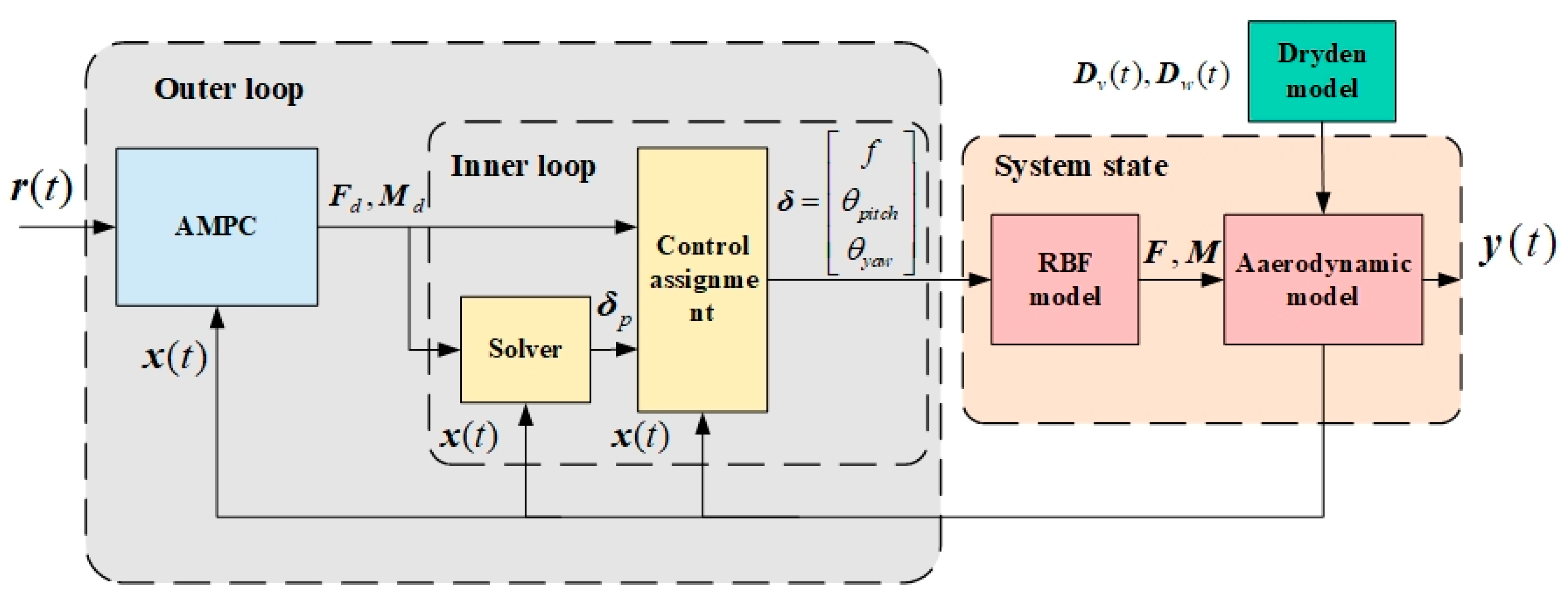
In the cascaded trajectory tracking control system structure, shown in Figure 5, the outer loop control law realizes the calculation of the trajectory command to the desired control aerodynamic force and torque ($F_d,M_d$), while the inner loop control assignment realizes the aerodynamic force and torque to the control command (flapping frequency, pitch angle, and yaw angle). This strategy is explained in detail in the following subsections.

By defining the output of the trajectory tracking controller as a virtual control quantity $v$, the entire control system of the CWMAV can be expressed as:

$$\begin{array}{l}{\dot{x}}_{total}=y(x_{total},v)\\ v=m(\mathit{x},\delta )\end{array}$$

(43)

where ${\mathit{x}}_{total}$ is the full state variable of the system, $\mathit{x}$ represents the state variable that affects the aerodynamic force and torque, $\mathbf{\delta }$ is the control parameter of the actual actuator, and $y, m$ are the system function and the control assignment mapping function, respectively.

After obtaining the mapping relationship between the control command and aerodynamic data, the nonlinear control assignment problem of the CWMAV can be transformed into a constrained optimization problem:

$$\begin{array}{l}\underset{\mathbf{\delta }}{\min }\hspace{1em}f(\mathit{x},\delta )={\Vert W_{\mathit{v}}(g(\mathit{x},\delta )-v)\Vert }_2\\ \mathrm{s}.\mathrm{t}.\hspace{1em}\underset{¯}{\mathbf{\delta }}\le \mathbf{\delta }\le \overline{\mathbf{\delta }}\end{array}$$

(44)

where $f\left(x,\delta \right)$ is the objective function of the optimization problem, selecting $L2$ as the performance index to reduce overfitting. $W_{\mathit{v}}$ is the weight matrix of the virtual control variable $v$. $\underset{¯}{\mathbf{\delta }}$ and $\overline{\mathbf{\delta }}$ are the strict lower and upper limits of the system actuator, respectively.

Considering the output interval and the maximum rate of change with the system actuator, $\underset{¯}{\mathbf{\delta }}$ and $\overline{\mathbf{\delta }}$ are expressed as:

$$\underset{¯}{\mathbf{\delta }}=\min \left({\mathbf{\delta }}_{\mathit{L}},\delta -{\dot{\mathbf{\delta }}}_{\mathit{max}}\Delta t\right),$$

(45)

$$\overline{\mathbf{\delta }}=\mathit{max}\left({\mathbf{\delta }}_{\mathit{U}},\delta +{\dot{\mathbf{\delta }}}_{\max }\Delta t\right),$$

(46)

where ${\mathbf{\delta }}_{\mathit{U}}$ and ${\mathbf{\delta }}_{\mathit{L}}$ are the upper and lower limit vectors of the actuator output, ${\dot{\mathbf{\delta }}}_{\max }$ represents the maximum change rate of the actuators, and $\Delta t$ is the controller update rate.

To solve no solutions or multiple solution problems of Equation (44), a regularization term is introduced to obtain a hybrid optimization to control the smoothness of the objective function:

$$\begin{array}{l}\underset{\mathbf{\delta }}{\min }\hspace{1em}f(\mathit{x},\mathbf{\delta })={\Vert W_{\mathit{v}}(g(x,\mathbf{\delta })-v)\Vert }_2+\lambda {\Vert W_{\mathbf{\delta }}(\delta -{\delta }_p)\Vert }_2\\ \mathrm{s}.\mathrm{t}.\hspace{1em}\underset{¯}{\mathbf{\delta }}\le \mathbf{\delta }\le \overline{\mathbf{\delta }}\end{array}$$

(47)

where $\lambda$ is the penalty factor for error minimization and control minimization. The value of $\lambda$ has a great influence on the results of the model. $W_{\delta }$ represents the weight matrix output by the actuators and ${\delta }_p$ is the preference vector of the control output. The purpose of adding a regularization item is to punish overfitting and avoid overfitting, thereby improving the generalization ability of the model. In this way, the complexity and accuracy of the optimization model can be balanced, and better results can be obtained.

2.3.2. Experimental Measurement

The numerical aerodynamic model is generally not accurate enough, with a much larger error than experimental data. To obtain the mapping function $m$ in Equation (43), a force measurement experiment is conducted in a low-speed tunnel (Figure 6).

The experiments were conducted in a low-speed wind tunnel. This is a closed-circuit facility with a rectangular cross-section of 1.2 m wide, 1.2 m high, and 3 m long. The entrance section is equipped with a regular hexagonal honeycomb and a five-layer 24 mesh/inch damping net. The four corners of the wind tunnel are installed with eight baffles. The fan in the power section of the wind tunnel has a diameter of 0.8 m and is composed of eight blades. It is driven by a variable frequency speed motor, and the rated speed of the motor is 986 r/min. Before the test section, the tunnel has an entry section with screens and a contraction ratio of 5:1 to ensure that the angle of wind deflection is lower than 0.5 degrees and the turbulence level is lower than 0.5 %. The tunnel flow speed was monitored by a pitot tube installed in the tunnel, and the free-stream speed was controlled by a manual speed controller that drove the tunnel fan, providing an experimental flow speed from 0.1 m/s to 5 m/s, which was also measured by a Pitot tube. The mechanical data acquisition system included a six-dimensional mechanical sensor (Nano 17), a data acquisition card (National Instruments, NI), and PC terminal mechanical data acquisition software. The number of bits, number of channels, protocols, sample rate, and connection type of the data acquisition card are 16, 16 single-ended, multifunction I/O, 250 KS/s, and USB, respectively.

The test prototype is a developed clapping-wing micro air vehicle. The initial state parameters include:

• Initial position: ${[x(0),y(0),z(0)]}^T={[2,-4,0]}^T \mathrm{m}$;
• Initial velocity: ${[V_x(0),V_y(0),V_z(0)]}^T={[0,2,0]}^T \mathrm{m}/\mathrm{s}$;
• Initial Euler angle: ${[\varphi (0),\theta (0),\psi (0)]}^T={[0,{30}^{\circ },{90}^{\circ }]}^T$.

As mentioned before, the rolling moment could be technologically ignored. $-0.05\le F_x\le 0.2, -0.03\le F_y\le 0.03, -0.05\le F_z\le 0.35$ and $-20\le M_y\le 20, -15\le M_z\le 15$ are the force and moment constraints of the optimization.

2.3.3. Radial Basis Function Modeling

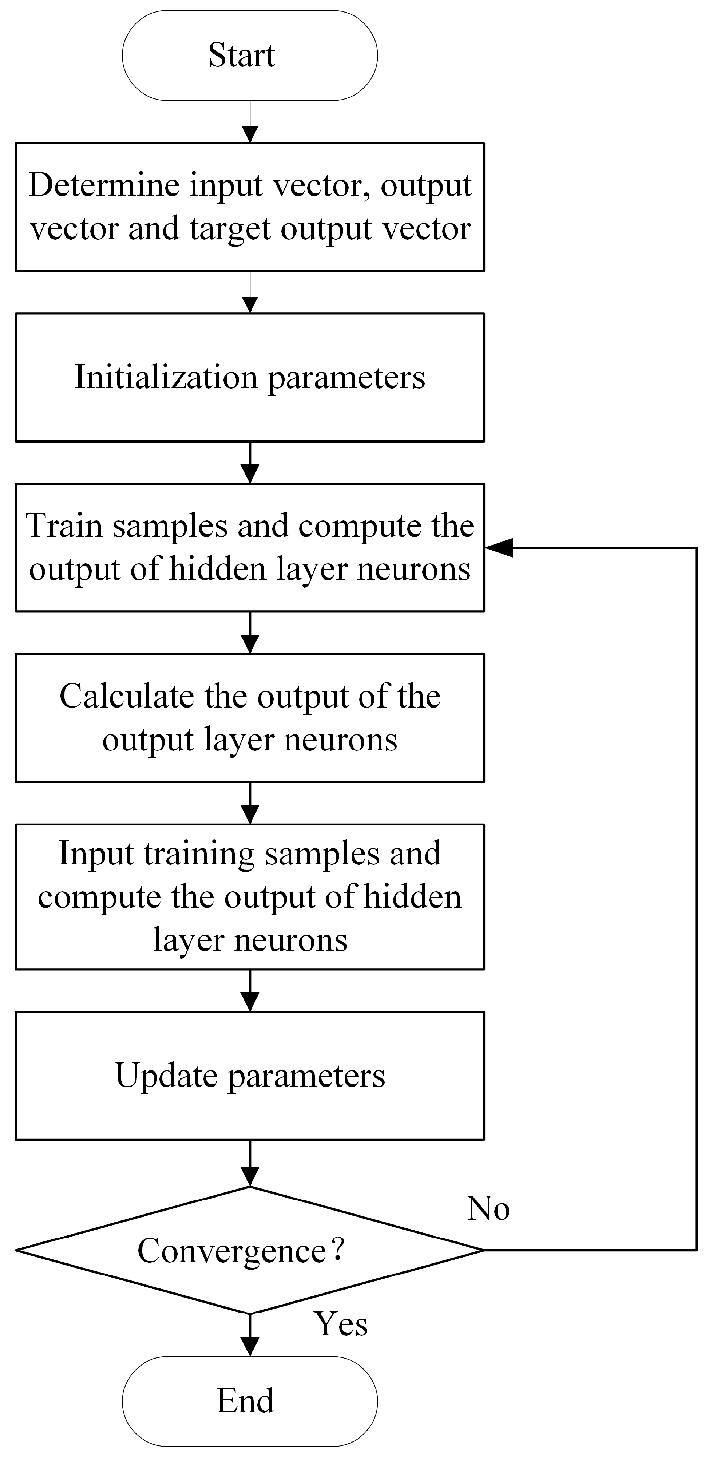
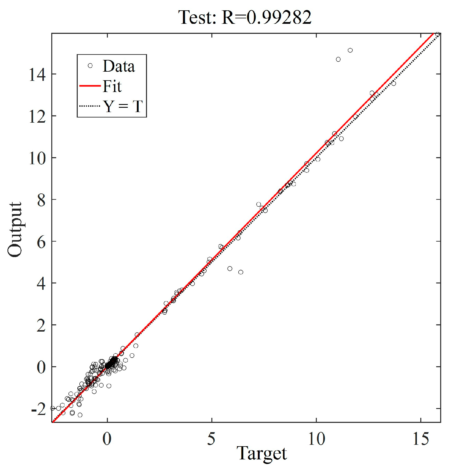
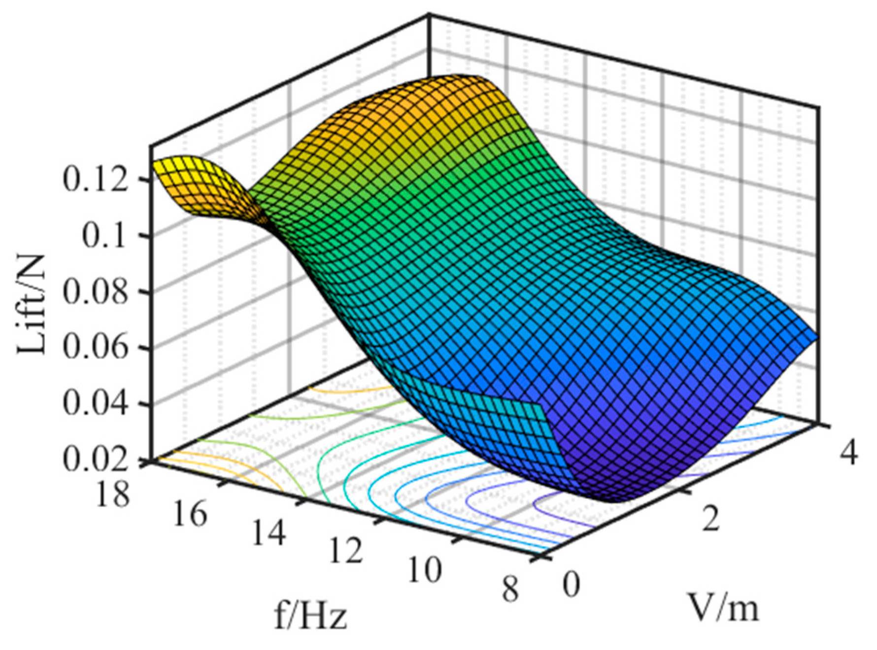
Due to the nonlinear characteristics and unsteady effects of the CWMAV, the radial basis function is adopted in this study to conduct the mapping function $m$ in Equation (43). The proposed aerodynamic modeling scheme is illustrated in Figure 7.

For the aerodynamic model of the CWMAV in this paper, the angle of attack and the incoming flow velocity are the state variables; the flapping frequency $f$, pitch angle ${\theta }_{pitch}$, and yaw angle ${\theta }_{yaw}$ are the design variables of the actuators. Therefore, the entire design variables are five-dimensional, and the outputs are six-dimensional.

3. Results and Discussion

3.1. Results of Radial Basis Function Modeling

The primary parameters of the RBF model adopted in this study are as follows: the number of nodes in each layer is 5E-6; the number of trainings is 1000 epochs; the learning rate is 0.1; the momentum factor is 0.01, and the network performance index is 1E-3. In order to prevent overfitting, this study divides the data into three parts: the proportions of training data, validation data, and test data are 70%, 15%, and 15 %, respectively. The obtained fitting results are shown in Figure 8 and Figure 9. It can be found that the mean square error is basically stable after 50 iterations, and the fitting correlation coefficient of the test set is above 0.99, leading to high fitting accuracy.

The response surface of the wind speed and flapping frequency are selected, as shown in Figure 10. It can be found that the nonlinearity of the model is relatively high; therefore, the linear programming method cannot solve the control assignment problem of the CWMAV. To figure out the optimization shown in Equation (44) based on the RBF aerodynamic model, a genetic algorithm (GA) is adopted to accelerate optimization solving.

3.2. Validation Studies

A validation simulation was conducted to verify the effectiveness of the trajectory tracking controller proposed in this study. The proposed observer-based RAMPC and the classical MPC method were compared under the conditions of free flight and internal uncertainties and external disturbances. The physical parameters of the CWMAV used in the validation study are listed in

Table 1. Physical parameters of the CWMAV.

Parameters	Physical Quantity	Magnitude	Unit
$\mathrm{m}$	Total mass	15.4	$\mathrm{g}$
$I_x$	X-axis moment of inertia	4.9 × 10−6	$\mathrm{kg}\cdot {\mathrm{m}}^2$
$I_y$	Y-axis moment of inertia	4.3 × 10−6	$\mathrm{kg}\cdot {\mathrm{m}}^2$
$I_z$	Z-axis moment of inertia	1.2 × 10−6	$\mathrm{kg}\cdot {\mathrm{m}}^2$
$I_{xz}$	Product of inertia relative to the X- and Z-axes	5.6 × 10−7	$\mathrm{kg}\cdot {\mathrm{m}}^2$

.

In the model predictive control, increasing the time domain range of the prediction output and the control input can generally increase the control accuracy and also significantly increase the computational scope of the model. After a series of tests, we found that there is no obvious increase when the solution range of the control input $N_u$ is more than six or the number of tests is more than ten. Therefore, $N_u=6, N=10$ are chosen as the values.

A radial function is used to solve the diagonal weight matrix $Q$, the control variable weight matrix $\mathit{R}=diag(0.1,0.15,0.2,0.25,0.3,0.35)$. The search step and the sampling time in Equation (32) are set to $\gamma =0.1$ and $T=0.02 \mathrm{s}$, respectively.

A trajectory (including forward flying, fixed altitude turning, and climbing) was used to verify the effectiveness of the proposed RAMPC, whose trajectory equation is shown in Equation (48). The entire trajectory covers the basic tracking tasks in the longitudinal and lateral planes, performing a quasi-actual flight condition.

$$\begin{array}{l}x(t)=2t\hspace{1em}\hspace{1em}\hspace{1em}\hspace{1em}\hspace{1em}\hspace{1em}\hspace{1em}0<t\le 30\\ y(t)=\{\begin{array}{l}0\hspace{1em}\hspace{1em}\hspace{1em}\hspace{1em}\hspace{1em}\hspace{1em}\hspace{1em}0<t\le 5\\ 5\sin (0.1\pi t-\pi )\hspace{1em}\hspace{1em}5<t\le 15\\ -10\hspace{1em}\hspace{1em}\hspace{1em}\hspace{1em}\hspace{1em}\hspace{1em}15<t\le 30\end{array}\\ z(t)=\{\begin{array}{l}0\hspace{1em}\hspace{1em}\hspace{1em}\hspace{1em}\hspace{1em}\hspace{1em}\hspace{1em}0<t\le 15\\ 5\sin (0.1\pi t)+5\hspace{1em}\hspace{1em}15<t\le 25\\ 10\hspace{1em}\hspace{1em}\hspace{1em}\hspace{1em}\hspace{1em}\hspace{1em}\hspace{1em}25<t\le 30\end{array}\end{array}$$

(48)

In the actual flight of the CWMAV, there are many time-dependent internal uncertainties and external disturbances. Therefore, a simulation experiment is conducted while considering these disturbances of the system to compare the performance of the closed-loop with the classical MPC controller.

Considering the change in the mass distribution of the CWMAV during flight, an additional 20% sinusoidal fluctuation to simulate internal uncertainties is added into the moment of inertia of the CWMAV, which is expressed as follows:

$$\{\begin{array}{l}{I}_x(t)={\overline{I}}_x+0.2{\overline{I}}_x\sin (2\pi ft)\\ I_y(t)={\overline{I}}_y+0.2{\overline{I}}_y\sin (2\pi ft)\\ I_z(t)={\overline{I}}_z+0.2{\overline{I}}_z\sin (2\pi ft)\end{array},$$

(49)

where $\overline{I}=[{\overline{I}}_x{\overline{I}}_y{\overline{I}}_z]$ is the extended diagonal positive definite matrix of $I$.

The Dryden wind turbulence model is applied (Figure 11) to simulate the external disturbances during the actual flight of the CWMAV.

3.3. 3D Tracking Effect of the RAMPC with Time-Dependent Disturbances

RAMPC with time-dependent disturbances was chosen as the most valuable validation case to show the tracking effect (Figure 12, Figure 13 and Figure 14).

From Figure 12 and Figure 13, it can be seen that the tracking trajectory of the RAMPC matches the desired output trajectory very well. The maximum error in the X-axis and Z-axis displacement tracking is not more than 0.2 m, and the minimum error is in the X-axis tracking, with approximately 0.05 m, resulting in a great tracking effect.

Figure 14 shows the curve of the attitude angle and actuator output of the CWMAV during trajectory tracking flight. Based on the mechanism of attitude control and attitude angle solving Equations (12)–(14), it can be found: (1) in the turning stage ($t=5\sim 15$), the yaw actuator and flapping frequency can work to provide roll and yaw torques; (2) in the climbing stage ($t=15\sim 25$), the pitch actuator and flapping frequency change to provide the pitch torque; (3) in the decelerating stage ($t=25\sim 30$), the amplitude of the flapping frequency decline is smaller than that of the accelerating stage, which is due to that a larger incoming flow speed could provide more resistance.

3.4. Comparisons of 3D Trajectory Tracking Simulation under Internal Uncertainties and External Disturbances

To further illustrate the tracking error,

Table 2. Root mean square error of controllers under external disturbances.

Type	Controller	RMSE (X-Axis)	RMSE (Y-Axis)	RMSE (Z-Axis)
Constant disturbances	RAMPC	0.0045	0.0552	0.0183
	MPC	0.0153	0.0778	0.0440
Improvement		70.6%	29.0%	58.4%
Time-dependent disturbances	RAMPC	0.0063	0.0628	0.0443
	MPC	0.0187	0.1108	0.0661
Improvement		66.3%	43.3%	32.9%

shows the tracking root mean square error of the MPC and RAMPC controllers under two types of external disturbances. It can be seen that the RAMPC has a smaller tracking error, with a decline of about $30\%\sim 70\%$.

These simulation results prove that the proposed RAMPC controller can effectively implement the trajectory tracking control of the CWMAV and that the mode has some ability to adapt to internal uncertainties and external disturbances. The performance of the RAMPC is much better than that of the classical MPC.

4. Conclusions

This study proposed a radial basis function model-based adaptive model predictive control (RAMPC) trajectory tracking control method for the problem of trajectory tracking of clapping-wing micro air vehicles (CWMAVs) in the presence of internal uncertainties and external disturbances. First, a calculation of the desired attitude is shown based on the desired trajectory equation and the current state, and two observers are introduced to estimate the model uncertainty and external disturbances simultaneously. Second, the radial basis function model-based control assignment model is designed from experimental measurements and incorporated into the adaptive predictive control model to obtain a closed-loop trajectory tracking control model. Validation studies demonstrate that the proposed RAMPC performs well in trajectory tracking under internal uncertainty and external disturbances. The RAMPC can provide a $30\%\sim 70\%$ tracking error decline to obtain better control effects.

The next step in the future is to explore multi-sensor information fusion techniques. Model-based control approaches increase the accuracy requirement for flight state feedback. Developed multi-sensor information fusion technologies will ensure the measurement accuracy of onboard sensors and support autonomous flight.