Static Aeroelastic Optimization of High-Aspect-Ratio Composite Aircraft Wings via Surrogate Modeling

Abstract

The race towards cleaner and more efficient commercial aviation demands novel designs featuring improved aerodynamic and structural characteristics, the main pillars that drive aircraft efficiency. Among the many proposed and introduced, the increase in the aspect ratio of the wings enables greater fuel efficiency by reducing induced drag. Nevertheless, such structures are characterised by elevated flexibility, aggravating static and dynamic aeroelastic phenomena. Consequently, the preliminary and conceptual design and optimization stages using high-fidelity numerical tools is rendered extremely intricate and prohibitive in terms of computational cost. Low-fidelity tools, contrastingly, enable computational-burden alleviation. In our approach, a computational framework for the low-fidelity steady-state static aeroelastic optimization of a composite high-aspect-ratio commercial aircraft wing via surrogate modelling is proposed. The methodology starts with the development of the 3D panel method as well of the elements of the surrogate model. The design variables, objective function and constraints which formulate the optimization problem are then provided. Moreover, comparison against rigid aerodynamics indicate the significant load-alleviation capabilities of the present case study. The effect of structural nonlinearities is also explored. The optimization framework is executed and optimal laminates for the structural members are obtained. The optimal structure was deemed critical in panel buckling.

1. Introduction

Over the past decades, the airline industry and, particularly, commercial aviation has been vastly expanding, rendering flight an indispensable means of transportation around the globe in our modern societies. This trend is expected to carry on in the foreseeable future, as indicated by the latest predictions made by the two main shareholders of commercial aviation, namely, Airbus and Boeing. In particular, in its commercial market outlook [1], Airbus foresees an 4.3% annual air-traffic growth by means of the Revenue Passenger Kilometer (RPK) index, over the next 20 years. Similarly, Boeing also envisages, via the “Commercial Market Outlook, 2021–2040” [2], a 4% worldwide RPK growth rate, calculated from years 2019 to 2040. Despite the facilitation of transportation and the associated stimulation of the global economies, the current and forthcoming air-traffic proliferation has severe ramifications and impacts on the environment. The emission of greenhouse gases, mainly in terms of carbon dioxides (CO₂) and nitrogen oxides (NOx), and their corresponding concentrations in the atmosphere is expected to be exacerbated, possibly leading to the constitution and dissemination of severe public-health-related threats. To that end, and as a remedy, the European Commission envisages, through the definition of ACARE FlightPath 2050 [3] among others, a reduction by 75% in CO₂ emissions and by 90% in NOx, per passenger km, for future commercial transport aircrafts. A key enabler for this effort, allowing for around 20% to 25% reduction in the aforementioned quantities, is the introduction of novel, more efficient airframe designs with improved aerodynamic and structural characteristics. From an aerodynamics point of view, the aerodynamic efficiency of an aircraft is closely related to the aspect ratio of the wings, with higher aspect ratios reducing the induced drag force and increasing the lift-to-drag ratio, which, in turn, enhances fuel efficiency. Therefore, an increasing trend in the aspect ratio of commercial aircraft wings over the past decades is observed [4], with current efforts endeavoring to further push design envelopes.

The nature and elevated complexity of the aforementioned aircraft design novelties, introduced by the aerodynamics and structures disciplines, pose serious challenges to the scientific community, rendering the design of air vehicles a matter of increasingly extensive research studies. One of the most prominent and challenging phenomenon emanates from the increase in aspect ratio and the accompanied elevated flexibility of the wing which, on one hand, induces a closer coupling between the structure and the surrounding fluid, aggravating static and dynamic aeroelastic phenomena. Additionally, the ever-increasing use of composite materials [5] complicates the design optimization procedure by vastly increasing the design space via the introduction of new variables such as ply thickness and ply orientation. As a result, the development and embodiment, in a typical aircraft design process, of novel design methodologies and computational tools capable of capturing and predicting the whole spectrum of phenomena inherent to this new generation of structures, as well as producing optimum configurations, is of paramount importance. Furthermore, the aforementioned set of tools should ideally include certain attractive characteristics such as low computational time along with high levels of accuracy, in order to efficiently drive the design process towards optimal configurations. Since this often constitutes a utopian scheme, a vast variety of multi-fidelity tools, each achieving different levels of accuracy, efficiency and ability to capture the physical phenomena present, has emerged and is typically designated at each design stage. Commonly, a three-stage design process spans the development of an aircraft, namely, the conceptual, the preliminary and the detailed [6]. Over the course of time, multi-fidelity computational tools, with application in a plethora of analysis disciplines, have been designated to a corresponding design stage mainly based on their attributes, as stated earlier. In the early design stages, one enjoys immense design freedom, albeit counterbalanced by little-to-no design knowledge. Low-fidelity computational tools along with statistical models and empirical knowledge are, therefore, preferred due to their fast modeling and turnaround times, even though they typically suffer from limiting accuracy and ability to capture higher order phenomena and nonlinearities. As the design process and knowledge on the current candidate configuration matures, higher fidelity tools which can replicate and resolve the complex phenomena that might be present with greater accuracy come into play in exchange for increased and occasionally prohibitive computational cost. In these stages, the design freedom is highly restricted, and any design alteration could induce severe cost penalties. As a result, and since also historically the majority of the design effort is put into the conceptual and preliminary design phases [7] and any design change between phases could be costly, the accuracy of low- and medium-fidelity models is usually sought to be to be enhanced and further exploited. In this manner, design-space exploration is reinforced by alleviating the computational burden, steering the design process towards optimality and, in general, towards a better and more reliable decision-making process by providing a wider understanding of a candidate design. Finally, yet importantly, and throughout the design stages, all relevant tools are coupled with optimization algorithms in order to gain further knowledge regarding the design space, as well as to obtain the corresponding optimum solution with respect to the objective functions set.

In terms of low-fidelity models, typically planar panel methods such as the vortex lattice method (VLM) and the doublet lattice method (DLM) are introduced for aerodynamics and are coupled with reduced-order or finite element method (FEM) models of the structure [8,9,10,11]. The inclusion of aeroelastic effects via fluid-structure interaction (FSI) techniques is also conducted at this level of fidelity [12,13], but it typically occurs in high-fidelity solvers, employing Euler or Reynolds-averaged Navier–Stokes (RANS) [14,15,16]. Serious challenges arise, nevertheless, from the realization of such algorithms, the main culprits being the possible deterioration of the aerodynamic mesh quality upon structural deformation, an effect which is exacerbated for high-aspect-ratio wings, as well as the elevated computational time. For the latter, inclusion in optimization algorithms constitutes an active research area, due to the complex nature of the problem [17,18,19].

Comparison among the low and high-fidelity models was conducted in terms of aerodynamic loads, flutter and divergence limit speed in [15,20]. Despite the inability to accurately capture instabilities that typically occur in the transonic regime, e.g., transonic dip [21], the steady-state static aeroelastic response of a contemporary airliner wing as predicted by 3D panel methods was in excellent agreement with high-fidelity Euler and RANS solutions, even at the transonic regime [22]. In [23], significant changes in the required angle of attack to attain the targeted lift load for a modified CRM wing were obtained by the inclusion of high-fidelity aerodynamics. Nevertheless, for rigid aerodynamics, no significant mass changes were noticed following a single-pass structural optimization stage, implying the correct representation of the lift load.

Even for low-fidelity models, the inclusion of static aeroelastic effects in optimization frameworks, able to reflect on the influence of the design parameters and changes in the final design, often render the numerical optimization tedious in terms of computational cost. The black-box nature of the objective and constraint functions also complicates the evaluation of gradients and, as a result, the use of gradient-based optimization algorithms. Furthermore, gradient-free algorithms may suffer from slow convergence and lack of a true optimum solution, as mentioned in the previous section [24]. As a result, the optimum is sought via relatively fast mathematical techniques to approximate the underlying objective function, aiming at achieving a good trade off between accuracy and computational speed as well as between the global and local exploration of the design space. To that end, surrogate modeling techniques [25,26] have started to draw the attention of the scientific and engineering communities. Such techniques can be used solely for approximations of the underlying functions as well as being cast into surrogate-based optimization (SBO) frameworks, which adopt updated techniques in order to enhance the accuracy of the model and guide the optimization towards the global optimum [27,28,29,30]. Neural networks, radial basis functions (RBF), Kriging and support vector regression (SVE) constitute typical approaches toward surrogate models.

Despite the omnipresence of low-fidelity optimization frameworks, studies of optimization frameworks including static aeroelastic effects for composite-material high-aspect-ratio wings are rarely documented in the literature. This knowledge gap is aggravated when examining embodiment of such tools in SBO frameworks. Aiming to address this issue, this research study provides an efficient structural SBO framework of a high-aspect-ratio composite-materials aircraft wing subject to local panel buckling and strength and flutter constraints. The present study focuses on the development of an in-house SBO optimization technique, encapsulating a low-fidelity steady-state FSI scheme based on a 3D panel method for the sizing of a reference wing. This framework allows, on the one hand, for reductions in terms of computational costs during the optimization process in the preliminary design stages, while, in parallel, accounting for the effect of the elasticity on the structural response, which is of paramount importance to this generation of structures. The structure is parametrized in terms of the thickness of the structural members involved, with the minimization of the structural mass of the wing being set as the objective function. Design-strength, panel-buckling and flutter-instability constraints formulate the optimization problem. Overall, the applicability of the developed SBO framework to novel composite-materials aircraft wings constitutes a step towards more sophisticated and holistic numerical tools for the conceptual and preliminary design stages.

2. Materials and Methods

In this section, the cornerstones of this research are presented individually. Starting from the in-house developed 3D panel method for aerodynamic analyses, we then proceed to the particulars of the DLM aerodynamics model used for flutter calculations, the surrogate modeling techniques implemented herein and, finally, manifest the overall SBO framework.

2.1. 3D Panel Method

The main underlying assumptions of the in-house developed 3D panel method is that the flow is inviscid, irrotational and incompressible. For such flows, there exists a potential function $\Phi$ which satisfies the Laplacian equation:

$${\nabla }^2\Phi =0$$

(1)

For the solution of the Laplacian equation, elementary flow solutions in terms of sources and doublets are distributed on the surface of the wing and the wake. Along with the introduction of Green’s identity, Equation (1) is recast in the following form:

$$\Phi =\frac{1}{4\pi }{\int }_{wing+wake}{\mu }_p\mathit{n}·\nabla \left(\frac{1}{r}\right)dS-\frac{1}{4\pi }{\int }_{wing}\sigma \left(\frac{1}{r}\right)dS+{\Phi }_{\infty }$$

(2)

where $\mathit{n}$ is the surface normal vector, r the distance vector and ${\Phi }_{\infty }$ the free-stream potential function. For a discretized surface consisting of N wing and $N_w$ wake panels, integration of Equation (2) along with the application of the Kutta condition to the trailing edge panels can be further simplified into [31]:

$$\sum _{k=1}^{N_{panels}}{A}_{1k}{\mu }_k+\sum _{k=1}^{N_{panels}}{B}_{1k}{\sigma }_k=0$$

(3)

where $A_{1k}$ and $B_{1k}$ are the doublet and source influence coefficient for the kth panel, respectively. It should be also pointed out that a Dirichlet boundary condition is also specified at each of the panels at the collocation point. Setting the source terms on the right-hand side of Equation (3) equal to ${\sigma }_k={\mathit{n}}_k·U_{\infty }$, a set of linear equations that can be solved for the unknown doublet distribution is obtained. Making use of spatial interpolation schemes, one can calculate the induced velocities and, via application of the Bernoulli equation, the pressure coefficients on each panel. To account for possible compressibility effects in the flow, the Prandtl–Glauert correction factor was also implemented. Additionally, the wake of the wing was considered to be fixed and extending in the chordwise direction, with wake shape calculations being beyond the scope of this study. The results of the 3D panel method developed within the framework of this study were also verified and validated against CFD analyses and experimental results for the ONERA M6 wing case study [32], and are presented in Appendix A.

The developed 3D panel method enables the steady-state static aeroelastic computation of aircraft wings in a staggered FSI scheme. In particular, the following computational procedure is applied, with the relevant flowchart being presented in Figure 1:

• Given the initial geometry, perform an aerodynamic analysis and obtain the pressures in the aerodynamic panels.
• Since the aerodynamic and structural meshes coincide, transfer pressures to the structural elements.
• Perform a static linear analysis and obtain displacements.
• Update the current geometry.
• Check convergence in loads and displacements for the current iteration.
• If convergence is not achieved, perform an aerodynamic analysis to obtain new pressure field and repeat the analysis cycle until convergence criteria are met.

Due to large displacements involved in the analysis of high-aspect-ratio wing, often displacements under-relaxation factors (URF) are introduced to the solution procedure described earlier [33,34,35], aiming at achieving faster convergence algorithmic characteristics as well as avoiding possible divergence issues. Specifically, given the displacements vector solution of the structural subsystem at iteration n, ${\tilde{u}}_s^{(n+1)}$, and the current value of the relaxation factor, ${\theta }^{\left(n\right)}$, the under-relaxed displacements that will be used at the next iteration to update the motion of the fluid mesh are given by the following, Equation (4):

$$u_s^{(n+1)}=u_s^{\left(n\right)}+{\theta }^{\left(n\right)}\Delta {\tilde{u}}_s^{\left(n\right)}$$

(4)

where $\Delta {\tilde{u}}_s^{\left(n\right)}$, the increment in displacements, is defined as:

$$\Delta {\tilde{u}}_s^{\left(n\right)}={\tilde{u}}_s^{(n+1)}-u_s^{\left(n\right)}$$

(5)

The displacements $u_s^{(n+1)}$ are then used to deform the aerodynamic mesh and provide a new set of aerodynamic loads. The convergence characteristics of the proposed FSI algorithm are investigated in Section 3.2 given the applied aerodynamic loading as well as the developed reference wing FEM model.

2.2. DLM Aerodynamics Model

For the calculation of possible flutter instabilities that might be present, the p-k method implemented in NASTRAN SOL 145 is used. In particular, NASTRAN utilizes flat-plate DLM unsteady aerodynamics [36,37] for the calculation of the aerodynamic influence coefficient (AIC) matrices. Aerodynamic surfaces are typically divided into small trapezoidal panels and a constant pressure distribution is assumed. The DLM is capable of modeling unsteady flows in the frequency domain and is based on the linearized small disturbance potential flow equation, hence neglecting large perturbations and shockwaves:

$$(1-M_{\infty }^2){\Phi }_{xx}+{\Phi }_{yy}+{\Phi }_{zz}-2(\frac{M_{\infty }^2}{U_{\infty }}){\Phi }_{xt}-(\frac{M_{\infty }^2}{U_{\infty }}){\Phi }_{tt}=0$$

(6)

where $M_{\infty }$ and $U_{\infty }$ the free-stream Mach number and velocity, respectively, and ${\Phi }_{xx}$, ${\Phi }_{yy}$, ${\Phi }_{zz}$, ${\Phi }_{xt}$, and ${\Phi }_{tt}$ are second derivatives of the potential function. Assuming small amplitude and harmonic motion, solution to Equation (6) is given by the so-called acceleration potential and by introduction of doublets across the discretized planar lifting surface. The doublet line of constant value is placed at the 1/4th of the chord of each panel, while the normal wash collocation point, where the impermeability boundary condition is applied, is placed at the 3/4th of the chord. The resulting pressure coefficient for a panel i, denoted as ${\overline{p}}_i$, is expressed in terms of a complex matrix $A_{ij}$ [36], including the contribution of the generated downwash from panel j to panel i, and the downwash value ${\overline{w}}_i$ at the current panel of interest:

$${\overline{p}}_i=\sum _{j=1}^{N_{panels}}{A}_{ij}{\overline{w}}_j=\left[{AIC(M_{\infty },k)}_{ij}\right]w_j$$

(7)

Complex valued matrix $A_{ij}$ is now subject to evaluation given the discretized aerodynamic surface, the operating Mach number as well as the reduced frequencies k. The developed DLM aerodynamics model is presented in the following Figure 2.

The aerodynamic loads are transferred to the structural FEM model via infinite plate splines [38]. The structural nodes chosen for interpolation purposes, illustrated in Figure 3, are located at the front and rear spar as well as rib webs, allowing for better load distribution and avoiding local loading effects. For the purpose of the analysis, a set of 20 reduced frequencies were also used to calculate and interpolate, in user-defined velocities, the reduced-frequency-dependent aerodynamic loads. Possible flutter instabilities were then investigated for the first ten structural modes via the velocity-damping (V-g) and velocity-frequency (V-f) plots. In particular, the trends of each mode were monitored regarding the damping values, with positive damping indicating a possible flutter instability. The corresponding flutter velocity was then calculated via linear interpolation between the previous and subsequent velocities and damping values.

2.3. Surrogate Modeling

The basic steps involved in a typical SBO technique are the following [39]:

• Sampling of the design space and subsequent evaluation of the objective function and constraints.
• Selection and construction of the surrogate model.
• Search and update the surrogate model via update (infill) criteria.
• Enhance the model with the newly added point and reiterate.

The sampling stage is one of the most important stages of an SBO algorithm, since the construction of the surrogate model is based on the selection of the initial points on the design space. Therefore, the most important and influential points need to be selected in order to be as representative of the design space as possible and, as a result, maximize the information passed towards the surrogate model. Since large sets of design variables are often involved, full grid searches are prohibitive in terms of computational cost and more efficient methods, such as the latin hypercube sampling (LHS) [40] are often sought. LHS is a robust statistical method aiming at the generation of samples of parameter values from a multidimensional distribution. LHS involves, inherently, an optimization problem and, hence, some randomness in the results, since it seeks to maximize the distance between the samples under the constraint that the projection on each axis follows a predefined probability distribution.

Moving on to the surrogate model construction, a general model structure, $\widehat{f}(\mathrm{x},w)$, is a function of its parameters w as well as of the variables vector $\mathrm{x}$. A driving factor towards model selection is the ability of the model to capture the attributes of the desired function as well as to pertain flexibility characteristics, thus avoiding being too stiff, becoming unstable and overfitting the data. Turning our attention towards the Kriging model, which is a well-established surrogate model in the engineering field, approximations are in the form of a linear combination of basis functions (also called kernels), expressed as a function of the Euclidean distance between the design points. For noise-free data, the model obtains the following form:

$$\widehat{f}\left(\mathrm{x}\right)=\sum _{n=1}^{N_c}{\mathbf{w}}_n\psi \left(\right||\mathrm{x}-{\mathrm{x}}_c^{\left(n\right)}\left|\right|)$$

(8)

where $N_c$ denotes the number of basis functions included in the approximation, ${\mathrm{x}}_c^{\left(n\right)}$ the n-th center point of the $N_c$ basis functions and $\psi (||\mathrm{x}-{\mathrm{x}}_c^{\left(n\right)}||)$ the kernel function evaluated using the distance between the prediction point $\mathrm{x}$ and the corresponding centre point. The Kriging model assumes that the data stem from a stochastic process and that the model generated is the one most likely to have produced the training data results and has the following basis:

$$\psi =exp(-\sum _{n=1}^{N_c}{\theta }_n\left(\right||\mathrm{x}-{\mathrm{x}}_c{\left|\right|)}^{p_n}$$

(9)

with ${\theta }_n$ and $p_n$ constituting the parameters of the model. The Kriging model is then built via the following steps:

• Formulate the correlation matrix based on the training data points

  $$[\mathbf{\Psi }]=corr(Y(x^{(i)}),Y(x^{(l)}))=exp(-\sum _{n=1}^{N_c}{\theta }_n\left(\right||{\mathrm{x}}_n^{\left(i\right)}-{\mathrm{x}}_n^{\left(l\right)}{\left|\right|)}^{p_n}$$

  (10)
• Maximize the maximum likelihood estimator (MLE) as presented in Equation (11), expressed via the concentrated ln-likelihood function and obtain $\theta$. In our case, $\mathbf{p}$ was set to 2.

  $$ln\left(MLE\right)=-\frac{n}{2}ln\left({\widehat{\sigma }}^2\right)-\frac{1}{2}ln\left([\mathbf{\Psi }]\right)$$

  (11)

  where $\widehat{\sigma }$ is MLE estimate of the standard deviation
• The Kriging predictor at a new point of the design space is then calculated as follows:

  $$\widehat{y}\left(\mathrm{x}\right)=\widehat{\mu }+{\mathbf{\psi }}^T{[\mathbf{\Psi }]}^{-1}(\mathbf{y}-1\widehat{\mu })$$

  (12)

  where $\widehat{\mu }$ is MLE estimate of the mean and $\mathbf{\psi }$ a correlation vector between the observed data and the prediction point.

Within a typical SBO approach, model updating can be either conducted via searching the surrogate model for the current optimum and reconstructing the model with this value for a number of predefined iterations or, and as stated earlier for the Kriging model, utilizing the error estimation metric available for the objective function. In particular, the mean squared error (MSE) estimation for a Gaussian-based process is given by the following equation.

$$\widehat{s}{\left(\mathrm{x}\right)}^2={\widehat{\sigma }}^2(1-{\mathbf{\psi }}^T{[\mathbf{\Psi }]}^{-1}\mathbf{\psi }+\frac{1-{\mathbf{1}}^T{[\mathbf{\Psi }]}^{\mathbf{-}1}\mathbf{\psi }}{{\mathbf{1}}^T{[\mathbf{\Psi }]}^{-1}\mathbf{1}})$$

(13)

Since not only the uncertainty but also the promising regions of the current iterate of the surrogate are suitable for a model, updatingimproves the best observed value. A widely used estimator is the expected improvement function, reflecting the amount of improvement expected over the current minimum value. The metric is formulated by the following, Equation (14):

$$E\left[I\left(\mathrm{x}\right)\right]=(y_{min}-\widehat{y}\left(\mathrm{x}\right))\Phi (\frac{y_{min}-\widehat{y}\left(\mathrm{x}\right)}{\widehat{s}\left(\mathrm{x}\right)})+\widehat{s}\left(\mathrm{x}\right)\varphi (\frac{y_{min}-\widehat{y}\left(\mathrm{x}\right)}{\widehat{s}\left(\mathrm{x}\right)})$$

(14)

where $\Phi$ and $\varphi$ are the cumulative distribution and probability density function, respectively. As an additional step towards more realistic SBO frameworks, constraints should be added to the surrogate model. Depending on the cost of the constraint function evaluation, the constraints can be either evaluated directly or utilize similar concepts to the ones presented earlier for the objective function, thus constructing a surrogate model for each constraint. When constraints are cheap to evaluate, the concepts of constraint optimization introduced earlier are used along with the objective function surrogate model to guide the SBO framework towards not only promising but also feasible regions of the design space. Should surrogate models be preferred for a constraint as well, the expected improvement function in Equation (14) is modified to the constrained expected improvement via introduction of the probability of feasibility function:

$$P\left[F\left(\mathrm{x}\right)\right]=\frac{1}{\widehat{s}\left(\mathrm{x}\right)\sqrt{2\pi }}{\int }_0^{\infty }exp(\frac{-{(F-\widehat{g}\left(\mathrm{x}\right))}^2}{2\widehat{s}{\left(\mathrm{x}\right)}^2})dG$$

(15)

where F the measure of feasibility of a constraint g and $\widehat{s}$ the variance of the constraint Kriging model. The probability of an improvement over the current function minimum, while being feasible, is given by multiplication of Equations (14) and (15):

$$E\left[I\right(\mathrm{x})\cap F(\mathrm{x}\left)\right]=E\left[I\right(\mathrm{x}\left)\right]·P\left[F\right(\mathrm{x}\left)\right]$$

(16)

For the aforementioned update strategy, the next infill point is then found as the solution of a sub-optimization problem:

$${\mathrm{x}}_{infill}=argmax(E\left[I\left(\mathrm{x}\right)\right]·P\left[F\left(\mathrm{x}\right)\right])$$

(17)

2.4. SBO Framework

2.4.1. Objective Function and Design Constraints

Within the framework of our study, the minimization of the mass of the wing constitutes the objective function subject to design constraints in terms of static strength, panel buckling and aeroelastic instabilities in terms of flutter velocity. Since no explicit static stiffness requirements do exist in the literature for this generation of aircraft wings, such constraints are not imposed. As far as the static strength is concerned, a first-ply failure (FPF) via the Tsai–Wu criterion [41,42] is used for the strength prediction in terms of the failure index (FI) of the composite skins, spar and rib webs. For the rest of the parts, a direct comparison between the maximum stress and the corresponding material-strength value was performed in order to obtain the FI for the wing component under consideration. Regarding the buckling constraints, a global–local FEM modeling technique was implemented for the panels of the upper and lower skins within the framework of this study. A panel is considered as the intersection between the front and rear spar as well as two adjacent ribs, as indicated in Figure 4. As far as the global–local modeling technique is concerned, the resulting nodal displacements at each of the four edges of each panel of the global FEM act as input boundary conditions to the local-level FEM analysis. Since dissimilar meshes were considered, interpolation schemes were employed at each edge of each panel in order to calculate the local displacement field at intermediate positions. Furthermore, and at this level, blade stiffeners were considered and modeled explicitly via CQUAD4 elements. Buckling analyses were executed for each of the panels present in the wing via the SOL 105 solver implemented in NASTRAN, with the first buckling eigenvalue (BE), namely, the critical buckling load, expressed as a percentage of the originally applied load, being the quantity of interest. The minimum eigenvalue should then be greater than unity in order to avoid any buckling failure.

To avoid local-maximum-stress-driven designs, while simultaneously keeping the number of constraints for the optimization problem to a minimum, the constraint aggregation technique of Kreisselmeier–Steinhauser (KS) was employed [43,44] for the static strength as well as buckling constraints. For a problem consisting of $N_c$ quantities of interest, g, having a maximum value of $g_{max}$, the KS functions are of the following form:

$$KS\left(g_j\right)=g_{max}+\frac{1}{\rho }ln[\sum _j^{N_c}exp(\rho (g_j-g_{max}))]$$

(18)

and are formed separately for the calculated FI of each of the components involved in the static strength as well as for each upper-panel-buckling critical-load evaluation procedure. The aggregation parameter $\rho$ was set to 100 for all KS functions. This value has been reported in structural optimization studies of the CRM wing [45,46] and is shown to provide accuracy of the optimal solution.

Completing the set of constraints, the dynamic aeroelastic instability by means of flutter velocity of the candidate design solutions was also investigated, as described in Section 2.2. The flutter velocity was then constrained to be less than 1.2 times the design dive speed, $V_D$, which was set to 221.7 m/s equivalent airspeed (EAS), as in [47]. For the SBO framework, and in case no flutter point was calculated, the flutter velocity was set to a value outside of the velocity range of the analysis. The objective function as well as the constraints of the SBO framework are summarized in

Table 1. Optimization problem setup.

Objective Function	Minimize Structural Mass
Under the Constraints
Constraint Type	Limit Value
KS(FI), upper skin	≤1
KS(FI), lower skin	≤1
KS(FI), spar caps	≤1
KS(FI), spar webs	≤1
KS(FI), rib webs	≤1
KS(FI), rib caps	≤1
KS(FI), stringers	≤1
KS (BE), upper skin	≥1
KS (BE), lower skin	≥1
Flutter speed	≥1.2 ·$V_D$

.

2.4.2. Design Variables

The thickness of the skins, spar and rib webs and caps as well as of the stringers constitute the variables of the optimization problem. To allow for a wider design space, the wing was divided in 8 spanwise optimization zones, as illustrated in Figure 5. To reduce the number of variables associated, a spanwise linear thickness decrease was assumed for all of the components of the wing. To further reduce the dimensionality of the optimization problem, while in parallel achieving conformity to the SBO guidelines as presented in [26], minimum ply percentages and type of materials at each component were predefined as in [18] and are presented in

Table 2. Laminate percentages and materials applied at the SBO.

Component	Ply Percentages $<0^{\circ },{90}^{\circ },{45}^{\circ }/$−${45}^{\circ }>$, %	Material
Skins, Caps and Stringers	$<60,15,25>$	Hexcel 8552/IM7 UD
Webs	$<25,25,50>$	PW/AS4 Fabric

.

For the definition of the stacking sequence, a library of predefined symmetric and balanced laminates for various percentages of 0${}^{\circ }$, 90${}^{\circ }$ and 45${}^{\circ }$/−45${}^{\circ }$ plies was generated. In particular, the following laminates were considered:

$$ComponentLayup=[{\left({{45}_{\left(n_1\right)}/0_{\left(n_2\right)}/-{45}_{\left(n_1\right)}/{45}_{\left(n_3\right)})}_{ns}\right]}_s^{\left(z\right)}$$

(19)

where $\left(z\right)$ is the optimization zone; and $n_1$, $n_2$, $n_3$ integers were allowed to vary between 1 and 10. The number of symmetric blocks, $ns$, was also set as a variable. The former parametrization enables the generation of balanced and symmetric laminates, hence conforming to composite-materials design guidelines [48]. Furthermore, the various thickness variables (of continuous nature) provided by the SBO framework can be associated with a specific laminate. Since exact matching of the target and actual thickness values is not attainable, the closest to greater values of the target thickness and ply percentages is preferred. A summary of the parameters of the SBO framework is provided in the following

Table 3. SBO framework parameters.

Parameter	Value
Nr of variables	27
Initial sampling size	20
Infill Iterations	80

.

Overall, the proposed SBO framework, illustrated in Figure 6, consists of two main stages, namely, the sampling and model updating stages. The process starts with the definition of the sampling size and the subsequent generation of samples based on the LHS, as described earlier. The objective function and constraints are then calculated via execution of the FSI analysis framework (Figure 1). Following the training stage, the main SBO framework is executed. The hyperparameters of the Kriging model of the objective function and constraints are initially obtained. The constrained expected improvement function (Equation (15)) is then minimized via a sub-optimization routine and a new point in the design space is obtained. The FSI analysis is then re-executed on the new point and the model is updated. The process is executed for a predefined number of infill points.

3. Results

3.1. Main Case Study

Within the context of this work, the undeflected CRM, namely, uCRM-13.5, was chosen as the reference wing model. Constituting a modified, high-aspect-ratio derivative of the original CRM wing [49], the uCRM-13.5 model [50] serves as a benchmark configuration for CFD and the aerostructural optimization studies of realistic, contemporary as well as future aircraft configurations. The relevant geometric data are summarized in the following,

Table 4. uCRM-13.5 geometric characteristics.

Entity	Value
Wingspan	72 m
Root chord	11.07 m
Tip chord	2.06 m
Reference area	383.78 m2
Taper ratio	0.25
Aspect ratio	13.5
Quarter chord sweep angle	35${}^{\circ }$
Yehudi chord	7.56 m
MAC	5.77 m

:

Regarding the internal configuration, two spars located at 10% and 60% of the local chord are present along with 54 evenly distributed ribs and upper and lower skin stiffeners. Spar and rib caps were also included within the framework of this study, in contrast to the internal configuration presented in [50]. These primary load-carrying components are commonly found in a commercial airliner’s wingbox; hence, their effect and influence in the overall stiffness and strength of the structure were deemed necessary to be investigated, as demonstrated in later sections. An exploded view of the internal structure is illustrated in the following, Figure 7. For the sake of clarity, the spar and rib caps as well as the stiffeners are depicted via spanwise straight lines.

In our case and based on the external geometry and internal configuration of the reference wing, an FEM model was developed in NASTRAN. Specifically, the upper and lower skins along with the spar and rib webs were modeled via 4-noded quadrilateral shell elements, denoted as CQUAD4. On the other hand, the spar and rib caps as well as the skin stiffeners are assumed, as per common practise, to be modeled via beam elements (denoted as CBEAM) along with the relevant offset values. As a datum design point, a reference balanced and symmetric layup and, specifically, the [(45/0/−45/90)_2s]_s were considered for all the relevant wing parts. Furthermore, similarly to [17,18], the upper and lower skins were assumed to be manufactured of the Hexcel IM7/8552 UD [51] composite material, while the spars and ribs of the PW Fabric AS4/8552 [52], with the respective material properties, cured ply thickness, density as well as strength values, listed in

Table 5. Composite-materials properties.

Material	${\mathit{E}}_1$	${\mathit{E}}_2$	${\mathit{G}}_{12}$	${\mathit{G}}_{13}$	${\mathit{\nu }}_{12}$	${\mathit{X}}_{\mathit{T}}$	${\mathit{X}}_{\mathit{C}}$	${\mathit{Y}}_{\mathit{T}}$	${\mathit{Y}}_{\mathit{C}}$	S	$\mathit{\rho }$	Ply Thickness
	[GPa]	[GPa]	[GPa]	[GPa]		[MPa]	[MPa]	[MPa]	[MPa]	[MPa]	[kg/${\mathbf{m}}^3$]	[m]
Hexcel IM7/8552	158.51	8.96	4.68	4.68	0.315	2500	1531	640.5	285.7	53.5	1590	$1.8288\times {10}^{-4}$
PW AS4/8552	64.53	65.57	4.96	4.96	0.04	751.6	793.8	742	752	56	1570	$1.9281\times {10}^{-4}$

. Simple rectangular cross-sections were chosen for all the relevant beam elements, with the corresponding height values being prescribed. The thickness, however, was calculated based on the aforementioned lay-up. Since only isotropic materials are allowed for the definition of the CBEAM elements and the baseline lay-up is symmetric, equivalent laminate axial and shear moduli, $E_{eq}$ and $G_{eq}$, respectively, can be calculated based on the following equations [48]:

$$\begin{array}{cccc}\hfill & E_{eq}=\frac{1}{t}(A_{11}-\frac{A_{12}^2}{A_{22}})\hfill & \hfill & G_{eq}=\frac{A_{66}}{t}\hfill \end{array}$$

(20)

where t is the thickness; and $A_{11}$, $A_{12}$, $A_2$ and $A_{66}$ are the corresponding terms of the extensional stiffness matrix of a laminate. Regarding the boundary conditions, the wing was assumed to be clamped at its root, thus fixing all relative nodal degrees of freedom (DoF). For the sake of completeness, external mass as well as gravitational loads were accounted for. In particular, a fuel load of 56,000 kg [50] was considered as traction loads and introduced in the model at each wingbox bay via RBE2 elements acting on the lower skin. Furthermore, the engine mass, equal to 2000 kg, was also modeled and connected to the wingbox via a combination of concentrated mass and RBE2 and RBE3 elements. The resulting FEM model of the uCRM-13.5 wing is shown in the subsequent, Figure 8.

For the subsequent analyses, a 2.5 g pull-up maneuver limit load, assumed to be exerted at the conditions indicated in

Table 6. Critical-aerodynamic-loading summary.

Condition	Lift Constraint	Mach	Altitude (m)
2.5 g maneuver	2.5 · MTOW	0.64	0

, was considered, with the angle of attack (AoA) being modified accordingly in order to generate the appropriate aerodynamic loading.

The Maximum Take-Off Weight (MTOW) of the aircraft was set to $268\times {10}^3$ kg as in [53].

3.2. URF-Parameter Sensitivity Analysis

The convergence characteristics of the proposed FSI algorithm were investigated given the aerodynamic loading as well as the developed datum FEM model. Specifically, convergence is achieved when the calculated load as well as the displacements vector of the previous and current iteration are within 0.01%. URF values ranging from 0.2 to 1 with a step of 0.1 were also examined, along with the iterations required to achieve convergence, which are given in

Table 7. URF values’ influence on the convergence of the FSI algorithm.

URF Value	Iterations to Convergence
0.2	26
0.3	18
0.4	14
0.5	12
0.6	31
0.7	Divergence
0.8	Divergence
0.9	Divergence
1.0	Divergence

.

The solution to the FSI analysis for the main case study can be provided only for URF values up to 0.6, since for higher values a divergence in the solution is detected. For this case study, the URF value of 0.5 seems to achieve faster convergence characteristics in comparison with lower URF values. For this particular URF, the convergence of the maximum displacements and lift coefficient and load and displacements errors are provided in the subsequent, Figure 9.

3.3. Comparison against Rigid Aerodynamics

The rigid and FSI aerodynamic analysis approach for the 3D panel method presented herein are compared in this section. The two methodologies are compared in terms of the resulting KS functions of the FI and BE for the components of the wing, as well as the maximum deflection and tip torsion angle. The results are summarized in

Table 8. Rigid and FSI aerodynamics comparison summary.

Value	3D Panels Rigid	3D Panels FSI
KS(FI), upper skin	0.5315	0.1256
KS(FI), lower skin	0.6089	0.156
KS(FI), spar webs	0.2407	0.0694
KS(FI), spar caps	0.3088	0.1301
KS(FI), rib webs	0.6454	0.3482
KS(FI), rib caps	0.0217	0.0135
KS(FI), stringers	0.2449	0.1256
Maximum deflection, m	11.152	5.5649
Tip torsion, ${}^{\circ }$	13.9684	10.6338
KS(BE), upper skin	1.8893	3.0585
KS(BE), lower skin	1.8506	3.1546

. The normalized spanwise vertical deflections as well as torsion angle for each approach are illustrated in Figure 10.

Overall, the aeroelastic behavior of the uCRM-13.5 wing offers great load-alleviation capabilities since it allows for aerodynamic load redistribution and overall lower displacement and stress fields due to the bending–torsion coupling phenomenon, which is typical to back-swept wings [54]. Regarding the computational time, a wall-clock time comparison for the rigid and two-way FSI solvers was conducted and is presented in

Table 9. Wall-clock time comparison between rigid and FSI aerodynamics.

Analysis Type	Wall-Clock Time, min
3D panels—rigid	1.66
3D panels—FSI	20.12

. In particular, the wall-clock time is 1.66 min and 20.12 min for the rigid and the two-way FSI solution process, respectively, stressing the need for surrogate modeling approaches in order to reduce the computational burden.

3.4. Effect of Structural Nonlinearities

The elevated flexibility of the high-aspect-ratio wings induces structural geometrically nonlinear phenomena such as stress stiffening, tip shortening and Brazier loads [55]. In this section, the effect of the inclusion of the nonlinear response in the structural analysis of the reference wing is investigated. The nonlinear structural analyses were conducted via the NASTRAN SOL 400 [56], accounting for the follower forces nature of the aerodynamic pressure loads. In order to avoid any possible divergence issues during the nonlinear analysis, a full Newton–Raphson stiffness-matrix update technique was preferred. The two analysis approaches are compared in terms of the resulting KS functions of the FI and BE for the components of the wing, as well as of the maximum deflection, tip torsion angle as well as tip shortening (

Table 10. Linear and nonlinear structural response comparison summary.

Value	3D Panels Linear	3D Panels Nonlinear
KS(FI), upper skin	0.5315	0.5395
KS(FI), lower skin	0.6089	0.5897
KS(FI), spar webs	0.2407	0.2421
KS(FI), spar caps	0.3088	0.3115
KS(FI), rib webs	0.6454	0.6287
KS(FI), rib caps	0.0217	0.0442
KS(FI), stringers	0.2449	0.2585
Maximum deflection, m	11.152	10.794
Tip torsion, ${}^{\circ }$	13.9684	13.7577
KS(BE), upper skin	1.8893	1.8542
KS(BE), lower skin	1.8506	1.8218

). In terms of aerodynamics, rigid aerodynamics were only considered for computational efficiency purposes.

The spanwise vertical displacements, torsion angle and tip shortening are presented in the subsequent Figure 11.

Overall, the inclusion of nonlinearities shifts the solution and results into lower displacements and stress, as expected, mainly due to the geometric stiffening of the structure. Nevertheless, the differences in strength and stiffness were deemed negligible and were not further considered within the SBO framework.

3.5. SBO Results

The convergence of the objective function along with the L1 norm of the constraints are presented in Figure 12 and Figure 13, respectively. Convergence to a minimum mass, along with non-violating design constraints, was achieved at 50 iterations of the SBO algorithm. The corresponding mass, as well as design-constraints violation, expressed via the L1-norm, of the optimal solution are presented in

Table 11. SBO results in terms of objective function and constraints.

Quantity	Optimal Value
Mass, kg	$\mathbf{6}.\mathbf{7250}\times {\mathbf{10}}^{\mathbf{4}}$
KS(FI), upper skin	0.4135
KS(FI), lower skin	0.5157
KS(FI), spar caps	0.2294
KS(FI), spar webs	0.6692
KS(FI), rib webs	0.3205
KS(FI), rib caps	0.1492
KS(FI), stringers	0.4103
KS(BE), upper skin	1.3992
KS(BE), lower skin	1.9446
Flutter speed	583.87

:

Results indicate that the present configuration is critical to panel buckling, since these constraints are closer to being active. In terms of strength, no failure is obtained for any of the structural members involved. Specifically, elevated stresses appear at the upper and lower skins as well as the spar webs, as expected, due to the fact that being further from the neutral axis, they contribute more to the induced bending moment. Rib caps and webs appear to be less stressed since their main role is to maintain the aerodynamic shape and carry shear stresses from the skin. For the optimal design, a flutter point is also apparent, not exceeding, nevertheless, the limit value. In terms of the thicknesses of the structural members, and as illustrated in Figure 14, the majority of the wing components pertain similar thickness values at each zone, which might be a result of the composite parametrization technique introduced earlier. The front spar web and caps achieve high values in the zones near the yehudi break in order to enhance the secondary bending moment of inertia and the overall bending stiffness of the structure. The thickness of the stringers also needs to be elevated in order to sustain the induced buckling loads.

In terms of structural mass, a reduction by 4.9% was obtained in comparison with the initial design point, as resulted after the sampling stage. The reduction in thickness obtained for each of the structural elements considered is also presented in Figure 15.

The deflected shape as well as the induced stress field in terms of the maximum FI at each laminate are also illustrated in Figure 16 and Figure 17, respectively. The restoring bending–torsion coupling of the case study is once again demonstrated, since as the wing experiences bending, the aeroelastic twist tends to reduce the effective AoA. In terms of the stresses, the zones near the root and yehudi chord appear to be highly stressed, as expected, especially for the lower skin.

The results of the flutter analysis indicate a flutter velocity of 583.97 m/s. Nevertheless, this velocity exceeds the flight envelope of the main case study and the flutter constraint described in earlier sections; therefore, the optimal design is deemed to be flutter-free.

4. Discussion and Conclusions

In the present work, an in-house, steady-state static aeroelastic sizing framework utilizing surrogate modeling techniques was developed for a novel composite high-aspect-ratio wing. The various techniques that were used herein are thoroughly described in the Materials and Methods section.

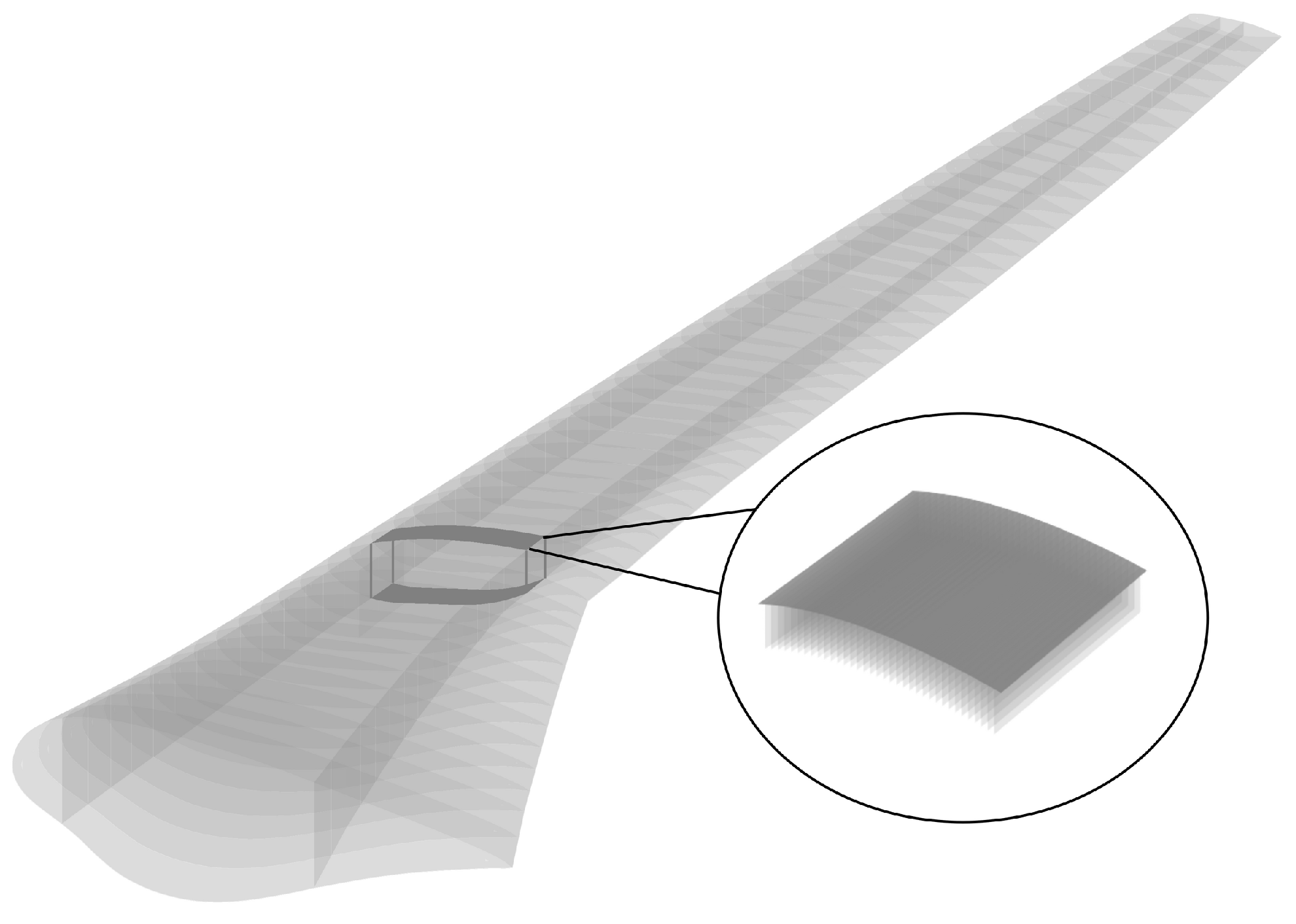
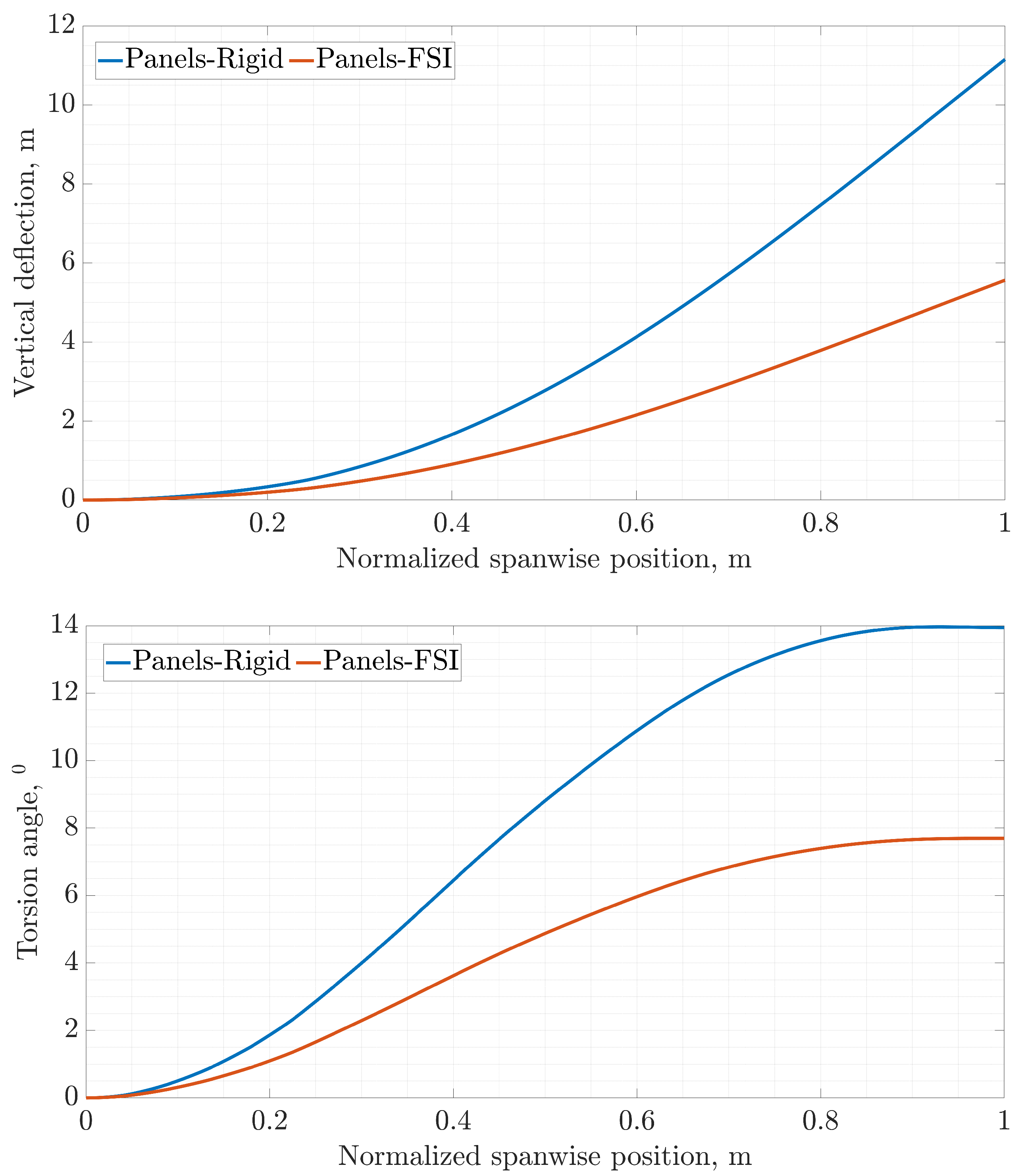
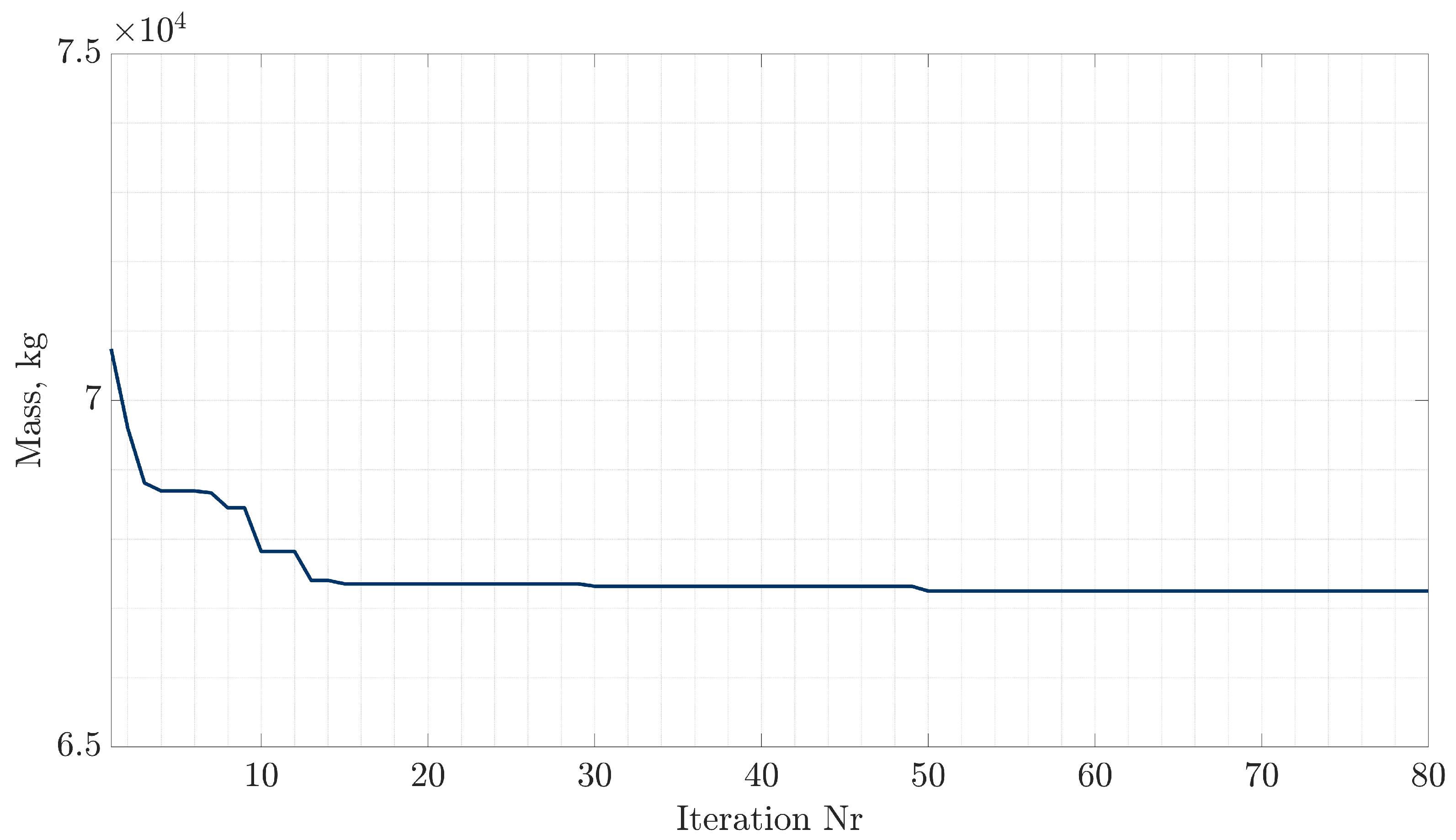
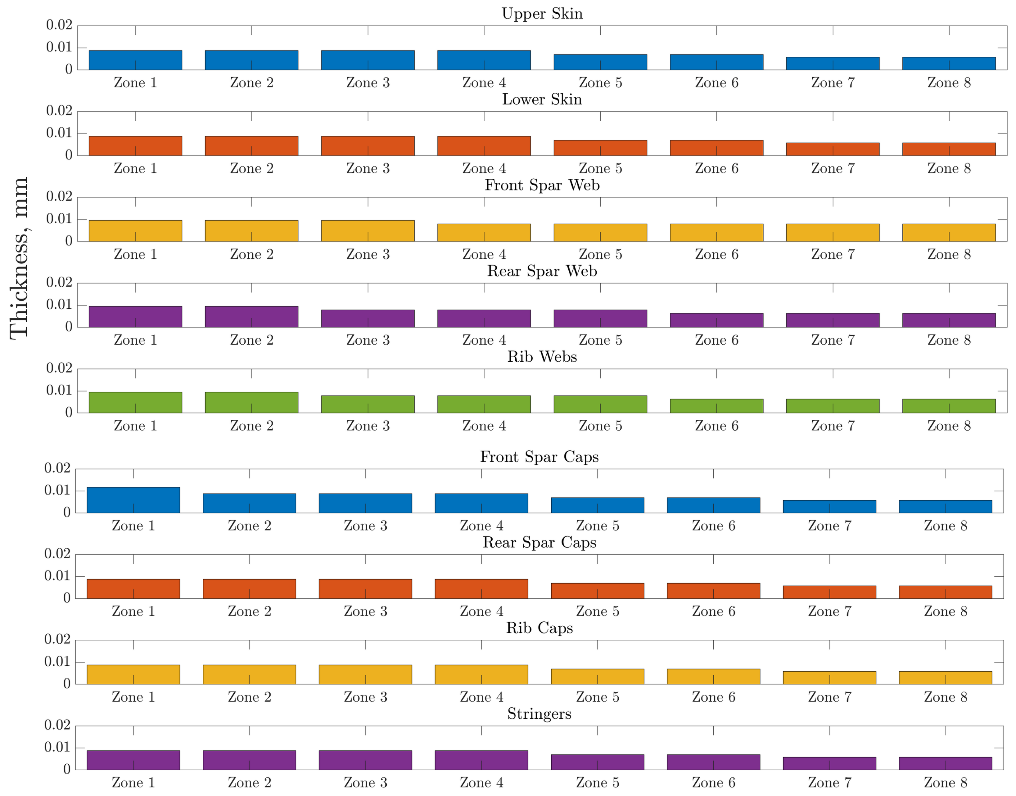
The methodology starts with the main case study and the corresponding 3D FEM model. A sensitivity analysis for the URF value present in the FSI analysis indicated an optimum value of 0.5 for the current case study and critical aerodynamic loading scenario. The bending–torsion coupling allows for a great reduction in the effective AoA, which cascades into lower displacements and overall load reduction, in comparison with rigid aerodynamics. Aiming at providing a step towards the inclusion of the static aeroelastic response early in the design stage at a reduced-as-much-as-possible computational cost, an SBO framework was also provided. In order to increase the efficiency of the framework, the number of design variables was drastically reduced by implementing predefined laminates as well as a thickness distribution for each component of the wing. The SBO framework was then used to drive the mass of the wing to a minimum while satisfying strength, local panel buckling and flutter constraints under the application of the critical aerodynamic loading corresponding to a 2.5 g maneuver. Optimal thickness distributions for each component were obtained. Among the constraints, the buckling critical loads were nearly active at the obtained optimal design, indicating that this type of wing structure might be susceptible to buckling. Strength and flutter constraints were less active in the optimal design. Nevertheless, the NASTRAN flutter solver indicates a dynamic aeroelastic instability, which might need further investigation via higher fidelity methods. Regarding the variables, zones near the yehudi break were accompanied by an increase in thickness. This particular trend was observed for the upper and lower skins and spar caps, since they contribute more to the overall load-carrying capability of the structure.

Several features can be added to the SBO optimization framework presented in this study, in order to obtain more holistic design and optimization methodologies. Both the conceptual and preliminary frameworks could be greatly benefited by the addition of aerodynamic shape optimization procedures. For the composite parts of the wing presented herein, the addition of a library of materials and lay-ups in order could support decision making in manufacturing and cost analysis to a greater extent. A wider variety of global–local analysis techniques, such as the one presented earlier, for the spars buckling, presence of holes and rivets, etc., could enhance cost estimation and manufacturing capabilities, since more light is shed on the detailed design stage.

Last but not least, and as mentioned earlier, the validity and efficiency of the proposed methodology could be enriched by the embodiment of high-fidelity CFD aeroelastic simulations in terms of aerodynamics. Such analyses could be used within a multi-fidelity optimization approach featuring only aeroelastic simulations, since, for at least the current reference wing configuration, great mass and performance gains are expected, as demonstrated.

References

1. Airbus. Global Market Forecast—Cities, Airports & Aircraft 2019–2038; Technical Report; Airbus S.A.S.: Leiden, The Netherlands, 2018. [Google Scholar]
2. Boeing. Boeing Market Outlook; Boeing Commercial Airplanes; Technical Report; The Boeing Company: Arlington, VA, USA, 2018. [Google Scholar]
3. ACARE. ACARE Flightpath 2050—Europe’s Vision for Aviation; Technical Report; Advisory Council for Aviation Research and Innovation in Europe: Brussels, Belgium, 2011. [Google Scholar]
4. Castellani, M.; Cooper, J.E.; Lemmens, Y. Nonlinear Static Aeroelasticity of High-Aspect-Ratio-Wing Aircraft by Finite Element and Multibody Methods. J. Aircr. 2017, 54, 548–560. [Google Scholar] [CrossRef] [Green Version]
5. Roeseler, W.G.; Sarh, B.; Kismarton, M.U. Composite Structures: The First 100 Years. In Proceedings of the 16th Internationnal Conference on Composite Materials; Japan Society for Composite Materials: Kyoto, Japan, 2007. [Google Scholar]
6. Kundu, A.K. Aircraft Design; Cambridge University Press: Cambridge, UK, 2009. [Google Scholar] [CrossRef]
7. Rizzi, A. Modeling and simulating aircraft stability and control—The SimSAC project. Prog. Aerosp. Sci. 2011, 47, 573–588. [Google Scholar] [CrossRef]
8. Triplett, W.E. Aeroelastic Tailoring Studies in Fighter Aircraft Design. J. Aircr. 1980, 17, 508–513. [Google Scholar] [CrossRef]
9. Love, M.; Bohlman, J. Aeroelastic Tailoring Studies in Fighter Aircraft Design; Technical Report; NASA Langley Research Center: Washington, DC, USA, 1989. [Google Scholar]
10. Haftka, R.T. Automated Procedure for Design of Wing Structures to Satisfy Strength and Flutter Requirements; Technical Report; NASA Langley Research Center: Washington, DC, USA, 1973. [Google Scholar]
11. Haftka, R.T. Optimization of flexible wing structures subject to strength and induced drag constraints. AIAA J. 1977, 15, 1101–1106. [Google Scholar] [CrossRef]
12. Jasa, J.P.; Hwang, J.T.; Martins, J.R.R.A. Open-source coupled aerostructural optimization using Python. Struct. Multidiscip. Optim. 2018, 57, 1815–1827. [Google Scholar] [CrossRef]
13. Grozdanov, A. Transonic Static Aeroelasticity Using the 2.5D Nonlinear Vortex Lattice Method. Master’s Thesis, Ecole Polytechnique De Montreal, Montreal, QC, Canada, 2017. [Google Scholar]
14. Schuster, D.M.; Liu, D.D.; Huttsell, L.J. Computational Aeroelasticity: Success, Progress, Challenge. J. Aircr. 2003, 40, 843–856. [Google Scholar] [CrossRef] [Green Version]
15. Smith, M.; Patil, M.; Hodges, D. CFD-based analysis of nonlinear aeroelastic behavior of high-aspect ratio wings. In Proceedings of the 19th AIAA Applied Aerodynamics Conference, Seattle, WA, USA, 16–19 April 2001. [Google Scholar] [CrossRef]
16. Vidanović, N.; Rašuo, B.; Kastratović, G.; Maksimović, S.; Ćurčić, D.; Samardžić, M. Aerodynamic–structural missile fin optimization. Aerosp. Sci. Technol. 2017, 65, 26–45. [Google Scholar] [CrossRef]
17. Brooks, T.R.; Martins, J.R.; Kennedy, G.J. High-fidelity aerostructural optimization of tow-steered composite wings. J. Fluids Struct. 2019, 88, 122–147. [Google Scholar] [CrossRef]
18. Brooks, T.R.; Martins, J.R.R.A.; Kennedy, G.J. Aerostructural Tradeoffs for Tow-Steered Composite Wings. J. Aircr. 2020, 57, 787–799. [Google Scholar] [CrossRef]
19. Kenway, G.; Kennedy, G.; Martins, J.R.R.A. A CAD-Free Approach to High-Fidelity Aerostructural Optimization. In Proceedings of the 13th AIAA/ISSMO Multidisciplinary Analysis Optimization Conference, Fort Worth, TX, USA, 13–15 September 2010; American Institute of Aeronautics and Astronautics: Reston, VA, USA, 2010. [Google Scholar] [CrossRef] [Green Version]
20. Afonso, F.; Vale, J.; Oliveira, É.; Lau, F.; Suleman, A. A review on non-linear aeroelasticity of high aspect-ratio wings. Prog. Aerosp. Sci. 2017, 89, 40–57. [Google Scholar] [CrossRef]
21. Cavagna, L.; Quaranta, G.; Mantegazza, P. Application of Navier–Stokes simulations for aeroelastic stability assessment in transonic regime. Comput. Struct. 2007, 85, 818–832. [Google Scholar] [CrossRef]
22. Crovato, A.; Almeida, H.S.; Vio, G.; Silva, G.H.; Prado, A.P.; Breviglieri, C.; Guner, H.; Cabral, P.H.; Boman, R.; Terrapon, V.E.; et al. Effect of Levels of Fidelity on Steady Aerodynamic and Static Aeroelastic Computations. Aerospace 2020, 7, 42. [Google Scholar] [CrossRef]
23. Kafkas, A.; Kilimtzidis, S.; Kotzakolios, A.; Kostopoulos, V.; Lampeas, G. Multi-Fidelity Optimization of a Composite Airliner Wing Subject to Structural and Aeroelastic Constraints. Aerospace 2021, 8, 398. [Google Scholar] [CrossRef]
24. Martins, J.R.R.A.; Ning, A. Engineering Design Optimization; Cambridge University Press: Cambridge, UK, 2021. [Google Scholar] [CrossRef]
25. Jones, D.R. A Taxonomy of Global Optimization Methods Based on Response Surfaces. J. Glob. Optim. 2001, 21, 345–383. [Google Scholar] [CrossRef]
26. Forrester, A.I.J.; Sóbester, A.; Keane, A.J. Engineering Design via Surrogate Modelling; Wiley: Hoboken, NJ, USA, 2008. [Google Scholar] [CrossRef]
27. Bordogna, M.T.; Bettebghor, D.; Blondeau, C.; de Breuker, R. Surrogate-based aerodynamics for composite wing box sizing. In Proceedings of the 17th International Forum on Aeroelasticity and Structural Dynamics, Como, Italy, 25–28 June 2017. [Google Scholar]
28. Kontogiannis, S.G.; Savill, M.A. A generalized methodology for multidisciplinary design optimization using surrogate modelling and multifidelity analysis. Optim. Eng. 2020, 21, 723–759. [Google Scholar] [CrossRef]
29. Bouhlel, M.A.; He, S.; Martins, J.R.R.A. Scalable gradient–enhanced artificial neural networks for airfoil shape design in the subsonic and transonic regimes. Struct. Multidiscip. Optim. 2020, 61, 1363–1376. [Google Scholar] [CrossRef]
30. Du, X.; He, P.; Martins, J.R. Rapid airfoil design optimization via neural networks-based parameterization and surrogate modeling. Aerosp. Sci. Technol. 2021, 113, 106701. [Google Scholar] [CrossRef]
31. Katz, J.; Plotkin, A. Low-Speed Aerodynamics; Cambridge University Press: Cambridge, UK, 2001. [Google Scholar] [CrossRef]
32. Schmitt, V.; Charpin, F. Pressure Distributions on the ONERA-M6-Wing at Transonic Mach Numbers; Technical Report; Advisory Group for Aerospace Research and Development, North Atlantic Treaty Organization: Washington, DC, USA, 1979. [Google Scholar]
33. Barcelos, M.; Bavestrello, H.; Maute, K. A Schur–Newton–Krylov solver for steady-state aeroelastic analysis and design sensitivity analysis. Comput. Methods Appl. Mech. Eng. 2006, 195, 2050–2069. [Google Scholar] [CrossRef]
34. Küttler, U.; Wall, W.A. Fixed-point fluid–structure interaction solvers with dynamic relaxation. Comput. Mech. 2008, 43, 61–72. [Google Scholar] [CrossRef]
35. Jovanov, K.; Breuker, R.D. Accelerated convergence of static aeroelasticity using low-fidelity aerodynamics. In Proceedings of the 56th AIAA/ASCE/AHS/ASC Structures, Structural Dynamics, and Materials Conference, Kissimmee, FL, USA, 5–9 January 2015; American Institute of Aeronautics and Astronautics: Reston, VA, USA, 2015. [Google Scholar] [CrossRef]
36. Albano, E.; Rodden, W.P. A doublet-lattice method for calculating lift distributions on oscillating surfaces in subsonic flows. AIAA J. 1969, 7, 279–285. [Google Scholar] [CrossRef]
37. Blair, M. A Compilation of the Mathematics Leading to The Doublet Lattice Method; Technical Report; Airforce Wright Laboratory: Austin, TX, USA, 1992. [Google Scholar]
38. Harder, R.L.; Desmarais, R.N. Interpolation using surface splines. J. Aircr. 1972, 9, 189–191. [Google Scholar] [CrossRef]
39. Alexandrov, N.M.; Dennis, J.E.; Lewis, R.M.; Torczon, V. A trust-region framework for managing the use of approximation models in optimization. Struct. Optim. 1998, 15, 16–23. [Google Scholar] [CrossRef]
40. McKay, M.D.; Beckman, R.J.; Conover, W.J. Comparison of Three Methods for Selecting Values of Input Variables in the Analysis of Output from a Computer Code. Technometrics 1979, 21, 239–245. [Google Scholar] [CrossRef]
41. Jones, R.M. Mechanics of Composite Materials; CRC Press: Boca Raton, FL, USA, 2018. [Google Scholar] [CrossRef]
42. Tsai, S.W.; Hahn, H.T. Introduction to Composite Materials; Routledge: Milton Park, UK, 2018. [Google Scholar] [CrossRef]
43. Kreisselmeier, G.; Steinhauser, R. Systematic Control Design by Optimizing a Vector Performance Index. IFAC Proc. Vol. 1979, 12, 113–117. [Google Scholar] [CrossRef]
44. Poon, N.M.K.; Martins, J.R.R.A. An adaptive approach to constraint aggregation using adjoint sensitivity analysis. Struct. Multidiscip. Optim. 2006, 34, 61–73. [Google Scholar] [CrossRef]
45. Lambe, A.B.; Kennedy, G.J.; Martins, J.R.R.A. An evaluation of constraint aggregation strategies for wing box mass minimization. Struct. Multidiscip. Optim. 2016, 55, 257–277. [Google Scholar] [CrossRef]
46. Lambe, A.B.; Martins, J.R.R.A. Matrix-free aerostructural optimization of aircraft wings. Struct. Multidiscip. Optim. 2015, 53, 589–603. [Google Scholar] [CrossRef]
47. Dababneh, O. Multidisciplinary Design Optimisation for Aircraft Wing Mass Estimation. Ph.D. Thesis, Cranfield University, Bedford, UK, 2016. [Google Scholar]
48. Kassapoglou, C. Design and Analysis of Composite Structures; John Wiley & Sons Ltd.: Hoboken, NJ, USA, 2013. [Google Scholar] [CrossRef]
49. Vassberg, J.; Dehaan, M.; Rivers, M.; Wahls, R. Development of a Common Research Model for Applied CFD Validation Studies. In Proceedings of the 26th AIAA Applied Aerodynamics Conference, Honolulu, HI, USA, 18–21 August 2008; American Institute of Aeronautics and Astronautics: Reston, VA, USA, 2008. [Google Scholar] [CrossRef] [Green Version]
50. Brooks, T.R.; Kenway, G.K.W.; Martins, J.R.R.A. Benchmark Aerostructural Models for the Study of Transonic Aircraft Wings. AIAA J. 2018, 56, 2840–2855. [Google Scholar] [CrossRef]
51. Marlett, K. HEXCEL 8552 IM7 Unidirectional Prepreg 190 gsm 35% RC Qualification Statistical Analysis Report, Rept. NCP-RP-2009-028 Rev B; Technical Report; National Institute for Aviation Research: Wichita, KS, USA, 2011. [Google Scholar]
52. Marlett, K. HEXCEL 8552S AS4 Plain Weave Fabric 193 gsm 38% RC Qualification Material Property Data Report, Rept. CAM-RP-2010-006 N/C; Technical Report; National Institute for Aviation Research: Wichita, KS, USA, 2011. [Google Scholar]
53. Gray, A.C. Geometrically Nonlinear High Fidelity Aerostructural Optimisation for Highly Flexible Wings. Master’s Thesis, Delft University of Technology, Delft, The Netherlands, 2021. [Google Scholar]
54. Wright, J.R.; Cooper, J.E. Introduction to Aircraft Aeroelasticity and Loads; Wiley: Hoboken, NJ, USA, 2014. [Google Scholar] [CrossRef]
55. Brazier, L.G. On the flexure of thin cylindrical shells and other “thin” sections. Proc. R. Soc. A Math. Phys. Eng. Sci. 1927, 116, 104–114. [Google Scholar] [CrossRef] [Green Version]
56. Lee, S.H. MSC/NASTRAN Nonlinear Analysis Handbook Version 67; MacNeal-Schwendler Corp.: Los Angeles, CA, USA, 1992. [Google Scholar]
Figure 1. 3D-panel-method staggered FSI scheme.
Aerospace 10 00251 g001
Figure 2. DLM aerodynamics model of the main case study.
Aerospace 10 00251 g002
Figure 3. FEM structural nodes used for aerodynamic-loads interpolation purposes.
Aerospace 10 00251 g003
Figure 4. Global–local modeling approach.
Aerospace 10 00251 g004
Figure 5. Optimization zones for the SBO framework.
Aerospace 10 00251 g005
Figure 6. Flowchart of the SBO framework.
Aerospace 10 00251 g006
Figure 7. uCRM13.5 internal configuration and OML.
Aerospace 10 00251 g007
Figure 8. uCRM13.5 wing FEM mesh and fuel distribution detail.
Aerospace 10 00251 g008
Figure 9. Displacements and lift coefficient convergence characteristics for a URF value of 0.5.
Aerospace 10 00251 g009
Figure 10. Deflection and torsion angle comparison between rigid and elastic aerodynamics for the uCRM-13.5 wing.
Aerospace 10 00251 g010
Figure 11. Deflection, torsion angle and tip shortening comparison between linear and nonlinear structural response of the uCRM-13.5 wing.
Aerospace 10 00251 g011
Figure 12. Convergence of the objective function.
Aerospace 10 00251 g012
Figure 13. Convergence of the L1-norm of the constraints violation.
Aerospace 10 00251 g013
Figure 14. SBO optimal design—spanwise thickness distribution per component.
Aerospace 10 00251 g014
Figure 15. SBO thickness reduction at each part and zone of the reference wing.
Aerospace 10 00251 g015
Figure 16. SBO optimal design—deflected shape.
Aerospace 10 00251 g016
Figure 17. SBO optimal design—maximum FI at each laminate.
Aerospace 10 00251 g017