Control of Electromagnetic Formation Flight of Two Satellites in Low Earth Orbits

Abstract

Electromagnetic formation flight uses the electromagnetic interaction between satellites to provide maneuver control for formation satellites, with the advantages of no propellant consumption, long life, and high flexibility. However, high-precision control for electromagnetic formation flight is challenging because of the nonlinear and coupling characteristics of the dynamics, optimal assignment of magnetic dipoles, model uncertainties, and the angular momentum management issues caused by the geomagnetic field. This paper studies the 6-DOF control problem of two-satellite electromagnetic formation flight in low-Earth orbit. A new electromagnetic frame is introduced to promote the decoupling of the translation dynamics model and the electromagnetic model. The electromagnetic model can be expressed as a simple two-dimensional model in this electromagnetic frame. The proposed electromagnetic force envelope diagram can intuitively show the relationship between electromagnetic force and magnetic dipoles, providing practical guidance for dipole assignment. The frequency division multiplexing method is designed for angular momentum management considering the effect of the earth’s magnetic field on the electromagnetic satellites, and the active disturbance rejection control method is used to solve the 6-DOF stability problem with external disturbance and model uncertainties. Numerical simulation verifies the effectiveness of the proposed control method and angular momentum management strategy.

1. Introduction

With the development of technology, the functions of satellites have been continuously enhanced [1,2] to meet more and more space mission requirements. In particular, satellite formation technology [3] has opened up a new space for the application of small satellites. Satellite formation refers to the close cooperative movement of multiple satellites in a specific configuration, which has broad application prospects in earth observation, astronomical observation, and deep space exploration. However, accurate formation configuration maintenance requires frequent maneuver control. Traditional thrusters consume a lot of propellant and cause plume pollution, and the mission life of formation flight is restricted by the available propellant.

Electromagnetic formation flight (EMFF) has attracted extensive attention as a formation flying technology without propellant consumption [4,5]. The operational principle of EMFF is that each satellite is equipped with electromagnetic coils equivalent to a magnetic dipole, and the interaction between magnetic dipoles generates electromagnetic force and electromagnetic torque to control the relative motion of the satellites. The inter-satellite electromagnetic force has the advantages of non-contact and continuous adjustment, and its feasible interaction range is tens to hundreds of meters [6]. However, the nonlinearity and coupling of electromagnetic force/torque, the uncertainties of the electromagnetic model and inertia moment of the satellites, the effect of the geomagnetic field on electromagnetic satellites, and the high-precision control requirements of space missions on formation satellites pose challenges to the dynamic modeling and controller design of EMFF.

The 6-DOF dynamic modeling of EMFF usually decouples the relative position and attitude. The inter-satellite electromagnetic force controls the relative translational motion of the satellite. Each satellite is equipped with reaction wheels to control the satellite’s attitude [7]. The electromagnetic torque is treated as the disturbance torque. The electromagnetic frame is introduced to decouple the relative translational dynamics model and the electromagnetic model to reduce the nonlinearity of the translational dynamics model. The electromagnetic frame is obtained by rotating the orbital coordinate system several times, and the relative position coordinates of the satellites determine the rotation angle [8]. However, the problem caused by the above electromagnetic frame is that the rotation angle may appear singular in some cases. In addition, when the 3D electromagnetic model is used to solve the magnetic dipole with a given electromagnetic force profile, it is challenging to allocate and optimize the magnetic dipoles in real time due to the nonlinearity and coupling of the far-field electromagnetic model. Some studies discussed the optimization problem of magnetic dipoles to minimize the energy consumption of the electromagnetic coil or the angular momentum of the reaction wheel [9,10,11,12,13]. Huang [9] introduced the dipole parameter to represent relations between electromagnetic force and torque, sought the analytical dipole solution to minimize the electromagnetic torque, and optimized the angular momentum based on sliding mode control. Schweigheart [10,11] proposed the homotopy method to solve the magnetic dipoles for the multi-satellite formation and used the effective set method and gradient projection method to optimize the dipoles. However, these methods are mainly based on numerical optimization and rely on the initial value of the dipoles. If the initial value is set unreasonably, the dipoles’ magnitude will differ among different satellites. In addition, the dipoles cannot be optimized online. We propose the electromagnetic frame construction method based on energy optimization constraints to solve the above problems. The realization of the coordinate transformation between the electromagnetic coordinate system and the orbital coordinate system does not require a transformation matrix. In addition, the electromagnetic model can be expressed as the two-dimensional model in this electromagnetic frame, significantly reducing the nonlinearity and coupling. The proposed envelope diagram of the electromagnetic force can intuitively show the relationship between the electromagnetic force and the dipoles. According to the electromagnetic force envelope, we give the analytical dipole solutions for the two optimization objectives of energy optimization and dipole differentiability.

For EMFF in low earth orbit, the Earth’s strong magnetic field will produce considerable disturbance torque on the satellite, and angular momentum management may be a problem. The polarity reversal method proposed in [14,15] refers to simultaneously changing all satellites’ magnetic dipoles’ signs. At this time, the direction of the disturbance torque of the geomagnetic field on satellites varies to unload the angular momentum, while the electromagnetic force between satellites remains unchanged. The frequency division multiplexing (FDM) technique proposed in [16,17,18] refers to modulating the electromagnetic coil current of satellites with periodical carriers, and the carrier frequency is much higher than the formation orbit frequency. The advantage of the FDM method is that the average value of the disturbance torque on each satellite caused by the Earth’s magnetic field in a modulation period is almost zero. The FDM method produces effective control but also brings transient residual electromagnetic force. We use a simple form of carrier current to modulate the magnetic dipoles, and the residual electromagnetic force can be treated as a real-time disturbance.

External disturbance force/moment, inertia matrix uncertainty, and coupled nonlinear terms are considered uncertain parts of the satellite attitude and orbit control system [19]. In addition, considering the electromagnetic model’s uncertainty and actuators’ saturation is also very necessary to study EMFF. Achieving high-precision formation control performance in the presence of the above issues is challenging. Some scholars have researched control methods of EMFF, such as adaptive control [7,14], sliding mode control [15,20], linear quadratic regulation (LQR) control [21,22], and robust suboptimal control [12]. Due to the strong nonlinearity and coupling of EMFF dynamics, most controllers need to rely on accurate dynamics models to achieve high-precision control of EMFF. However, the active disturbance rejection controller (ADRC) is a robust control method that does not need to rely on the dynamics model. It can estimate and compensate for the external disturbance and the model uncertainty of the system online. Ref. [23] discussed the estimation uncertainty ability of the extended state observer (ESO), the core component of ADRC, and gave the observable disturbance range of ESO under bounded observation error. In recent years, ADRC has been widely used in many fields [24]. However, ADRC is rarely used in EMFF. We propose an ADRC controller for 6-DOF EMFF and analyze the influence of continuity and differentiability of magnetic dipoles on ESO observation error for improving the system control accuracy.

This paper analyzes the dynamic characteristics of the two-satellite EMFF, discusses the problem of magnetic dipole assignment, and proposes the 6-DOF control of EMFF based on the active disturbance rejection control (ADRC) framework considering the angular momentum management strategy of the polarity reversal and the frequency division. The contributions of this paper are summarized as follows:

• An electromagnetic frame construction method based on energy optimization constraint is proposed, which simplifies the orbital frame and the electromagnetic frame relation, and realizes coordinate system transformation without using the transformation matrix.
• To reasonably assign the magnetic dipoles, the relationship diagram between the electromagnetic force envelope and the magnetic dipoles is established, and the magnetic dipole solutions with optimal energy and differentiable dipoles are given. In addition, the differentiable magnetic dipoles can ensure the differentiability of the disturbance torque of the geomagnetic field on the satellite, which is conducive to reducing the observation error of ESO.
• The frequency division method is proposed to aim at the angular momentum management problem. The carrier current is simple in form, without phase modulation. The alternating part of the generated electromagnetic force is treated as an external disturbance. ADRC estimates and compensates for the system’s model uncertainties and external disturbance in real time.

The remainder of this paper is organized as follows. Section 2 introduces the dynamic model of the two-satellite electromagnetic formation. Section 3 proposes the magnetic dipoles allocation methods and angular momentum management strategies. Section 4 presents the translational and attitude control of the two-satellite formation based on ADRC. The numerical simulation results are discussed in Section 5. Finally, some useful conclusions are given.

2. Dynamic Model

2.1. Coordinate System

The coordinate system used in this paper is shown in Figure 1, where $O_{\mathrm{E}}XYZ$ is the Earth Central Inertial (ECI) Frame; $O_{\mathrm{CM}}{x}_{\mathrm{CM}}{y}_{\mathrm{CM}}{z}_{\mathrm{CM}}$ is the orbital frame, and its origin is located at the center of mass of the formation (recorded as $O_{\mathrm{CM}}$), ${\mathit{O}}_{\mathrm{CM}}{\mathit{x}}_{\mathrm{CM}}$ points the direction from the earth center to the formation center of mass, ${\mathit{O}}_{\mathrm{CM}}{\mathit{z}}_{\mathrm{CM}}$ points towards the orbital plane normal, and ${\mathit{O}}_{\mathrm{CM}}{\mathit{y}}_{\mathrm{CM}}$ constitutes the right-hand system. $O_A^{\mathrm{b}}{x}_A^{\mathrm{b}}{y}_A^{\mathrm{b}}{z}_A^{\mathrm{b}}$ and $O_B^{\mathrm{b}}{x}_B^{\mathrm{b}}{y}_B^{\mathrm{b}}{z}_B^{\mathrm{b}}$ are the body-fixed frames of satellites A and B, respectively, and their coordinate axes are aligned with the principal inertia axis of the satellites. In addition, $O_{\mathrm{CM}}{x}_{\mathrm{EM}}{y}_{\mathrm{EM}}{z}_{\mathrm{EM}}$ is the electromagnetic coordinate frame. $O_{\mathrm{CM}}{x}_{\mathrm{EM}}$ is pointing from satellite A to satellite B. ${\mathit{O}}_{\mathrm{CM}}{\mathit{y}}_{\mathrm{EM}}$ is located on the plane formed by the electromagnetic force $\mathit{F}$ and ${\mathit{O}}_{\mathrm{CM}}{\mathit{x}}_{\mathrm{EM}}$, and the component of $\mathit{F}$ decomposed in the ${\mathit{O}}_{\mathrm{CM}}{\mathit{y}}_{\mathrm{EM}}$ direction is positive. ${\mathit{O}}_{\mathrm{CM}}{\mathit{z}}_{\mathrm{EM}}$ completes the right-hand system. The component of $\mathit{F}$ decomposed in the ${\mathit{O}}_{\mathrm{CM}}{\mathit{z}}_{\mathrm{EM}}$ direction is zero. When the electromagnetic force is parallel to the ${\mathit{O}}_{\mathrm{CM}}{\mathit{x}}_{\mathrm{EM}}$ direction, the electromagnetic force decomposed in the ${\mathit{O}}_{\mathrm{CM}}{\mathit{y}}_{\mathrm{EM}}$ direction is also zero.

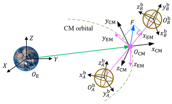
Figure 1. Reference frames.

The rotation matrices that rotate ${\varphi }_x$, ${\varphi }_y$, and ${\varphi }_z$ around the coordinate system’s x, y, and z axes are expressed as

$${\mathit{R}}_x\left({\varphi }_x\right)=\left[\begin{array}{ccc}1& 0& 0\\ 0& \cos {\varphi }_x& -\sin {\varphi }_x\\ 0& \sin {\varphi }_x& \cos {\varphi }_x\end{array}\right],{\mathit{R}}_y\left({\varphi }_y\right)=\left[\begin{array}{ccc}\cos {\varphi }_y& 0& \sin {\varphi }_y\\ 0& 1& 0\\ -\sin {\varphi }_y& 0& \cos {\varphi }_y\end{array}\right],{\mathit{R}}_z\left({\varphi }_z\right)=\left[\begin{array}{ccc}\cos {\varphi }_z& -\sin {\varphi }_z& 0\\ \sin {\varphi }_z& \cos {\varphi }_z& 0\\ 0& 0& 1\end{array}\right]$$

(1)

The transformation matrix [13] from $O_{\mathrm{E}}XYZ$ to $O_{\mathrm{CM}}{x}_{\mathrm{CM}}{y}_{\mathrm{CM}}{z}_{\mathrm{CM}}$ can be expressed as

$${}^{\mathrm{CM}}\mathit{T}^{\mathrm{ECI}}={\mathit{R}}_z\left(u\right){\mathit{R}}_x\left(i\right){\mathit{R}}_z\left(\Omega \right)$$

(2)

where $i$ is the orbital inclination, $\Omega$ is the right ascension of ascending node, $u=u_0+{\omega }_{\mathrm{CM}}t$ is the argument of latitude, $u_0$ is the argument of latitude at time $t=0$, and ${\omega }_{\mathrm{CM}}$ is the orbital angular velocity of the center of mass of the formation.

The relative position vector of two satellites is expressed as ${\mathit{\rho }}^{\mathrm{CM}}={\left[\begin{array}{ccc}x& y& z\end{array}\right]}^{\mathrm{T}}$ in the orbital frame, while the position is recorded as ${\mathit{\rho }}^{\mathrm{EM}}={\left[\begin{array}{ccc}d& 0& 0\end{array}\right]}^{\mathrm{T}}$ in the electromagnetic frame. The electromagnetic force is recorded as ${\mathit{F}}^{\mathrm{CM}}$ in the orbital frame and ${\mathit{F}}^{\mathrm{EM}}$ in the electromagnetic frame. The angle between ${\mathit{F}}^{\mathrm{CM}}$ and ${\mathit{\rho }}^{\mathrm{CM}}$ is defined as $\left(\pi -\gamma \right)$, where $\gamma \in \left[0,\pi \right]$. The parameters have the following relationships.

$$\left\{\begin{array}{l}\gamma =\arccos \left(-{\hat{\mathit{F}}}^{\mathrm{CM}}\cdot {\hat{\mathit{\rho }}}^{\mathrm{CM}}\right)\\ {\mathit{F}}^{\mathrm{EM}}=‖{\mathit{F}}^{\mathrm{CM}}‖{\left[-\cos \gamma \hspace{1em}\sin \gamma \hspace{1em}0\right]}^{\mathrm{T}}\end{array}\right.$$

(3)

where ${\hat{\mathit{F}}}^{\mathrm{CM}}$ represents the unit vector of ${\mathit{F}}^{\mathrm{CM}}$, and ${\hat{\mathit{\rho }}}^{\mathrm{CM}}$ represents the unit vector of the relative position of the two satellites in the orbital frame.

2.2. Electromagnetic Model

The three-dimensional orthogonal coils installed on the satellite can be equivalent to a magnetic dipole. Because the z-axis component of the electromagnetic force in the electromagnetic frame is 0, the magnetic dipoles of the two satellites can be designed to be on the plane ${\mathit{x}}_{\mathrm{EM}}{\mathit{O}}_{\mathrm{CM}}{\mathit{y}}_{\mathrm{EM}}$ in the electromagnetic frame. The electromagnetic frame is shown in Figure 2. ${\mathit{\mu }}_A$ and ${\mathit{\mu }}_B$ represent the magnetic dipoles of satellite A and satellite B, $d$ is the distance between the centers of the two dipoles, $\left(\alpha ,\beta \right)$ are the included angles between the direction of the magnetic dipoles and ${\mathit{O}}_{\mathrm{CM}}{\mathit{x}}_{\mathrm{EM}}$.

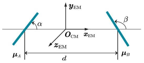
Figure 2. Electromagnetic frame.

In the electromagnetic coordinate system, the magnetic dipoles can be expressed as

$$\left\{\begin{array}{ll}{\mathit{\mu }}_A& ={\mu }_A{\left[\cos \alpha \hspace{1em}\sin \alpha \hspace{1em}0\right]}^{\mathrm{T}}\\ {\mathit{\mu }}_B& ={\mu }_B{\left[\cos \beta \hspace{1em}\sin \beta \hspace{1em}0\right]}^{\mathrm{T}}\end{array}\right.$$

(4)

According to the electromagnetic far-field model [8], the inter-satellite electromagnetic force and torque are expressed as

$$\begin{array}{l}\left\{\begin{array}{l}{\mathit{F}}^{\mathrm{EM}}=A_0{\left[-\left(3\cos m+\cos n\right)2\sin m\hspace{1em}0\right]}^{\mathrm{T}}\\ {\mathit{\tau }}_A=A_1{\left[0\hspace{1em}0\hspace{1em}3\sin m+\sin n\right]}^{\mathrm{T}}\\ {\mathit{\tau }}_B=A_1{\left[0\hspace{1em}0\hspace{1em}3\sin m-\sin n\right]}^{\mathrm{T}}\end{array}\right.\\ \left\{\begin{array}{l}{\mathit{F}}^{\mathrm{EM}}=A_0{\left[-\left(3\cos m+\cos n\right)\hspace{1em}2\sin m\hspace{1em}0\right]}^{\mathrm{T}}\\ {\mathit{\tau }}_A=A_1{\left[0\hspace{1em}0\hspace{1em}3\sin m+\sin n\right]}^{\mathrm{T}}\\ {\mathit{\tau }}_B=A_1{\left[0\hspace{1em}0\hspace{1em}3\sin m-\sin n\right]}^{\mathrm{T}}\end{array}\right.\end{array}$$

(5)

where ${\mu }_0=4\pi \times {10}^{-7}\mathrm{N}/{\mathrm{A}}^2$ is the permeability of free space, $A_0=\frac{3{\mu }_0}{8\pi }\frac{{\mu }_A\cdot {\mu }_B}{d^4}$, $A_1=-\frac{{\mu }_0}{8\pi }\frac{{\mu }_A\cdot {\mu }_B}{d^3}$, $m=\alpha +\beta$, and $n=\alpha -\beta$. Equation (5) can quickly solve and optimize the magnetic dipoles. In addition, the magnetic dipoles can also be easily represented in the orbital frame. Take satellite A as an example, and the relationship is as follows.

$${\mathit{\mu }}_A^{\mathrm{CM}}=\left\{\begin{array}{l}\frac{{\mu }_A\sin \alpha }{\sin \gamma }{\hat{\mathit{F}}}^{\mathrm{CM}}+{\mu }_A\left(\cos \alpha +\sin \alpha \cot \gamma \right){\hat{\mathit{\rho }}}^{\mathrm{CM}},\gamma \ne 0\hspace{1em}\mathrm{and}\hspace{1em}\gamma \ne \pi \\ {\mu }_A\cdot {\hat{\mathit{\rho }}}^{\mathrm{CM}},\gamma =0\hspace{1em}\mathrm{or}\hspace{1em}\gamma =\pi \end{array}\right.$$

(6)

The electromagnetic torque is expressed as

$${\mathit{\tau }}_A^{\mathrm{CM}}={\mathit{\tau }}_A\left({\hat{\mathit{\rho }}}^{\mathrm{CM}}\times {\hat{\mathit{F}}}^{\mathrm{CM}}\right)$$

(7)

2.3. Relative Translational Dynamics

Denote the masses of satellites A and B are $m_A$ and $m_B$, the position vectors of the two satellites in the orbital frame are noted as ${\mathit{\rho }}_A$ and ${\mathit{\rho }}_B$, respectively, and the relative position vectors of the double satellites are $\mathit{\rho }={\mathit{\rho }}_B-{\mathit{\rho }}_A$. According to the definition of the center of mass of the formation, it has $m_A{\mathit{\rho }}_A+m_B{\mathit{\rho }}_B=0$, then

$${\mathit{\rho }}_A=-\frac{m_B}{m_A+m_B}\mathit{\rho },{\mathit{\rho }}_B=\frac{m_A}{m_A+m_B}\mathit{\rho }$$

(8)

Since the inter-satellite electromagnetic force is the internal force of the system, the electromagnetic force will not change the position of the system center of mass. For the close formation with the center of mass in a circular orbit, the relative dynamic equation of the two-satellite electromagnetic formation can be expressed by the Clohessy–Wiltshire (CW) equation [25]:

$$\left\{\begin{array}{l}\ddot{x}=3{\omega }_0^{2}x+2{\omega }_0\dot{y}+u_x+f_{dx}\\ \ddot{y}=-2{\omega }_0\dot{x}+u_y+f_{dy}\\ \ddot{z}=-{\omega }_0^{2}z+u_z+f_{dz}\end{array}\right.$$

(9)

where ${\omega }_0=\sqrt{\mu /r_{CM}^3}$ is the angular velocity of the system center of mass moving around the earth, $\mu =3.986\times {10}^{14}{\mathrm{m}}^3/{\mathrm{s}}^2$ is the gravity constant of the Earth, $r_{\mathrm{CM}}$ is the distance between the earth’s center and the formation center of mass, $\mathit{u}=\frac{m_A+m_B}{m_A{m}_B}{\mathit{F}}^{\mathrm{CM}}={\left[\begin{array}{ccc}{u}_x& u_y& u_z\end{array}\right]}^{\mathrm{T}}$ is the control acceleration, and ${\mathit{f}}_d={\left[\begin{array}{ccc}{f}_{dx}& f_{dy}& f_{dz}\end{array}\right]}^{\mathrm{T}}$ is the external disturbance acceleration.

2.4. Attitude Dynamics

Unit quaternions can be used to describe rotation. For the frame rotation about a unit axis $\mathit{n}$ with an angle $\left|\theta \right|<2\pi$, there is a unit quaternion

$$\mathit{q}={\left[\begin{array}{cc}\cos \left(\frac{\left|\theta \right|}{2}\right)& \sin \left(\frac{\left|\theta \right|}{2}\right)\mathit{n}\end{array}\right]}^{\mathrm{T}}$$

(10)

The logarithm of a unit quaternion [26] is defined as

$$\ln \mathit{q}=\left[\begin{array}{c}0\\ \mathit{\theta }/2\end{array}\right]$$

(11)

where $\mathit{\theta }=\left|\theta \right|\mathit{n}$ is a vector.

According to [27], $\mathit{q}={\left[\begin{array}{cc}{q}_0& {\mathit{q}}_v^{\mathrm{T}}\end{array}\right]}^{\mathrm{T}}={\left[\begin{array}{cccc}{q}_0& q_1& q_2& q_3\end{array}\right]}^{\mathrm{T}}$ is employed to describe the quaternion of the body fixed frame with respect to the inertial frame. ${\mathit{q}}_v={\left[\begin{array}{ccc}{q}_1& q_2& q_3\end{array}\right]}^{\mathrm{T}}$ is the vector part, $q_0$ is the scalar component, and satisfies the constraint ${\mathit{q}}_v^{\mathrm{T}}{\mathit{q}}_v+q_0^2=1$.

The attitude kinematics and dynamics of rigid spacecraft can be modeled [27] as follows:

$$\begin{array}{l}\dot{\mathit{q}}=\frac{1}{2}\left[\begin{array}{c}-{\mathit{q}}_v^{\mathrm{T}}\\ \left(q_0{\mathit{I}}_3+q_{\mathit{v}}^{\times }\right)\end{array}\right]\mathbf{\Omega }\equiv \frac{1}{2}M\left(\mathit{q}\right)\mathbf{\Omega }\\ \mathit{J}\dot{\mathbf{\Omega }}=-{\mathbf{\Omega }}^{\times }\left(\mathit{J}\mathbf{\Omega }+\mathit{h}\right)-\dot{\mathit{h}}+{\mathit{\tau }}_d\end{array}$$

(12)

where $\mathit{J}$ is the symmetric inertia matrix of the satellite, $\mathbf{\Omega }$ is the angular velocity of the satellite with respect to the ECI frame and expressed in the body frame, $\mathit{h}$ is the total stored angular momentum in the wheels, the term ${\mathbf{\Omega }}^{\times }\left(\mathit{J}\mathbf{\Omega }+\mathit{h}\right)$ corresponds to the effect of the rotation of the body-fixed coordinate system [28]. $\dot{\mathit{h}}={\mathit{\tau }}_{RW}$ is reaction wheel torque, and let ${\mathit{\tau }}_c=-{\mathbf{\Omega }}^{\times }\mathit{h}-\dot{\mathit{h}}$ is the control torque of the system. ${\mathit{\tau }}_d$ is the external unknown disturbance torque, mainly including the electromagnetic torque acting on the satellite by the geomagnetic field and other satellites, and the gravity gradient torque. The long-term external disturbance will cause the angular momentum of the reaction wheel to increase over time, resulting in angular momentum saturation. External torques, such as thrusters or magnetic torque, must unload angular momentum [29]. An equilibrium strategy for attitude control and angular momentum management was proposed in [30]. ${\mathit{I}}_3$ is the $3\times 3$ identity matrix. In addition, for any vector $\mathit{a}={\left[\begin{array}{ccc}{a}_1& a_2& a_3\end{array}\right]}^{\mathrm{T}}$, the cross-product operation is

$${\mathit{a}}^{\times }=\left[\begin{array}{ccc}0& -a_3& a_2\\ a_3& 0& -a_1\\ -a_2& a_1& 0\end{array}\right]$$

(13)

Denote ${\mathit{q}}_d={\left[\begin{array}{cc}{q}_{d0}& {\mathit{q}}_{dv}^{\mathrm{T}}\end{array}\right]}^{\mathrm{T}}$ as the desired attitude of the spacecraft, ${\mathbf{\Omega }}_d$ is the desired angular velocity, and the desired attitude motion is

$${\dot{\mathit{q}}}_d=\frac{1}{2}M\left({\mathit{q}}_d\right){\mathbf{\Omega }}_d$$

(14)

The objective of attitude tracking can be transformed into the stability problem by introducing error quaternion ${\mathit{q}}_e={\left[\begin{array}{cc}{q}_{e0}& {\mathit{q}}_{ev}^{\mathrm{T}}\end{array}\right]}^{\mathrm{T}}$, where ${\mathit{q}}_{ev}={\left[\begin{array}{ccc}{q}_{e1}& q_{e2}& q_{e3}\end{array}\right]}^{\mathrm{T}}$. Denote ${\mathit{q}}_d^{\ast }={\left[\begin{array}{cc}{q}_{d0}& -{\mathit{q}}_{dv}^{\mathrm{T}}\end{array}\right]}^{\mathrm{T}}$ as the conjugate quaternion of ${\mathit{q}}_d$. The error quaternion [27] is expressed as

$$\begin{array}{l}{\mathit{q}}_e={\mathit{q}}_d^{\ast }\circ \mathit{q}=\left[\begin{array}{c}{\mathit{q}}_{dv}^{\mathrm{T}}{\mathit{q}}_v+q_0{q}_{d0}\\ q_{d0}{\mathit{q}}_v-{\mathit{q}}_{dv}^{\times }{\mathit{q}}_v-q_0{\mathit{q}}_{dv}\end{array}\right]\\ \mathit{\omega }=\mathbf{\Omega }-\mathit{C}{\mathbf{\Omega }}_d\end{array}$$

(15)

where “$\circ$” denotes the multiplication operator between the quaternion. $\mathit{C}=\left(q_{e0}^2-{\mathit{q}}_{ev}^{\mathrm{T}}{\mathit{q}}_{ev}\right){\mathit{I}}_3+2{\mathit{q}}_{ev}{\mathit{q}}_{ev}^{\mathrm{T}}-2q_{e0}{\mathit{q}}_{ev}^{\times }$, $‖\mathit{C}‖=1,\dot{\mathit{C}}=-{\mathit{\omega }}^{\times }\mathit{C}$. Then, it obtains the error dynamics equation [27]:

$$\begin{array}{l}{\dot{\mathit{q}}}_e=\frac{1}{2}M\left({\mathit{q}}_e\right)\mathit{\omega }=\frac{1}{2}\left[\begin{array}{c}-{\mathit{q}}_{ev}^{\mathrm{T}}\\ \left(q_{e0}{\mathit{I}}_3+{\mathit{q}}_{ev}^{\times }\right)\end{array}\right]\mathit{\omega }\\ \mathit{J}\dot{\mathit{\omega }}=-{\left(\mathit{\omega }+\mathit{C}{\mathbf{\Omega }}_d\right)}^{\times }\mathit{J}\left(\mathit{\omega }+\mathit{C}{\mathbf{\Omega }}_d\right)+\mathit{J}\left({\mathit{\omega }}^{\times }\mathit{C}{\mathbf{\Omega }}_d-\mathit{C}{\dot{\mathbf{\Omega }}}_d\right)+{\mathit{\tau }}_c+{\mathit{\tau }}_d\end{array}$$

(16)

2.5. Earth’s Magnetic Field Model

For electromagnetic formations in close range (usually tens to hundreds of meters), the disturbance force that acts on the satellite due to the earth’s magnetic field is far less than the inter-satellite electromagnetic force. In contrast, the disturbance torque acting on the satellite due to the earth’s magnetic field is significant because it is the same order of magnitude or greater than the inter-satellite electromagnetic torque in the low-Earth orbit. Therefore, the disturbance torque caused by the earth’s magnetic field must be eliminated or used in the controller design.

The geomagnetic frame is noted as $O_{\mathrm{E}}{x}_{\mathrm{EMF}}{y}_{\mathrm{EMF}}{z}_{\mathrm{EMF}}$. The geomagnetic field can be assumed to be a magnetic dipole passing through the Earth’s center, with an angle of about 11.2° between the dipole direction and the Earth’s rotation axis [8]. The Earth’s magnetic dipole is oriented along the z-axis in the geomagnetic frame, expressed as ${\mathit{\mu }}_{\mathrm{E}}^{\mathrm{EMF}}={\left[\begin{array}{ccc}0& 0& -{\mu }_e\end{array}\right]}^{\mathrm{T}}$, where ${\mu }_e\approx 8\times {10}^{22}\mathrm{A}\cdot {\mathrm{m}}^2$. The transformation matrix from the ECI frame to the geomagnetic frame is

$${}^{\mathrm{EMF}}\mathit{T}^{\mathrm{ECI}}={\mathit{R}}_y\left({\lambda }_{MP}\right){\mathit{R}}_z\left({\varphi }_e+{\varphi }_{MP}\right)$$

(17)

where ${\lambda }_{MP}=10.26°$ is the colatitude of the magnetic north pole, ${\varphi }_{MP}=-71.78°$ is the longitude of the magnetic north pole, ${\varphi }_e={\varphi }_0+{\omega }_{e}t$ is the Greenwich longitude, ${\varphi }_0$ is the Greenwich longitude at $t=0$, and ${\omega }_e=7.2722\times {10}^{-5}\mathrm{rad}/\mathrm{s}$ is Earth’s rotation rate.

The geomagnetic dipole is expressed as ${\mathit{\mu }}_{\mathrm{E}}^{\mathrm{CM}}={}^{\mathrm{CM}}\mathit{T}^{\mathrm{ECI}}\cdot {\left({}^{\mathrm{EMF}}\mathit{T}^{\mathrm{ECI}}\right)}^{-1}{\mathit{\mu }}_{\mathrm{E}}^{\mathrm{EMF}}$, and the position vector from the earth’s center to the satellite is noted as ${\mathit{R}}^{\mathrm{CM}}$ in the orbital coordinate frame. The geomagnetic field intensity vector at the satellite’s position can be expressed as

$${\mathit{B}}_{\mathrm{E}}^{\mathrm{CM}}=\frac{{\mu }_0}{4\pi }\left(\frac{3{\mathit{R}}^{\mathrm{CM}}\left({\mathit{\mu }}_{\mathrm{E}}^{\mathrm{CM}}\cdot {\mathit{R}}^{\mathrm{CM}}\right)}{{‖{\mathit{R}}^{\mathrm{CM}}‖}^5}-\frac{{\mathit{\mu }}_{\mathrm{E}}^{\mathrm{CM}}}{{‖{\mathit{R}}^{\mathrm{CM}}‖}^3}\right)$$

(18)

The distance between satellites is far less than between the earth’s center and satellites for a close electromagnetic satellite formation. The geomagnetic field intensity vector at each satellite is almost the same. Figure 3 shows the variation curves of the geomagnetic field intensity on the circular orbit with different orbital inclination angles and right ascension points with an orbital height of 500 km. The figure shows that the components of the geomagnetic field intensity in the x and y directions have an evident periodicity that is almost consistent with the satellite orbital period. When the inclination of the satellite orbit is 0, the geomagnetic field intensity in the z-axis is constant; when the inclination of the satellite orbit is nonzero, the z-component changes with the earth’s rotation period. The right ascension of the intersection point will only cause the curves to shift left and right.

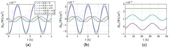
Figure 3. The geomagnetic field intensity on a circular orbit with an orbital height of 500 km: (a) $B_{\mathrm{E}x}$; (b) $B_{\mathrm{E}y}$; (c) $B_{\mathrm{E}z}$.

The disturbance torque acting on the satellite due to the earth’s magnetic field [8] can be written as

$${\mathit{\tau }}_{\mathrm{E}}={\mathit{\mu }}^{\mathrm{CM}}\times {\mathit{B}}_{\mathrm{E}}^{\mathrm{CM}}=\left[\begin{array}{c}{\mu }_y{B}_{\mathrm{E}z}-{\mu }_z{B}_{\mathrm{E}y}\\ {\mu }_z{B}_{\mathrm{E}x}-{\mu }_x{B}_{\mathrm{E}z}\\ {\mu }_x{B}_{\mathrm{E}y}-{\mu }_y{B}_{\mathrm{E}x}\end{array}\right]$$

(19)

Since the z component of the geomagnetic field expressed in the orbital coordinate frame has a constant part, the angular momentum on the satellites will inevitably accumulate if no effective measures are taken for the magnetic dipoles.

3. Magnetic Dipole Assignment

The current of the electromagnetic coils has a maximum limit, so it is necessary to consider the problem of control input saturation of electromagnetic formation. The maximum inter-satellite electromagnetic force provided by the magnetic dipoles depends on the inter-satellite distance, the maximum current of the coils, and the direction of the magnetic dipoles. This section analyzes the electromagnetic force envelope, dipole assignment, and optimization of the two-satellite electromagnetic formation.

3.1. Electromagnetic Force Envelope

The electromagnetic force envelope is the electromagnetic force range the system can provide in all directions when the maximum current enters the electromagnetic coils. Let $g\left(\gamma \right)=‖\mathit{F}‖/A_0$, $g\left(\gamma \right)$ reflect the control ability of electromagnetic formation. The range in $g\left(\gamma \right)$ is the envelope of the gray area in Figure 4. This envelope [31] shows the relationship between the electromagnetic force and the magnetic dipole, providing a theoretical analysis basis for dipole assignment.

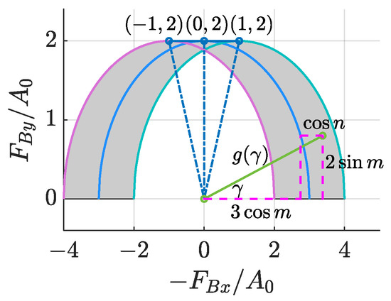
Figure 4. The electromagnetic force envelope.

3.2. Magnetic Dipole Assignment

EMFF must provide the required control force for each satellite in the formation in real time. It is crucial to assign the magnetic dipoles for each satellite reasonably. Because the system has a certain degree of freedom, the magnetic dipoles have infinite solutions so that we can set the optimization objectives according to the task requirements.

This paper discusses the analytical solutions of magnetic dipoles with energy optimization and differentiability, respectively, according to the electromagnetic force envelope.

(1) Optimal energy strategy

The optimal energy strategy refers to the magnetic dipole assignment strategy to achieve the minimum power consumption of electromagnetic coils for a specific electromagnetic force. Since the electric power consumption of the coil is proportional to the square of the current, and the magnetic dipole is proportional to the current, the objective function of the optimal energy strategy can be expressed as $J=\min \left({\mu }_A^2+{\mu }_B^2\right)=\min \left(\frac{16\pi d^4{A}_0}{3{\mu }_0}\right)$. Thus, $J$ is proportional to $A_0$. The maximum envelope of electromagnetic force refers to the maximum electromagnetic force that the system can provide in all directions when passing the maximum current through the electromagnetic coils. When the maximum electromagnetic force envelope is selected for a specific electromagnetic force, $A_0$ is the minimum, and $J$ is the minimum.

The magnetic dipole solution with the minimum energy consumption of the electromagnetic coils [31] corresponds to the envelope of the maximum electromagnetic force. When $0\le \gamma <\arctan 2$ holds, then $\cos n=1$; when $\pi -\arctan 2<\gamma \le \pi$ holds, then $\cos n=-1$; when $\arctan 2\le \gamma \le \pi -\arctan 2$ holds, then $\sin m=1$. $m,n$ are piecewise functions varying with $\gamma$, and they are continuous but nondifferentiable at the piecewise point. When $\gamma$ varies in multiple intervals, the magnetic dipole solution with the minimum energy consumption is continuous but nondifferentiable at the segmentation point, so the disturbance torque acting on the satellite from the earth’s magnetic field is nondifferentiable.

(2) Magnetic dipole solution differentiable strategy

We propose another magnetic dipole assignment strategy to ensure the magnetic dipole solution’s differentiability and optimize energy consumption. The smooth electromagnetic force envelope can ensure the differentiability of dipole solution at any moment of EMFF. In addition, the larger the electromagnetic force envelope, the smaller the energy consumption of the coils. The elliptical electromagnetic force envelope passing through points $\left(4,0\right)$ and $\left(0,2\right)$ satisfies the above requirements. At this time, the parameters have the following relationship.

$$\beta =0,\begin{array}{c}\end{array}g\cos \gamma =4\cos \alpha ,\begin{array}{c}\end{array}g\sin \gamma =2\sin \alpha ,\begin{array}{c}\end{array}g=2\sqrt{1+3{\cos }^2\alpha }$$

(20)

The maximum electromagnetic force envelope and the maximum elliptical electromagnetic force envelope of $g\left(\gamma \right)=‖\mathit{F}‖/A_0$ are shown in Figure 5a. The corresponding curves of $\left(\alpha ,\beta \right)$ and $g\left(\gamma \right)$ changing with $\gamma$ are shown in Figure 5b,c. $\left({\alpha }_1,{\beta }_1\right)$ corresponds to the maximum envelope of $g\left(\gamma \right)$, and $\left({\alpha }_2,{\beta }_2\right)$ corresponds to the maximum ellipse envelope of $g\left(\gamma \right)$.

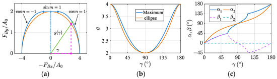
Figure 5. Maximum envelope and maximum ellipse envelope: (a) Envelopes; (b) $g\left(\gamma \right)$; (c) $\alpha ,\beta$.

The optimal energy strategy minimizes coil energy consumption. The magnetic dipole differentiable strategy can ensure that the disturbance torque from the geomagnetic field on the electromagnetic satellite is continuously differentiable, which is conducive to further improving the attitude control accuracy.

3.3. Angular Momentum Management

Due to the disturbance torque from the geomagnetic field, the angular momentum of the reaction wheel increases rapidly when the reaction wheel is used to control the satellites’ attitude. Therefore, taking some measures to manage the angular momentum of the reaction wheel is crucial. The polarity reversal and the frequency division methods for angular momentum management are discussed below.

(1) Polarity reversal method

The polarity reversal operation changes the magnetic dipoles’ signs at regular intervals. According to Equation (5), the inter-satellite electromagnetic force does not vary. According to Equation (19), the disturbance torque from the geomagnetic field act on the satellite changes sign. When the polarity reversal period is short, resulting in a net cancellation of the effect of the geomagnetic field on average.

(2) Frequency division method

The magnetic dipole of each satellite is excited by a fixed sinusoidal current source whose frequency is much higher than the formation orbit frequency.

The magnetic dipoles in the electromagnetic frame can be expressed as

$$\left\{\begin{array}{l}{\mathit{\mu }}_A=\cos \left({\omega }_{f}t\right){\mu }_A{\left[\cos \alpha \hspace{1em}\sin \alpha \hspace{1em}0\right]}^{\mathrm{T}}\\ {\mathit{\mu }}_B=\cos \left({\omega }_{f}t\right){\mu }_B{\left[\cos \beta \hspace{1em}\sin \beta \hspace{1em}0\right]}^{\mathrm{T}}\end{array}\right.$$

(21)

where ${\omega }_f$ is the carrier frequency. It can be seen from Equation (21) that the frequency division strategy can ensure the continuity of the magnetic dipole solution.

At this time, the electromagnetic force/torque is expressed as

$$\left\{\begin{array}{l}{\mathit{F}}^{\mathrm{EM}}=\frac{1+\cos \left(2{\omega }_{f}t\right)}{2}{A}_0{\left[-\left(3\cos m+\cos n\right)\hspace{1em}2\sin m\hspace{1em}0\right]}^{\mathrm{T}}\\ {\mathit{\tau }}_A=\frac{1+\cos \left(2{\omega }_{f}t\right)}{2}{A}_1{\left[0\hspace{1em}0\hspace{1em}3\sin m+\sin n\right]}^{\mathrm{T}}\\ {\mathit{\tau }}_B=\frac{1+\cos \left(2{\omega }_{f}t\right)}{2}{A}_1{\left[0\hspace{1em}0\hspace{1em}3\sin m-\sin n\right]}^{\mathrm{T}}\end{array}\right.$$

(22)

From the above formula, it can be seen that both electromagnetic force and electromagnetic torque contain constant and harmonic components. The constant part of the electromagnetic force is used for the control input of effective relative position control. In contrast, the harmonic part forms a disturbance force and must be eliminated or compensated. The effective electromagnetic force is 1/2 of that without the frequency division.

For the electromagnetic formation in low Earth orbit, the magnetic dipoles show periodicity using the frequency division method, and the modulation period is far less than the orbital period. According to Equation (19), the disturbance torque from the geomagnetic field acting on the satellites will show a periodicity with an average value of almost zero.

4. Electromagnetic Formation Flight Control

Given the highly nonlinear and coupling characteristics of the dynamics of the electromagnetic formation, we propose centralized control for translational motion and decentralized control for attitude motion by regarding the electromagnetic torque between satellites as interference torque. The electromagnetic model used in this paper is the far-field model, and its model error can reach about 10% when the satellites are very close. In addition, the inertia matrix of the satellite also has some uncertainty. Active disturbance rejection control (ADRC) provides a control method for online estimation and compensation of the total uncertainty. Because the total uncertainty is compensated in time, the expected transient performance of the closed-loop system can be achieved [32,33,34,35]. Considering these factors, we propose a control scheme using ADRC to compensate for the system’s unmodeled dynamics and external disturbance estimates. The control purpose of this paper is to ensure the translational and attitude control accuracy of formation satellites, keep the angular momentum of reaction wheels within the allowable range, and avoid rapid accumulation as much as possible. The control diagram is shown in Figure 6.

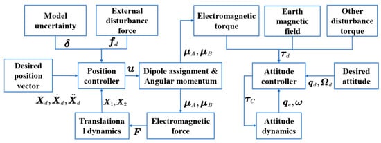
Figure 6. The control diagram.

4.1. Translation Control

Equation (9) gives the translational dynamic equation of the two-satellite electromagnetic formation. Assuming the expected state of the relative position of the two satellites is ${\mathit{X}}_d={\left[\begin{array}{ccc}{x}_d& y_d& z_d\end{array}\right]}^{\mathrm{T}},{\dot{\mathit{X}}}_d={\left[\begin{array}{ccc}{\dot{x}}_d& {\dot{y}}_d& {\dot{z}}_d\end{array}\right]}^{\mathrm{T}}$, let ${\mathit{X}}_1={\left[\begin{array}{ccc}x-x_d& y-y_d& z-z_d\end{array}\right]}^{\mathrm{T}}$, ${\mathit{X}}_2={\left[\begin{array}{ccc}\dot{x}-{\dot{x}}_d& \dot{y}-{\dot{y}}_d& \dot{z}-{\dot{z}}_d\end{array}\right]}^{\mathrm{T}}$. The electromagnetic model in this paper adopts the far-field electromagnetic model. The accurate electromagnetic model is usually considered as the sum of the far-field model term and the correction term [8]. $\mathit{\delta }=diag\left({\delta }_x,{\delta }_y,{\delta }_z\right)$ is the unknown gain parameter obtained through measurement, and $\mathit{\delta }\cdot \mathit{u}={\left[\begin{array}{ccc}{\delta }_x{u}_x& {\delta }_y{u}_y& {\delta }_z{u}_z\end{array}\right]}^{\mathrm{T}}$ is the correction term. System (9) can be rewritten as

$$\left\{\begin{array}{l}{\dot{\mathit{X}}}_1={\mathit{X}}_2\\ {\dot{\mathit{X}}}_2=\mathit{u}+\mathit{f}\end{array}\right.$$

(23)

where $\mathit{f}={\mathit{A}}_1{\mathit{X}}_1+{\mathit{A}}_2{\mathit{X}}_2+{\mathit{A}}_1{\mathit{X}}_d+{\mathit{A}}_2{\dot{\mathit{X}}}_d-{\ddot{\mathit{X}}}_d+\mathit{\delta }\mathit{u}+{\mathit{f}}_d$, ${\mathit{A}}_1=\left[\begin{array}{ccc}3{\omega }_0^2& 0& 0\\ 0& 0& 0\\ 0& 0& -{\omega }_0^2\end{array}\right],{\mathit{A}}_2=\left[\begin{array}{ccc}0& 2{\omega }_0& 0\\ -2{\omega }_0& 0& 0\\ 0& 0& 0\end{array}\right]$.

According to [34], the following linear extended state observer (LESO) is designed for system (23).

$$\left\{\begin{array}{l}{\dot{\hat{\mathit{X}}}}_1={\hat{\mathit{X}}}_2-{\mathit{\beta }}_1\left({\hat{\mathit{X}}}_1-{\mathit{X}}_1\right)\\ {\dot{\hat{\mathit{X}}}}_2=\mathit{u}+\hat{\mathit{f}}-{\mathit{\beta }}_2\left({\hat{\mathit{X}}}_1-{\mathit{X}}_1\right)\\ \dot{\hat{\mathit{f}}}=-{\mathit{\beta }}_3\left({\hat{\mathit{X}}}_1-{\mathit{X}}_1\right)\end{array}\right.$$

(24)

where ${\mathit{\beta }}_k=diag\left({\beta }_{k1},{\beta }_{k2},{\beta }_{k3}\right),k=1,2,3$.

The characteristic equation of observer (24) is summarized as

$$\lambda \left(s\right)=\left(s^3+{\beta }_{11}{s}^2+{\beta }_{21}s+{\beta }_{31}\right)\left(s^3+{\beta }_{12}{s}^2+{\beta }_{22}s+{\beta }_{32}\right)\left(s^3+{\beta }_{13}{s}^2+{\beta }_{23}s+{\beta }_{33}\right)$$

(25)

The observer gain parameters are designed to satisfy that $L_{tj}=s^3+{\beta }_{1j}{s}^2+{\beta }_{2j}s+{\beta }_{3j},j=1,2,3$ are Hurwitz polynomials. According to [34], let ${\beta }_{1j}=3{\omega }_{otj},{\beta }_{2j}=3{\omega }_{otj}^2,{\beta }_{3j}={\omega }_{otj}^3,{\omega }_{otj}>0,j=1,2,3$, then $L_{tj}={\left(s+{\omega }_{otj}\right)}^3$. LESO has estimated the impact of both model dynamics (including unmodeled dynamics and uncertainties) and external disturbances.

If ${\mathit{X}}_1$ and ${\mathit{X}}_2$ are measurable and reliable, estimating them is unnecessary, and the reduced-order ESO can be designed as

$$\dot{\hat{\mathit{f}}}=-{\mathit{\beta }}_4\left(\hat{\mathit{f}}-\mathit{f}\right)=-{\mathit{\beta }}_4\left(\hat{\mathit{f}}-{\dot{\mathit{X}}}_2+\mathit{u}\right)$$

(26)

where ${\mathit{\beta }}_4=diag\left({\beta }_{41},{\beta }_{42},{\beta }_{43}\right),{\beta }_{4j}={\omega }_{otj},{\omega }_{otj}>0,j=1,2,3$.

Equation (26) can be rewritten as

$$\left\{\begin{array}{l}\dot{\xi }=-{\mathit{\beta }}_4\left(\mathit{u}+{\mathit{\beta }}_4{\mathit{X}}_2+\xi \right)\\ \hat{\mathit{f}}={\mathit{\beta }}_4{\mathit{X}}_2+\xi \end{array}\right.$$

(27)

where $\mathit{\xi }\left(t_0\right)=-{\mathit{\beta }}_4{\mathit{X}}_2\left(t_0\right)$.

Based on the online estimation of total disturbance, ADRC can be designed as

$$\mathit{u}=-{\mathit{k}}_1{\mathit{X}}_1-{\mathit{k}}_2{\mathit{X}}_2-\hat{\mathit{f}}$$

(28)

where ${\mathit{k}}_1={\mathit{\omega }}_{ct}^2$ and ${\mathit{k}}_2=2{\mathit{\omega }}_{ct}$ can be set for simplicity, and ${\mathit{\omega }}_{ct}=diag\left({\omega }_{ct1},{\omega }_{ct2},{\omega }_{ct3}\right),{\omega }_{ctj}>0,j=1,2,3$ is the controller bandwidth. References [34,35] analyzed the convergence of linear ADRC for such MIMO systems and proved that the error between the closed-loop system trajectory based on ADRC and the reference closed-loop system trajectory is limited by a bound.

The maximum current value constrains the electromagnetic force between satellites, and the maximum control input that the system can provide is expressed as

$$u_{\max }=\frac{3{\mu }_0}{8\pi }\frac{{\mu }_A\cdot {\mu }_B}{d^4}\frac{m_A+m_B}{m_A{m}_B}\cdot g\left(\gamma \right)$$

(29)

To treat the control constraints, we rewrite the control input as

$$\mathit{u}=sat\left(u_{\max }/‖\mathit{u}‖\right)\mathit{u}$$

(30)

where $sat\left(u_{\max }/‖\mathit{u}‖\right)=\min \{1,u_{\max }/‖\mathit{u}‖\}$.

4.2. Attitude Control

The following mild assumptions for the systems (12)–(16) are given:

(1) Each satellite in the formation is equipped with three orthogonal reaction wheels for decentralized control of satellite attitude.

(2) In the satellite attitude model Equation (12), full states can be measured. This implies that the unit-quaternion $\mathit{q}$ and the angular velocity $\mathbf{\Omega }$ are available in the controller design.

(3) The satellite’s inertial matrix is $\mathit{J}={\mathit{J}}_0+\Delta \mathit{J}$, where ${\mathit{J}}_0$ selected nonsingular is the known constant matrix. $\Delta \mathit{J}$ is the uncertainty part of the inertial matrix.

Because of $\left({\mathit{J}}_0{}^{-1}-{\mathit{J}}_0{}^{-1}\Delta \mathit{J}{\left({\mathit{J}}_0+\Delta \mathit{J}\right)}^{-1}\right)\left({\mathit{J}}_0+\Delta \mathit{J}\right)={\mathit{I}}_{3\times 3}$, we can obtain ${\mathit{J}}^{-1}={\mathit{J}}_0{}^{-1}-{\mathit{J}}_0{}^{-1}\Delta \mathit{J}{\mathit{J}}^{-1}$. Equation (16) can be summarized as

$$\begin{array}{l}{\dot{\mathit{q}}}_e=\frac{1}{2}M\left({\mathit{q}}_e\right)\mathit{\omega }=\frac{1}{2}\left[\begin{array}{c}-{\mathit{q}}_{ev}^{\mathrm{T}}\\ \left(q_{e0}{\mathit{I}}_3+{\mathit{q}}_{ev}^{\times }\right)\end{array}\right]\mathit{\omega }\\ \dot{\mathit{\omega }}=-{\mathit{J}}^{-1}{\left(\mathit{\omega }+\mathit{C}{\mathbf{\Omega }}_d\right)}^{\times }\mathit{J}\left(\mathit{\omega }+\mathit{C}{\mathbf{\Omega }}_d\right)+\left({\mathit{\omega }}^{\times }\mathit{C}{\mathbf{\Omega }}_d-\mathit{C}{\dot{\mathbf{\Omega }}}_d\right)-\Delta \mathit{J}\dot{\mathit{\omega }}+{\mathit{J}}_0{}^{-1}{\mathit{\tau }}_c-{\mathit{J}}_0{}^{-1}\Delta \mathit{J}{\mathit{J}}^{-1}{\mathit{\tau }}_c+{\mathit{J}}^{-1}{\mathit{\tau }}_d\\ ={\mathit{J}}_0{}^{-1}{\mathit{\tau }}_c+\Delta \end{array}$$

(31)

where $\Delta$ represents the total uncertainty of the system, expressed as $\Delta =-{\mathit{J}}_0{}^{-1}\Delta \mathit{J}{\mathit{J}}^{-1}{\mathit{\tau }}_c-{\mathit{J}}^{-1}{\left(\mathit{\omega }+\mathit{C}{\mathbf{\Omega }}_d\right)}^{\times }\mathit{J}\left(\mathit{\omega }+\mathit{C}{\mathbf{\Omega }}_d\right)+{\mathit{\omega }}^{\times }\mathit{C}{\mathbf{\Omega }}_d-\mathit{C}{\dot{\mathbf{\Omega }}}_d+{\mathit{J}}^{-1}{\mathit{\tau }}_d$.

In this paper, we aim to design a feedback controller so that the state of the closed-loop system (12) tracks the desired attitude motion (14), which can be expressed as follows.

$$\underset{t\to \infty }{\lim }{\mathit{q}}_e(t)={\left[\begin{array}{cccc}1& 0& 0& 0\end{array}\right]}^{\mathrm{T}},\begin{array}{c}\end{array}\underset{t\to \infty }{\lim }\mathit{\omega }(t)=0$$

(32)

According to Equation (11), the control objective can be expressed as

$$\underset{t\to \infty }{\lim }\mathit{\theta }(t)=0,\begin{array}{c}\end{array}\underset{t\to \infty }{\lim }\mathit{\omega }(t)=0$$

(33)

Then to estimate the unknown uncertainties $\Delta$, the following linear extended state observer (LESO) can be designed.

$$\left\{\begin{array}{l}\dot{\hat{\mathit{\omega }}}={\mathit{J}}_0^{-1}{\mathit{\tau }}_c+\hat{\Delta }-{\mathit{\gamma }}_1\left(\hat{\mathit{\omega }}-\mathit{\omega }\right)\\ \dot{\hat{\Delta }}=-{\mathit{\gamma }}_2\left(\hat{\mathit{\omega }}-\mathit{\omega }\right)\end{array}\right.$$

(34)

The observer gain is ${\mathit{\gamma }}_k=diag\left({\gamma }_{k1},{\gamma }_{k2},{\gamma }_{k3}\right),k=1,2$. The design gain parameters satisfy the condition that $L_{aj}=s^2+{\gamma }_{1j}s+{\gamma }_{2j},j=1,2,3$ are Hurwitz polynomials. Let ${\gamma }_{1j}=2{\omega }_{oaj},{\gamma }_{2j}={\omega }_{oaj}^2,{\omega }_{oaj}>0,j=1,2,3$, then $L_{aj}={\left(s+{\omega }_{oaj}\right)}^2$. The outputs $\hat{\mathit{\omega }}$ and $\hat{\Delta }$ of ESO (34) are used to estimate $\mathit{\omega }$ and $\Delta$, respectively. Refs. [34,35] proved that the estimation error could be as small as possible.

If $\mathit{\omega }$ is measurable and reliable, estimating it is unnecessary, and the reduced-order ESO can be designed as

$$\dot{\hat{\Delta }}=-{\mathit{\gamma }}_3\left(\hat{\Delta }-\Delta \right)=-{\mathit{\gamma }}_3\left(\hat{\Delta }-\dot{\mathit{\omega }}+{\mathit{J}}_0^{-1}{\mathit{\tau }}_c\right)$$

(35)

where ${\mathit{\gamma }}_3=diag\left({\gamma }_{31},{\gamma }_{32},{\gamma }_{33}\right),{\gamma }_{3j}={\omega }_{oaj},j=1,2,3$

It can be further reorganized as

$$\left\{\begin{array}{l}{\dot{\mathit{\xi }}}_2=-{\mathit{\gamma }}_3\left({\mathit{J}}_0{}^{-1}{\mathit{\tau }}_c+{\mathit{\gamma }}_3\mathit{\omega }+{\mathit{\xi }}_2\right)\\ \hat{\Delta }={\mathit{\gamma }}_3\mathit{\omega }+{\mathit{\xi }}_2\end{array}\right.$$

(36)

where ${\mathit{\xi }}_2\left(t_0\right)=-{\mathit{\gamma }}_3\mathit{\omega }\left(t_0\right)$.

Then based on the online estimation of total disturbance or extended state, the controller is designed as

$$\left\{\begin{array}{l}\overline{\mathit{\omega }}=-{\mathit{k}}_3\mathit{\theta }\\ {\mathit{\tau }}_c={\mathit{J}}_0\left(-\left({\mathit{k}}_3+{\mathit{k}}_4\right)\mathit{\omega }-{\mathit{k}}_3{\mathit{k}}_4\mathit{\theta }-\hat{\Delta }\right)\end{array}\right.$$

(37)

where $\overline{\mathit{\omega }}$ is the virtual control. For simplicity, we can set ${\mathit{k}}_3=\frac{1}{2}{\mathit{\omega }}_{ca},{\mathit{k}}_4=2{\mathit{\omega }}_{ca}$, where ${\mathit{\omega }}_{ca}=diag\left({\omega }_{ca1},{\omega }_{ca2},{\omega }_{ca3}\right),{\omega }_{caj}>0,j=1,2,3$ is the controller bandwidth. The controller bandwidth is adjusted according to the tracking convergence speed and stability. A larger controller bandwidth will improve the response speed but make the system more noise-sensitive, leading to system oscillation.

From Equations (31) and (37), we get the reference error system:

$$\left\{\begin{array}{l}{\dot{\overline{\mathit{e}}}}_1=\dot{\mathit{\theta }}=\mathit{\omega }={\overline{\mathit{e}}}_2+\overline{\mathit{\omega }}={\overline{\mathit{e}}}_2-{\mathit{k}}_3{\overline{\mathit{e}}}_1\\ {\dot{\overline{\mathit{e}}}}_2=\dot{\mathit{\omega }}-\dot{\overline{\mathit{\omega }}}={\mathit{J}}_0{}^{-1}{\mathit{\tau }}_c+\Delta +{\mathit{k}}_3\mathit{\omega }=-{\mathit{k}}_4{\overline{\mathit{e}}}_2-\hat{\Delta }+\Delta \end{array}\right.$$

(38)

where ${\overline{\mathit{e}}}_1=\mathit{\theta }$,${\overline{\mathit{e}}}_2=\mathit{\omega }-\overline{\mathit{\omega }}$.

Lemma 1

(Lohmiller. W. et al. [36]). A system with a virtual dynamics of the form

$$\frac{d}{dt}\left(\begin{array}{l}\delta z_1\hfill \\ \delta z_2\hfill \end{array}\right)=\left(\begin{array}{cc}{F}_{11}& 0\\ F_{21}& F_{22}\end{array}\right)\left(\begin{array}{l}\delta z_1\hfill \\ \delta z_2\hfill \end{array}\right)$$

(39)

is known as the hierarchical combination. The system will be converging if the submatrices $F_{11}$ and $F_{22}$ are uniformly negative definite and $F_{21}$ is bounded. furthermore, with Bounded disturbance ${\Theta }_1{d}_1$ added to the $\delta z_1$ dynamics and Bounded disturbance ${\Theta }_2{d}_2$ added to the $\delta z_2$ dynamics, the system exponential convergence to a ball around the desired trajectory.

We note that the error system (38) is a hierarchical combination system, and $\left(-\hat{\Delta }+\Delta \right)$ can be considered a bounded disturbance added to ${\overline{\mathit{e}}}_2$ dynamics. According to Lemma 1, the error system can converge exponentially to a ball around the origin.

5. Simulation Analysis

In this section, a two-satellite electromagnetic formation flight near-Earth orbit is simulated and used to verify the effectiveness of the control method and the angular momentum management strategies. Suppose that the formation center of mass is running in a circular orbit at an altitude of 500 km, and the attitude of the satellites is consistent with the orbital frame. The two satellites maintain a fixed distance $d=20\hspace{1em}\mathrm{m}$, the relative motion period of the satellites is $T=5\hspace{1em}\mathrm{h}$, and the relative position vector of the satellites is designed as ${\mathit{\rho }}^{\mathrm{CM}}=\frac{d}{2}{\left[\begin{array}{ccc}\sin \left(\omega t\right)& \sqrt{3}\sin \left(\omega t\right)& 2\cos \left(\omega t\right)\end{array}\right]}^{\mathrm{T}}$, where $\omega =2\pi /T$. The mass of each satellite is 150 kg, and the inertia matrix is $\mathit{J}=diag\left(20,17,24\right)\mathrm{kg}\cdot {\mathrm{m}}^2$; the maximum magnetic dipoles are ${\mu }_{\max }={10}^5\mathrm{A}\cdot {\mathrm{m}}^2$; the maximum output torque of the reaction wheels is ${\tau }_{\max }=2\mathrm{N}\cdot \mathrm{m}$. The initial relative position is ${\left[\begin{array}{ccc}-1& -2& 17\end{array}\right]}^{\mathrm{T}}\mathrm{m}$, and the initial relative angular velocity vector is ${\left[\begin{array}{ccc}0.0326& -0.0055& -0.0200\end{array}\right]}^{\mathrm{T}}\mathrm{m}/\mathrm{s}$.

Assume that the inertial uncertainty of the satellite is $\Delta \mathit{J}=diag\left(1,-2,3\right)$ and the uncertainty of the electromagnetic far-field model is 8%. In the simulation design, the initial deviation and the external disturbance force and torque mainly caused by the J2 perturbation of the earth and the effect of the earth’s magnetic field are added to each channel. The external disturbance force ${\mathit{f}}_d={10}^{-5}\times {\left[\begin{array}{ccc}6\sin \left({\omega }_{0}t+\pi /6\right)& -5\times \sin \left({\omega }_{0}t+\pi /3\right)& -4\sin {\omega }_{0}t\end{array}\right]}^{\mathrm{T}}\mathrm{m}/{\mathrm{s}}^2$ is assumed to be a sinusoidal noise varying with the orbital period. The disturbance torque on the satellites mainly comes from the earth’s magnetic field. The inter-satellite electromagnetic torque and the disturbance torque on the satellites from the earth’s magnetic field are solved by Equations (4) and (16), respectively. In addition, assuming the electromagnetic satellite is also subject to other periodic external disturbance torque of ${\mathit{\tau }}_d={\left[\begin{array}{ccc}0.01\sin \left({\omega }_{0}t\right)& -0.01\sin \left({\omega }_{0}t\right)& 0.02\cos \left({\omega }_{0}t\right)\end{array}\right]}^{\mathrm{T}}\mathrm{N}\cdot \mathrm{m}$. The initial state errors of the relative translational motion are chosen as ${\mathit{X}}_1\left(0\right)={\left[\begin{array}{ccc}-1& -2& 2\end{array}\right]}^{\mathrm{T}}\mathrm{m}$ and ${\mathit{X}}_2\left(0\right)={\left[\begin{array}{ccc}0.03& -0.01& -0.02\end{array}\right]}^{\mathrm{T}}\mathrm{m}/\mathrm{s}$. The initial error quaternion of satellite A is ${\mathit{e}}_A\left(0\right)={\left[\begin{array}{cccc}0.2& -0.2& 0.3& 0.767\end{array}\right]}^{\mathrm{T}}$, and the initial angular velocity error is ${\mathit{\omega }}_A\left(0\right)={\left[\begin{array}{ccc}-0.3& -0.1& 0.5\end{array}\right]}^{\mathrm{T}}\mathrm{rad}/\mathrm{s}$. The dynamics of the electromagnetic formation system are simulated using the numerical differential equation solver ODE45 in a personal notebook.

5.1. Optimal Energy Strategy

The control parameters for numerical simulation are designed as ${\omega }_{otj}=0.06,{\omega }_{ctj}=0.06,{\omega }_{oaj}=1,{\omega }_{caj}=0.3,j=1,2,3$. Figure 7 gives the three-dimensional configuration of the formation, the relative position error, the relative velocity error, and the inter-satellite electromagnetic force acceleration. The relative position and relative velocity errors converge to a small boundary containing 0 within 150 s, and the steady-state errors are less than $3.7\times {10}^{-4}$ m and $3.5\times {10}^{-7}$ m/s in the presence of model uncertainty and external disturbance. The system has achieved high control accuracy and can meet the requirements of many engineering applications, implying the proposed controller can estimate and compensate for the total disturbance of the system well.

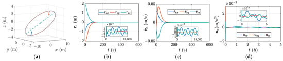
Figure 7. Tracking errors of the relative translational states and control input: (a) Relative motion trajectory; (b) Relative position error; (c) Relative velocity error; (d) Electromagnetic force acceleration.

The magnetic dipole assignment with the energy optimization strategy is shown in Figure 8a. The magnetic dipole solution curve is continuous, and there are cusps at some points, that is, nondifferentiable points determined by the characteristics of the maximum envelope of the electromagnetic force. Figure 8b displays the curves of disturbance torque acting on satellite A from the geomagnetic field, and the curves are also continuous and nondifferentiable at the cusps. Take satellite A as an example. Figure 8c–f displays the attitude error, angular velocity error, the control torque input, and the angular momentum of the reaction wheels varying with time. The attitude and angular velocity errors converge to the small boundary within 40 s, and the steady-state errors are less than $1.2\times {10}^{-3}$ and $5\times {10}^{-4}$ rad/s, respectively. There are significant convergence errors at the non-differentiable points.

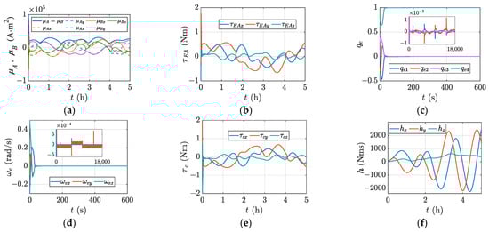
Figure 8. Magnetic dipole assignment and attitude tracking control with the energy optimization strategy: (a) Magnetic dipoles; (b) Disturbance torque from the geomagnetic field. (c) Attitude error; (d) Angular velocity error; (e) Control torque input; (f) Angular momentum of the reaction wheels.

5.2. Dipole Solution Differentiable Strategy

The magnetic dipole assignment with the solution differentiable strategy and the differentiable disturbance torque acting on satellite A from the geomagnetic field are illustrated in Figure 9a,b. The resulting curves of satellite A in attitude error, angular velocity error, control torque, and angular momentum are presented in Figure 9c–f. Compared with the control under the energy optimization strategy, the attitude control accuracy is improved, but the angular momentum accumulation is slightly increased. The differentiable magnetic dipole solution is conducive to enhancing attitude control accuracy.

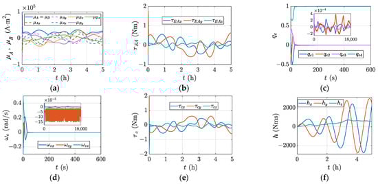
Figure 9. Magnetic dipole assignment and attitude tracking control with the solution differentiable strategy: (a) Magnetic dipoles; (b) Disturbance torque from the geomagnetic field; (c) Attitude error; (d) Angular velocity error; (e) Control torque input; (f) Angular momentum of the reaction wheels.

5.3. Polarity Reversal Strategy

The magnetic dipoles of the two satellites with the energy optimization strategy switch their pole signs every 100 s. Figure 10a,b gives the magnetic dipole assignment with the polarity reversal strategy. The magnetic dipoles are discontinuous at the switching points, causing the disturbance torque on satellites from the geomagnetic field to be discontinuous at the switching points. The curves of satellite A in attitude error, angular velocity error, control torque, and angular momentum are depicted in Figure 10c–f. Because the disturbance torque from the geomagnetic field is discontinuous when the magnetic poles are switched, the attitude and angular velocity tracking error of the satellite becomes larger. The attitude control accuracy of this strategy is one order of magnitude lower than the control accuracy without switching. However, the polarity reversal method can dramatically reduce angular momentum accumulation.

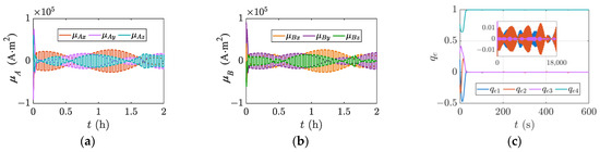
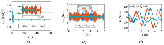
Figure 10. Magnetic dipoles’ solution and attitude tracking control under pole reversal (switching every 100 s) strategy: (a) Dipole A; (b) Dipole B; (c) Attitude error; (d) Angular velocity error; (e) Control torque input; (f) Angular momentum of the reaction wheels.

Figure 11a,b gives the magnetic dipole assignment with the energy optimization strategy and the polarity reversal strategy, and the dipoles shift polarity every 20 s. The curves of satellite A in attitude error, angular velocity error, control torque, and angular momentum are depicted in Figure 11c–f. Compared with the switching period of 100 s, the frequency of pole switching increases so that the accumulation of angular momentum of the reaction wheel is in a smaller range over a period.

Figure 11. Magnetic dipoles’ solution and attitude tracking control under pole reversal (switching every 20 s) strategy: (a) Dipole A; (b) Dipole B; (c) Attitude error; (d) Angular velocity error; (e) Control torque input; (f) Angular momentum of the reaction wheels.

5.4. Frequency Division Strategy

The magnetic dipoles are modulated with carrier current, where the carrier frequency is set as ${\omega }_f=0.1\pi$. Control parameters are set as ${\omega }_{otj}=0.06,{\omega }_{ctj}=0.03,{\omega }_{oaj}=4,{\omega }_{caj}=0.7,j=1,2,3$. Figure 12 gives the relative translational states tracking errors and magnetic dipole assignment, where the magnetic dipole solution shown in Figure 12d are the magnetic dipoles not multiplied by the carrier current. The relative position and relative velocity errors converge to a small boundary containing 0 within 210 s, which shows that the ADRC scheme can well estimate and compensate for the harmonic disturbance generated by the frequency division strategy.

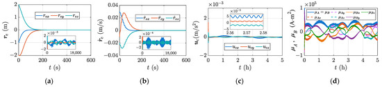
Figure 12. Tracking errors of the relative translational states and control input: (a) Relative position error; (b) Relative velocity error; (c) Electromagnetic force acceleration; (d) Magnetic dipoles.

As shown in Figure 13a,b, the tracking errors of attitude and angular velocity of satellite A can converge quickly, and the control accuracy is an order of magnitude higher than the polarity reversal strategy. The control torque in Figure 13c changes periodically with the carrier current, and the angular momentum in Figure 13d of satellite A is in a small range for a long time.

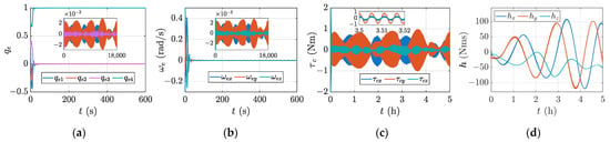
Figure 13. Attitude tracking error and control torque input under frequency division strategy: (a) Attitude error; (b) Angular velocity error; (c) Control torque input; (d) Angular momentum of the reaction wheels.

Table 1 compares simulation results of relative translational and attitude motion under different magnetic dipole assignment strategies and angular momentum management strategies. The results show that the differentiability of the magnetic dipole is conducive to reducing the steady-state error of the electromagnetic satellite’s attitude, thus improving the control performance of the formation. The magnetic pole switching strategy generates a larger steady-state error of the satellite’s attitude because the magnetic pole switching makes the disturbance torque from the geomagnetic field on the electromagnetic satellite discontinuous, thus affecting the LESO’s ability to estimate the external disturbance. The magnetic pole switching strategy and frequency division method can ensure that the angular momentum of the satellite is maintained in a small range for a long period, significantly improving the rapid accumulation of the angular momentum of the reaction wheel. In addition, the frequency of magnetic pole switching also affects the satellite attitude’s steady-state error and angular momentum accumulation. More frequent switching keeps the angular momentum in a small range. The frequency division method not only produces effective electromagnetic control force but also brings interference force varying with the magnetic dipole, which impacts the steady state error of the relative position of the satellite. Compared with the magnetic pole switching strategy, the control accuracy of the satellite’s relative position is reduced, while the control accuracy of the attitude is improved.

Table 1. Simulation results of different magnetic dipole allocation and angular momentum management strategies.

Strategies	Relative Position Error (m)	Relative Velocity Error (m/s)	Quaternion Error	Angular Velocity Error (rad/s)	Angular Momentum Range (Nms)
Energy optimization	$3.7\times {10}^{-4}$	$3.5\times {10}^{-7}$	$1.2\times {10}^{-3}$	$5\times {10}^{-4}$	$-2257\sim 2455$
Differentiable dipole solution			$4\times {10}^{-4}$	$1.5\times {10}^{-5}$	$-2759\sim 2998$
Polarity reversal (switching every 100 s) + energy optimization			$1.2\times {10}^{-2}$	$2.4\times {10}^{-2}$	$-207\sim 187$
Polarity reversal (switching every 20 s) + energy optimization			$1.5\times {10}^{-2}$	$3.0\times {10}^{-2}$	$-87\sim 74$
Frequency division + energy optimization	$1.8\times {10}^{-3}$	$2.1\times {10}^{-4}$	$2.8\times {10}^{-3}$	$2.9\times {10}^{-3}$	$-117\sim 106$
Frequency division + differentiable dipole solution	$2.3\times {10}^{-3}$	$2.0\times {10}^{-4}$	$2.2\times {10}^{-3}$	$2.4\times {10}^{-3}$	$-114\sim 109$

Reference [12] proposed the $\theta -\mathit{D}$ suboptimal controller for the reconfiguration of a two-satellite electromagnetic formation in the presence of external disturbances. The steady-state errors of relative position and velocity in [12] are in the order of magnitude of ${10}^{-4}$ m and ${10}^{-4}$ m/s. The steady-state errors of relative position and velocity in our simulation work are in the order of magnitude of ${10}^{-3}$ m and ${10}^{-4}$ m/s, especially in the non-frequency division strategy, the steady-state errors of relative position and velocity are in the order of magnitude of ${10}^{-4}$ m and ${10}^{-7}$ m/s. In addition, we extend the control of electromagnetic formation to the full 6-DOF control. Relative translation control and attitude control can both achieve high control accuracy, which can meet the requirements of many engineering applications [37]. The different control strategies proposed in this paper can be applied in different application backgrounds.

6. Conclusions

This paper mainly studies the EMFF dynamics, magnetic dipole assignment, angular momentum management, and control of the electromagnetic formation of two satellites. A new electromagnetic frame is proposed based on energy optimization constraint, significantly simplifying the orbital frame and the electromagnetic frame relation. The electromagnetic force envelope is analyzed, and the magnetic dipole assignment with energy optimization and the differentiable dipole solution is proposed. Polarity reversal and frequency division are feasible angular momentum management strategies. Because of the continuity of the magnetic dipole solution of the frequency division method, it is more conducive than the polarity reversal method to achieving good control performance. The proposed translation and attitude control based on ADRC can estimate and compensate for external disturbances and model uncertainties in real time and has good control performance. Numerical simulation results under different magnetic dipole assignments and angular momentum management strategies verify the effectiveness of the proposed control methods and angular momentum management strategies.

References

- Xuan-Mung, N.; Golestani, M. Energy-efficient disturbance observer-based attitude tracking control with fixed-time convergence for spacecraft. IEEE Trans. Aerosp. Electron. Syst. 2022, 1–10. [Google Scholar] [CrossRef]
- Xuan-Mung, N.; Golestani, M.; Hong, S.K. Constrained Nonsingular Terminal Sliding Mode Attitude Control for Spacecraft: A Funnel Control Approach. Mathematics 2023, 11, 247. [Google Scholar] [CrossRef]
- Alfriend, K.T.; Vadali, S.R.; Gurfil, P.; How, J.P.; Breger, L. Spacecraft Formation Flying: Dynamics, Control and Navigation; Elsevier: New York, NY, USA, 2009. [Google Scholar]
- Miller, D.W.; Sedwick, R.J.; Kong, E.M.; Schweighart, S.A. Electromagnetic Formation Flight for Sparse Aperture Telescopes. In Proceedings of the Aerospace Conference Proceedings, Big Sky, MT, USA, 9–16 March 2002. [Google Scholar] [CrossRef]
- Kwon, D.W. Propellantless formation flight applications using electromagnetic satellite formations. Acta Astronaut. 2010, 67, 1189–1201. [Google Scholar] [CrossRef]
- Kong, E.M.; Kwon, D.W.; Schweighart, S.A.; Elias, L.M.; Sedwick, R.J.; Miller, D.W. Electromagnetic Formation Flight for Multisatellite Arrays. J. Spacecr. Rocket. 2004, 41, 659–666. [Google Scholar] [CrossRef]
- Ahsun, U. Dynamics and Control of Electromagnetic Satellite Formations in Low Earth Orbits. In Proceedings of the AIAA Guidance, Navigation, and Control Conference and Exhibit, Keystone, CO, USA, 21–24 August 2006; AIAA 2006–6590. [Google Scholar] [CrossRef]
- Ahsun, U. Dynamics and Control of Electromagnetic Satellite Formations. Ph.D. Thesis, Massachusetts Institute of Technology, Cambridge, MA, USA, June 2007. [Google Scholar]
- Huang, X.; Zhang, C.; Ban, X. Dipole Solution and Angular-Momentum Minimization for Two-satellite Electromagnetic Formation Flight. Acta Astronaut. 2015, 119, 79–86. [Google Scholar] [CrossRef]
- Schweighart, S.A. Electromagnetic formation flight dipole solution planning. Ph.D. Thesis, Massachusetts Institute of Technology, Cambridge, MA, USA, June 2005. MIT–61752828. [Google Scholar]
- Schweighart, S.A.; Sedwick, R.J. Explicit Dipole Trajectory Solution for Electromagnetically Controlled Spacecraft Clusters. J. Guid. Control Dyn. 2010, 33, 1225–1235. [Google Scholar] [CrossRef]
- Qi, D.; Yang, L.; Zhang, Y.; Cai, W. Indirect robust suboptimal control of two-satellite electromagnetic formation reconfiguration with geomagnetic effect. Adv. Space Res. 2019, 64, 2331–2344. [Google Scholar] [CrossRef]
- Takahashi, Y.; Sakamoto, H.; Sakai, S. Kinematics Control of Electromagnetic Formation Flight Using Angular-Momentum Conservation Constraint. J. Guid. Control Dyn. 2021, 45, 1–16. [Google Scholar] [CrossRef]
- Ahsun, U.; Miller, D.W.; Ramirez, J.L. Control of Electromagnetic Satellite Formations in Near-Earth Orbits. J. Guid. Control Dyn. 2010, 33, 1883–1891. [Google Scholar] [CrossRef]
- Zeng, G.; Hu, M. Finite-time control for electromagnetic satellite formations. Acta Astronaut. 2012, 74, 120–130. [Google Scholar] [CrossRef]
- Zhang, C.; Huang, X. Angular-Momentum Management of Electromagnetic Formation Flight Using Alternating Magnetic Fields. J. Guid. Control Dyn. 2016, 39, 1–11. [Google Scholar] [CrossRef]
- Abbasi, Z.; Hoagg, J.B.; Seigler, T.M. Decentralized Position and Attitude Control for Electromagnetic Formation Flight. In Proceedings of the AIAA Scitech 2019 Forum, San Diego, CA, USA, 7–11 January 2019. [Google Scholar] [CrossRef]
- Abbasi, Z.; Hoagg, J.B.; Seigler, T.M. Decentralized Position and Attitude Based Formation Control for Satellite Systems with Electromagnetic Actuation. In Proceedings of the AIAA Scitech 2020 Forum, Orlando, FL, USA, 6–10 January 2020. [Google Scholar] [CrossRef]
- Xuan-Mung, N.; Golestani, M.; Hong, S.-K. Tan-Type BLF-Based Attitude Tracking Control Design for Rigid Spacecraft with Arbitrary Disturbances. Mathematics 2022, 10, 4548. [Google Scholar] [CrossRef]
- Cai, W.; Yang, L.; Zhu, Y.; Zhang, Y. Optimal satellite formation reconfiguration actuated by inter-satellite electromagnetic forces. Acta Astronaut. 2013, 89, 154–165. [Google Scholar] [CrossRef]
- Zhang, Y.; Yang, L.; Zhu, Y.; Huang, H.; Cai, W. Nonlinear 6-DOF control of spacecraft docking with inter-satellite electromagnetic force. Acta Astronautica. 2012, 77, 97–108. [Google Scholar] [CrossRef]
- Huang, H.; Cai, W.; Yang, L. 6-DOF formation keeping control for an invariant three-craft triangular electromagnetic formation. Adv. Space Res. 2019, 65, 312–325. [Google Scholar] [CrossRef]
- Yang, X.; Huang, Y. Capabilities of Extended State Observer for Estimating Uncertainties. In Proceedings of the American Control Conference, St. Louis, MO, USA, 10–12 June 2009. [Google Scholar] [CrossRef]
- Zheng, Q.; Gao, Z. Active disturbance rejection control: Some recent experimental and industrial case studies. Control Theory Technol. 2018, 16, 301–313. [Google Scholar] [CrossRef]
- Meng, Y. Introduction to Space Formation Flying, 1st ed.; National Defense Industry Press: Beijing, China, 2014; p. 231. [Google Scholar]
- Wang, X.; Yu, C. Unit dual quaternion-based feedback linearization tracking problem for attitude and position dynamics. Syst. Control. Lett. 2013, 62, 225–233. [Google Scholar] [CrossRef]
- Chen, H.; Song, S.; Zhu, Z. Robust Finite-time Attitude Tracking Control of Rigid Spacecraft Under Actuator Saturation. Int. J. Control Autom. Syst. 2018, 16, 1–15. [Google Scholar] [CrossRef]
- Karami, M.A.; Sassani, F. Spacecraft momentum dumping using less than three external control torques. In Proceedings of the 2007 IEEE International Conference on Systems, Man and Cybernetics, Montreal, QC, Canada, 7–10 October 2007. [Google Scholar] [CrossRef]
- Zhang, J.; He, Y.; Zhang, J. Attitude Control and Momentum Management of Inertially Oriented Space Station. IFAC Proc. Vol. 2013, 46, 1–6. [Google Scholar] [CrossRef]
- Liu, P.; Sun, Z.; Qiao, Y.; Sun, W. Attitude control and moment management of space station based on LESO. In Proceedings of the 2015 IEEE International Conference on Information and Automation, Lijiang, China, 8–10 August 2015. [Google Scholar] [CrossRef]
- Song, Y.; Shao, J.; Zhou, Q.; Chen, Q. Capability Analysis and Magnetic Dipole Assignment of Electromagnetic Formation. Adv. Astronaut. Sci. Technol. 2021, 4, 143–156. [Google Scholar] [CrossRef]
- Han, J. From PID to active disturbance rejection control. IEEE Trans. Ind. Electron. 2009, 56, 900–906. [Google Scholar] [CrossRef]
- Gao, Z. Scaling and bandwidth-parameterization based controller tuning. In Proceedings of the 2003 American Control Conference, Denver, CO, USA, 4–6 June 2003. [Google Scholar] [CrossRef]
- Xue, W.; Huang, Y. The active disturbance rejection control for a class of MIMO block lower-triangular system. In Proceedings of the 30th Chinese Control Conference, Yantai, China, 22–24 July 2011. [Google Scholar]
- Xue, W.; Huang, Y. On performance analysis of ADRC for a class of MIMO lower-triangular nonlinear uncertain systems. ISA Trans. 2014, 53, 955–962. [Google Scholar] [CrossRef] [PubMed]
- Lohmiller, W.; Slotine, J. On Contraction Analysis for Non-linear Systems. Automatica 1998, 34, 683–696. [Google Scholar] [CrossRef]
- Tien, J.Y.; Srinivasan, J.M.; Young, L.; Jr, G.H. Formation acquisition sensor for the Terrestrial Planet Finder (TPF) mission. IEEE Aerosp. Conf. Proc. 2004, 4, 2680–2690. [Google Scholar] [CrossRef]
Disclaimer/Publisher’s Note: The statements, opinions and data contained in all publications are solely those of the individual author(s) and contributor(s) and not of MDPI and/or the editor(s). MDPI and/or the editor(s) disclaim responsibility for any injury to people or property resulting from any ideas, methods, instructions or products referred to in the content. |
© 2023 by the authors. Licensee MDPI, Basel, Switzerland. This article is an open access article distributed under the terms and conditions of the Creative Commons Attribution (CC BY) license (https://creativecommons.org/licenses/by/4.0/).