An Intellectual Aerodynamic Design Method for Compressors Based on Deep Reinforcement Learning

Abstract

Aerodynamic compressor designs require considerable prior knowledge and a deep understanding of complex flow fields. With the development of computer science, artificial intelligence (AI) has been widely applied to compressors design. Among the various AI models, deep reinforcement learning (RL) methods have successfully addressed complex problems in different domains. This paper proposes a modified deep deterministic policy gradient algorithm for compressor design and trains several agents, improving the performance of a 3D transonic rotor for the first time. An error reduction process was applied to improve the capability of the surrogate models, and then RL environments were established based on the surrogate models. The rotors generated by the agent were evaluated by computational fluid dynamic methods, and the flow field analysis indicated that the combination of the sweep, lean, and segment angle modifications reduced the loss near the tip, while improving the pressure ratio in the middle section. Different policy combinations were explored, confirming that the combined policy improved the rotor performance more than single policies. The results demonstrate that the proposed RL method can guide future compressor designs.

1. Introduction

The compressor is one of the most critical components in an aero engine [1,2]. Modern compressors are characterized by higher stage pressure ratios, increased efficiency, and wider stability margins [3]. Initial axial compressor designs mainly relied on empirical data correlations and through-flow methods [4,5]. To date, although empirical input and experience are still needed [5] in turbomachinery design, various computational fluid dynamics (CFD) combined with different optimization approaches have been widely used.

The flow in a compressor is generally more complex than conventional scenarios due to the features of the air, such as viscosity, compressibility, and strong turbulence. To this end, CFD approaches are efficient and convenient for analyzing complex three-dimensional flows in compressors [6]. Among the multitude of turbulence models, Reynolds-averaged Navier-Stokes (RANS) equations are generally applied in CFD approaches [6,7] because of their higher efficiency and satisfactory accuracy for the internal high Reynolds flow. In combination with the development of modern turbomachinery design methods, CFD has been applied to analyze transonic compressors [8], with an upward trend in the multistage configuration and unsteady prediction [6].

Optimization, which follows the direct design procedure [9], is an integral part of the compressor design process [10]. Two main cluster optimization methods are utilized in compressor design [11]: stochastic algorithms and gradient-based methods. A considerable amount of the literature reports on the stochastic algorithms in rotor design, for example, Bonaiuti and Zangeneh [12] optimized a single-stage compressor using NSGA–II [13] and improved its efficiency and operating range. Ma et al. [14] compared the particle swarm optimization (PSO) algorithm [15], the genetic algorithm (GA), and a hybrid PSO–GA approach in a centrifugal compressor, noting that the hybrid PSO–GA method showed the best performance among the three approaches. Some novel swarm intelligence algorithms have also been applied in turbomachinery. For example, a whale optimization algorithm [16] was used to decrease the loss of a controlled diffusion airfoil by Huang et al. [17]. In terms of gradient-based algorithms, Tang et al. [18] improved the efficiency and pressure ratio of NASA rotor 67 [19] with an adjoint-response surface method, and Du et al. [20] optimized a stator with the gradient descent method.

The above optimization methods determine the best solution under certain conditions, rather than offering a design policy. As a result, the optimized result is difficult to use if the designs need to be modified further, which requires prior design knowledge. Conversely, the development of reinforcement learning (RL) methods allows machines to devise designs similarly to humans [21]. Recently, RL methods have successfully addressed many complex design problems, including designing personalized therapies [22], designing proteins [23], and devising matrix multiplication algorithms [24].

However, RL applications in aerodynamic design are still relatively rare. The design variables are generally continuous, and several deep RL algorithms [25] are developed. In this case, existing approaches mainly focus on 2D airfoils because the 2D cases possess fewer design variables and lead to relatively simple flow fields. Viquerat et al. [26] maximized the lift-to-drag ratio by exploring the design space using the proximal policy optimization (PPO) algorithm [27]. Li et al. [28] also trained agents to learn the design policy of a supercritical airfoil using PPO and minimize the drag. In the turbomachinery field, Qin et al. [29] applied the deep deterministic policy gradient (DDPG) [30] to modify a blade profile and reduce the total pressure loss. Previous researchers have confirmed that RL methods can successfully learn the design policy of 2D airfoils and improve aerodynamic performance, while the 3D rotor case has not yet been explored.

Machine learning methods have also been applied in other turbomachinery research. Artificial neural networks and their variations work as surrogate models in several studies [14,20]. Li et al. [31] established deep convolutional generative adversarial networks that learn from existing airfoils and generate new airfoils. In terms of CFD solvers, Hammond et al. [32,33] found that machine learning methods can improve the accuracy of RANS models by modeling the turbulence of data generated by large eddy simulation (LES), direct numerical simulation (DNS) and other methods. For example, the mean square error was improved by 16% over the k−ε model in [33]. In general, machine learning applications significantly improve turbomachinery analysis and optimization, and show considerable progress; however, they cannot yet fully replace conventional methods.

This paper extended the usage of RL algorithms in compressor design. A modified DDPG algorithm was proposed for the aerodynamic design of a transonic axial compressor, which comprises, to the best of our knowledge, the first attempt at addressing the 3D case. The policies for improving the pressure ratio and efficiency were learned and used to synergistically improve rotor 67. An error reduction process was proposed to enhance the kriging model based on a limited number of samples. Some training rules were summarized to guide further training. The remainder of this paper is organized as follows: Section 2 illustrates methods for parameterizing the rotor, establishes surrogate models, creates an RL environment, and evaluates the learned policy. In Section 3, the agents are trained in the RL environment to learn the design policies, and the results are analyzed. Section 4 discusses the details of the training agents and combinations of different policies.

2. Materials and Methods

The overall structure of the model is shown in Figure 1, where compressor aerodynamic design was approached as a Markov decision process (MDP) [21]. As the learner and decision-maker [21], the agent included the RL algorithms and interacted with the environment by performing action $a_t$ according to state $s_t$ at time step t. Then, the environment generated reward $r_t$ and state $s_{t+1}$ according to $s_t$ and $a_t$. The design variables were the states $s_t$, which were modified at each time step. A surrogate model was applied to reduce the computational cost of the CFD method. Finally, the result generated by the trained agents was validated by the CFD model.

2.1. Rotor Parameterization

A parameterization generator was built to design the rotor geometry. The design variables generated the 3D features and the distributions of the 2D parameters in different spanwise directions. Then, airfoils with different spans were generated, and three-dimensional rotor blades were staked by the 2D airfoils.

The 3D features sweep and lean have had different definitions in previous studies, and the definitions selected in this work are shown in Figure 2. In the coordinate system $m-\theta r_a$ of one stream surface, $dm(r_a)$ indicates the sweep feature, and $d\theta (r_a)$ indicates the lean feature at the $r_a$ span. The reference design variables can be extracted from existing rotor geometries using the rotor generation method. The NASA rotor 67 was parameterized, reconstructed, and plotted, as also shown in Figure 2, where the parameterization results indicate that the original and reconstructed geometry fit well.

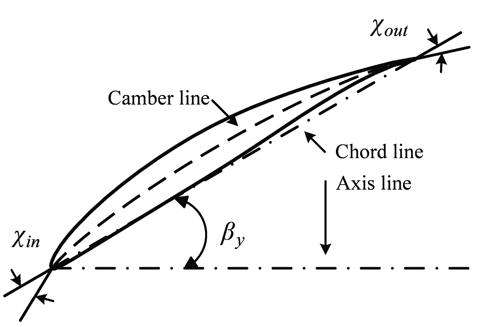
Eighteen geometric parameters were selected as design variables, as shown in

Table 1. Definitions and ranges of the design variables.

Variable	Definition	Ref	Min	Max	Variable	Definition	Ref	Min	Max
$d{m}_1/c_0$	$dm$ at $\widehat{r}=1/3$	0	−0.07	0.07	${\chi }_{in,4}/\mathrm{rad}$	${\chi }_{in}$ at $\widehat{r}=1$	0.050	−0.05	0.15
$d{m}_2/c_0$	$dm$ at $\widehat{r}=2/3$	0	−0.14	0.14	${\chi }_{out,1}/\mathrm{rad}$	${\chi }_{out}$ at $\widehat{r}=0$	−0.640	−0.67	−0.6
$d{m}_3/c_0$	$dm$ at $\widehat{r}=1$	0	−0.21	0.21	${\chi }_{out,2}/\mathrm{rad}$	${\chi }_{out}$ at $\widehat{r}=1/3$	−0.052	−0.08	−0.02
$d{\theta }_1/{\theta }_0$	$d\theta$ at $\widehat{r}=1/3$	0	−0.03	0.03	${\chi }_{out,3}/\mathrm{rad}$	${\chi }_{out}$ at $\widehat{r}=2/3$	−0.050	−0.08	−0.018
$d{\theta }_2/{\theta }_0$	$d\theta$ at $\widehat{r}=2/3$	0	−0.06	0.06	${\chi }_{out,4}/\mathrm{rad}$	${\chi }_{out}$ at $\widehat{r}=1$	−0.149	−0.18	−0.12
$d{\theta }_3/{\theta }_0$	$d\theta$ at $\widehat{r}=1$	0	−0.09	0.09	${\beta }_{y,1}/\mathrm{rad}$	${\beta }_y$ at $\widehat{r}=0$	0.224	0.18	0.26
${\chi }_{in,1}/\mathrm{rad}$	${\chi }_{in}$ at $\widehat{r}=0$	0.448	0.41	0.48	${\beta }_{y,2}/\mathrm{rad}$	${\beta }_y$ at $\widehat{r}=1/3$	0.656	0.6	0.7
${\chi }_{in,2}/\mathrm{rad}$	${\chi }_{in}$ at $\widehat{r}=1/3$	0.123	0.1	0.15	${\beta }_{y,3}/\mathrm{rad}$	${\beta }_y$ at $\widehat{r}=2/3$	0.965	0.92	1
${\chi }_{in,3}/\mathrm{rad}$	${\chi }_{in}$ at $\widehat{r}=2/3$	0.064	−0.04	0.16	${\beta }_{y,4}/\mathrm{rad}$	${\beta }_y$ at $\widehat{r}=1$	1.099	1.05	1.15

, where $\widehat{r}$ is the unidimensional radius, and $c_0$ and ${\theta }_0$ are constants to normalize $dm$ and $d\theta$, with $c_0$ = 9.561 cm and ${\theta }_0$ = 0.286 rad. The design variables were used as control points in the 3-order Bezier curve to generate the span distributions of $dm(r_a)$ and $d\theta (r_a)$, the inlet camber angle ${\chi }_{in}(r_a)$, the outlet camber angle ${\chi }_{out}(r_a)$, and incidence ${\beta }_y(r_a)$. Figure 3 shows the definitions of ${\chi }_{in}(r_a)$, ${\chi }_{out}(r_a)$ and ${\beta }_y(r_a)$, where the ${\chi }_{out}(r_a)<0$ because the counterclockwise direction was considered positive. The 2D airfoils changed as the ${\chi }_{in}(r_a)$ and ${\chi }_{out}(r_a)$ were selected as the design variable, while other features including chord length, leading edge and trailing edge thickness remained unchanged. The reference value was extracted from the original NASA rotor 67 geometry to set the lower and upper bounds.

2.2. CFD Method

2.2.1. CFD Tools

The commercial software package NUMECA was selected for CFD analysis. The NUMECA AutoGrid generated an O–H-structured grid according to the rotor geometry. Then, the NUMECA Fine Turbo and CFView were applied to solve the 3D RANS equation and post-process. All tools were automatically driven by the predefined scripts.

The viscous and inviscid fluxes were determined using second-order Jameson-type dissipation, and an explicit Runge–Kutta scheme was applied for time discretization. The RANS equation was closed by the Spalart–Allmara (S–A) model, which has been effectively validated and applied in transonic compressor rotors [34,35,36] together with NUMECA Fine Turbo.

2.2.2. Rotor 67 Simulation

NASA rotor 67 [19] is a low-aspect ratio, transonic, axial-flow fan rotor with abundant experimental data, and was selected as the reference design, with its primary features shown in

Table 2. Specification of rotor 67 [19].

Parameter	Value	Parameter	Value
Rotational speed (rpm)	16,043	Relative tip (Mach)	1.3
Tip clearance (cm)	0.101	Mass flow rate (kg/s)	33.25
Number of blades	22	Pressure ratio	1.63

. It should be noted that the observed tip clearance was 0.061 cm rather than the designed value of 0.101 cm [19].

Different grids were calculated with 0.8 M, 1.2 M, and 1.6 M nodes, and $y^{+}=1$ was specified for all grids. The O–H topology worked well in the single-stage rotor and generated good grids, as shown in Figure 4. As for boundary conditions, total pressure and temperature were specified at the inlet, and static pressure was specified at the outlet.

The calculated operating characteristics and the experimental results are plotted in Figure 5. It can be seen that the pressure ratio and efficiency fit the experimental data well for the medium (1.2 million) and fine (1.6 million) meshes, while the coarse mesh results deviated from the experimental values. The calculated chock mass flow rate was 34.3 kg/s, which is slightly less than the experimental value but was considered acceptable.

Since the rotor was simulated in the steady state but the rotating stall was an unsteady process, the time-averaged features and convergence criteria can be used to approximate the numerical stall point [18,37,38]. The calculation converged if the adiabatic efficiency variation was less than 0.04% per 100 iterations, and the calculation was regarded as stalled if the CFD case did not converge. The calculated stall mass flow was 93% in both the 1.2 million and 1.6 million grids. Besides this, the calculated shock wave showed similar features to the experiment shock wave.

The CFD result of the pressure and temperature ratio distributions fits the experimental result well with a deviation of less than 3.27%, as plotted along the spanwise direction at near-peak efficiency in Figure 6. Thus, the CFD tools and methods provide reliable results, and these approaches were then applied to generate and evaluate the agent-generated rotor geometries. The design space was considered based on rotor 67, so the obtained results may share similar characteristics, and the CFD methods above can give reliable results.

2.2.3. Rotor Performance Specification

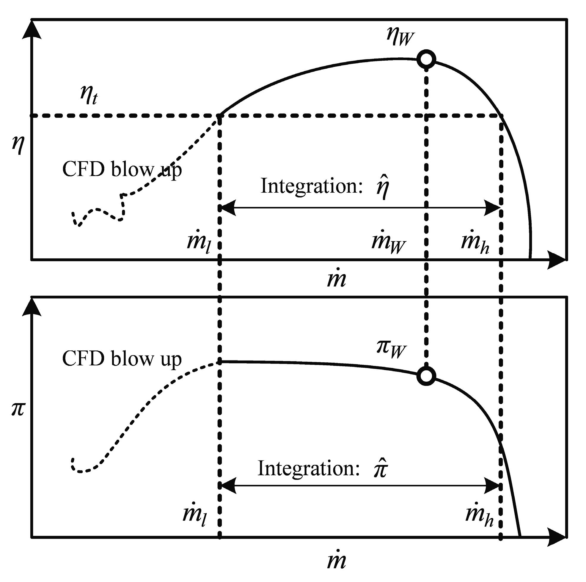
The most important performance variables for a compressor were the mass flow $\dot{m}$, pressure ratio $\pi$, efficiency $\eta$, and stability margin $SM$. A typical operating characteristic curve generated by the CFD method is shown in Figure 7, in which the back pressure $p_{out}$ was changed according to a geometric distribution. The peak efficiency point was selected as the working point, and the mass flow ${\dot{m}}_W$, pressure ratio ${\pi }_W$, and efficiency ${\eta }_W$ can also be determined simultaneously.

Furthermore, several variables were defined to evaluate the operating characteristic curve. An efficiency range $[{\dot{m}}_l,{\dot{m}}_h]$ was defined after setting an efficiency threshold ${\eta }_t$, as shown in Figure 7. The variables included the numerical stall feature of the rotors, so these features were used instead of the exact stall point during agent training, which reduced the required computational resources.

The integral efficiency $\widehat{\eta }$ and pressure ratio $\widehat{\pi }$ are defined as Equations (1) and (2) in order to take the shape of the operating characteristic curve into account, which evaluates the performances in the range $[{\dot{m}}_l,{\dot{m}}_h]$. The rotor performance included seven variables, denoted by $p_i\in \mathbb{P}=\{{\dot{m}}_l,{\dot{m}}_h,\widehat{\eta },\widehat{\pi },{\dot{m}}_W,{\pi }_W,{\eta }_W\}$, i = 1, 2, …, and 7, respectively.

$$\widehat{\eta }=\frac{{\displaystyle \underset{{\dot{m}}_l}{\overset{{\dot{m}}_h}{\int }}\eta (\dot{m})d\dot{m}}}{{\dot{m}}_h-{\dot{m}}_l}$$

(1)

$$\widehat{\pi }=\frac{{\displaystyle \underset{{\dot{m}}_l}{\overset{{\dot{m}}_h}{\int }}\pi (\dot{m})d\dot{m}}}{{\dot{m}}_h-{\dot{m}}_l}$$

(2)

2.3. Modified DDPG Algorithm

The DDPG algorithm [30] is a model-free and off-policy approach that can robustly address challenging problems in continuous state spaces, including high-dimensional problems. Therefore, the DDPG algorithm is appropriate for application in compressor design optimization. The Adam optimizer [39] and L2 normalization were applied when implementing the DDPG algorithm. The environmental reward was defined by the rotor performance variables $p_i\in \mathbb{P}$.

2.3.1. Modifications to Improve the DDPG Algorithm

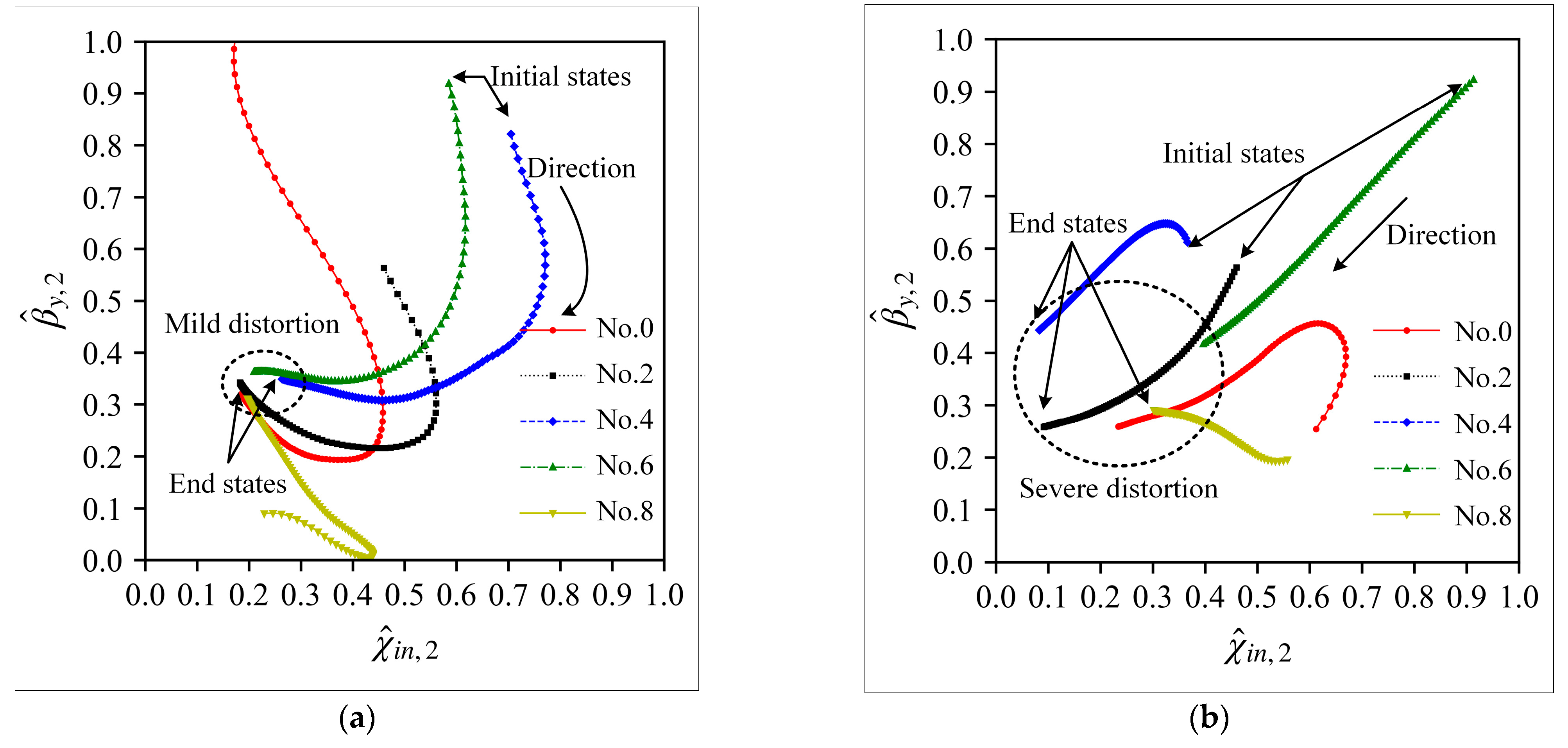
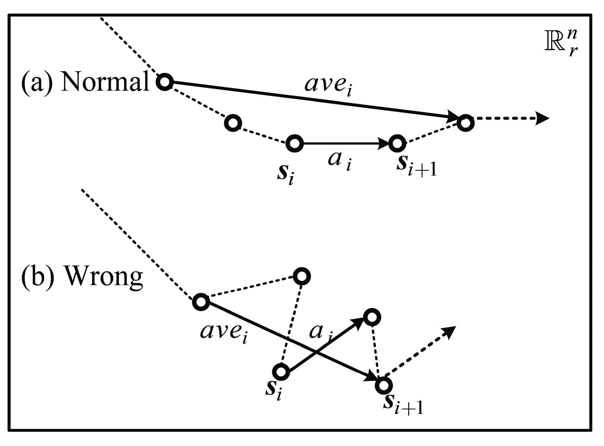
It was observed that the end states of MDPs dispersed to different degrees, and this dispersion was considered as distortion. Two agents with similar accumulated rewards R were compared, as shown in Figure 8, in which the agents acted in the real design space ${ℝ}_r^n$ and generated the state sequences. The sequences started with different initial states and ended at the states in dashed circles, with the directions also marked out. A server distortion was found in Figure 8b, while the distortion in Figure 8a was relatively mild. Since the design space and performance are highly dimensional, this distortion cannot be eliminated easily. This feature has also been observed in other studies [40] using the DDPG algorithm. Agents with severe distortion cannot guide the design process; thus, three modifications were applied to reduce the distortion and improve the training speed.

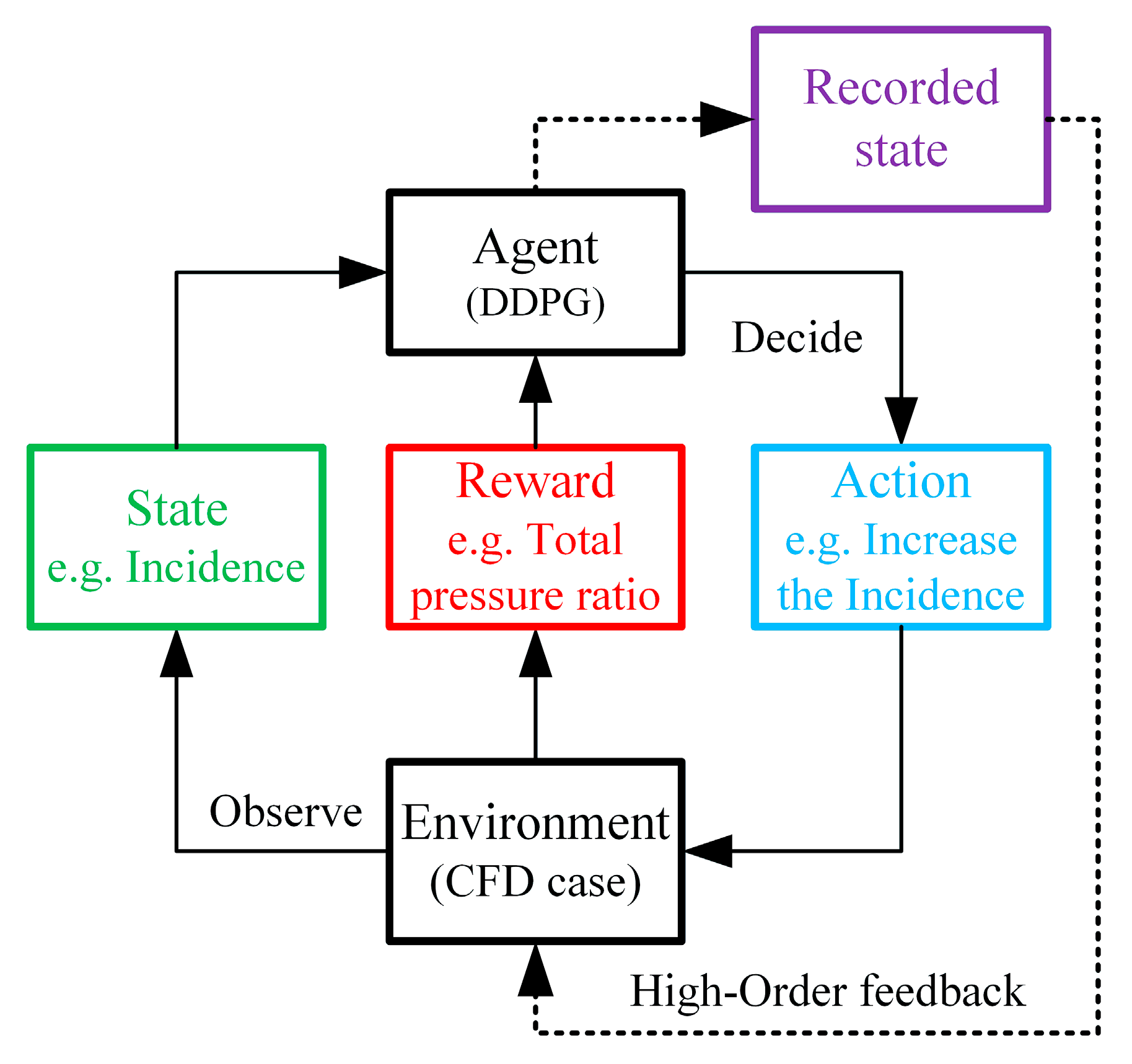
High-order feedback was applied to guide the exploration, as shown in Figure 9. The agent determined an action according to the state, and then interacted with the environment. The state was the design variable—for example, one of the state dimensions was the incidence—and the action was the corresponding modification, such as an increase in the incidence. Unlike the other RL question, the initial state in the rotor design was configurable, so the agent was expected to explore more rigorously near the detected optimized state, and the best state $s^{*}$ in the environment was updated in each test process.

Then, as a part of high-order feedback, Randomness was added to enhance the exploration. The initial states were selected near $s^{*}$ with random directions ${\overrightarrow{n}}_{rand}$ and deterministic radii $R_{const}$, as shown in Equation (3). This method ensured that the initial states were sufficiently similar to the recorded optimized state.

$$s_o=s^{*}+{\overrightarrow{n}}_{rand}•R_{const}$$

(3)

A virtual area was added to extend the design space so the agents could obtain more transitions $(s_t,a_t,r_t,s_{t+1})$ near the boundary. The agent stopped exploring when it exited the design space ${ℝ}_r^n$, hence the transitions reduced near the boundary. This reduction was considered one of the main reasons for the distortion observed in Figure 8, and could be resolved by adding the virtual area.

The real design space ${ℝ}_r^n$ and the virtual area ${ℝ}_v^n$ are shown in Figure 10. The correct reward term $\delta r_{vir}$ was nonzero if the state was in ${ℝ}_v^n$, and zero if the state was in ${ℝ}_r^n$. d refers to the Manhattan distance between $s_v\in {ℝ}_v^n$ and ${ℝ}_r^n$. The constant $c_V=-0.3/dx$ ensured that $\delta r_{vir}\le 0$, which guaranteed that the maximum reward state was in ${ℝ}_r^n$.

An artificial tip was utilized to improve the gradient near the $s^{*}$ and accelerate the training by defining an additional correct term $\delta r_{art}$ in Equation (4), where ${\delta }_s$ and $d{r}_0$ were constants and $d{r}_0=0.08$ in this study. The $\delta r_{art}$ did not change the monotonicity of the reward $r(s)$ or the location of $s^{*}$, and increased the gradient.

$$\delta r_{art}=\left\{\begin{array}{ll}0& ‖s-s^{*}‖\ge {\delta }_s\\ d{r}_0& ‖s-s^{*}‖\le {\delta }_s\end{array}\right.$$

(4)

2.3.2. Environment Definition

The RL environment was coded following the template of OpenAI Gym. The state of the environment was the design variable $s\in \mathbb{S}$, as discussed in Section 2.1. The aerodynamic performance variables $p_i\in \mathbb{P}$, i = 1, 2, …, and 7 were generated by the surrogate models. The reward in the environment was defined by $p_i$, as shown in Equation (5).

$$r=a_1{r}_{raw}+a_2+{\displaystyle \sum _{p_i\in \mathbb{P}}\delta r_{p_i}}+\delta r_{art}+\delta r_{vir}$$

(5)

where $r_{raw}$ was a function of the different $p_i$ variables that determines what the agents are expected to learn. $a_1$ and $a_2$ were constants used to scale $r_{raw}$. $\delta r_{art}$ and $\delta r_{vir}$ were the correct reward terms for the artificial tip and virtual area. This general reward form guaranteed that different $r_{raw}$ definitions could be solved universally, which benefited the agent training and improved the general applicability of the methodology.

The punishment term $\delta r_{p_i}$ was defined in Equation (6) as a constraint on each performance variable $p_i$. $\delta r_{0,i}$ and $w_i$ determined the strength of the constraint, and $\delta p_i=\min (\left|p_i-p_{cl,i}\right|,\left|p_i-p_{cu,i}\right|)$ indicates how much $p_i$ exceeded its reasonable range $[p_{cl,i},p_{cu,i}]$, which was defined according to the performance of the reference rotor. The weightings $w_i$ can be determined to balance the $\delta p_i$ of different dimensions using the Monte Carlo method.

$$\delta r_{p_i}=\left\{\begin{array}{cc}0& p_i\in [p_{cl,i},p_{cu,i}]\\ \delta r_{0,i}+\delta p_i\times w_i& p_i\notin [p_{cl,i},p_{cu,i}]\end{array}\right.$$

(6)

2.3.3. Policy Evaluation

The trained agents generated different design processes, and the states $s_i$ formed curves in the design space ${ℝ}_r^n$. The maximum number of steps has been denoted as $N_p$, so i = 1, 2, …, $N_p$. In addition to the accumulated reward R, two additional criteria were defined to evaluate the policy.

First, the consistency criterion was defined to evaluate the distortion at the end of the process. The consistency criterion ${\epsilon }_d$ is defined in Equation (7), where $s_{end,j}$ is the end state of the jth process among the $N_p$ test processes with random initial states. Lower ${\epsilon }_d$ values indicate more successful training.

$${\epsilon }_d=\frac{1}{N_p}{\displaystyle \sum _{j=1}^{N_p}‖s_{end,j}-\frac{1}{N_p}{\displaystyle \sum _{k=1}^{N_p}{s}_{end,j}}‖}$$

(7)

Then, the smoothness criterion was defined to filter incorrect policies. The agents may obtain the wrong policy and generate zigzag curves, as shown in Figure 11. This phenomenon might occur because the actor networks are overfitted on the recorded transactions, and this can be prevented by adjusting the hyperparameters. Agents with incorrect policies cannot guide the design and should be removed.

The smoothness criterion ${\epsilon }_c$ was defined according to the angles of $a_i$ and $av{e}_i$, as shown in Equation (8), where $s_i$ and $a_i$ are the transaction state and action, $n_w$ indicates the number of states used to calculate ${\epsilon }_c$, and $av{e}_i$ is the sum of the $2n_w+1$ steps near $s_i$. ${\epsilon }_c$ was closer to 1 if the agent learned a good policy.

$${\epsilon }_c=\frac{1}{N-2n_w-1}{\displaystyle \sum _{i=1+n_w}^{N-n_w}\frac{\left|a_i•av{e}_i\right|}{‖a_i‖•‖av{e}_i‖}}$$

(8)

The three modifications were tested in a demo case to verify the effectiveness of reducing ${\epsilon }_d$. As shown in Equation (9), the reward in the demo case was defined by the distance from a selected extreme point $s_0$, $s\in {ℝ}^2$, $d(s,s_0)=‖s-s_0‖$, $d_{max}(s_0)=\max (d(s,s_0))$, and the constant $p_c$ defined the shape of the tip.

$$r(s,s_0)=\frac{p_c}{\raisebox{1ex}{$d(s,s_0)$}\!\left/ \!\raisebox{-1ex}{$d_{max}(s_0)$}\right.+p_c}$$

(9)

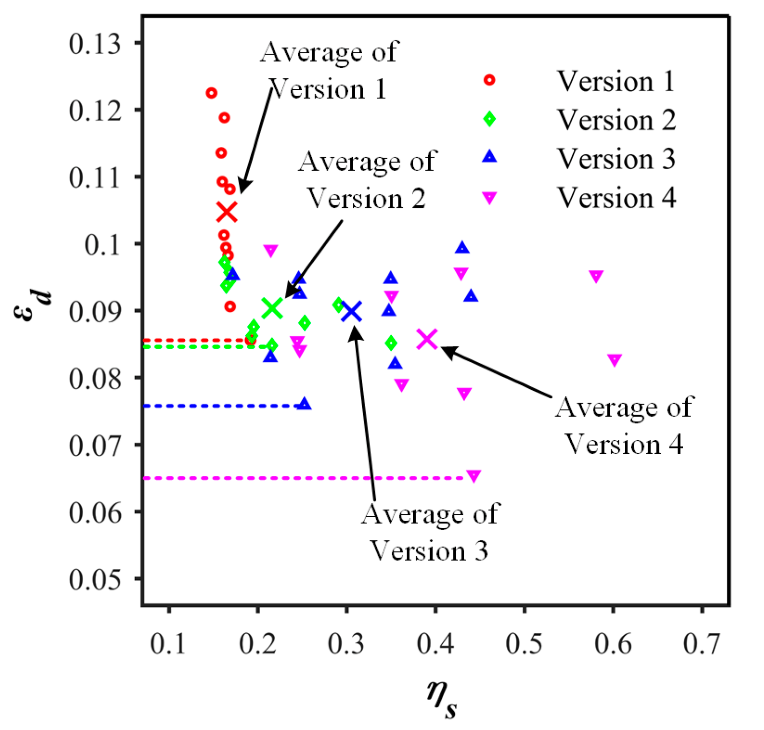
The agents were trained with $s_0=(0.3,1)$, which made the maximum point of the demo function near the boundary. Good ${\epsilon }_c$ values were obtained for all agents, and the consistency criterion ${\epsilon }_d$ was monitored. The training speed was evaluated by ${\eta }_s=R/N_{ep}$, where R was the accumulated reward and $N_{ep}$ was the number of training episodes.

The agents in four different configurations were trained 10 times and stopped when $R>85$ or $N_{ep}>500$, as shown in Figure 12. Version 1 used the original DDPG algorithm, and version 2 included the virtual grid. Version 3 included both high-order feedback and the virtual grid, and version 4 included all three modifications. When the modifications were applied, the average and minimum ${\epsilon }_d$ values decreased, and the ${\eta }_s$ value increased, showing that the performance of the modified algorithms was better than that of the original DDPG algorithm.

2.4. Error-Reduced Kriging Model

Surrogate models provide accurate approximations in CFD analyses with considerably reduced computational costs, which accelerates the design process. The 3D rotors had more design variables than 2D airfoils, and their CFD analyses require more computational resources, increasing the difficulty of establishing surrogate models.

2.4.1. Kriging Model

The kriging model [41] needs few sample points, even in high-dimensional design spaces; thus, this model has been widely applied in compressor design [9]. This work used kriging models to approximate rotor performance and the maximin Latin hypercube design [42] to find the sample points.

$${\psi }^{(i)}=\exp \left(-{\displaystyle \sum _{j=1}^k{\theta }_j{\left|s_j-{s_j}^{(i)}\right|}^{P_j}}\right)$$

(10)

As a radial basis function (RBF) model, the number i RBF ${\psi }^{(i)}$ is expressed by Equation (10), where $s_j$ and ${s_j}^{(i)}$ are the components of variable $s$ and sample point $s^{(i)}$, and $k$ is the dimension number. The kriging model included parameters ${\theta }_k={\left\{{\theta }_1,{\theta }_2,\dots ,{\theta }_k\right\}}^T$ and $P_k={\left\{P_1,P_2,\dots ,P_k\right\}}^T$, and the number of parameters depended on the dimension of the design variable and the number of sample points. A PSO algorithm was applied to determine the kriging parameters by maximizing the likelihood function of the sample point’s value. Larger $P_k$ and smaller ${\theta }_k$ values increased the smoothness of RBF, so fewer sample points were needed when decreasing ${\theta }_k$ and increasing $P_k$.

Seven kriging models were trained to approximate the performance of the rotor. It was assumed that the basis functions were sufficiently smooth, so the ranges of ${\theta }_k$ and $P_k$ were limited. Combined with the error reduction process, the accuracy of the surrogate models improved.

2.4.2. Error Reduction

The error reduction process was implemented to enhance the performance of the kriging model and reduce the number of required samples. The basic idea of the error reduction process was to reduce the influence of extreme sample points.

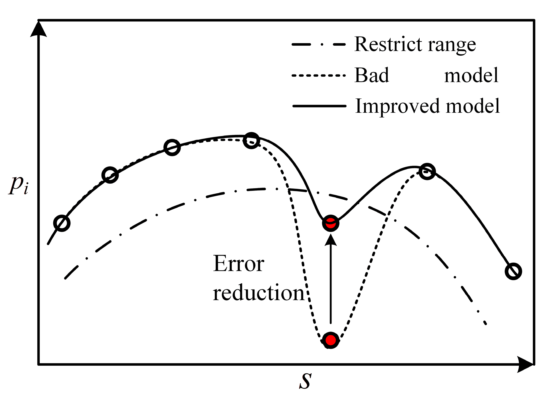
The sample points with poor aerodynamic performance did not substantially influence the design, but they deteriorated the performance of surrogate models, because these points may be outliers with a lower reward. Therefore, sample points with poor aerodynamic performance were restricted by a preset reasonable range to improve model accuracy, as schematized in Figure 13. If a sample point obtained a performance outside this range, the sample point was forced to move toward the reasonable range. This process reduced the error between the sample point and the range, thereby improving model performance.

If the performance $p_i\in \mathbb{P}$ exceeded the reasonable range $[p_{i,min},p_{i,max}]$, the excessive part was reduced. For example, the unidimensional exceeding term $\delta \widehat{p_i}$ can be defined as in Equation (11) if $p_i>p_{i,max}$ and $\delta \widehat{p_i}$ became $\delta \widehat{{p_i}^{\prime }}$ after applying a logarithmic restriction in Equation (12). The parameter $a_p$ indicates the strength of the restriction, where $a_p>0$. In view of the computational cost and necessity, the candidate values were $a_p\in \left\{0,\hspace{0.33em}3,\hspace{0.33em}5\right\}$, and they are tested in Section 2.4.3.

$$\delta \widehat{p_i}=\frac{p_{i,max}-p_i}{p_{i,max}-p_{i,min}}>0$$

(11)

$$\delta \widehat{{p_i}^{\prime }}=\frac{1}{a_p}\ln (a_p\delta \widehat{p_i}+1)$$

(12)

Then, the restricted performance ${p_i}^{\prime }$ was reconstructed using the restricted exceeding term $\delta \widehat{{p_i}^{\prime }}$, as shown in Equation (13). $\delta \widehat{{p_i}^{\prime }}$ maintained the monotonicity of $\delta \widehat{p_i}$ and the first–order smoothness. The restriction did not work if the $p_i$ was less than the threshold. Then, the more $p_i$ exceeded the threshold, the stronger the restriction was. The error reduction process was similar if $p_i<p_{i,min}$, and this significantly improved the performance of the surrogate model, as discussed in Section 2.4.3.

$${p_i}^{\prime }=p_{i,max}+\delta \widehat{p_i}\times (p_{i,max}-p_{i,min})$$

(13)

2.4.3. Surrogate Models for Rotors

NASA rotor 67 was selected as the reference design, and the design space is shown in Table 1. Sample points $s\in \mathbb{S}$ were selected to generate the geometry, calculate the operating characteristics and determine the performance variables $p_i\in \mathbb{P}$, i = 1, 2, …7. Then, the surrogate models were trained using the sample points generated by CFD tools.

The coefficient of determination $R^2$ was calculated to evaluate the trained surrogate models and has been defined in Equation (14), where $p_i\in \mathbb{P}$, i = 1, 2, …7 were the performance variables, $p_{i,j}$ and ${\widehat{p}}_{i,j}$ were the actual and predicted values of the jth test point, respectively, and ${\overline{p}}_i$ was the average value of all tested points.

$${R^2}_{p_i}=\frac{{\displaystyle \sum _{j=1}^{n_t}{(p_{i,j}-{\overline{p}}_i)}^2}}{{\displaystyle \sum _{j=1}^{n_t}{({\widehat{p}}_{i,j}-{\overline{p}}_i)}^2}}$$

(14)

The $R^2$ values of ${\pi }_w$ and $\widehat{\eta }$ with different numbers of sample points are shown in Figure 14. The surrogate models with and without the error reduction process were compared. The accuracy of the kriging models increased when applying the error reduction process. The improvement was obvious if the original surrogate models were less accurate, and decreased if the original models were sufficiently accurate.

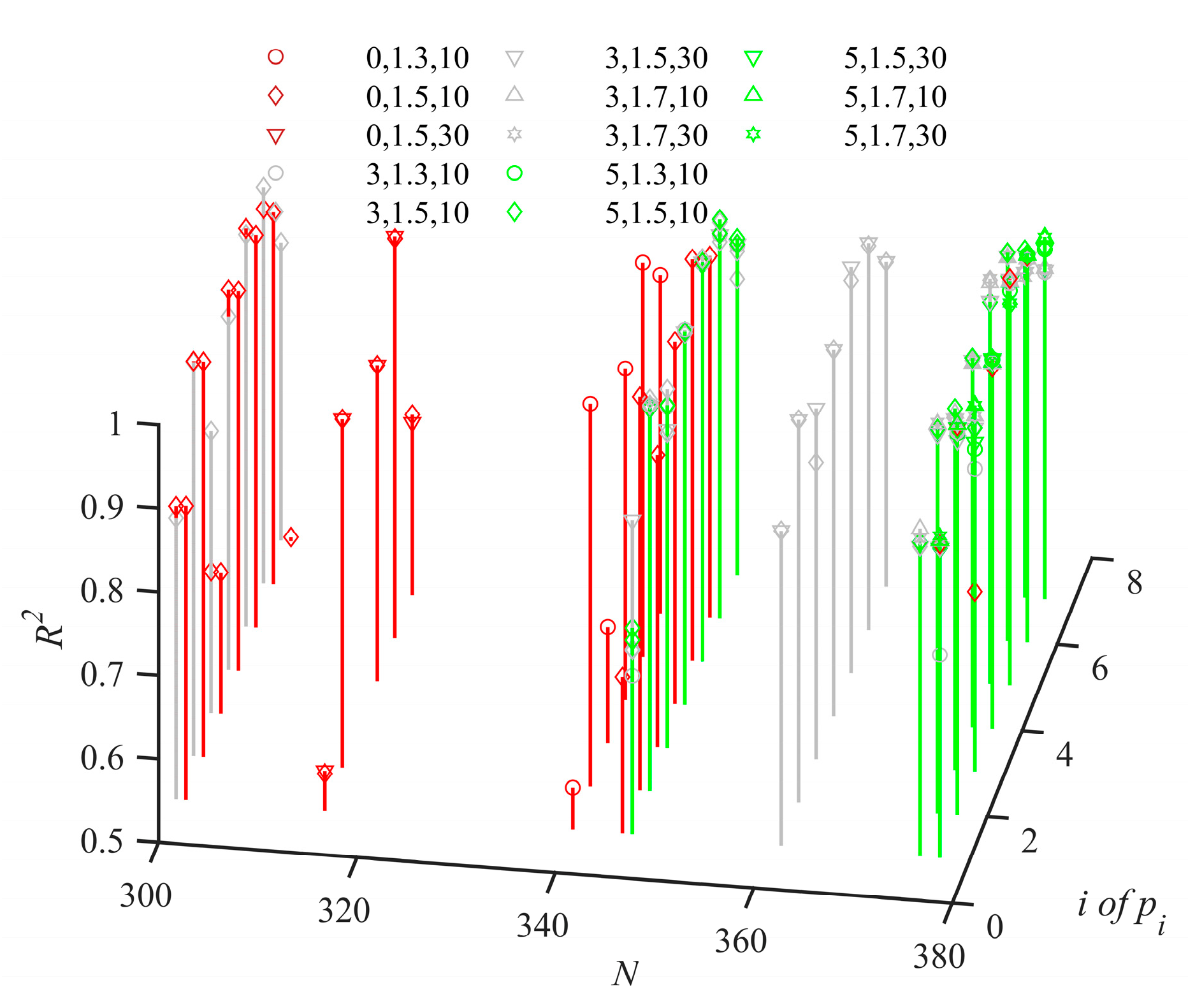
Finally, surrogate models with different performance variables $p_i$ were trained with various numbers of samples N, as shown in Figure 15. The combinations of different $a_p$, $p_{min}$ and ${\theta }_{max}$ are listed in the legend, with $a_p=0,3,5$ and ${\theta }_{max}=10,30$. In general, the models performed better when more sample points were included; the models for ${\dot{m}}_l$(i = 1), $\widehat{\eta }$(i = 3) and ${\pi }_W$(i = 7) showed poor performance when N was less than 360 if $a_p$=0, and improved after N increased. Each $p_i$ had its own distribution, and if the distribution was not smooth and N was large, larger $a_p$ values reduced the model performance. The models for ${\dot{m}}_W$(i = 5) obtained $R^2$=0.987 when $a_p$=0, which was 0.1% higher than the $R^2$ value obtained when $a_p$=3.

The best surrogate models for each $p_i$ were selected and are shown in

Table 3. Performances of different models.

${\mathit{p}}_{\mathit{i}}$	${\mathit{R}}^2$	$\mathit{M}\mathit{A}\mathit{E}$	$\mathit{N}$	${\mathit{a}}_{\mathit{p}}$	${\mathit{\theta }}_{\mathit{m}\mathit{a}\mathit{x}}$	${\mathit{P}}_{\mathit{m}\mathit{i}\mathit{n}}$
${\dot{m}}_l$	0.886	0.011	377	5	30	1.7
${\dot{m}}_h$	0.968	0.005	377	5	10	1.7
$\widehat{\eta }$	0.938	0.001	377	5	30	1.7
$\widehat{\pi }$	0.942	0.004	377	5	10	1.5
${\dot{m}}_W$	0.987	0.003	377	0	10	1.5
${\pi }_W$	0.965	0.001	377	5	10	1.5
${\eta }_W$	0.920	0.005	377	5	30	1.5

, where $R^2$ and mean absolute error (MAE) are also listed. The surrogate models accurately predicted the performance of the rotor; thus, a reinforcement learning environment was established based on these surrogate models.

3. Results

3.1. Policy for Improving the Pressure Ratio

The pressure ratio is an important compressor performance indicator. Improving the stage pressure ratio can reduce the compressor’s size and weight. Thus, in this section, the agents have been trained to improve the pressure ratio of the rotors, and they are denoted as “series 1” agents.

The integrated pressure ratio $\widehat{\pi }$ was selected to establish the reward function, with $r_{raw}=\widehat{\pi }-{\widehat{\pi }}_0$, where ${\widehat{\pi }}_0$ was the reference value, and then the reward function was determined according to Equation (5). The scaling and constraint parameters in Equation (5) were determined using the Monte Carlo method of three hundred random points to ensure that the reward r was approximately in the range $[0,1]$.

The trained agents successfully learned the design policy. After approximately 4000 training episodes, the accumulated total reward R improved significantly. The smoothness criterion ${\epsilon }_c$ and consistency criterion ${\epsilon }_d$ were also considered during agent training. The details of the training rules are discussed in Section 4.1.

The agents started the design process in the reference state and modified all the design variables simultaneously to improve the pressure ratio. The nondimensionalized design variables are plotted in Figure 16, showing that the modification was noticeable in the first few steps, and then the change slowed. The policy learned by the agents was relatively complex, because the design variables at different spanwise distances showed distinct modifications. For example, ${\chi }_{out,1}$ increased, while ${\chi }_{out,2}$ and ${\chi }_{out,3}$ decreased, and some design variables, such as $d{m}_{r,1}$ and ${\chi }_{in,2}$, showed little change.

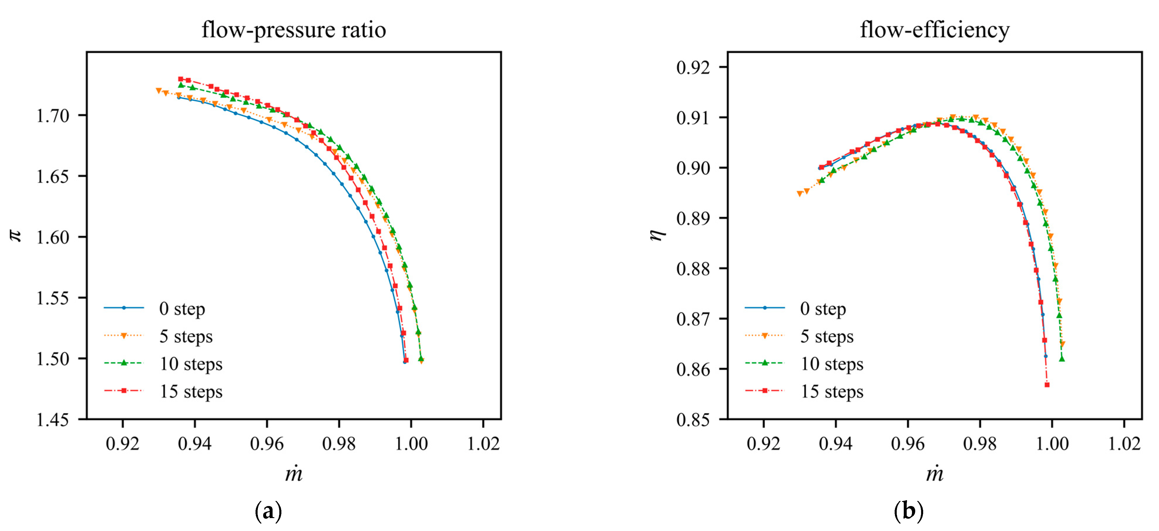
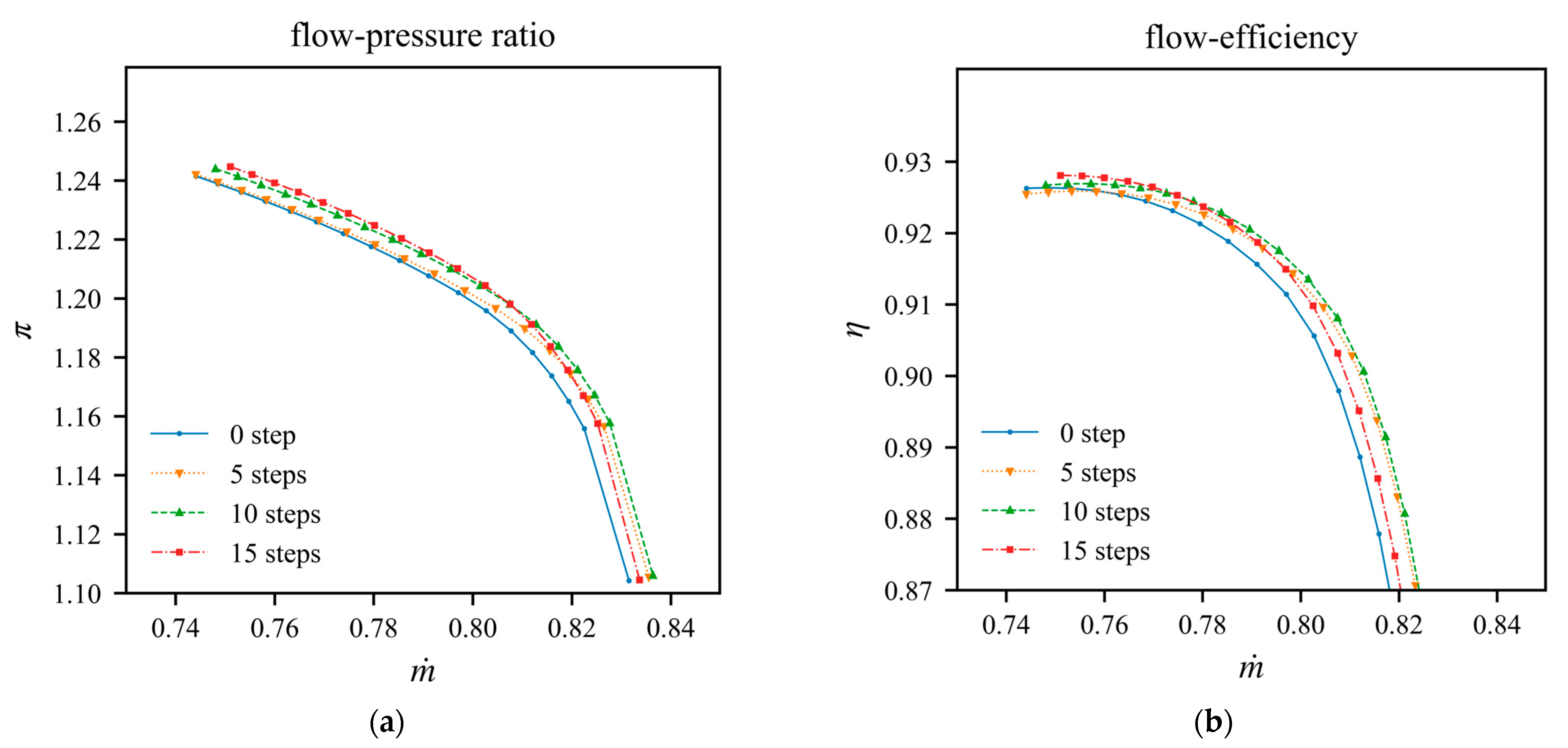
Figure 17 showed the operating characteristic curves of the rotors after the modification was applied. The pressure ratio improved with the number of steps and the efficiency improved in the first ten steps, showing that the RL environment constraints worked well. Then, as the agent attempted to further improve the pressure ratio, the efficiency deteriorated. The chock and near-peak efficiency mass flow also increased in the first ten steps, and then decreased; thus, the flow-efficiency curves nearly coincide at steps 0 and 15. In addition, the near-stall mass flow of the modified rotors was not worse than that of the original rotor.

The peak performance, chock mass flow rate and pressure ratio improved, as shown in

Table 4. Performances of modified rotors at different steps.

Step Number	${\dot{\mathit{m}}}_{\mathit{W}}$	${\mathit{\eta }}_{\mathit{W}}$	${\mathit{\pi }}_{\mathit{W}}$	$\mathit{\delta }{\mathit{\pi }}_{\mathit{W}}$
0	33.21	0.909	1.679	0
5	33.35	0.910	1.683	0.24%
10	33.44	0.910	1.686	0.41%
15	33.21	0.909	1.696	1.01%

. For the modified rotor, after 15 steps, ${\dot{m}}_W$ and ${\eta }_W$ were approximately equal to the reference values, and ${\pi }_W$ increased by 1.01%. The flow details are analyzed in Section 3.2. The agent could further improve the pressure ratio if a slight decrease in ${\eta }_W$ was accepted.

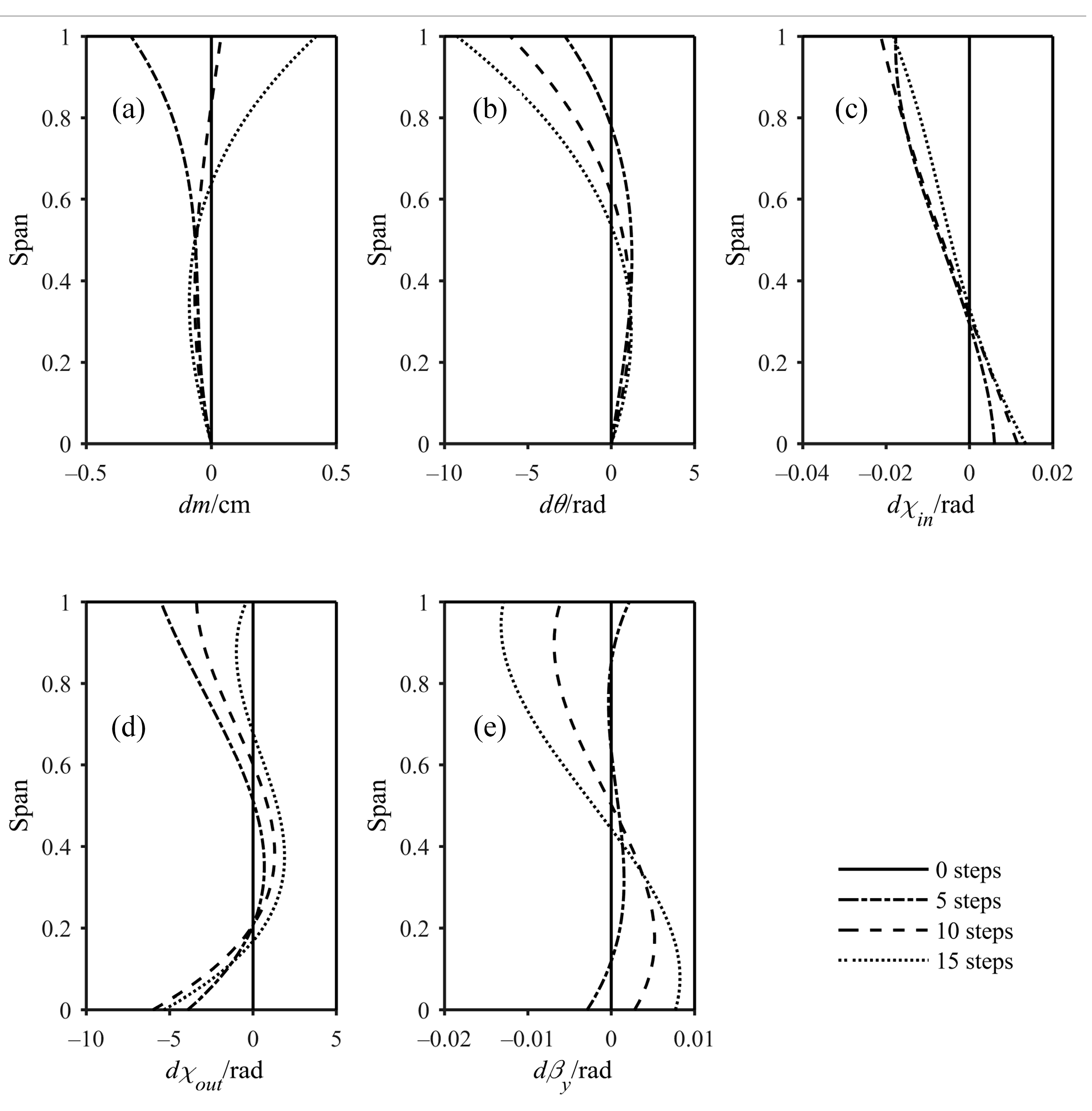
The variations in the geometric parameters $m$, $\theta$, ${\chi }_{in}$, ${\chi }_{out}$ and ${\beta }_y$ in the spanwise direction are plotted in Figure 18. The agents introduced a combined forward–back sweep feature, whereby the forward sweep feature was introduced in the middle section in the first five steps, and extended to approximately the whole span. The back sweep feature was introduced in the tip region. The blade lean feature was added with positive $d\theta$, and also diminished near the tip. The airfoil segment angle $\mathrm{\Delta }\beta$ increased in the middle span and decreased in the tip and hub regions as a result of the changes in ${\chi }_{in}$ and ${\chi }_{out}$. In addition, ${\beta }_y$ decreased near the tip and increased near the hub.

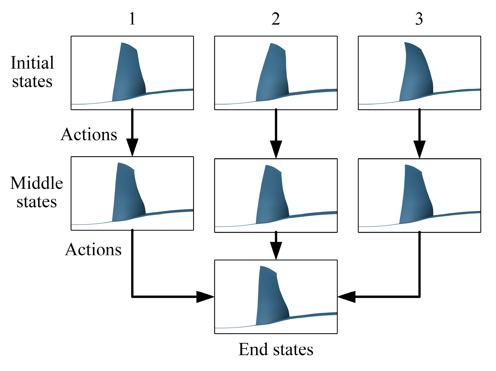
The trained agents could start the design in different initial states and modified the design very quickly, requiring only a few seconds to determine the action for a given state. As shown in Figure 19, the excessive forward sweep in the second initial geometry and the excessive back sweep in the third initial geometry were removed in the first few steps. Then, after a sufficient number of steps, the geometries approached the same final states.

3.2. Flow Field Analysis

After the series 1 agents modified the design variables, the flow field and model performance changed. An analysis of the flow mechanisms shows that the policy learned by the agents was effective and interpretable.

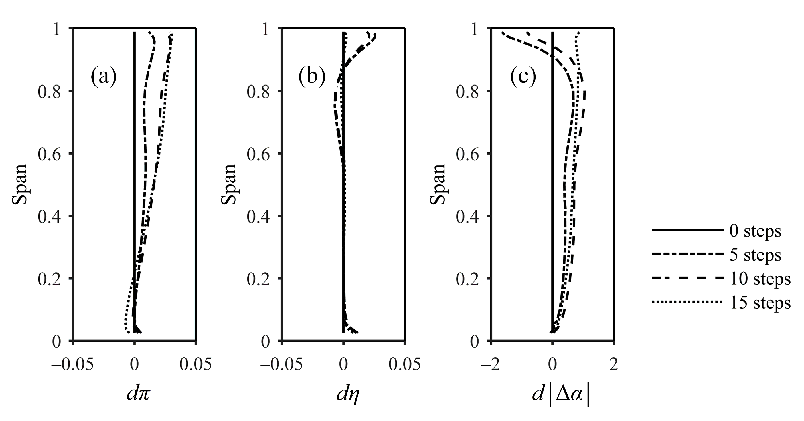
The deviations of the absolute flow angle $\mathrm{\Delta }\alpha$, local pressure ratio $\pi$, and local efficiency $\eta$ are plotted in Figure 20. $\mathrm{\Delta }\alpha$ increased in the middle span after ${\chi }_{in}$ and ${\chi }_{out}$ were modified, and the local pressure ratio $\pi$ also increased. Extra diffusion increased the $\pi$, and the boundary layer loss increased, so the $\eta$ decreased at approximately 80% span. Correspondingly, the local efficiency increased near the tip and hub, which compensated for the loss in the middle span; thus, the overall efficiency can be maintained at a relatively high level.

Zheng and Li [43] summarized that the forward sweep of rotor blades could improve the efficiency and the stable operating range. The sweep reduced the shock loss and the pressure increase in the rotors by changing the shape of the passage shock. As a result, extra pressure increases could be gained following diffusion, generating additional losses. Denton and Xu [44] affirmed that the shock waves in the tip region of the transonic rotor have a considerable impact on the pressure ratio. However, a shock wave that is too strong can cause excessive losses.

Figure 21 shows the isentropic Mach number along the chord in the 70% and 90% spanwise directions. The peak isentropic Mach number of the suction surface decreased after agent modification. After 15 steps, the isentropic Mach number increased a little, but was still no worse than the reference. Therefore, the angle change and the sweep weakened the shock wave, even with an increased pressure ratio. The isentropic Mach number of the pressure ratio near the leading edge decreased because ${\chi }_{in}$ changed more than ${\beta }_y$. The trained agent learned an excellent balance between the sweep and diffusion, and thus improved the $\pi$ and $\eta$ of the rotors.

Denton and Xu [45] noted that the pressure gradient perpendicular to the end wall must be zero. For this reason, the back sweep at the blade’s tip reduces the load at the trailing edge near the shroud. As shown in Figure 22, the load reduction and the change in the airfoil segment angle reduced the separation near the tip. After 15 steps, the back sweep and the change in airfoil segment angle decreased slightly. As a result, the separation was higher, but less than that at 0 steps, guaranteeing the efficiency of the rotors at the tip.

According to Sasaki and Breugelmans [46], because the lean angle between the end wall and the suction surface was obtuse, unloading occurred near the end wall, while overloading occurred near the mid-span. Shang et al. [47] explain the mechanism using the pressure gradient generated by the lean feature. The positive lean increased the static pressure of the suction surface, then the pressure gradient, especially after the throat location, drove the low-energy flow away from the corner. The trained agent learned to increase dθ, introducing a similar lean feature into the rotors.

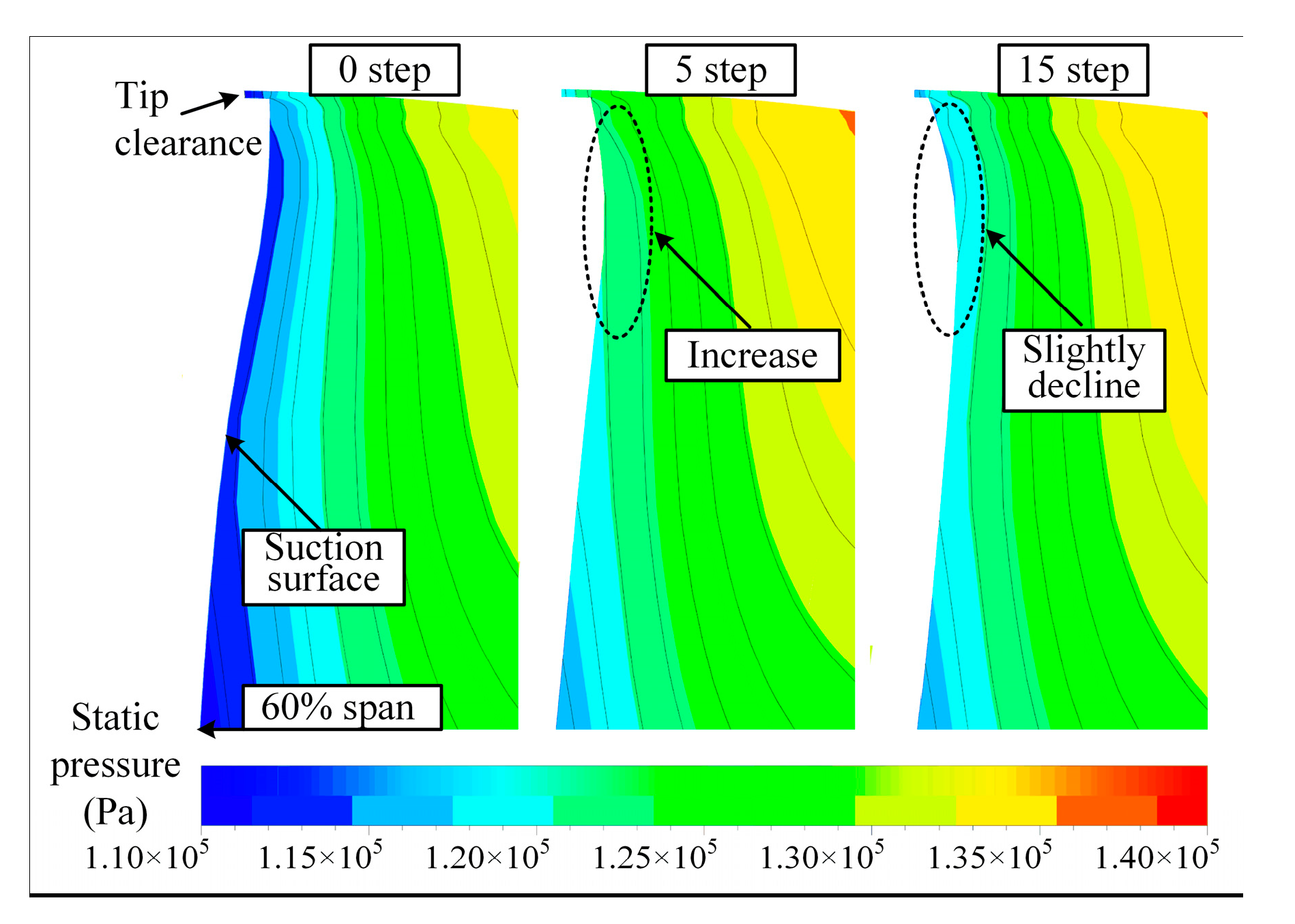
The static pressure distributions in the near–tip region at 80% axial length are compared in Figure 23. The static pressure increased in the tip region after agent modification. The pressure gradient drove the low-energy flow away from the corner, preventing the accumulation of the low-energy flow and reducing the separation. A change in the static pressure distribution occurred due to both the lean feature and the change in ∆β at the rotor tip.

The pressure difference between the pressure and suction surfaces drove the tip leakage flow and formed a tip leakage vortex (TLV). The geometry modifications influenced the TLV by changing the pressure difference between the pressure and suction surfaces.

The static pressure of the near-tip section (90% span) and near the tip clearance region (99.8% span) are plotted in Figure 24. The load at the leading edge near the tip increased because of the sweep and angle design, increasing the pressure difference at the leading edge. Then, the pressure difference of the modified rotors decreased after the 0.6 chord length. The minimum static pressure of the suction surface increased, and its location moved toward the leading edge, decreasing the inverse pressure gradient, which reduced the separation.

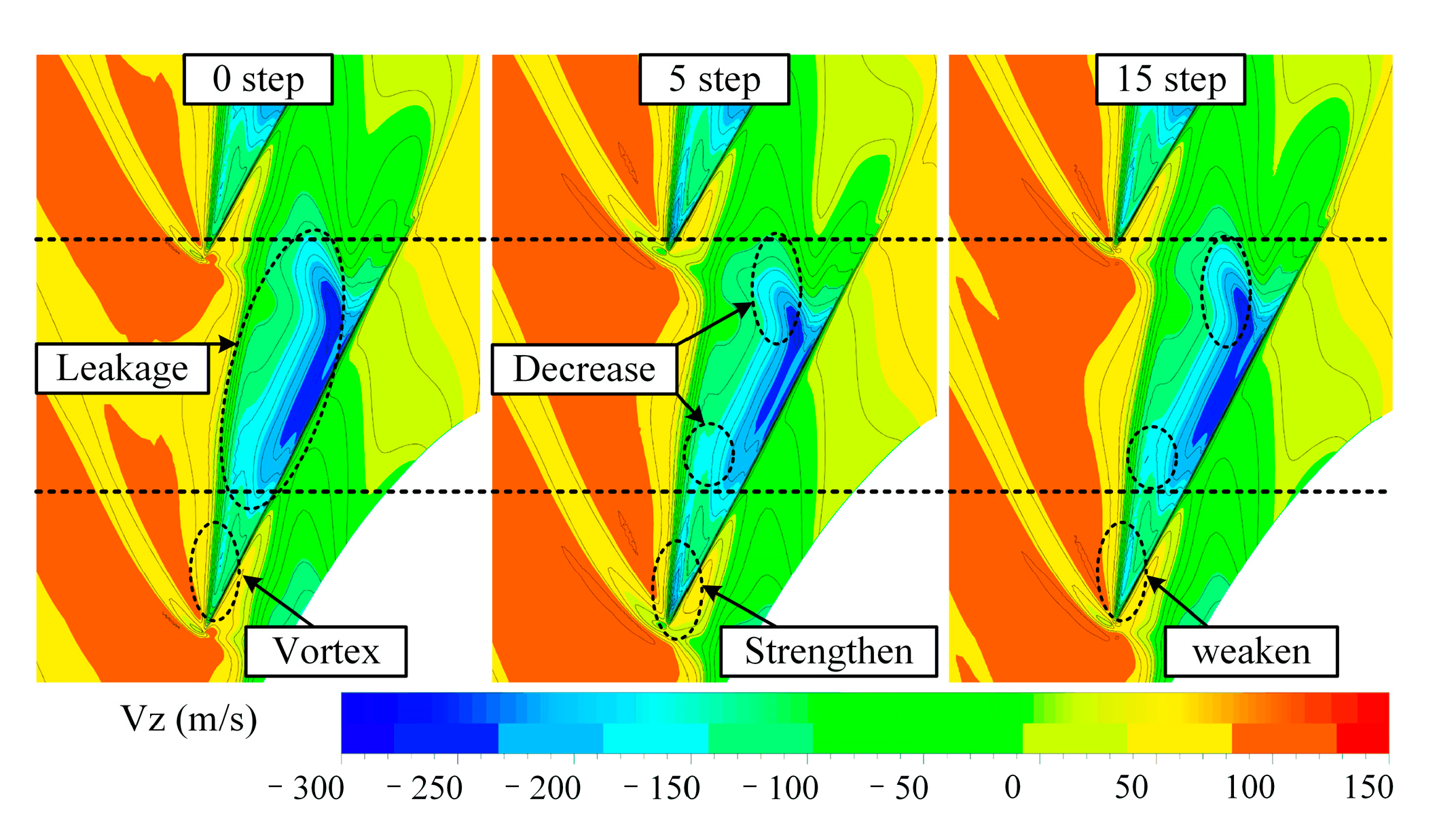
Chima [48] noted that the strength of the TLV depends on the chordwise integration pressure difference. Consequently, the TLV of modified rotors developed slowly and was weakened, even with a stronger initial strength at the leading edge. The axial velocity of the rotors at the tip clearance (99.8% span) is shown in Figure 25. The reference lines indicate that the TLVs in the modified geometries were stronger near the leading edge, but developed slower, and therefore the influence of the TLV was reduced.

Suder and Celestina [49] illustrated that the interaction between the TLV and the shock wave caused considerable losses. If the TLV crosses the passage shock, severe diffusion occurs, generating low-energy fluid because of the pressure rise caused by the shock wave. Then, the low-energy fluid mixes with the main flow, increasing the loss. The low-energy fluid also blocks the flow and influences the stall margin.

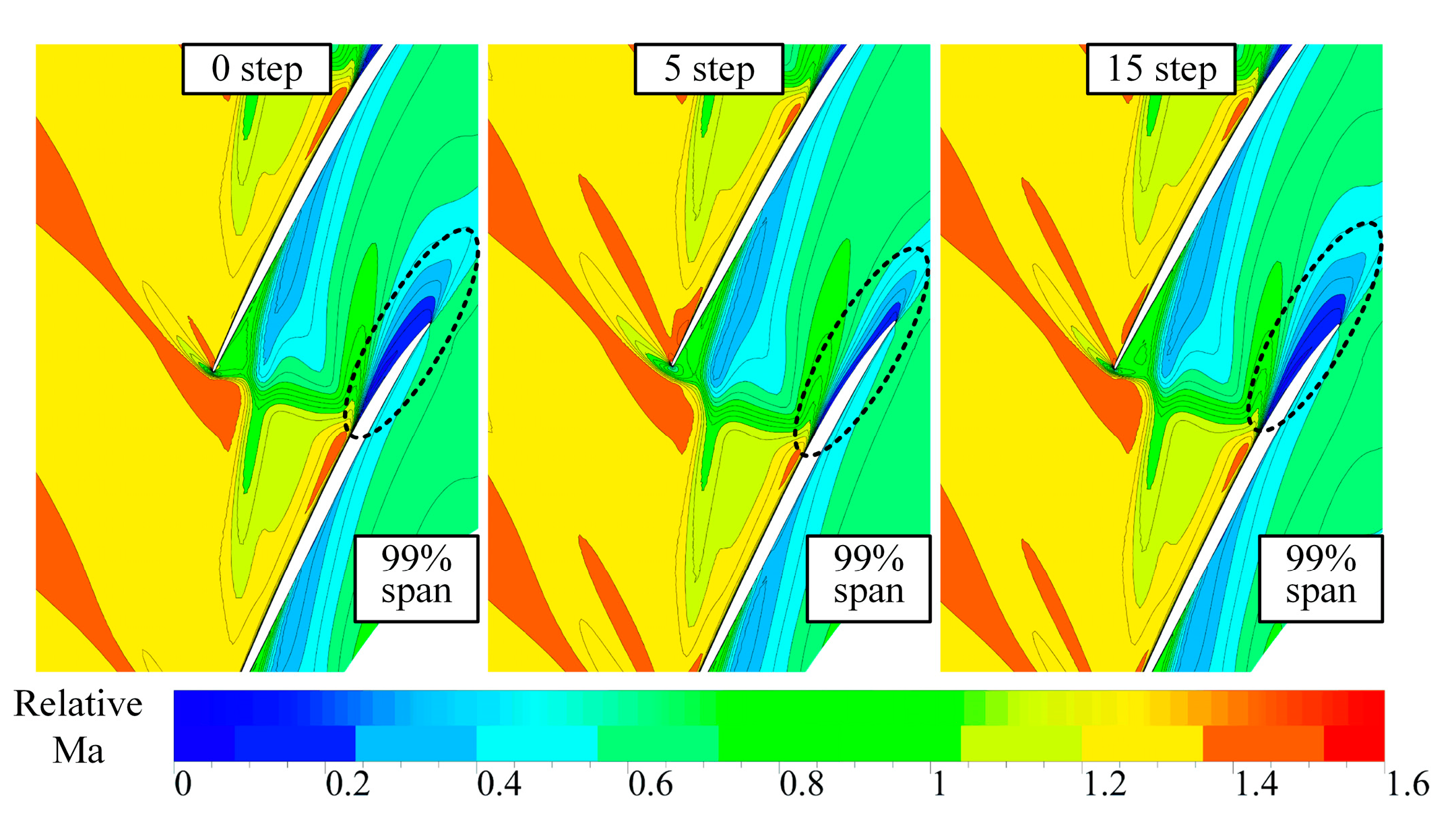
The static pressure at the 99.8% span is plotted in Figure 26. The pressure rise decreased from the front to behind the shock wave, as shown in the dashed circles in Figure 26, in which the pressure distributions are also plotted in Figure 24b. Therefore, the interaction between the TLV and the shock wave was reduced. Additionally, the initiation and development of the TLVs can be seen in the dashed ellipses. After 15 steps, the overall performance was not worse than the reference, even though the pressure rise caused by the shock wave increased slightly because the rotor generated a weaker TLV near the leading edge than after 5 steps.

The meridional velocity Vm values at 50% axial length and 80% axial length are shown in Figure 27, illustrating the flow details near the tip region. At 80% axial length, the low-energy fluid was significantly reduced after five steps. Then, after 15 steps, although the low-energy fluid partly regressed, the fluid was restricted to the tip region and mixed less with the main flow. The maximum Vm near the shroud was marked at 50% axial length surface, and the reduction in maximum Vm indicated that the TLV was reduced.

In summary, the agents improved the pressure ratio of the rotor by a combined policy that involved modifying all design variables. The additional increase in pressure was mainly produced by the change in $\mathrm{\Delta }\beta$. After the sweep and lean features were introduced and $\mathrm{\Delta }\beta$ was changed, the shock loss and separation were controlled and the loss near the tip decreased, so the efficiency of the rotor was maintained.

3.3. Off–Design Conditions

3.3.1. Near Stall

The numerical stall point was determined as the last convergence point while increasing the back pressure, as mentioned in Section 2.2. The near-stall features [50] could be identified, which verified that the near stall points were correctly found.

The axial velocity and the static pressure near the tip clearance region (99.8% span) at the last convergence point are shown in Figure 28. Negative axial velocity was observed in the dashed ellipse area, which indicates that flow spillage existed at the leading edge near tip clearance. The stagnation point moved to the pressure surface in the dashed circles. Besides this, a low-momentum area was found to be the low axial velocity area in the passage. The results confirm that the correct near-stall point was correctly found, since near-stall features appeared.

$$SM=\frac{{\dot{m}}_W}{{\dot{m}}_{stall}}\times \frac{{\pi }_{stall}}{{\pi }_W}-1$$

(15)

The stall margin was calculated with Equation (15), where ${\dot{m}}_{stall}$ and ${\pi }_{stall}$ were the mass flow rate and the pressure ratio at the last convergence point, respectively, which was considered the numerical stall point. The calculated SM of the reference rotor was $S{M}_0=6.52\%$. After 5, 10, and 15 modification steps, this value changed to $S{M}_5=7.54\%$, $S{M}_{10}=8.15\%$ and $S{M}_{15}=6.53\%$, respectively, which results are all better than the reference rotor.

3.3.2. Off-Design Speed

The operating characteristic curves were calculated at 70% of the design speed in order to consider the off-design speed performance. Figure 29 shows that the modified rotors achieved better performance than the reference rotor over the whole operating characteristic curve.

One of the mechanisms for improving the pressure ratio $\pi$ was modifying $\mathrm{\Delta }\beta$ and ${\beta }_y$, which was done by the agent and discussed in Section 3.1. This mechanism remained effective at 70% speed, so the 0.59% improvement in $\pi$ remained at the peak efficiency flow of the reference rotor.

The flow rate and the rotation speed were reduced at 70% speed, so the shock structure was weaker than that at 100% speed. After 15 modification steps, the rotor partially increased the pressure ratio using the shock wave. As a result, the efficiency was slightly reduced at 100% speed, but remained higher than that of the rotor after 10 modification steps at 70% speed.

4. Discussion

4.1. Parameter Influence on the Training Process

The hyperparameters and convergence strategy significantly influenced whether the training process was successful. Hence, the rules and experiences have been summarized for successful agent training, and different agents have been trained in the meantime.

Agents with different $r_{raw}$ values were trained with the same artificial neural network hyperparameters and different RL environment parameters, as shown in

Table 5. Parameter influence on agent convergence.

${\mathit{r}}_{\mathit{r}\mathit{a}\mathit{w}}$	Series	${\mathit{a}}_1$	${\mathit{a}}_2$	${\mathit{r}}_{\mathit{m}\mathit{i}\mathit{n}}$	${\mathit{r}}_{\mathit{m}\mathit{a}\mathit{x}}$	${\mathit{r}}_{\mathit{D}}$	$\mathit{\delta }{\mathit{r}}_{0,\mathit{a}\mathit{v}\mathit{e}}$	${\mathit{N}}_{\mathit{e}\mathit{p}}$
$\widehat{\pi }-{\widehat{\pi }}_0$	1	9.57	0.72	−0.31	0.82	1.13	−0.068	~4000
${\eta }_W-{\eta }_{W,0}$	2	27	0.90	−0.18	1.01	1.19	−0.050	~3500
$\begin{array}{l}\widehat{\eta }({\dot{m}}_h-{\dot{m}}_l)\\ -{\widehat{\eta }}_0({\dot{m}}_{h,0}-{\dot{m}}_{l,0})\end{array}$	3	38	0.90	–0.23	0.94	1.17	−0.050	~3000
	4	150	0.24	−2.91	0.95	3.86	−0.050	>14,000
$(\widehat{\eta }-{\widehat{\eta }}_0)({\dot{m}}_h-{\dot{m}}_l)$	5	500	1.00	−0.56	1.04	1.60	−0.050	~3000
$\frac{1.5}{100\left|{\dot{m}}_W-{\dot{m}}_{W,0}\right|+1}{\eta }_W$	6	1.00	0.10	−0.14	1.12	1.26	−0.050	~4000

. $N_{ep}$ is the episode when the accumulated reward was increased. $a_1$ and $a_2$ are the coefficients in the RL environment that determined $r_D$. $r_{min}$ and $r_{max}$ are the maximum and minimum rewards of 300 random sample points, respectively, and the reward range is $r_D=r_{max}-r_{min}$. $\delta r_{0,ave}$ is the average of the $\delta r_{0,i}$ values for each dimension of $p_i\in \mathbb{P}$. The ratio of $r_D$ to $\delta r_{0,ave}$ indicates how much $r_{raw}$ influenced the reward r. Two training concerns emerged from the analysis of the above training results.

First, reasonable RL environmental hyperparameters were needed. The R of the series 3 agents improved after approximately 3000 episodes, while the series 4 agents did not learn anything meaningful, even after 14,000 episodes. The difference between the series 3 and series 4 agents was $r_D$. In addition, $N_{ep}$ remained similar for different $r_{raw}$ values if $r_D$ was similar. Therefore, $r_D$ was set to be slightly larger than 1 and $\delta r_{0,ave}$ was set to −0.05, according to the training results.

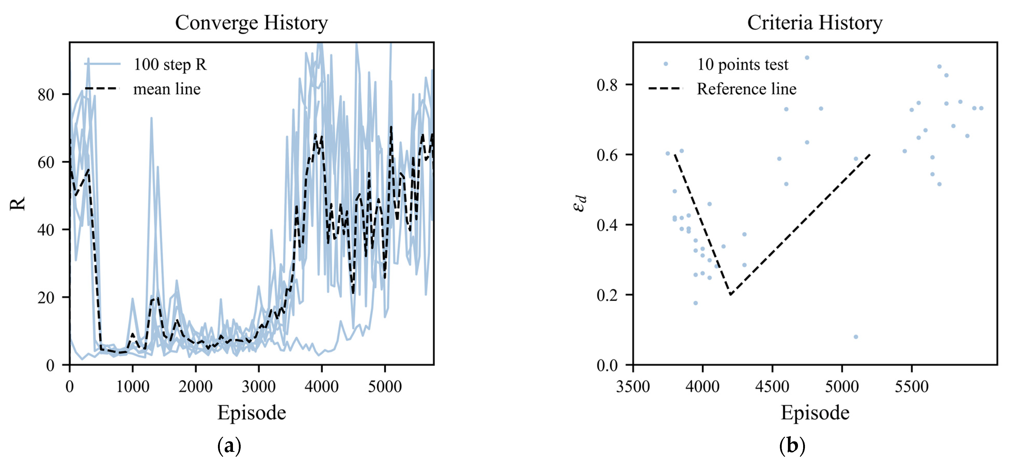
Second, the appropriate convergence strategy must be determined. Checking ${\epsilon }_d$ required relatively large amounts of calculation, so ${\epsilon }_d$ was evaluated only if the R value was higher than the threshold $R_t$. The results show that the changes in the R and ${\epsilon }_d$ were not synchronized. This phenomenon sometimes resulted in deteriorated agent performance, and was observed in different series of agents.

Figure 30 displays the R and ${\epsilon }_d$ values of 10 random testing points of the series 2 agents. The R value increased after approximately 3500 episodes, as shown in Figure 30a, then ${\epsilon }_d$ decreased firstly and then increased, as shown in Figure 30b. Therefore, the threshold for R should not be too high, or agents with acceptable R and ${\epsilon }_d$ values will be difficult to obtain. The recommended R threshold was set to 70% of the maximum.

The recommended values of parameters are summarized in

Table 6. Recommended values of parameters.

Parameter	Description	Recommended Value
$r_{max}$	Observed maximum $r_{raw}$	1.0
$r_{min}$	Observed minimum $r_{raw}$	−0.3
$\delta r_{0,ave}$	Strength of constrains	−0.05
$R_t$	Threshold of R	70
${\epsilon }_{d,t}$	Threshold of ${\epsilon }_d$	0.25

according to the analysis above. The $r_{max}$ and $r_{min}$ can be configured by calculating the $a_1$ and $a_2$ after the $r_{raw}$ is constructed. Correspondingly, the $\delta r_{0,ave}$, $R_t$, and ${\epsilon }_{d,t}$ can be adjusted directly.

The modifications to the DDPG algorithm show the advantages of reducing ${\epsilon }_d$ in rotor design environment. As shown in Figure 31, agents were trained on the original and modified DDPG algorithms, and their performances were compared. Ten agents with and without the modifications were trained using the same convergence strategy and threshold, and the best agent was selected as the final result. After the modification was applied, the ${\epsilon }_d$ value decreased from 0.136 to 0.086.

4.2. Policy for Improving the Peak Efficiency

Efficiency is another critical objective in compressor design. The series 2 agents successfully learned to improve the efficiency by setting $r_{raw}={\eta }_W-{\eta }_{W,0}$ and adjusting other parameters, where ${\eta }_{W,0}$ was the ${\eta }_W$ value of the reference rotor.

The learned policy is illustrated in Figure 32. The tip of the rotor was swept forward at the first few steps and then swept back. The negative lean feature changed to positive from the tip region to the lower span. As for 2D airfoils, the segment angle decreased mainly because of the variation in ${\chi }_{in}$.

It was mentioned in [51] that the forward and back sweep features both increased the efficiency; however, the stall margin was diminished when using the back sweep feature. The series 2 agent learned to use the back sweep feature and modified the other parameters to maintain the stall margin. Moreover, as mentioned by [43], the efficiency improved when the angle between the end wall and the suction surface was obtuse.

The operating characteristics at different step numbers are shown in Figure 33. The chock mass flow increased, and the pressure ratio remained higher than that of the reference rotor over the whole curve. The stall mass flow remained constant, showing that the penalty terms in reward worked well. The peak efficiency can be further improved by modifying more steps, shown as the 20-step case in Figure 33; however, the pressure ratio deteriorated as the number of steps increased further.

The performance at the 0.98 mass flow rate was significantly improved, with the total pressure ratio of $\pi$ = 1.643 and efficiency of $\eta$ = 0.9048 increasing to $\pi$ = 1.681 and $\eta$ = 0.9107 after 15 steps. The near-peak efficiency points are listed in

Table 7. Performance after modification by series 2 agents at different numbers of steps.

Step Number	${\dot{\mathit{m}}}_{\mathit{W}}$	${\mathit{\eta }}_{\mathit{W}}$	${\mathit{\pi }}_{\mathit{W}}$	$\mathit{\delta }{\mathit{\eta }}_{\mathit{W}}$
0	33.21	0.9088	1.679	0
5	33.74	0.9087	1.676	–0.00%
10	33.79	0.9106	1.675	0.20%
15	33.78	0.9115	1.674	0.30%
20	33.88	0.9125	1.666	0.41%

. The peak efficiency improved after the geometry was modified.

4.3. Cooperation among Different Agents

The agents learned the design policy in the whole design space; hence, the different agents could cooperate before the designers fully understood the mechanism of the policy. This universality is an exciting component of the intellectual design process.

The series 1 and 2 agents were selected for the cooperation investigation. The reference rotor was modified by series 1 agents for ten steps and series 2 agents for another ten steps. The performance of the modified rotors was assessed after different steps by the CFD method, and the operating characteristic curves are plotted in Figure 34. The pressure ratio improvement induced by the series 1 agent remained, even after modification by the series 2 agent. Moreover, the peak efficiency improved rather than decreasing after 15 steps, as observed in Figure 17.

The cooperation policy performed better than single policies. After 20 steps in the cooperated modification process, the new rotor showed a higher $\eta$ than the series 1 agent result (see Table 4), and a higher $\pi$ than the series 2 agent results (see Table 7), with $\pi$ = 1.678 and $\eta$ = 0.9111 at the near-peak efficiency point. The 0.98 mass flow rate performance was $\pi$ = 1.683 and $\eta$ = 0.9105, which results are in between the performance of the two single agent results.

5. Conclusions

This study constructed a reinforcement learning framework using the modified DDPG algorithm to learn the design policies of transonic rotors. The RL agents learned similarly to humans and generated policies to improve the pressure ratio and efficiency, while maintaining the other performances. The flow field analyses of the improved rotors demonstrated the effectiveness of the learned policy. The cooperation of different agents showed an advantage over using the agents alone. Additionally, different agents were trained, and the rules have been summed up to guide further training. If the case is changed, most of the variables that need tuning have candidate values or have an objective to meet, which benefits the general applicability.

The modifications made the DDPG algorithm fit the usage of aerodynamic design better. The high-order feedback, virtual area, and artificial tip accelerated the training process. The presented error reduction process significantly improved the performance of the kriging models and reduced the number of required sample points. The trained agent modified the geometric parameters to improve the pressure ratio and reduce the loss in the tip region by changing $\mathrm{\Delta }\beta$ and introducing sweep and lean features. As a result, the pressure ratio of the modified rotor improved by 1.01% with the same efficiency and flow rate, and can be further improved. Additionally, this work considered the cooperation of different agents, and found that this improved the $\pi$ and $\eta$.

In summary, the present study is one of the first attempts to apply RL methods in 3D compressor design. RL methods are universal and more flexible than algorithms that find optimized points. Since the cooperation of agents has shown an advantage, a natural progression of this work is to integrate more prior knowledge and other design methods into the RL framework. The follow-up research could also explore the application of RL methods in more expansive design spaces and multistage cases after the improvements are incorporated.

The engine manufacturers possess plenty of simulation and experimental data, which may help to realize more potential abilities of RL methods. The trained agents can assist designers before they fully understand the fluid mechanism by improving factors such as pressure ratio and efficiency, or moving the working point, thus accelerating the iteration of products. Once agents’ abilities are improved further, they may outperform humans, and generate compressor designs automatically, thus outperforming humans in other fields.

References

1. Ning, X.; Lovell, M.R. On the sliding friction characteristics of unidirectional continuous FRP composites. J. Tribol. 2002, 124, 5–13. [Google Scholar] [CrossRef]
2. Steffens, K. Advanced compressor technology—Key success factor for competitiveness in modern aero engines. In Proceedings of the 15th International Symposium on Air Breathing Engines (ISABE), Bangalore, India, 2–7 September 2001. [Google Scholar]
3. Biollo, R.; Benini, E. Recent advances in transonic axial compressor aerodynamics. Prog. Aerosp. Sci. 2013, 56, 1–18. [Google Scholar] [CrossRef]
4. Smith, L.H. Axial compressor aerodesign evolution at general electric. J. Turbomach. 2002, 124, 321–330. [Google Scholar] [CrossRef]
5. Horlock, J.H.; Denton, J.D. A review of some early design practice using computational fluid dynamics and a current perspective. J. Turbomach. 2005, 127, 5–13. [Google Scholar] [CrossRef]
6. Pinto, R.N.; Afzal, A.; D’Souza, L.V.; Ansari, Z.; Samee, A.D.M. Computational fluid dynamics in turbomachinery: A review of state of the art. Arch. Comput. Methods Eng. 2016, 24, 467–479. [Google Scholar] [CrossRef]
7. Dunham, J. CFD Validation for Propulsion System Components; AGARD: Gatineau, QC, Canada, 1998. [Google Scholar]
8. Jennions, I.K.; Turner, M.G. Three–dimensional navier—Stokes computations of transonic fan flow using an explicit flow solver and an implicit κ–ε solver. J. Turbomach. 1993, 115, 261–272. [Google Scholar] [CrossRef]
9. Samad, A. Turbomachinery Design; LAP LAMBERT Academic Publishing GmbH & Co.KG: Saarbrucken, Germany, 2012. [Google Scholar]
10. Kim, K.–Y.; Samad, A.; Benini, E. Design Optimization of Fluid Machinery: Applying Computational Fluid Dynamics and Numerical Optimization; John Wiley & Sons, Incorporated: Newark, NJ, USA, 2019. [Google Scholar]
11. Li, Z.; Zheng, X. Review of design optimization methods for turbomachinery aerodynamics. Prog. Aerosp. Sci. 2017, 93, 1–23. [Google Scholar] [CrossRef]
12. Bonaiuti, D.; Zangeneh, M. On the coupling of inverse design and optimization techniques for the multiobjective, multipoint design of turbomachinery blades. J. Turbomach. 2009, 131, 21014–21019. [Google Scholar] [CrossRef]
13. Deb, K.; Pratap, A.; Agarwal, S.; Meyarivan, T. A fast and elitist multiobjective genetic algorithm: NSGA–II. IEEE Trans. Evol. Comput. 2002, 6, 182–197. [Google Scholar] [CrossRef]
14. Ma, S. –B.; Roh, M.–S.; Kim, K.–Y. Optimization of discrete cavities with guide vanes in a centrifugal compressor based on a comparative analysis of optimization techniques. Int. J. Aeronaut. Space Sci. 2021, 22, 514–530. [Google Scholar] [CrossRef]
15. Eberhart, R.; Kennedy, J. A new optimizer using particle swarm theory. In Proceedings of the Sixth International Symposium on Micro Machine and Human Science—MHS’95, Nagoya, Japan, 4–6 October 1995. [Google Scholar]
16. Mirjalili, S.; Lewis, A. The whale optimization algorithm. Adv. Eng. Softw. 2016, 95, 51–67. [Google Scholar] [CrossRef]
17. Huang, S.; Yang, C.; Han, G.; Zhao, S.; Lu, X. Multipoint design optimization for a controlled diffusion airfoil compressor cascade. Proc. Inst. Mech. Eng. C J. Mech. Eng. Sci. 2020, 234, 2143–2159. [Google Scholar] [CrossRef]
18. Tang, X.; Luo, J.; Liu, F. Aerodynamic shape optimization of a transonic fan by an adjoint–response surface method. Aerosp. Sci. Technol. 2017, 68, 26–36. [Google Scholar] [CrossRef]
19. Strazisar, A.J.; Wood, J.R.; Hathaway, M.D.; Suder, K.L. Laser Anemometer Measurements in a Transonic Axial—Flow Fan Rotor; NASA: Cleveland, OH, USA, 1989. [Google Scholar]
20. Du, Q.; Yang, L.; Li, L.; Liu, T.; Zhang, D.; Xie, Y. Aerodynamic design and optimization of blade end wall profile of turbomachinery based on series convolutional neural network. Energy 2022, 244, 122617. [Google Scholar] [CrossRef]
21. Sutton, R.S.; Barto, A.G. Reinforcement Learning: An Introduction, 2nd ed.; The MIT Press: Cambridge, MA, USA; London, UK, 2020. [Google Scholar]
22. Tan, R.K.; Liu, Y.; Xie, L. Reinforcement learning for systems pharmacology–oriented and personalized drug design. Expert Opin. Drug Discov. 2022, 17, 849–863. [Google Scholar] [CrossRef]
23. Senior, A.W.; Evans, R.; Jumper, J.; Kirkpatrick, J.; Sifre, L.; Green, T.; Qin, C.; Žídek, A.; Nelson, A.W.R.; Bridgland, A.; et al. Improved protein structure prediction using potentials from deep learning. Nature 2020, 577, 706–710. [Google Scholar] [CrossRef] [PubMed]
24. Fawzi, A.; Balog, M.; Huang, A.; Hubert, T.; Romera–Paredes, B.; Barekatain, M.; Novikov, A.; Ruiz, F.J.R.; Schrittwieser, J.; Swirszcz, G.; et al. Discovering faster matrix multiplication algorithms with reinforcement learning. Nature 2022, 610, 47–53. [Google Scholar] [CrossRef] [PubMed]
25. Sigaud, O.; Stulp, F. Policy search in continuous action domains: An overview. Neural Netw. 2019, 113, 28–40. [Google Scholar] [CrossRef] [PubMed]
26. Viquerat, J.; Rabault, J.; Kuhnle, A.; Ghraieb, H.; Larcher, A.; Hachem, E. Direct shape optimization through deep reinforcement learning. J. Comput. Phys. 2021, 428, 110080. [Google Scholar] [CrossRef]
27. Schulman, J.; Wolski, F.; Dhariwal, P.; Radford, A.; Klimov, O. Proximal policy optimization algorithms. arXiv 2017, arXiv:1707.06347. [Google Scholar] [CrossRef]
28. Li, R.; Zhang, Y.; Chen, H. Learning the aerodynamic design of supercritical airfoils through deep reinforcement learning. AIAA J. 2021, 59, 3988–4001. [Google Scholar] [CrossRef]
29. Qin, S.; Wang, S.; Wang, L.; Wang, C.; Sun, G.; Zhong, Y. Multi–objective optimization of cascade blade profile based on reinforcement learning. Appl. Sci. 2020, 11, 106. [Google Scholar] [CrossRef]
30. Lillicrap, T.P.; Jonathan, J.H.; Pritzel, A.; Heess, N.; Erez, T.; Tassa, Y.; Silver, D.; Wierstra, D. Continuous control with deep reinforcement learning. arXiv 2016, arXiv:1509.02971. [Google Scholar] [CrossRef]
31. Li, J.; Zhang, M.; Martins, J.R.R.A.; Shu, C. Efficient aerodynamic shape optimization with deep–learning–based geometric filtering. AIAA J. 2020, 58, 4243–4259. [Google Scholar] [CrossRef]
32. Hammond, J.; Pepper, N.; Montomoli, F.; Michelassi, V. Machine learning methods in CFD for turbomachinery: A review. Int. J. Turbomach. Propuls. Power 2022, 7, 16. [Google Scholar] [CrossRef]
33. Hammond, J.; Pietropaoli, M.; Michelassi, V.; Sandberg, R.D.; Montomoli, F. Machine learning for the development of data–driven turbulence closures in coolant systems. J. Turbomach. 2022, 144, 081003. [Google Scholar] [CrossRef]
34. Wang, Z.Y.; Qu, F.; Wang, Y.H.; Luan, Y.G.; Wang, M. Research on the lean and swept optimization of a single stage axial compressor. Eng. Appl. Comput. Fluid Mech. 2021, 15, 142–163. [Google Scholar] [CrossRef]
35. Duan, Y.; Zheng, Q.; Jiang, B.; Lin, A.; Zhao, W. Implementation of Three-Dimensional Inverse Design and Its Application to Improve the Compressor Performance. Energies 2020, 13, 5378. [Google Scholar] [CrossRef]
36. Ren, X.; Gu, C. Investigation of Compressor Tip Clearance Flow Based on the Discontinuous Galerkin Methods. In Proceedings of the ASME Turbo Expo 2013: Turbine Technical Conference and Exposition, San Antonio, TX, USA, 3–7 June 2013. [Google Scholar] [CrossRef]
37. Jung, Y. –J.; Jeon, H.; Jung, Y.; Lee, K.–J.; Choi, M. Effects of recessed blade tips on stall margin in a transonic axial compressor. Aerosp. Sci. Technol. 2016, 54, 41–48. [Google Scholar] [CrossRef]
38. Chen, H.; Huang, X.; Fu, S. CFD Investigation on stall mechanisms and casing treatment of a transonic compressor. In Proceedings of the 42nd AIAA/ASME/SAE/ASEE Joint Propulsion Conference & Exhibit, American Institute of Aeronautics and Astronautics: Sacramento, CA, USA, 9–12 July 2006. [Google Scholar]
39. Kingma, D.P.; Ba, J. Adam: A method for stochastic optimization. arXiv 2015, arXiv:1412.6980. [Google Scholar]
40. Qie, H.; Shi, D.; Shen, T.; Xu, X.; Li, Y.; Wang, L. Joint optimization of multi–UAV target assignment and path planning based on multi—Agent reinforcement learning. IEEE Access 2019, 7, 146264–146272. [Google Scholar] [CrossRef]
41. Forrester, A.I.J. Engineering Design via Surrogate Modelling: A Practical Guide; Wiley: Chichester, UK, 2008. [Google Scholar]
42. Morris, M.D.; Mitchell, T.J. Exploratory designs for computational experiments. J. Stat. Plan. Inference 1995, 43, 381–402. [Google Scholar] [CrossRef]
43. Zheng, X.; Li, Z. Blade—End treatment to improve the performance of axial compressors: An overview. Prog. Aerosp. Sci. 2017, 88, 1–14. [Google Scholar] [CrossRef]
44. Denton, J.D. The Effects of Lean And Sweep on Transonic Fan Performance: A Computational Study. In Proceedings of the ASME Turbo Expo 2002: Power for Land, Sea, and Air, Amsterdam, The Netherlands, 3–6 June 2002. [Google Scholar] [CrossRef]
45. Denton, J.D.; Xu, L. The exploitation of three–dimensional flow in turbomachinery design. Proc. Inst. Mech. Eng. C J. Mech. Eng. Sci. 1998, 213, 125–137. [Google Scholar] [CrossRef]
46. Sasaki, T.; Breugelmans, F. Comparison of sweep and dihedral effects on compressor cascade performance. J. Turbomach. 1998, 120, 454–463. [Google Scholar] [CrossRef]
47. Shang, E.; Wang, Z.Q.; Su, J.X. The experimental investigations on the compressor cascades with leaned and curved blade. In Proceedings of Volume 1: Aircraft Engine; Marine; Turbomachinery; Microturbines and Small Turbomachinery; American Society of Mechanical Engineers: Cincinnati, OH, USA, 1993; p. V001T003A018. [Google Scholar]
48. Chima, R.V. Calculation of tip clearance effects in a transonic compressor rotor. J. Turbomach. 1998, 120, 131–140. [Google Scholar] [CrossRef]
49. Suder, K.L.; Celestina, M.L. Experimental and computational investigation of the tip clearance flow in a transonic axial compressor rotor. J. Turbomach. 1996, 118, 218–229. [Google Scholar] [CrossRef]
50. Hah, C.; Bergner, J.; Schiffer, H.–P. Short length–scale rotating stall inception in a transonic axial compressor: Criteria and mechanisms. In Proceedings of Volume 6: Turbomachinery, Parts A and B; ASMEDC: Barcelona, Spain, 2006; pp. 61–70. [Google Scholar]
51. Neshat, M.A.; Akhlaghi, M.; Fathi, A.; Khaledi, H. Investigating the effect of blade sweep and lean in one stage of an industrial gas turbine’s transonic compressor. Propuls. Power Res. 2015, 4, 221–229. [Google Scholar] [CrossRef] [Green Version]
Figure 1. Overall structure of the intellectual design framework, which had a hierarchical structure. The CFD manager calculated the operating characteristics of the rotors in multiple threads, determined the performance and managed the data.
Aerospace 10 00171 g001
Figure 2. Comparison of the original and generated rotor on the z r a and m θ r a surfaces. The directions of the sweep and lean are marked.
Aerospace 10 00171 g002
Figure 3. Definition of the camber angles and incidence.
Aerospace 10 00171 g003
Figure 4. Grid of the rotor with 1.2 M nodes and O–H topology.
Aerospace 10 00171 g004
Figure 5. Operating characteristic of NASA rotor 67, with 0.8 M, 1.2 M and 1.6 M grids. (a) The total pressure ratio curve. (b) The efficiency curve.
Aerospace 10 00171 g005
Figure 6. Variable distributions in the span in the experiment [19] and CFD simulations: (a) pressure distribution in the span; (b) temperature distribution in the span.
Aerospace 10 00171 g006
Figure 7. Typical operating characteristic curve according to the CFD calculations, including the definitions of 7 selected performance variables.
Aerospace 10 00171 g007
Figure 8. Distortion at the end of the process with a random initial state. The processes in high-dimensional design space were projected onto a dimensionless β ^ y , 2 χ ^ i n , 2 surface. (a) Agent with mild distortion. (b) Agent with severe distortion.
Aerospace 10 00171 g008
Figure 9. High-order feedback does not directly affect the influencing interactions between the agent and the environment.
Aerospace 10 00171 g009
Figure 10. Virtual area and penalty term; δ r v i r is zero when the state is in the real design space.
Aerospace 10 00171 g010
Figure 11. Processes generated by normal and abnormal agents.
Aerospace 10 00171 g011
Figure 12. Training agents in the demo case. The average point and minimum ε d value of each version were compared.
Aerospace 10 00171 g012
Figure 13. Schematic of the error reduction process. The overall performance of the model improved after restricting the points with poor performance.
Aerospace 10 00171 g013
Figure 14. R 2 of π W and η ^ with and without error reduction training for different numbers of sample points. (a) R 2 of π W . (b) R 2 of η ^ .
Aerospace 10 00171 g014
Figure 15. Surrogate models with 7 (i = 1, 2, …, 7) selected performance variables trained in various configurations with different numbers of sample points N.
Aerospace 10 00171 g015
Figure 16. Modification of the design variables at different step numbers.
Aerospace 10 00171 g016
Figure 17. Variation in the rotor operating characteristic curves after different steps for the series 1 agent. (a) Flow–pressure ratio. (b) Flow–efficiency.
Aerospace 10 00171 g017
Figure 18. Variations in the geometric parameter distributions in the spanwise direction after modification by series 1 agents: (a) meridional coordinate; (b) tangential direction; (c) inlet camber angle; (d) outlet camber angle; (e) incidence angle.
Aerospace 10 00171 g018
Figure 19. Different geometries modified by the agents.
Aerospace 10 00171 g019
Figure 20. The deviations of the local performance distributions in different spans: (a) pressure ratio; (b) efficiency; (c) absolute flow angle.
Aerospace 10 00171 g020
Figure 21. Isentropic Mach number distribution through the chord line at 70% and 90% span. (a) 70% span. (b) 90% span.
Aerospace 10 00171 g021
Figure 22. Separation in the near-tip span region.
Aerospace 10 00171 g022
Figure 23. The static pressure distributions in the near-tip region.
Aerospace 10 00171 g023
Figure 24. Static pressure distributions through the chord line near and around the tip span. (a) 90% span. (b) 99.8% span.
Aerospace 10 00171 g024
Figure 25. Axial velocity distributions at the tip clearance span (99.8%).
Aerospace 10 00171 g025
Figure 26. Static pressure distributions in the tip clearance span region (99.8%).
Aerospace 10 00171 g026
Figure 27. Meridional velocity at 50% and 80% axial length.
Aerospace 10 00171 g027
Figure 28. The near-stall flow details; Vz and statistical pressure are plotted at the tip clearance span (99.8%).
Aerospace 10 00171 g028
Figure 29. Operation characteristic curves at 70% design speed. (a) Flow pressure ratio. (b) Flow efficiency.
Aerospace 10 00171 g029
Figure 30. Changes in R and ε d when training series 2 agents. (a) Converge history of series 2. (b) Criteria history of series 2.
Aerospace 10 00171 g030
Figure 31. The improvement with the modified algorithm.
Aerospace 10 00171 g031
Figure 32. Variations of the geometric parameter distributions in the spanwise direction after modification by series 2 agents: (a) meridional coordinate; (b) tangential direction; (c) inlet camber angle; (d) outlet camber angle; (e) incidence angle.
Aerospace 10 00171 g032
Figure 33. Variation in the operating characteristic curves of rotors after different numbers of steps after modification by series 2 agents. (a) Flow pressure ratio. (b) Flow efficiency.
Aerospace 10 00171 g033
Figure 34. Variation in the operating characteristic curves of the rotors after cooperation between series 1 and series 2 agents. (a) Flow pressure ratio. (b) Flow efficiency.
Aerospace 10 00171 g034