Article

Surrogate Aerodynamic Wing Modeling Based on a Multilayer Perceptron

by
Oscar Ulises Espinosa Barcenas
1,*,
Jose Gabriel Quijada Pioquinto
1,
Ekaterina Kurkina
2 and
Oleg Lukyanov
1
1
Department of Aircraft Construction and Design, Samara National Research University, 34 Moskovskoe Shosse, Samara 443086, Russia
2
Department of Further Mathematics, Samara National Research University, 34 Moskovskoe Shosse, Samara 443086, Russia
*
Author to whom correspondence should be addressed.
Aerospace 2023, 10(2), 149; https://doi.org/10.3390/aerospace10020149
Submission received: 20 December 2022 / Revised: 3 February 2023 / Accepted: 3 February 2023 / Published: 6 February 2023
(This article belongs to the Section Aeronautics)

Abstract

:
The aircraft conceptual design step requires a substantial number of aerodynamic configuration evaluations. Since the wing is the main aircraft lifting element, the focus is on solving direct and reverse design problems. The former could be solved using a low-cost computational model, but the latter is unlikely, even for these models. Surrogate modeling is a technique for simplifying complex models that reduces computational time. In this work, a surrogate aerodynamic model, based on the implementation of a multilayer perceptron (MLP), is presented. The input data consist of geometrical characteristics of the wing and airfoil and flight conditions. Some of the MLP hyperparameters are defined using evolutionary algorithms, learning curves, and cross-validation methods. The MLP predicts the aerodynamic coefficients (drag, lift, and pitching moment) with high agreement with the substituted aerodynamic model. The MLP can predict the aerodynamic characteristics of compressible flow up to 0.6 M. The developed MLP has achieved up to almost 800 times faster in computing time than the model on which it was trained. The application of the developed MLP will enable the rapid study of the effects of changes in various parameters and flight conditions on flight performance, related to the design and modernization of new vehicles.

1. Introduction

Aircraft conceptual design is crucial and often relies on the designer’s intuition and experience. Works by Jager [1], Roskam [2], and Torenbeek [3] introduced a more deterministic process, focusing on individual disciplines and quick decision making. Among these disciplines, aerodynamics plays a significant role in determining aircraft layout and configuration, and thus receives special attention. Aerodynamic design has evolved over time, starting with experimentation and simple calculations [4], but advancing with more computer power and precise numerical computation [4]. Recent advancements in computational fluid dynamics have focused on improving turbulent models for aerodynamic calculations. However, despite the increased accuracy, the complexity of these mathematical models can make it more difficult to evaluate multiple aerodynamic configurations during the conceptual design stage.
Current design methodologies in aerodynamic design involve multidisciplinary analysis and optimization [4,5], robust design [4,6,7], and surrogate modeling [4,8]. Surrogate modeling is a technique that can be used to approximate the behavior of a complex system and is an efficient alternative to multidisciplinary analysis and optimization (MDAO) and robust design. It offers several advantages such as speed, efficiency, flexibility, ease of interpretation, robustness, and the ability to handle high-dimensional problems. Surrogate models can be used to quickly identify optimal solutions and can provide insights into the relationships between design variables and performance metrics. Additionally, they are less sensitive to noise and uncertainty and can be used to generate accurate predictions, even with incomplete data. Artificial intelligence, especially machine learning, had demonstrated that it could be potentially applied in aerodynamic design as a surrogate method. For instance, neural networks for predicting the aerodynamic coefficients of airfoils [9,10] and wings [10], or airfoil inverse design [11,12], have been developed and demonstrated to speed up the design process, with the added advantage of predicting solutions to nonlinear problems efficiently and accurately [9].
Neural networks aimed at modeling aerodynamic data have two main approaches: aerodynamic response prediction and reconstruction of flow fields. Aerodynamic response predictions refer to the use of appropriate methods to build aerodynamic data models that can express the variation in aerodynamic response parameters (force or moment coefficients) with the design parameters and output the predicted value of the response parameters in the case of given design parameters. This type of network can be used in both direct and inverse design processes [13]. Studies in this field typically focus on two aspects: those that are based on the flow state when only numerical flow data are provided, and those that consider both aerodynamic shapes and the flow state when graphic information of the flow and bodies immersed in the flow is also available. When making steady aerodynamic response predictions, both multilayer perceptron (MLP) neural networks and convolutional neural networks (CNN) can be used. The choice of MLP and CNN depends on the task at hand and the available data. In this work, the information that determines the wing configuration and flow conditions is presented in vector form, and the goal is to predict the values of the aerodynamic coefficients. In this case, an MLP architecture is better suited to this task.
Throughout history, several MLPs have been developed for predicting aerodynamic coefficients, from predicting a single coefficient for an airfoil [11,14] to predicting multiple coefficients for an airfoil [9,15,16], to predicting aerodynamic coefficients of wing configurations [17]. One of the most developed architectures for predicting aerodynamic coefficients of wing configurations is the one developed by Secco and Mattos. They developed a methodology for creating an MLP capable of predicting either the lift coefficient or the drag coefficient. To accomplish this, they required 40 input parameters, which described the complex wing geometry (including a kink station) and flow characteristics.
The development of new MLP architectures for improving prediction accuracy requires considering model-oriented research [18]. One approach for achieving this is to perform hyperparameter tuning of the MLP using optimization methods such as evolutionary and genetic algorithms [9,15,16,19]. These algorithms have been shown to be efficient in determining optimal hyperparameters compared to traditional methods such as grid search [19]. Additionally, they are simple to implement and can adapt to integer encoding, which is necessary for obtaining the number of neurons per layer [20]. Regardless of the optimization algorithm chosen, it is important to evaluate the performance of each architecture by varying the hyperparameters. One widely used method for determining the appropriate values of the performance metrics is cross-validation. Cross-validation is a statistical method used to estimate the performance of deep learning models, and it helps to prevent overfitting in cases where data may be limited [19,21].
The objective of this study was to reduce the computation time in aerodynamic wing conceptual design by replacing an aerodynamic mathematical model (AMM) based on the vortex lattice method and empirical equations with a MLP. An alternative methodology, compared to the one presented by Secco and Mattos, is presented to develop an MLP, which includes novel features such as hyperparameter tuning using an evolutionary algorithm and the use of the cross-validation method to evaluate the performance of the trained networks. Additionally, the proposed MLP is able to predict drag, lift, and pitching moment coefficients of wing configurations simultaneously, which marks the novelty of the present work. Furthermore, the presented MLP can predict the aerodynamic coefficients of a wing in steady compressible viscid flow with high accuracy, and requires a minimal amount of computational and time costs compared to using numerical modeling methods of aerodynamics based on the solution of Navier–Stokes equations. The utility of the developed MLP in constructing a surrogate aerodynamics model for aerodynamic design not only reduces computation time but also allows for the parallel computation of multiple wing configurations, with great agreement with the values given by the replaced AMM. The academic value relies on the application of the developed MLP for a rapid study of the effects of changes in various parameters and flight conditions on flight performance, related to the design and modernization of new vehicles.
This work is structured as follows: Section 2 describes the necessary parameters to describe the wing geometry and the physical characteristics of the flow, the mathematical model used to obtain the aerodynamic coefficients, the methodology for obtaining the hyperparameters of the MLP, and MLP training and performance evaluation techniques; Section 3 presents the results and discussions obtained; and finally, Section 4 presents the conclusions.

2. Materials and Methods

2.1. Design Space and Output Data Determination

2.1.1. Design Variables

The aerodynamic coefficients depend on both the geometric characteristics and flight conditions. The geometric characteristics can be divided into those of the airfoil and wing. The Bezier–PARSEC parameterization method [22], using the BP3333 variant, was chosen to perform the geometric modeling of the airfoils (as shown in Figure 1). The BP3333 variant requires the use of four third-order Bezier curves; two of these curves represent the camber line (leading edge and trailing edge), and the other two represent the shape of the airfoil thickness (leading edge and trailing edge). Each curve is constructed using the parametric Equations (1) and (2).
x(u) = x0(1 − u)3 + 3x1u(1 − u)2 + 3x2u2(1 − u) + x3u3,
y(u) = y0(1 − u)3 + 3y1u(1 − u)2 + 3y2u2(1 − u) + y3u3,
where u is the parameter that ranges from 0 to 1; xi, yi are the coordinates of the Bezier control points.
The Bezier control points are determined in terms of 12 PARSEC parameters, which represent the following aerodynamic characteristics of the airfoil: rle is the leading-edge radius, αte is the trailing camber line angle, βte is the trailing-edge angle, zte is the trailing-edge vertical displacement, γle is the leading-edge direction, (xc, yc) is the location of the maximum camber, kc is the curvature of the maximum camber, (xt, yt) is the position of the maximum thickness, kt is the curvature of the maximum thickness, and dzte is the half-thickness of the trailing edge. The Bezier control points [22] for the leading-edge thickness curve are calculated using the following expressions:
{ x 0 t = 0 x 1 t = 0 x 2 t = b 9 x 3 t = x t { y 0 t = 0   y 1 t = 3 2 k t ( x t b 9 ) 2 + y t y 2 t = y t y 3 t = y 1
The control points of the trailing-edge thickness curve are calculated with Equation (4):
{ x 0 t = x t x 1 t = 2 x t b 9 x 2 t = 1 + [ dz te ( 3 2 k t ( x t b 9 ) 2 + y t ) ] cot ( β te ) x 3 t = 1 { y 0 t = y t y 1 t = y t y 2 t = 3 2 k t ( x t b 9 ) 2 + y t y 3 t = d z te
where b9 is a Bezier parameter that can be computed by solving the next equation:
27/4kt2b94 – 27ktxtb93 + (9ktyt + 81/2kt2xt2)b92 + (2rle – 18kt2xtyt – 27kt2xt3)b9 + (3yt2 + 9ktxt2yt + 27/4kt2xt4) = 0,
and must meet the condition max{0, xt − (−2yt/3kt)1/2} < b9 < xt.
The Bezier control points for the leading-edge camber curve are calculated with the following equation:
{ x 0 1 = 0 x 0 1 = b 1 cot ( γ le ) x 2 1 = x c 2 ( b 1 y c ) 3 k c x 3 1 = x c { y 0 1 = 0   y 1 1 = b 1 y 2 1 = y c y 3 1 = y c
and the Bezier control points for the trailing-edge camber curve are calculated as:
{ x 0 2 = x c x 1 2 = x c + 2 ( b 1 y c ) 3 k c x 2 2 = 1 + ( z te b 1 ) cot ( α te ) x 3 2 = 1 { y 0 2 = y c   y 1 2 = y c y 2 2 = b 1 y 3 2 = z te
where b1 is a Bezier parameter, which is calculated from the next equation:
b1(cotγle + cotαte) + 8((b1 – yc)/6kc)1/2 – ztecotαte −1 = 0,
and must meet the condition 0 ≤ b1 ≤ yc.
The BP3333 parameterization method has demonstrated good performance when used in metaheuristic models, mainly due to the small number of parameters required. However, one of the main disadvantages of this method is the small number of degrees of freedom, particularly at the trailing edge of the airfoil [16,22]. The wing was modeled using six parameters: the aspect ratio AR, leading-edge sweep angle ΛLE, taper ratio λ, geometric twist τ, dihedral angle Γ, and wing area S. The flight conditions were represented by two parameters: the flight speed v and the angle of attack α.

2.1.2. Aerodynamic Coefficient Calculation

The calculation of the aerodynamic coefficients was performed using Athena Vortex Lattice [23], a numerical method based on the vortex lattice method (VLM), for calculating the lift CL, inductive drag CDi, and pitch moment coefficients CM, as well as empirical formulas for calculating the parasitic drag CD0. The total drag was calculated as the sum of the parasitic and inductive drag, i.e., CD = CDi + CD0.
The VLM uses the Biot–Savart–Laplace law, which states that the velocity at a point due to a vortex is proportional to the strength of the vortex and the distance from the vortex. By calculating the strengths and positions of the vortices, the VLM can determine the velocity and pressure distribution around the aircraft, which can then be used to calculate the lift, drag, and pitch moment coefficients. The lift, inductive drag, and pitch moment coefficients are given by the formulas: CL = L/QS, CDi = Di/QS, CM = M/QSc, respectively, where L is the lift; Di is the inductive drag; M is the moment; S is the wing area; Q = 0.5ρV2 is the dynamic pressure, where ρ is the air density, and V is the free-flow velocity; and c is the mean aerodynamic chord length.
The following empirical formulas were used for calculating the parasitic drag CD0:
CD0 = 2Cf ηc ηM,
Cf = 0.087 (1 − xK)/(logRe – 1.6)2 + 1.33 (xK)1/2/(Re)1/2,
ηc = 1 + 2t e−2.4xK + 9t e−4xK,
ηM = (1/(1 + 0.2M2)1/2 + 0.055xK2 M)(1 + 5t M),
xK = xK0 ky kM,
xK0 = t xt/(t + 0.02) + 0.95/(10−6Re + 2.4),
kχ = (1 – 0.6sin2ΛLE) cos2ΛLE,
kM = 1 + 0.35(M)1/2
where Cf is the friction coefficient of one side of a flat plate in an incompressible flow, ηc is the pressure resistance contribution, ηM is the compressibility effect contribution, M is the Mach number, Re is the Reynolds number, xK is the transition point position, and t = 2yt is the relative profile thickness [24]. The lift and induced drag coefficient account for the compressibility effects by applying the Prandtl–Glauert transformation, which is described as follows: CLPG = CL/β and CDiPG = CDi/β, respectively, where β = (1 − M)0.5.
The inductive drag coefficient was computed in the far field, i.e., on the Trefftz plane. It was assumed that the aerodynamic calculation was performed in a standard atmospheric pressure at sea level. The pitching moment coefficient was calculated with respect to the leading edge of the mean aerodynamic chord. The calculation of the lift and induced drag coefficient was performed on a mesh consisting of 300 panels, 30 vortices with a cosine distribution along the chordwise, and 10 vortices with a sine distribution along the semispanwise. This mesh configuration was previously verified in the work [25] by performing a mesh independence analysis. The errors for the lift, inductive drag, and pitching moment coefficients were 0.97%, 0%, and 0.88%, respectively [25].

2.2. Verification of the Aerodynamic Mathematical Model

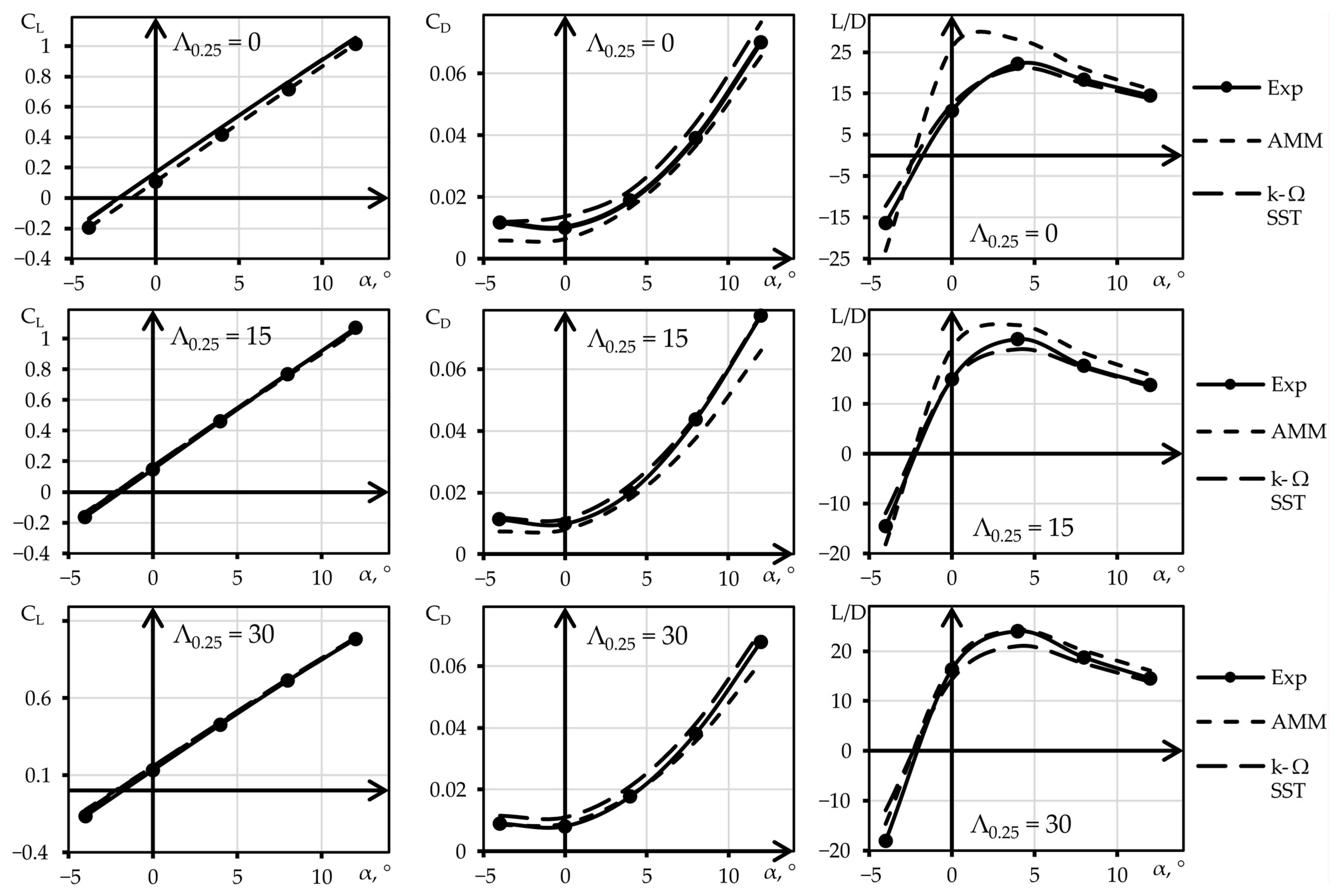
Three wings with different sweep angles were analyzed to validate the mathematical model used for generating the database. For all the wings, the aspect ratio was 6 and the taper ratio was 0.5. The airfoil used for the analysis was the NACA 24XX, and the thickness value for calculating the parasitic drag corresponded to the thickness of the mean aerodynamic chord, which was calculated from the dimensions of the real wing (with a thickness of 15% at the root section and 9% at the tip section). The free-flow velocity was 21.30 m/s. The wing was scaled geometrically to match the Reynolds number of the experiment, been 3.09 × 10⁶.
The experimental data for these wings can be found in the work [26]. It is important to note that this experiment was performed in a highly pressurized wing tunnel, specifically at 20 atmospheres. Furthermore, analysis using the turbulent model k-Ω SST was performed with the objective of demonstrating the performance of this high-accuracy model as well as comparing the computing time of both models.
The lift and drag curves as well as the lift-to-drag ratio are presented in Figure 2. The results of the verification demonstrate that the mathematical model used predicts the lift and drag coefficient values with enough accuracy. The mean absolute errors (MAE) for the lift coefficient, drag coefficient, and lift-to-drag-ratio are presented in Table 1. Moreover, the computation time of the AMM was 0.141 CPU-s, while that of the k-Ω SST was 3709.12 CPU-s (762.12 s for creating the mesh, and 2947 s for obtaining the aerodynamic coefficients), requiring 26,306 times more computing time for obtaining the aerodynamic coefficients of the same wing. The characteristics of the computer used for the analysis can be found in Table 2.
Overall, the trend of the lift and drag coefficients as well as the lift-to-drag ratio predicted by the AMM is very close to the experiment. However, there are some discrepancies in the lift-to-drag ratio curve, particularly at low-sweep angles and low angles of attack. This may be particularly important when solving optimization problems that aim to maximize the lift-to-drag ratio.
As for the pitching moment coefficient, its experimental calculation was not performed by changing the angle of attack, but was obtained as a dependence of the lift coefficient. Therefore, we preferred to calculate the aerodynamic center using AMM and compared the value with the reported experimental one. The deviation of the aerodynamic center was almost 2% from the experimental one, which indicated that the C and C are well computed.2.3. Methodology for Determining the MLP Architecture.

2.2.1. Databases Creation

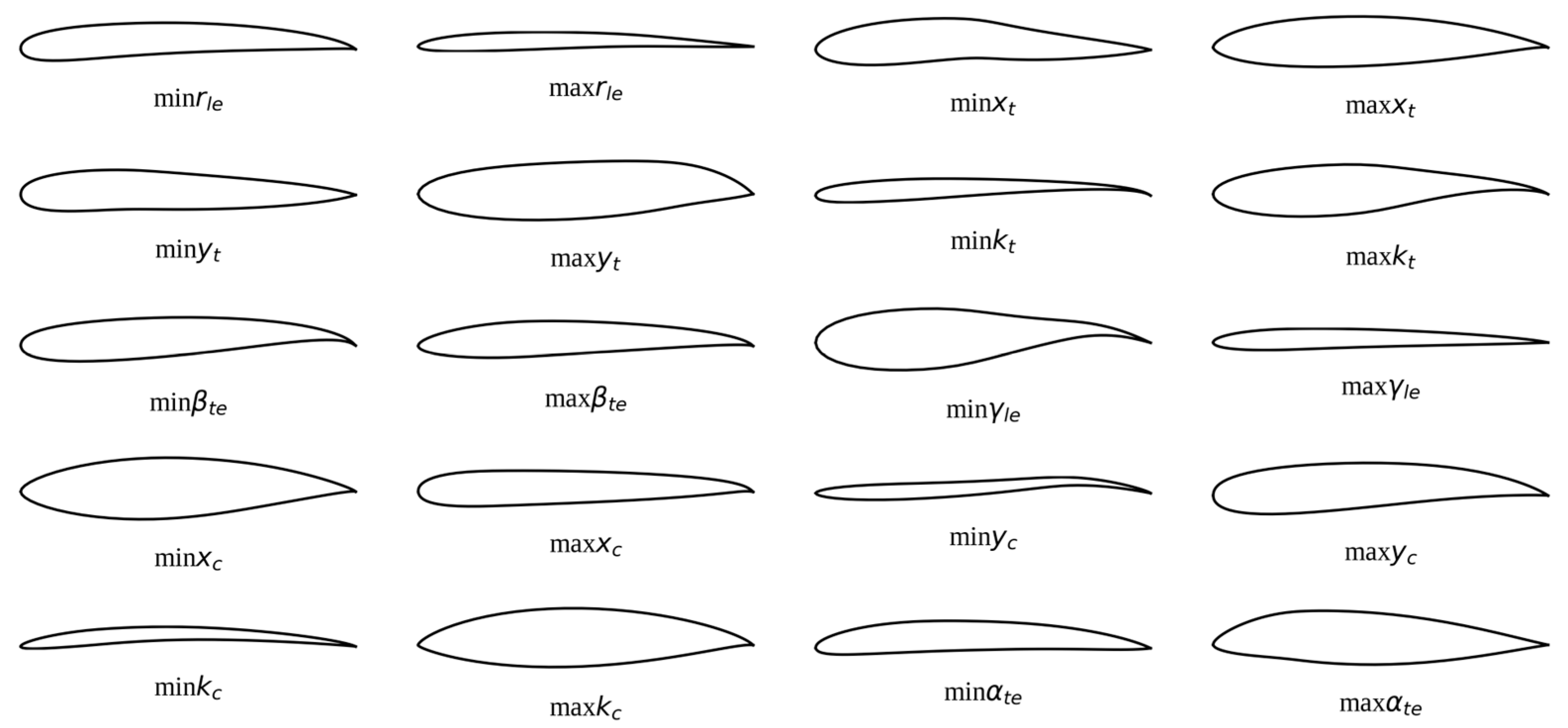
The use of MLP models requires a large amount of high-quality data to adjust and optimize the weight values of the neurons during training. In this work, the input values and intervals of each parameter were chosen to cover as much of the design space as possible. The intervals for the BP3333 parameters, which determine the profile geometry, were derived from the study conducted in the work [27]. Table 3 shows the ranges of each BP3333 parameter, which can model almost any asymmetric general aviation airfoil, such those belonging to different families or series, such as Eppler, NACA, Gottingen, TsAGI, etc. [16,22,27]. An evolutionary optimization algorithm was used to obtain the intervals of each BP3333 parameter. The goal of the optimization was to model 800 asymmetric airfoils from the University of Illinois at Urbana-Champaign (UIUC) airfoil database [28].
The dzte and zte ranges are not indicated in Table 3 because they maintain a constant value of 0.001 and 0.0, respectively, which allowed us to reduce the number of parameters needed to define the profile geometry to 10. In addition to the 800 airfoils in the UIUC database, Figure 3 shows other examples of airfoils that can be created from the intervals indicated in Table 3. These airfoils were randomly generated for the database, and the intention of presenting them in Figure 3 is to demonstrate the limits of the range of each BP3333 parameter.
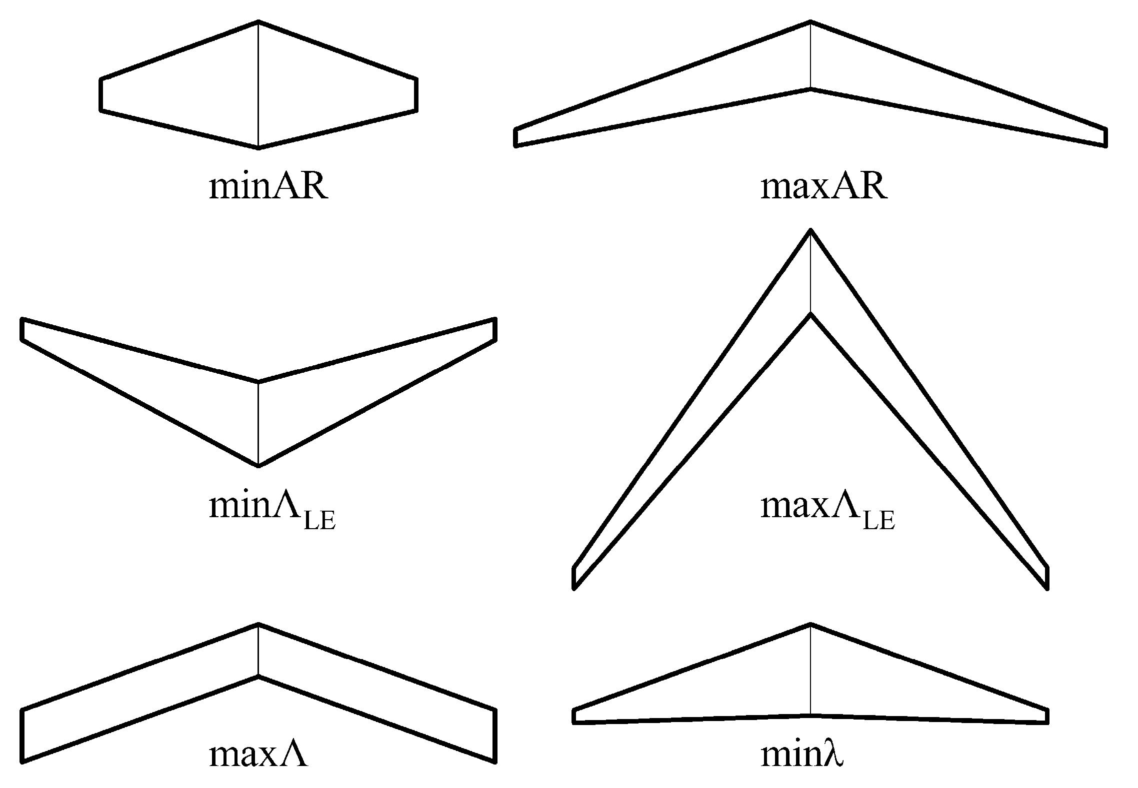
The intervals that determine the wing configuration are shown in Table 4. Figure 4 shows some examples of top-view wing geometries that can be created from the intervals indicated in Table 4. The minimal value of the aspect ratio is 4, since the VLM returns feasible results above this value [25]. In the case of the flight velocity, the maximum velocity corresponds to a Mach number of 0.6 at sea level. The angle of attack was restricted to the lineal part of the lift curve.
To ensure the performance of the MLP model, it is important to normalize the intervals of all parameters between 0 and 1 before training. To obtain a representative sample of the design space, a commonly used method is Latin hypercube sampling (LHS) [17,29]. However, due to limitations in the parameterization method used for generating profile geometries, the LHS method cannot be applied to the entire design space of 18 proposed variables. Instead, a combination of conventional uniform random sampling and LHS was used to create the databases. The samples from the subspaces formed by the BP3333 parameters were selected using conventional random sampling and were restricted by the design restrictions imposed by the mathematical model. Meanwhile, samples from the subspaces defined by the wing configuration and flight characteristics were selected using LHS.
The quality of the output data depends on the performance of the mathematical model used to calculate them. In this work, the quality of the output parameters is a function of the performance of the discrete vortex method implemented in AVL, along with empirical equations, particularly the analysis of inviscid compressible steady flow acting on the wing surface.
One of the crucial factors in creating a database for training a deep learning model is determining the amount of data required for optimal performance. To evaluate this, learning curves, also known as training curves, can be used. These plots show the relationship between the optimal value of the loss function for a given training set and the loss function evaluated on a validation dataset using the same parameters. By analyzing these curves, it is possible to determine how much a model benefits from additional training data, as well as if the model is suffering from high variance or high bias. If both the validation score and the training score converge to a low value as the training set size increases, it is unlikely that adding more data will improve performance.
After determining the optimal architecture and validating the performance of the network based on the number of data, learning curves were implemented. To perform optimization processes for two of the MLP hyperparameters, a database size of 1000 was defined as the minimum sample. To realize the learning curve, the size of the database was doubled (1000, 2000, 4000, etc.) until convergence was found.

2.2.2. MLP Hyperparameters Determination

An MLP is type of feedforward neural network in which the output of one layer is connected to all the neurons of the next layer. The output of layer L, denoted as aL, is a nonlinear transformation of the weighted sum of outputs aL−1 of the (L−1)th layer, including a bias term bL−1. The mathematical expression of a single neuron of the MLP is the following:
zL = ΘL aL−1 + bL−1,
aL = g(zL),
where L ∈ [1, N]. If the network has sL−1 neurons in layer L−1, and sL neurons in layer L, ΘL−1 is defined as the weight matrix having sL∙(sL−1 + 1) dimensions. This weight matrix can be intuitively thought of as structure that maps the output values of layer L−1 to layer L, where g(zL) is defined as a vector of outputs of individual neurons based on a nonlinear activation function. The final output of nested functions that make up an NL-layered MLP is aNL, where a0 is the input vector. The training of MLPs is typically conducted using the backpropagation algorithm. The backpropagation algorithm minimizes a loss function using common optimization algorithms [9,17].
The hyperparameters that define an MLP are the number of layers, number of neurons, activation function, loss function, optimizer, learning rate, number of epochs, and batch size. In this work, only two optimization processes are proposed: to obtain the best values for the number of hidden layers and the number of neurons per layer. The characteristics and values of the hyperparameters are held constant throughout all the analyses. The characteristics are the following:
  • The activation function for all hidden layers was the rectified linear unit (RELU) function due to its computational simplicity and effectiveness in handling of vanishing gradients [9].
  • The output layer was composed of two concatenated layers with different activation functions: the first sublayer was composed of a neuron (CD) with the exponential linear unit (ELU) function [30], which prevents predictions from being less than zero; this is of extreme importance, since physically, the CD value is never less than zero. The second sublayer is composed of two neurons (CL and CM) with the linear function.
  • The mean square error (MSE) was chosen as the loss function, which is commonly used for regression analysis. Since the MSE often refers to the mean squared prediction error or out of the sample mean squared error, it can refer to the mean of the squared deviations of the predictions of the true values, over a space outside the test sample, generated by an estimated model during a particular sample space [9,18,31].
  • The optimizer chosen was adaptive moment estimation (Adam), which is an algorithm for first-order gradient-based optimization of stochastic objective functions, based on adaptive estimates of lower-order moments. The method is straightforward to implement, is computationally efficient, has few memory requirements, is invariant to diagonal rescaling of the gradients, and is well suited for problems that are large in terms of data and/or parameters. The method is also appropriate for nonstationary objectives and problems with very noisy and/or sparse gradients [32].
  • The learning rate was fixed at 0.001, predetermined by the Adam optimizer function in Keras [33].
  • A total of 100 epochs were used for evaluation of the MLP, which has been sufficient in similar works [9,18].
  • A batch size of 20 was chosen for all evaluations, as is not expected to use very large database sizes (above the order of 104).
The performance of each network is evaluated using two metrics: root mean square error (RMSE) and the coefficient of determination (R2). RMSE measures the standard deviation of the residuals or prediction errors, while R2 is a statistical measure of how well the regression predictions approximate the real data points. To determine the optimal values of the hyperparameters, the performance of the architectures is compared using the average of these metrics obtained by cross-validation method. The chosen variant of cross-validation is K-fold cross-validation, which improves the holdout method by ensuring that the model score does not depend on how the training and test sets were chosen. The sample data are divided into K subsets, with one subset used as test data and the rest (K−1) as training data. The cross-validation process is repeated for K iterations, using each of the possible subsets of test data, as shown in Figure 5. The final result is obtained by taking the arithmetic mean and standard deviation of the results from each iteration. The number of iterations used in practice depends on the size of the data set, with 10 iterations being common and a minimum of 5 iterations used [20,34]. In this case, only 5 subsets were used. Therefore, the averaged metrics, particularly RMSE, provided by the K-fold cross-validation method will be used to define the final architecture.
The process to define the two remaining hyperparameters was as follows:
  • The number of hidden layers was determined by evaluating five architectures, ranging from one to five hidden layers. Each architecture was assigned 64 neurons per layer.
  • To define the number of neurons per layer, the integer encoding differential evolution (IEDE) algorithm was used. This algorithm was used because it uses integer variables. The number of variables corresponds to the number of hidden layers obtained in the previous process. The IEDE algorithm, like the DE algorithm, consists of three evolutionary operators: mutation, crossover, and selection. These operators can be observed in more detail in Algorithm A1 [20], which is provided in Appendix A. The mutation operator operates with a scale factor (F) of 0.85, while the crossover operator requires a crossover constant (CR) of 0.85. Other initial parameters of the algorithm include: number of variables (D), which is based on the number of hidden layers determined in the previous process; the design interval of each variable ([Dmin, Dmax]) [9,16]; the population size of each generation (N), which was set to 10 times the number of variables; the cost function to be minimized (f), defined by the average RSME value provided by the k-fold cross-validation method; and the stopping condition, which was set as a limit of 20 generations (G = 20).
Finally, the MLP with the selected optimal architecture was trained using four different database sizes. These MLPs were assessed by performing a “database-size independency” test, which involves choosing the smallest database that is capable of providing the best possible performance.
All the evaluated neural networks were programmed in Python3 using the Numpy, Scikit-Learn and Tensor Flow-Keras libraries. The specifications of the computer used for the training are provided in Table 5.

3. Results and Discussion

3.1. Databases

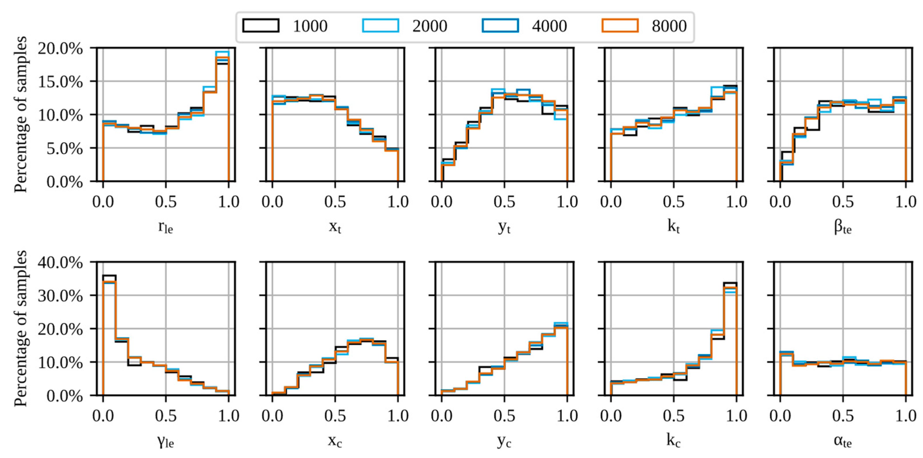
The distribution of each BP3333 parameter used in this work is shown in Figure 6. It can be observed that only one of the BP3333 parameters (αte) had a uniform distribution. Some other parameters, such as kc and γle, displayed a trend towards one of the extreme values of their respective ranges. However, it is important to note that each of the parameters displayed a consistent distribution based on the number of samples, which suggest that this trend may be maintained with larger amounts of sampling.
The LHS method was employed to create the vectors, with the remaining eight parameters describing the wing geometry and flight characteristics. However, some wing configurations presented complications when calculating their aerodynamic coefficients using the AMM, and had to be omitted and replaced with vectors selected through a conventional random sampling method.
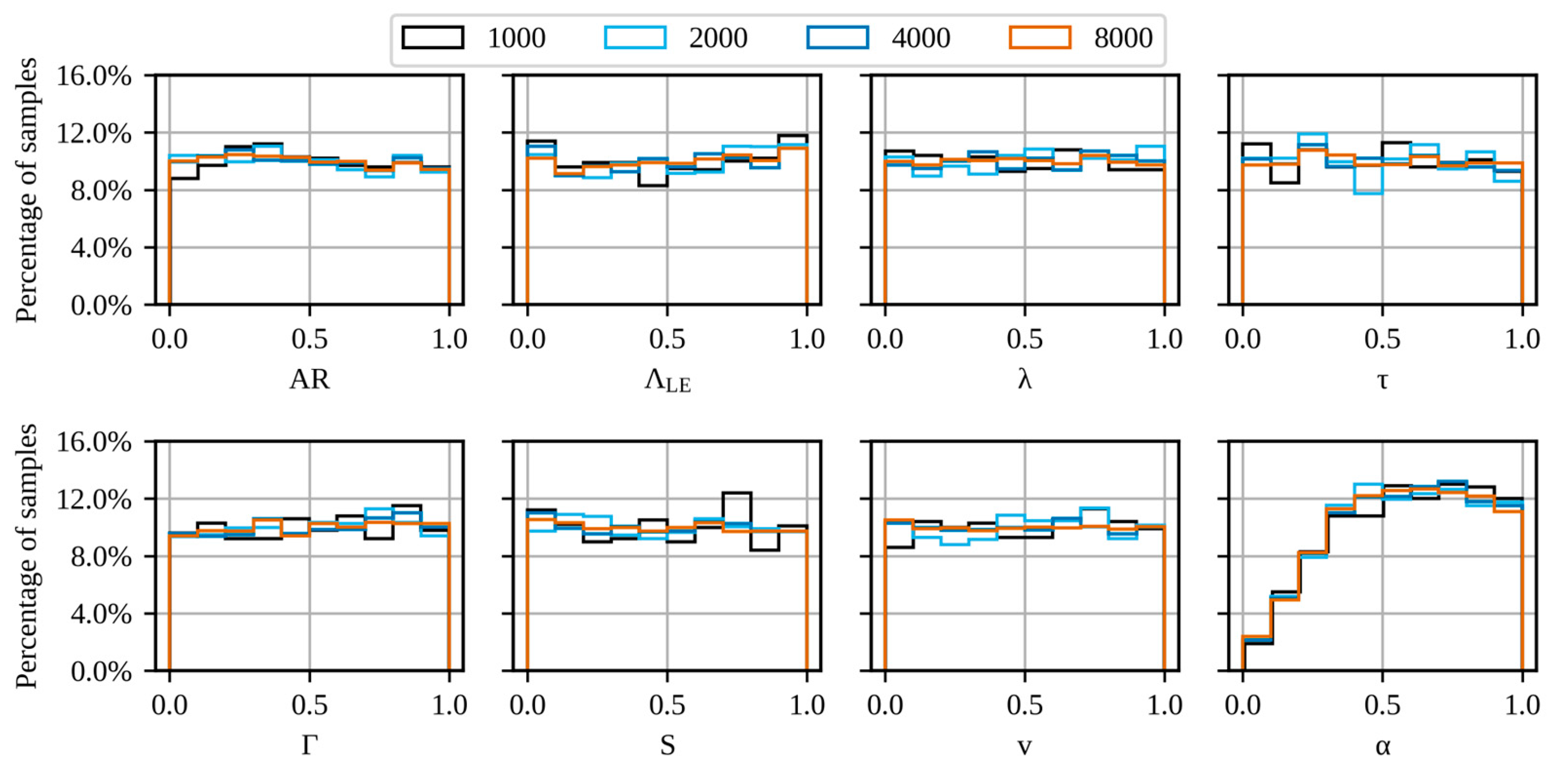
As seen in Figure 7, the parameters tend to have a uniform distribution across the different databases used, with the exception of the angle of attack. The low percentage of samples with minimum angles of attack is a result of filtering the CD values lower than 0.01, as it was initially believed that these values did not correspond to real-world values. Since low CD values are typically obtained at low angles of attack, filtering these vectors resulted in the elimination of the angles of attack corresponding to low CD values.

3.2. Hidden Layers Determination

Table 6 shows the averaged values of the loss function, and the average values and standard deviation of the metrics obtained from the k-fold cross-validation for each of the five evaluated architectures.
The configuration of four hidden layers shows a better performance in the RMSE metric. Although the five-layer hidden configuration shows slight improvements in the R2 metrics for the drag and momentum coefficients, it was decided to opt for the four-layer configuration as it is a less complex configuration. This configuration was highlighted in green in Table 6.

3.3. Neurons Number Determination

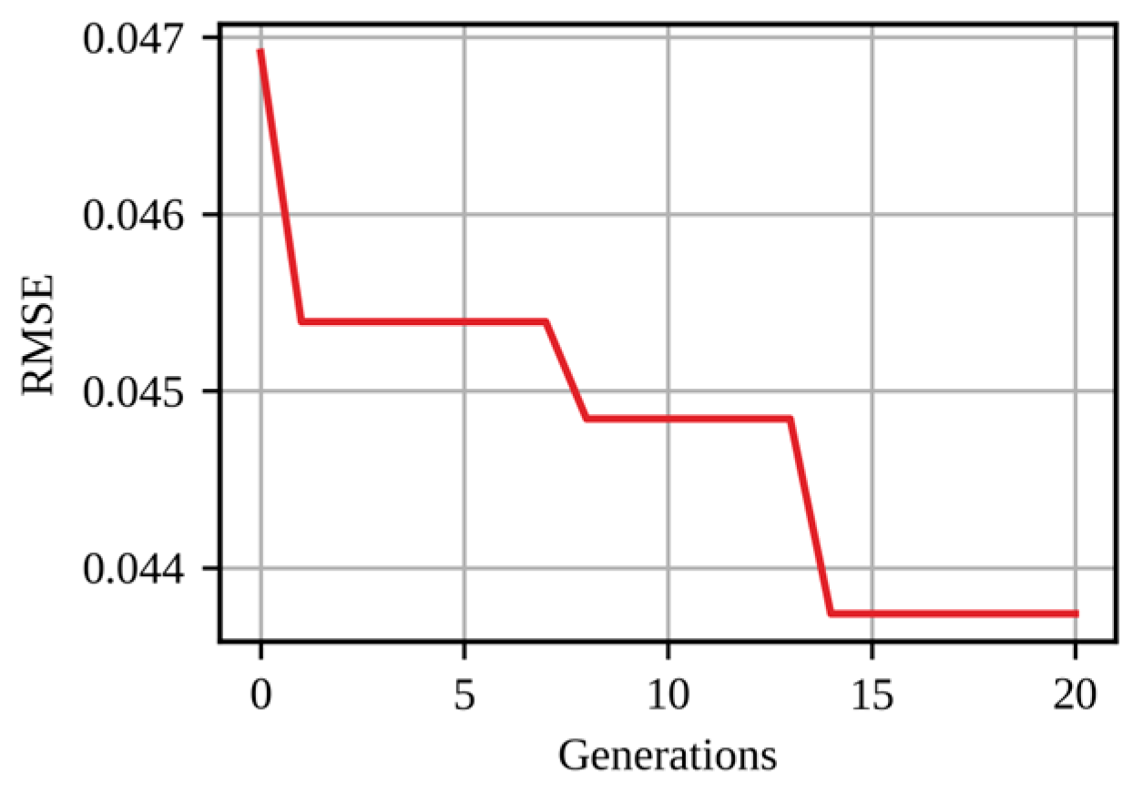
Once the number of hidden layers (four layers) had been selected, the parameters of the evolutionary algorithm, such as the number of variables (four variables) and the population size (forty individuals), could be defined. In Figure 8, it can be seen how the cost function was minimized using Algorithm A1.
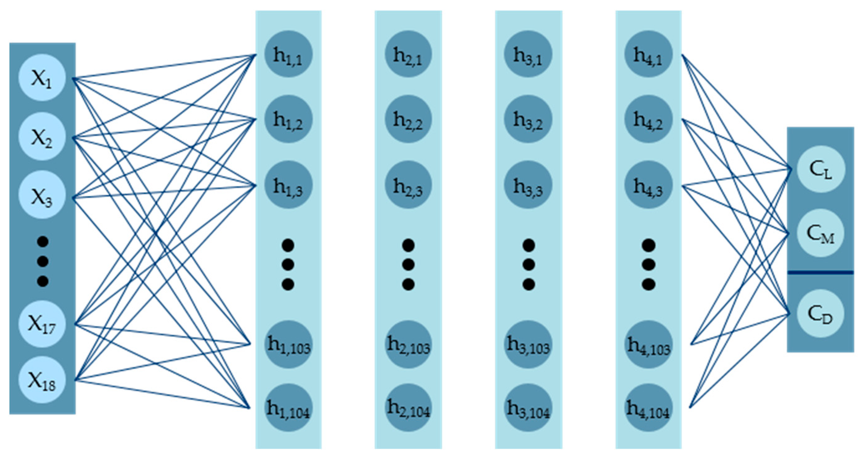
After 20 generations, the IEDE algorithm managed to minimize the RMSE to a value of 0.0438. This value was achieved with an architecture of four hidden layers: the first layer with 104 neurons, the second with 123 neurons, the third with 100 neurons, and the fourth with 109 neurons. Figure 9 shows graphically the optimized MLP architecture [33].

3.4. MLP Performance with Different Database Sizes

Having already defined the architecture of the MLP, we proceeded to analyze its performance based on the number of data used. Figure 10 shows the learning curve as a function of the RMSE and Table 7 shows the mean and standard deviation values of the cost function and the metrics.
As can be seen from Table 7, between 4000 and 8000 data used, there is no significant difference in the value of MSE. There are slight advantages of using 8000 data, especially for R2 for the drag coefficient. However, as can be seen in the learning curves (see Figure 10), the increase in the RMSE with 8000 data in the training and testing curves indicates an indication of overfitting. Therefore, it is considered that 4000 data are enough to have a good performance of the MLP for aerodynamic coefficient prediction (3200 data for training and 800 for testing). We have highlighted the selected architecture with green color for its ease of identification.
Using the best values of weights obtained during the cross-validation process and a database with 4000 data, a more detailed analysis of the prediction of the aerodynamic coefficients in the testing stage through regression analysis is shown in Figure 11. In a regression analysis, the coefficients predicted by the MLP are compared with the coefficients obtained by AMM. For an ideal MLP, the predicted coefficients (P) coincide exactly with the calculated coefficients (T). This is represented graphically by the dotted line T=P. The scatters closer to T=P represent a better prediction [16].
The regression analysis and the absolute error of the testing data are presented in Figure 11 and Figure 12, respectively. As a result, we obtained a good R2 (>0.9 [16]) in the order of 0.9877 for CD, 0.9966 for CL, and 0.9988 for CM (see Figure 11). It is noticeable that the prediction accuracy of the CD is worse than the CL and CM; this can be explained as the result of using empirical formulas for computing parasitic drag. As the total drag is calculated as the sum of the induced and parasitic drag, then the latter disturbs the value of the total drag.

3.5. Computing Performance

The computing performance of the MLP was compared against the substituted AMM in groups of 10, 100, and 1000. In Table 8 the geometric characteristics and flight conditions are presented, and in Table 9, of the group of 10 wings is presented for a clear presentation of results.
The specification of the computer used for the comparison are shown in Table 2. The MLP and AMM execution time is presented in Table 10.
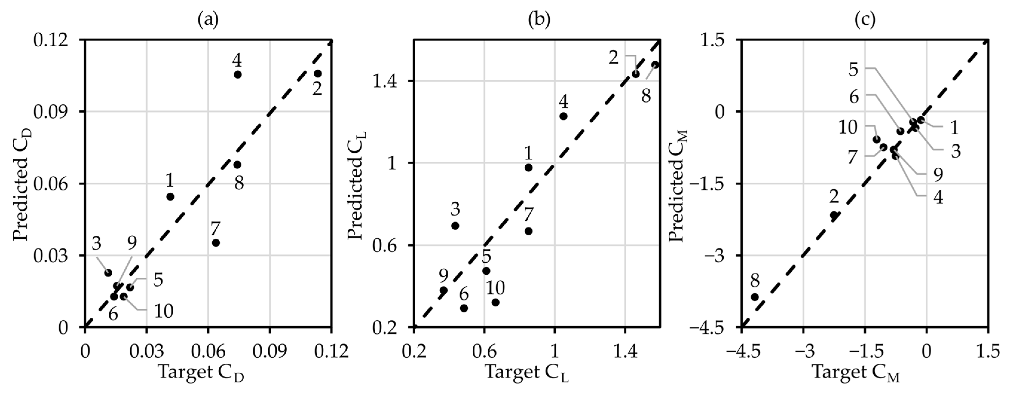
The increment of the computing time for the AMM is linear due to its sequential execution, while the computing time of the MLP is almost linear. Since the MLP executes predictions in parallel computation, the execution time improves if a large array of data is to be evaluated in comparison to the AMM. In Figure 13, the aerodynamic coefficients predicted and target value, as well as the MLP best line fit, are shown.

4. Conclusions

The method proposed in this article proved to be efficient for the design and training of an MLP for steady nonlinear aerodynamic response predictions. The developed MLP for the construction of a surrogate aerodynamics model allowed for the calculation of the integral aerodynamic characteristics of wings of different geometry under different flight conditions allowed with sufficiently high accuracy (R2 up to 0.9877, 0.9966, and 0.9988 for CD, CL, and CM respectively), as well as significantly reducing the required time and computing costs (by 1 and 2 orders of magnitude for arrays of 10 and 100 variants) in comparison with numerical mathematical models based on the vortex lattice method and empirical equations. It could be observed that the methodology implemented to define the MLP architecture was adequate; the implementation of cross validation processes, learning curves and evolutionary algorithms were substantial to determine some of the MLP hyperparameters. Much greater gains in computational and time costs can be obtained in comparison with the use of numerical modeling methods of aerodynamics based on the solution of Navier–Stokes equations. The significant acceleration of the aerodynamic characteristics calculation will allow one to use the proposed approach to perform optimization calculations at the initial stages of design, when there is a need to consider a large number of combinations of design variables in a wide range of values due to insufficient information and a large degree of uncertainty. We have some recommendations for improving the quality of the AMM used for generating the database, as well as the development of the MLP architecture. It would be possible to extend the upper limit of the angle of attack and hence accounting for stalling of the wing by incorporating a correction factor based on the Kirchhoff flow model, and to improve the CD calculation by adding additional terms for accounting other types of drag. Regarding the MLP, it could be further improved by using a learning rate scheduler and performing analysis of the number of epochs and batches, as well as a normalization of all input and output data between 0 and 1.
Future works will be focused on extending the capabilities of this surrogate model, building MDO algorithms for the initial stages of aircraft design, and employing this surrogate model for MDO and robust optimization.

Author Contributions

Conceptualization, O.U.E.B., J.G.Q.P. and O.L.; methodology, J.G.Q.P.; software, O.U.E.B. and J.G.Q.P.; validation, O.U.E.B. and J.G.Q.P.; formal analysis, J.G.Q.P.; investigation, O.U.E.B., J.G.Q.P. and O.L.; resources, E.K.; data curation, O.U.E.B. and J.G.Q.P.; writing—original draft preparation, O.U.E.B. and J.G.Q.P.; writing—review and editing, E.K. and O.L.; visualization, O.U.E.B. and J.G.Q.P.; supervision, O.L.; project administration, E.K. and O.L.; funding acquisition, E.K. All authors have read and agreed to the published version of the manuscript.

Funding

The study was financially supported by the Russian Science Foundation, project No. 22-79-10309.

Data Availability Statement

The data that support the findings of this study are available from the corresponding author, O.U.E.B., upon reasonable request.

Conflicts of Interest

The authors declare no conflict of interest. The funders had no role in the design of the study; in the collection, analyses, or interpretation of data; in the writing of the manuscript; or in the decision to publish the results.

Appendix A

The integer encoded differential evolution algorithm (IEDE) is an adaptation of the differential evolution (DE) algorithm for use in integer optimization problems. Algorithm A1 presents IEDE with its respective evolutionary operators (mutation, crossover, and selection) adapted to the encoding of integer variables.
Algorithm A1. IEDE algorithm.
Input: N, d, [Dmin, Dmax], F, CR, G
Output: xopt, fopt
Initialize the population randomly Pg = P(randint(x1,g,…,xN,g));
Calculate f(x1,g,…,xN,g) with k-fold cross-validation method
for g = 1 to G do
    for i = 1 to N do //Mutation
       Choosing xr1, xr2 and xr3 vectors randomly from Pg without replacement;
       δ = F (xr2 – xr3);
       for j = 1 to D do
          if rand() < δj – int ↑ (δj) then
             vj,i,g = xj,r1 + int ↑ (δj);
          else
             vj,i,g = xj,r1 + int ↓ (δj);
          end if
       end for
    end for
    for i = 1 to N do //Crossover
       for j = 1 to d do
          if rand() < CR or j == randint([0, d]) then
             uj,i,g = vj,i,g;
          else
             uj,i,g = xj,i,g;
          end if
       end for
    end for
    Calculate f(u1,g,…,uN,g) with k-fold cross-validation method;
    for i = 1 to N do //Selection
       if f(ui,g) ≤ f(xi,g) then
          xi,g+1 = ui,g;
       else
          xi,g + 1 = xi,g;
       end if
    end for
end for

References

  1. Poghosyan, M.; Liseytsev, N.; Strelets, D.; Kiselev, V.; Tarasov, A.; Dolgov, O.; Dudar, E.; Timoshenko, V.; Eremin, N.; Penkov, E.; et al. Aircraft Design, 5th ed.; Pogosyan, M., Liseytsev, N., Strelets, D., Eds.; Innovatsionnoye Mashinostroyeniye: Moscow, Russia, 2018; ISBN 978-5-6040281-5-5. [Google Scholar]
  2. Roskam, J. Airplane Design. Part V: Component Weight Estimation; DARcorporation: Lawrence, KS, USA, 2018; ISBN 9781884885693. [Google Scholar]
  3. Torenbeek, E. Advanced Aircraft Design: Conceptual Design, Technology and Optimization of Subsonic Civil Airplanes; Wiley: Hoboken, NJ, USA, 2013; ISBN 978-1-118-56811-8. [Google Scholar]
  4. Keane, A.J.; Nair, P.B. Computational Approaches for Aerospace Design: The Pursuit of Excellence; Wiley: Hoboken, NJ, USA, 2005; ISBN 0470855401. [Google Scholar]
  5. Martins, J.R.R.A. Aerodynamic Design Optimization: Challenges and Perspectives. Comput. Fluids 2022, 239, 105391. [Google Scholar] [CrossRef]
  6. Schulz, V.; Schillings, C. Optimal Aerodynamic Design under Uncertainty. In Management and Minimisation of Uncertainties and Errors in Numerical Aerodynamics: Results of the German Collaborative Project MUNA; Eisfeld, B., Barnewitz, H., Fritz, W., Thiele, F., Eds.; Springer Berlin: Berlin, Germany, 2013; pp. 297–338. ISBN 978-3-642-36185-2. [Google Scholar]
  7. Peng, X.; Zhu, H.; Xu, D.; Xiao, M.; Wang, W.; Cai, G. Aerodynamic Performance Uncertainty Analysis and Optimization of a Conventional Axisymmetric Vehicle Based on Parallel Polynomial Chaos Expansions. Aerospace 2022, 9, 396. [Google Scholar] [CrossRef]
  8. Mavris, D.N.; Pinon, O.J. An Overview of Design Challenges and Methods in Aerospace Engineering. In Complex Systems Design & Management; Springer Berlin: Berlin, Germany, 2012; pp. 1–25. [Google Scholar]
  9. Moin, H.; Khan, H.Z.I.; Mobeen, S.; Riaz, J. Airfoil’s Aerodynamic Coefficients Prediction Using Artificial Neural Network. arXiv 2021, arXiv:2109.12149v1. [Google Scholar]
  10. Balla, K.; Sevilla, R.; Hassan, O.; Morgan, K. An Application of Neural Networks to the Prediction of Aerodynamic Coefficients of Aerofoils and Wings. Appl. Math. Model 2021, 96, 456–479. [Google Scholar] [CrossRef]
  11. Huang, S.; Miller, L.; Steck, J. An Exploratory Application of Neural Networks to Airfoil Design; American Institute of Aeronautics and Astronautics (AIAA): Reston, VA, USA, 1994. [Google Scholar]
  12. Sun, G.; Sun, Y.; Wang, S. Artificial Neural Network Based Inverse Design: Airfoils and Wings. Aerosp. Sci. Technol. 2015, 42, 415–428. [Google Scholar] [CrossRef]
  13. Yang, S.; Lee, S.; Yee, K. Inverse Design Optimization Framework via a Two-Step Deep Learning Approach: Application to a Wind Turbine Airfoil. Eng. Comput. 2022. [Google Scholar] [CrossRef]
  14. Khurana, M.S.; Winarto, H.; Sinha, A.K. Application of Swarm Approach and Artificial Neural Networks for Airfoil Shape Optimization the Direct Numerical Optimization (DNO) Approach for Airfoil Shape Design Requires the Integration of Modules: A) A Geometrical Shape Function; b). In Proceedings of the 12th AIAA/ISSMO Multidisciplinary Analysis and Optimization Conference, Victoria, BC, Canada, 10–12 September 2008. [Google Scholar]
  15. Bouhlel, M.A.; He, S.; Martins, J.R.R.A. Scalable Gradient–Enhanced Artificial Neural Networks for Airfoil Shape Design in the Subsonic and Transonic Regimes. Struct. Multidiscip. Optim. 2020, 61, 1363–1376. [Google Scholar] [CrossRef]
  16. Kharal, A.; Saleem, A. Neural Networks Based Airfoil Generation for a given Cp Using Bezier-PARSEC Parameterization. Aerosp. Sci. Technol. 2012, 23, 330–344. [Google Scholar] [CrossRef]
  17. Secco, N.R.; de Mattos, B.S. Artificial Neural Networks to Predict Aerodynamic Coefficients of Transport Airplanes. Aircr. Eng. Aerosp. Technol. 2017, 89, 211–230. [Google Scholar] [CrossRef]
  18. Elgeldawi, E.; Sayed, A.; Galal, A.R.; Zaki, A.M. Hyperparameter Tuning for Machine Learning Algorithms Used for Arabic Sentiment Analysis. Informatics 2021, 8, 79. [Google Scholar] [CrossRef]
  19. Hu, L.; Zhang, J.; Xiang, Y.; Wang, W. Neural Networks-Based Aerodynamic Data Modeling: A Comprehensive Review. IEEE Access 2020, 8, 90805–90823. [Google Scholar] [CrossRef]
  20. Deng, C.; Zhao, B.; Yang, Y.; Deng, A. Integer Encoding Differential Evolution Algorithm for Integer Programming. In Proceedings of the 2010 2nd International Conference on Information Engineering and Computer Science, Wuhan, China, 25–26 December 2010; pp. 1–4. [Google Scholar]
  21. Pedregosa, F.; Varoquaux, G.; Gramfort, A.; Michel, V.; Thirion, B.; Grisel, O.; Blondel, M.; Müller, A.; Nothman, J.; Louppe, G.; et al. Scikit-Learn: Machine Learning in Python. arXiv 2012. [Google Scholar] [CrossRef]
  22. Derksen, R.W.; Rogalsky, T. Bezier-PARSEC: An Optimized Aerofoil Parameterization for Design. Adv. Eng. Softw. 2010, 41, 923–930. [Google Scholar] [CrossRef]
  23. Drela, M.; Youngren, H. MIT AVL User Primer—AVL 3.36 1–43. Available online: https://web.mit.edu/drela/Public/web/avl/ (accessed on 5 February 2023).
  24. Kholyavko, V. Calculation of the Aerodynamic Characteristics of the Aircraft. Part 1; Kharkiv Aviation Institute: Kharkiv, Ukraine, 1991. [Google Scholar]
  25. Espinosa Barcenas, O.U.; Quijada Pioquinto, J.G.; Kurkina, E.; Lukyanov, O. Multidisciplinary Analysis and Optimization Method for Conceptually Designing of Electric Flying-Wing Unmanned Aerial Vehicles. Drones 2022, 6, 307. [Google Scholar] [CrossRef]
  26. Anderson, R.F. Determination of the Characteristics of Tapered Wings; National Advisory Committee for Aeronautics: Boston, MA, USA, 1937.
  27. Quijada Pioquinto, J.G.; Shakhov, V. Acceleration of Evolutionary Optimization for Airfoils Design with Population Size Reduction Methods. In Proceedings of the 20th International Conference “Aviation and Cosmonautics”, Samara, Russia, 22–26 November 2021. [Google Scholar]
  28. Selig, M. UIUC Airfoil Data Site. Available online: https://m-selig.ae.illinois.edu/ads/coord_database.html (accessed on 5 May 2022).
  29. McKay, M.D.; Beckman, R.J.; Conover, W.J. A Comparison of Three Methods for Selecting Values of Input Variables in the Analysis of Output from a Computer Code. Technometrics 1979, 21, 239. [Google Scholar] [CrossRef]
  30. Clevert, D.-A.; Unterthiner, T.; Hochreiter, S. Fast and Accurate Deep Network Learning by Exponential Linear Units (ELUs). arXiv 2015, arXiv:1511.07289v5. [Google Scholar]
  31. Quadros, J.D.; Khan, S.A.; Aabid, A.; Alam, M.S.; Baig, M. Machine Learning Applications in Modelling and Analysis of Base Pressure in Suddenly Expanded Flows. Aerospace 2021, 8, 318. [Google Scholar] [CrossRef]
  32. Kingma, D.P.; Ba, J. Adam: A Method for Stochastic Optimization. arXiv 2014, arXiv:1412.6980v9. [Google Scholar]
  33. Chollet, F. Others Keras. 2015. Available online: https://github.com/fchollet/keras (accessed on 5 February 2023).
  34. Berrar, D. Cross-Validation. In Encyclopedia of Bioinformatics and Computational Biology; Elsevier: Amsterdam, The Netherlands, 2019; pp. 542–545. [Google Scholar]
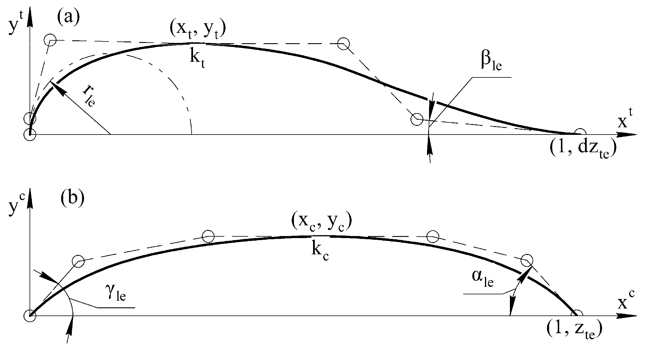
Figure 1. Parameters BP3333 and Bezier control points: (a) thickness curve; (b) camber curve.
Aerospace 10 00149 g001
Figure 2. Comparison between AMM and experimental obtained lift and drag coefficients and lift-to-drag ratio.
Aerospace 10 00149 g002
Figure 3. Examples of airfoils that could be generated with BP3333 parameters within the given interval.
Aerospace 10 00149 g003
Figure 4. Examples of wings that could be generated with the AR, ΛLE, and λ within the given interval.
Aerospace 10 00149 g004
Figure 5. Form of selection of the database for testing with the k-fold cross-validation process [20,34].
Aerospace 10 00149 g005
Figure 6. Distribution of each of the BP3333 parameters for different database sizes.
Aerospace 10 00149 g006
Figure 7. Distribution of each of the wing parameters and flight conditions for different database sizes.
Aerospace 10 00149 g007
Figure 8. Cost function convergence for the optimization of the number of neurons per layer.
Aerospace 10 00149 g008
Figure 9. Model of the optimized MLP architecture.
Aerospace 10 00149 g009
Figure 10. MLP learning curve.
Aerospace 10 00149 g010
Figure 11. Regression analysis of the final MLP architecture at the testing stage: (a) drag coefficient; (b) lift coefficient; (c) pitch moment coefficient.
Aerospace 10 00149 g011
Figure 12. Absolute error of the testing data; (a) drag coefficient; (b) lift coefficient; (c) pitch moment coefficient.
Aerospace 10 00149 g012
Figure 13. Comparison between the calculated and predicted aerodynamic coefficients of the group of 10 wings: (a) drag coefficient; (b) lift coefficient; (c) pitch moment coefficient.
Aerospace 10 00149 g013
Table 1. MAE for lift coefficient, drag coefficient, and lift-to-drag-ratio of the AMM and k-Ω SST.
Aerodynamic CharacteristicMAE
AMMk-Ω SST
CL0.0290.008
CD0.0031390.006074
L/D3.294.73
Table 2. Specifications of the computer used for computing performance test.
Specifications
ProcessorIntel® CoreTM i7-6700 CPU @ 3.40 GHz x 8
Memory62 GB RAM
Hard disk500 GB
Operating systemGNU/Linux Ubuntu 20.04.4 LTS
Table 3. BP3333 parameter interval for representing general aviation airfoils.
BP3333 ParameterInterval
rle[−0.05, −0.001]
xt[0.2, 0.45]
yt[0.02, 0.12]
kt[−0.9, −0.2]
βte[0.01, 0.4]
γle[0.002, 0.04]
xc[0.2, 0.85]
yc[0.005, 0.07]
kc[−1.75, −0.025]
αte[0.002, 0.7]
Table 4. Wing geometric characteristics and flight condition interval.
Wing Geometric Characteristics and Flight ConditionsInterval
AR[4, 14]
ΛLE, °[−15, 55]
λ[0.143, 1]
τ, °[−5, 2]
Γ, °[−3, 9]
S, m2[10, 100]
v, m/s[10, 204]
α, °[−5, 15]
Table 5. Specifications of the computer used for the MLP training.
Specifications
ProcessorIntel® CoreTM i9−9940 CPU @ 3.30 GHz x 14
Memory125 GB RAM
Hard disk2 TB
Operating systemGNU/Linux Ubuntu 18.04.5 LTS
Table 6. Hidden layers number analysis.
ArchitectureMSERMSE R2
CDCLCM
18-64-30.00560.0750
±0.0279
0.8621
±0.0944
0.9503
±0.0355
0.9760
±0.0106
18-64-64-30.00280.0525
±0.0291
0.9287
±0.0389
0.9776
±0.0119
0.9877
±0.0081
18-64-64-64-30.00230.0483
±0.0272
0.8987
±0.0573
0.9777
±0.0136
0.9899
±0.0071
18-64-64-64-64-30.00220.0479
±0.0202
0.9192
±0.0348
0.9809
±0.0137
0.9899
±0.0097
18-64-64-64-64-64-30.00260.0514
±0.0207
0.9205
±0.0357
0.9720
±0.0178
0.9911
±0.0060
Table 7. Database size analysis.
Database SizeMSERMSER2
CDCLCM
10000.00190.0438
±0.0200
0.9527
±0.0193
0.9842
±0.0101
0.9911
±0.0080
20000.00150.0387
±0.0161
0.9609
±0.0167
0.9866
±0.0102
0.9919
±0.0081
40000.00090.0304
±0.0096
0.9772
±0.0097
0.9916
±0.0043
0.9961
±0.0026
80000.00100.0325
±0.0091
0.9733
±0.0105
0.9916
±0.0028
0.9960
±0.0022
Table 8. Geometric characteristics and flight conditions of the group of 10 wings.
Top ViewARLeading-Edge
Sweep Angle, °
Taper
Ratio
Dihedral
Angle, °
Twist
Angle, °
Wing
Area, m2
Velocity,
m/s
Angle of Attack, °
1 Aerospace 10 00149 i0017.25−13.30.198−1.5−4.121.250102.155.5
2 Aerospace 10 00149 i0026.7539.30.3775.10.834.75082.7513.5
3 Aerospace 10 00149 i00311.25−2.80.2413.9−4.512.25024.55−0.5
4 Aerospace 10 00149 i0045.2521.80.2251.5−0.393.250199.1510.5
5 Aerospace 10 00149 i0057.750.80.187−0.91.116.750150.651.5
6 Aerospace 10 00149 i0069.7518.30.3088.1−3.139.250131.25−1.5
7 Aerospace 10 00149 i0074.2542.80.4266.30.466.25034.259.5
8 Aerospace 10 00149 i00812.2546.30.168−2.1−1.043.750179.7511.5
9 Aerospace 10 00149 i0096.2553.30.2827.5−2.797.750121.552.5
10 Aerospace 10 00149 i01011.7532.30.1465.71.584.25092.450.5
Table 9. Airfoil BP3333 parameters of the group of 10 wings.
Airfoilrlextytktβteγlexcyckcαte
1 Aerospace 10 00149 i011−0.02150.36170.0881−0.73340.36850.02620.71310.0396−0.61380.4248
2 Aerospace 10 00149 i012−0.00240.35070.0718−0.76820.28990.02840.75910.0264−0.47280.4370
3 Aerospace 10 00149 i013−0.00800.41720.0575−0.37470.25160.15730.60860.0362−0.04040.5869
4 Aerospace 10 00149 i014−0.02580.35110.0876−0.41840.34820.01090.65350.0274−0.79950.4292
5 Aerospace 10 00149 i015−0.02880.22100.0529−0.62470.39990.02440.49860.0304−0.53580.2399
6 Aerospace 10 00149 i016−0.02880.34060.0898−0.87680.39730.01500.60090.0368−1.07490.1877
7 Aerospace 10 00149 i017−0.01630.25600.0613−0.65300.15330.05090.34750.0296−0.69150.0272
8 Aerospace 10 00149 i018−0.01730.27310.0583−0.75520.22240.05300.79710.0231−0.04220.6824
9 Aerospace 10 00149 i019−0.04320.30690.0824−0.29100.35480.04510.61340.0246−0.09500.2217
10 Aerospace 10 00149 i020−0.04020.27570.0721−0.31570.35540.08540.42470.0395−0.87550.0408
Table 10. Comparison of time requirement and speedup.
SpecificationsTime, s (Table 2 CPU)Speedup
AMM simulation for one case0.141-
Training: MLP with k-fold cross validation31.315-
Prediction: Batch size = 100.1359.47
Prediction: Batch size = 1000.14090.42
Prediction: Batch size = 10000.159797.42
Disclaimer/Publisher’s Note: The statements, opinions and data contained in all publications are solely those of the individual author(s) and contributor(s) and not of MDPI and/or the editor(s). MDPI and/or the editor(s) disclaim responsibility for any injury to people or property resulting from any ideas, methods, instructions or products referred to in the content.