The Low Fuel Consumption Keeping Method of Eccentricity under Integrated Keeping of Inclination-Longitude

Abstract

The influence of the natural perturbation force will cause the eccentricity of the GEO satellite to produce a periodic motion with a period of years, and then cause the east–west station of the GEO satellite to oscillate. From the perspective of the best fuel-saving or the failure of the thruster used for station keeping, some scholars have proposed a method of slightly deflecting the thrust used for north–south station keeping (NSSK) to the east or west to achieve the integrated keeping of inclination and longitude. The disadvantage of this strategy is that the eccentricity cannot be maintained, and even causes the continuous divergence of the eccentricity. Based on the above problems, this paper proposes a low fuel consumption keeping method for eccentricity under the integrated maintenance of inclination and longitude. Assuming that the satellite is only equipped with a south (north) direction thruster for station keeping, on the premise of not affecting the satellite’s Earth observation, the satellite’s forward flight and backward flight are switched every year at the spring equinox and autumn equinox, which can prevent the eccentricity divergence when performing mean longitude keeping. When the accuracy of the east–west station keeping is not pursued, this method can not only effectively save the fuel consumption of the station keeping, but also greatly reduce the number of eccentricity maintenance interventions and the interference to the whole satellite due to the eccentricity keeping, which has a certain engineering application value.

1. Introduction

Geosynchronous orbit (GEO) satellites [1,2] are high-orbit satellites located above the equator. They have the characteristics of wide ground coverage and fixed pointing to the ground, and are widely used in communication, navigation, and meteorological observation, as well as in other fields.

However, under the action of various natural perturbations, satellites in GEO will gradually drift away from their original orbits, which will not only reduce the work efficiency of satellites but may also cause satellites in GEO to collide. Therefore, orbital keeping of the GEO satellite is required on a regular basis to keep the GEO satellite near the designed orbital position. The station keeping (SK) of the GEO satellite is divided into north/south station keeping (NSSK) and east/west station keeping (EWSK). The NSSK is also called orbital inclination keeping, which is the out-of-plane control. The EWSK includes the mean longitude keeping and the eccentricity vector keeping. The change in the mean longitude will cause the change in the east–west center position of the GEO satellite. The change in the eccentricity will cause an oscillation in the east–west station of the GEO satellite [1,2].

Traditional GEO satellites use the method of chemical thrusters to realize the SK, and this control method is relatively mature. Zhang [3] used dual tangential thrust control to realize the EWSK and NWSK. It adopts the iterative shooting method to obtain the optimal orbital control interval that meets the requirements of positional accuracy. Simulation shows that this method can achieve a SK accuracy of 0.005°. Li [4,5] combined this with engineering practice and introduced several kinds of SK strategies for GEO satellites based on pulse thrust in detail, and analyzed the advantages, disadvantages, and uses of various SK strategies. Park [6], Li [7], Shi [8], etc. gave the co-location isolation strategy, the co-location strategy of multiple satellites, and the design method of the corresponding nominal orbit based on the eccentricity vector and orbital inclination vector. Shi [9] discussed the relationship between the orbital control period and the EWSK fuel consumption and gave an EWSK control strategy based on the pulse method. Li et al. [10,11,12] introduced the EWSK method based on a chemical thruster in detail, and successfully applied it on the Fengyun-2 satellite. No [13] designed the mean longitude keeping strategy based on dead zone control and the mean eccentricity keeping strategy based on the orbital eccentricity control by predicting the change in the mean eccentricity vector and realized the EWSK of the satellite. Yang [14] adopted the LQG (linear quadratic Gaussian) method to achieve an accuracy of the EWSK of 0.05° and an accuracy of the NWSK of 0.02°. Yang [15] drew on the idea of the “Deep Space One” intelligent autonomous control system structure and tried to design a GEO satellite SK strategy with strong autonomy. Vinod [16] designed an EWSK strategy based on perigee pointing to the Sun, which can effectively reduce the EWSK velocity increment. Chang [17] adopted the method of equally spaced pulses to divide the jet volume required for one EWSK into several smaller jets, which reduced the interference of a single jet on the satellite attitude and improved the control accuracy of the mean longitude. However, the control amount needs to be calculated and determined on the ground.

Considering the control accuracy and fuel consumption, some scholars have begun to study the use of micro-thrust for SK in recent years, and it has been applied to GEO satellites, such as Boeing 702 satellites [18,19]. Weiss et al. [20], Lin et al. [21], Caverly et al. [22], Weiss et al. [23], Walsh et al. [24], and others used the model prediction (MPC) method to realize the SK of the GEO satellites. This algorithm requires that the thrust of the electric thruster is required to be continuously adjustable, which requires too much computing power and is not friendly to spaceborne implementation. In addition, Frederik et al. [25], Gazzino et al. [26,27,28,29], Sukhanov et al. [30], Roth et al. [31], and others used various optimization algorithms to realize the SK of the GEO satellites.

In the literature [32,33], we have studied the method of the NSSK with high precision and low fuel consumption. In the process of the NSSK and the mean longitude keeping [32,33], in order to pursue the minimization of the fuel consumption, the integrated keeping of inclination–longitude is usually adopted. Compared with the separate control of NSSK and longitude keeping, the integrated keeping of inclination–longitude has the following characteristics:

(1)

It can save the fuel required for the mean longitude keeping;

(2)

The number of times of SK can be reduced;

(3)

The number of thrusters required is small, as only one thruster pointing in the north–south direction is required;

(4)

By maneuvering −5~5° in the yaw direction, the mean longitude can be kept.

However, the integrated control of inclination–longitude cannot achieve eccentricity keeping. By analyzing the movement of the eccentricity vector under the influence of natural perturbation, and according to the annual periodic motion law of the eccentricity vector [4,34], a control strategy for the eccentricity under the integrated keeping of inclination–longitude is proposed. The period for the satellite to switch the thrusters for the NSSK is one year, so that the natural drift period of the eccentricity in the uncontrolled state and the drift period of the longitude in the controlled state are both one year. The above two periodic terms are superimposed to form the “Equivalent Sun-pointing Eccentricity Vector”. By means of eccentricity adjustment, the eccentricity can be kept close to the “Equivalent Sun-pointing Eccentricity Vector”, thereby realizing the eccentricity vector keeping with low fuel consumption. The eccentricity keeping method proposed in this paper solves the problem of the eccentricity which cannot be kept under the control strategy of inclination–longitude integrated keeping. This method can not only save the velocity increment required for SK, but also reduces the number of SK times, simplifies the SK process, and reduces the influence of SK interference on the whole satellite, and can achieve high precision eccentricity keeping with only one thruster in the case of multiple thruster failure. Therefore, the eccentricity keeping method proposed in this paper has certain advantages in fuel consumption, reliability, and other aspects.

The structure of this paper is as follows. The calculation method of mean eccentricity and the periodic motion law of eccentricity under the action of perturbation are introduced in Section 1; the control method of eccentricity keeping is introduced in Section 2; the correctness of the method in this paper is verified by simulation in Section 3; the full text is summarized in Section 4.

2. Calculation of Mean Eccentricity

2.1. The Vernal Equinox Orbital Elements

For an ideal GEO, when $i=0°$, $e=0$, the values of $\mathsf{\Omega }$ and $\omega$ are uncertain; they are only singular values in the mathematical sense. In order to avoid singular values in orbital calculation, this paper adopts the following vernal equinox orbital elements [34] (pp. 61–64):

$$\overrightarrow{x}=[\begin{array}{cccccc}a& l& e_y& e_x& i_y& i_x\end{array}]$$

(1)

where

• $a$ is the orbital semi-major axis, and the unit is m;
• $l$ is the mean orbital longitude, and the unit is rad;
• $e_y$ is the Y-component of the orbital eccentricity vector, dimensionless;
• $e_x$ is the X-component of the orbital eccentricity vector, dimensionless;
• $i_y$ is the Y-component of the orbital inclination vector, in rad;
• $i_x$ is the X-component of the orbital inclination vector, in rad.

The expressions in Formula (1) are expanded into the following:

$$\begin{array}{l}l=\omega +M+\mathsf{\Omega }-\mathsf{\Theta }\\ \mathsf{\Theta }={\mathsf{\Theta }}_0+{\omega }_{\mathrm{e}}t\\ e_y=e\sin \left(\omega +\mathsf{\Omega }\right)\\ e_x=e\cos \left(\omega +\mathsf{\Omega }\right)\\ i_y=i\sin \left(\mathsf{\Omega }\right)\\ i_x=i\cos \left(\mathsf{\Omega }\right)\end{array}$$

(2)

where

• $\omega$ is the argument of perigee of the satellite in the J2000.0 coordinate system, in rad;
• M is the mean anomaly of the satellite in the J2000.0 coordinate system, in rad;
• Ω is the right ascending of ascension node of the satellite in the J2000.0 coordinate system, in rad;
• $i$ is the orbital inclination of the satellite in the J2000.0 coordinate system, in rad;
• ${\omega }_e$ is the rotational angular velocity of the Earth, in rad/s;
• $\mathsf{\Theta }$ is the Greenwich sidereal hour angle at the current moment, in rad;
• ${\mathsf{\Theta }}_0$ is the Greenwich sidereal hour angle at the time of J2000.0, and the value is 4.899787426069032 rad.

2.2. Definition of Mean Orbital Elements

Orbital control requires orbital elements as input conditions. Since the osculating orbital elements have the characteristics of fast fluctuation and large amplitude, the use of the osculating orbital elements during orbital control will cause unnecessary fuel consumption, and the corresponding orbital position will also be unstable, which is not conducive to engineering applications. In order to solve the above problems, this paper adopts the method of mean orbital elements.

The “mean orbital elements” method defined in this paper is to deduct the period term of the GEO satellite’s orbit under the influence of perturbation, and to obtain the change path of the environmental perturbation force under the long-term or long period influence of the GEO satellite’s orbit. Therefore, the calculation method of the mean orbital elements is carried out by solving the periodic term of the orbital elements at the current moment [34], as follows:

$$\overline{x}=x-\mathrm{amp}(x)$$

(3)

where $\overline{x}$ is mean orbital elements; $x$ is osculating orbital elements; $\mathrm{amp}(x)$ is the periodic term calculated based on the osculating orbital elements, and the calculation method is as follows:

$$\mathrm{amp}\left(x\right)={\displaystyle \int \left(\frac{\mathrm{d}x}{\mathrm{d}t}\right)\mathrm{d}t}$$

(4)

2.3. Calculation of Mean Eccentricity

For satellites in GEO orbit, the eccentricity is mainly affected by the diurnal period term perturbed by the Earth’s aspherical gravitation, the daily and annual period term perturbed by the three-body gravity, the monthly and diurnal period term perturbed by the lunar gravitation, and the annual and semi-diurnal period term perturbed by the solar light pressure perturbation [34].

2.3.1. Earth’s Non-Spherical Gravitational Perturbation Term

In the Earth’s non-spherical gravitational perturbation, the influence of the ${\mathrm{J}}_2$ term perturbation on the eccentricity is more than two orders of magnitude higher than that of other perturbation terms [35], and it is the main part of the influence of the Earth’s non-spherical gravitational perturbation. Therefore, the ${\mathrm{J}}_2$ term in the Earth’s non-spherical gravitational perturbation is mainly considered. The eccentricity of the GEO satellite under the influence of the J₂ term perturbation is as follows [34]:

$$\begin{array}{c}{\left(\frac{\mathrm{d}{e}_y}{\mathrm{d}t}\right)}_E=-\frac{3}{2}{n}_0{\mathrm{J}}_2{\left(\frac{r_{\mathrm{e}}}{r}\right)}^2\cos \lambda \approx -\frac{3}{2}{n}_0{\mathrm{J}}_2{\left(\frac{r_{\mathrm{e}}}{a_0}\right)}^2\cos \lambda \\ {\left(\frac{\mathrm{d}{e}_x}{\mathrm{d}t}\right)}_E=\frac{3}{2}{n}_0{\mathrm{J}}_2{\left(\frac{r_{\mathrm{e}}}{r}\right)}^2\sin \lambda \approx \frac{3}{2}{n}_0{\mathrm{J}}_2{\left(\frac{r_{\mathrm{e}}}{a_0}\right)}^2\sin \lambda \end{array}$$

(5)

where

• Subscript “E” indicates the Earth’s non-spherical gravitational perturbation term;
• ${\mathrm{J}}_2$ is the second-order harmonic coefficient of the Earth’s non-spherical gravitation, dimensionless;
• $n_0$ is mean angular velocity for standard GEO orbit, in rad/s;
• $a_0$ is the average semi-major axis of the standard GEO orbit, in m;
• $r_{\mathrm{e}}$ is the radius of the Earth, in m;
• $\lambda$ is the mean right ascension, in rad;
• $r$ is the geocentric distance of the GEO satellite, in m.

The diurnal period oscillation of the eccentricity vector caused by the Earth’s non-spherical gravitational is as follows:

$$\begin{array}{l}\mathrm{amp}{\left(e_y\right)}_{\text{E-short}}={\displaystyle \int {\left(\frac{\mathrm{d}{e}_y}{\mathrm{d}t}\right)}_{\mathrm{E}}\mathrm{d}t}\\ \mathrm{amp}{\left(e_x\right)}_{\text{E-short}}={\displaystyle \int {\left(\frac{\mathrm{d}{e}_x}{\mathrm{d}t}\right)}_{\mathrm{E}}\mathrm{d}t}\end{array}$$

(6)

where the subscript “E-short” represents the short-period (diurnal period) term of the Earth’s non-spherical gravitational force. Substituting Equation (5) into (6), the diurnal period oscillation of the eccentricity vector caused by the Earth’s non-spherical gravitational is as follows:

$$\begin{array}{l}\mathrm{amp}{\left(e_y\right)}_{\text{E-short}}=-\frac{3}{2}{\mathrm{J}}_2{\left(\frac{r_{\mathrm{e}}}{a_0}\right)}^2\sin \lambda \\ \mathrm{amp}{\left(e_x\right)}_{\text{E-short}}=-\frac{3}{2}{\mathrm{J}}_2{\left(\frac{r_{\mathrm{e}}}{a_0}\right)}^2\cos \lambda \end{array}$$

(7)

According to Equation (7), the diurnal period oscillation amplitude of the eccentricity vector caused by the Earth’s non-spherical gravitational is, approximately, as follows:

$$A_{\mathrm{ede}}=\frac{3}{2}{\mathrm{J}}_2{\left(\frac{r_{\mathrm{e}}}{a_0}\right)}^2=3.7\times {10}^{-5}$$

(8)

2.3.2. Three-Body Gravitational Perturbation Term

The eccentricity of the GEO satellite under the influence of the three-body gravitational perturbation is as follows [34]:

$$\begin{array}{l}{\left(\frac{\mathrm{d}{e}_y}{\mathrm{d}t}\right)}_{\mathrm{k}}=\sqrt{\frac{1}{\mu a_0}}{r}_{\mathrm{k}}{n}_{\mathrm{k}}{}^2\left[{\left(1+{\left(\frac{r}{r_{\mathrm{k}}}\right)}^2-2\frac{r}{r_{\mathrm{k}}}\cos {\theta }_{\mathrm{k}}\right)}^{-\frac{3}{2}}\left(\frac{\partial \left(r\cos {\theta }_{\mathrm{k}}\right)}{\partial e_x}-\frac{\partial r}{\partial e_x}\frac{r}{r_{\mathrm{k}}}\right)-\frac{\partial \left(r\cos {\theta }_{\mathrm{k}}\right)}{\partial e_x}\right]\\ {\left(\frac{\mathrm{d}{e}_x}{\mathrm{d}t}\right)}_{\mathrm{k}}=-\sqrt{\frac{1}{\mu a_0}}{r}_{\mathrm{k}}{n}_{\mathrm{k}}{}^2\left[{\left(1+{\left(\frac{r}{r_{\mathrm{k}}}\right)}^2-2\frac{r}{r_{\mathrm{k}}}\cos {\theta }_{\mathrm{k}}\right)}^{-\frac{3}{2}}\left(\frac{\partial \left(r\cos {\theta }_{\mathrm{k}}\right)}{\partial e_y}-\frac{\partial r}{\partial e_y}\frac{r}{r_{\mathrm{k}}}\right)-\frac{\partial \left(r\cos {\theta }_{\mathrm{k}}\right)}{\partial e_y}\right]\end{array}$$

(9)

where

• Subscript “k” indicates the three-body gravitational perturbation term, dimensionless;
• $r_{\mathrm{k}}$ is the distance from the three-body perturbation term to the center of the Earth, in m;
• $\mu$ is the Earth’s gravitational coefficient, dimensionless;
• $n_{\mathrm{k}}$ is the average angular velocity of three-body motion, in rad/s;
• ${\theta }_{\mathrm{k}}$ is the angle of the trisolaris and the satellite at the center of the Earth, in rad;
• $r$ is the geocentric distance of the GEO satellite, in m.

In Equation (9), Taylor expands ${\left(1+{\left(r/r_k\right)}^2-2r/r_k\cos {\theta }_{\mathrm{k}}\right)}^{-1.5}$ at $r/r_{\mathrm{k}}=0$, and removes the short period term, so that the long period motion of the eccentricity vector caused by the three-body gravity is as follows:

$$\begin{array}{l}{\left(\frac{\mathrm{d}{e}_y}{\mathrm{d}t}\right)}_{\text{k-long}}=-\frac{15}{16}\frac{n_{\mathrm{k}}{}^2}{n_0}\frac{a_0}{r_{\mathrm{k}}}{x}_{\mathrm{k}}\hfill \\ {\left(\frac{\mathrm{d}{e}_x}{\mathrm{d}t}\right)}_{\text{k-long}}=\frac{15}{16}\frac{n_{\mathrm{k}}{}^2}{n_0}\frac{a_0}{r_{\mathrm{k}}}{y}_{\mathrm{k}}\hfill \end{array}$$

(10)

where subscript “k-long” indicates the long period term of the three-body gravity.

The long period oscillation of the eccentricity vector caused by the three-body gravity is as follows:

$$\begin{array}{l}\mathrm{amp}{\left(e_y\right)}_{\text{k-long}}={\displaystyle \int {\left(\frac{\mathrm{d}{e}_y}{\mathrm{d}t}\right)}_{\mathrm{k}-\mathrm{long}}\mathrm{d}t}\\ \mathrm{amp}{\left(e_x\right)}_{\text{k-long}}={\displaystyle \int {\left(\frac{\mathrm{d}{e}_x}{\mathrm{d}t}\right)}_{\mathrm{k}-\mathrm{long}}\mathrm{d}t}\end{array}$$

(11)

Substituting Equation (10) into (11), we obtain the long period oscillation of the eccentricity vector caused by the three-body gravity, as follows:

$$\begin{array}{l}\mathrm{amp}{\left(e_y\right)}_{\text{k-long}}=-\frac{15}{16}\frac{n_{\mathrm{k}}{}^2}{n_0{\omega }_{\mathrm{k}}}\frac{a_0}{r_{\mathrm{k}}}{y}_{\mathrm{k}}\\ \mathrm{amp}{\left(e_x\right)}_{\text{k-long}}=-\frac{15}{16}\frac{n_{\mathrm{k}}{}^2}{n_0{\omega }_{\mathrm{k}}}\frac{a_0}{r_{\mathrm{k}}}{x}_{\mathrm{k}}\end{array}$$

(12)

where ${\omega }_{\mathrm{k}}$ is the angular velocity of the apparent motion of the three-body around the Earth.

In Equation (9), Taylor expands ${\left(1+{\left(r/r_k\right)}^2-2r/r_k\cos {\theta }_{\mathrm{k}}\right)}^{-1.5}$ at $r/r_{\mathrm{k}}=0$, and keeps only short-period items, so the diurnal period motion of the eccentricity vector caused by the three-body gravity is as follows:

$$\begin{array}{l}{\left(\frac{\mathrm{d}{e}_y}{\mathrm{d}t}\right)}_{\text{k-short}}=\frac{n_{\mathrm{k}}{}^2}{n_0}\left[\begin{array}{l}\cos \lambda -3x_{\mathrm{k}}^2{\sin }^2\lambda \cos \lambda -6x_{\mathrm{k}}{y}_{\mathrm{k}}\sin \lambda +6x_{\mathrm{k}}{y}_{\mathrm{k}}{\cos }^2\lambda \sin \lambda \\ -3x_{\mathrm{k}}^2\cos \lambda +3y_{\mathrm{k}}^2{\sin }^2\lambda \cos \lambda -\frac{3a}{2r_{\mathrm{k}}}\left(x_{\mathrm{k}}\sin 2\lambda +y_{\mathrm{k}}\cos 2\lambda \right)\end{array}\right]\\ {\left(\frac{\mathrm{d}{e}_x}{\mathrm{d}t}\right)}_{\text{k-short}}=-\frac{n_{\mathrm{k}}{}^2}{n_0}\left[\begin{array}{l}\sin \lambda +3x_{\mathrm{k}}^2{\cos }^2\lambda \sin \lambda -6x_{\mathrm{k}}{y}_{\mathrm{k}}\cos \lambda +6x_{\mathrm{k}}{y}_{\mathrm{k}}{\sin }^2\lambda \cos \lambda \\ -3y_{\mathrm{k}}^2\sin \lambda -3y_{\mathrm{k}}^2{\cos }^2\lambda \sin \lambda +\frac{3a}{2r_{\mathrm{k}}}\left(x_{\mathrm{k}}\sin 2\lambda -y_{\mathrm{k}}\cos 2\lambda \right)\end{array}\right]\end{array}$$

(13)

where subscript “k-short” indicates the short period (diurnal period) term of the three-body gravity.

The diurnal period oscillation of the eccentricity vector caused by the three-body gravity is as follows:

$$\begin{array}{l}\mathrm{amp}{\left(e_y\right)}_{\text{k-short}}={\displaystyle \int {\left(\frac{\mathrm{d}{e}_y}{\mathrm{d}t}\right)}_{\text{k-short}}}\mathrm{d}t\\ \mathrm{amp}{\left(e_x\right)}_{\text{k-short}}={\displaystyle \int {\left(\frac{\mathrm{d}{e}_x}{\mathrm{d}t}\right)}_{\text{k-short}}\mathrm{d}t}\end{array}$$

(14)

Substituting Equation (13) into (14), we obtain the diurnal period oscillation of the eccentricity vector caused by the three-body gravity, as follows:

$$\begin{array}{l}\mathrm{amp}{\left(e_y\right)}_{\text{k-short}}=\frac{n_{\mathrm{k}}{}^2}{n_0}\frac{1}{{\omega }_{\mathrm{e}}-{\omega }_{\mathrm{k}}}\left[\begin{array}{l}\sin \lambda -x_{\mathrm{k}}^2{\sin }^3\lambda +6x_{\mathrm{k}}{y}_{\mathrm{k}}\cos \lambda -2x_{\mathrm{k}}{y}_{\mathrm{k}}{\cos }^3\lambda \\ -3x_{\mathrm{k}}^2\sin \lambda +y_{\mathrm{k}}^2{\sin }^3\lambda +\frac{3a_0}{4r_{\mathrm{k}}}\left(x_{\mathrm{k}}\cos 2\lambda -y_{\mathrm{k}}\sin 2\lambda \right)\end{array}\right]\\ \mathrm{amp}{\left(e_x\right)}_{\text{k-short}}=-\frac{n_{\mathrm{k}}{}^2}{n_0}\frac{1}{{\omega }_{\mathrm{e}}-{\omega }_{\mathrm{k}}}\left[\begin{array}{l}-\cos \lambda -x_{\mathrm{k}}^2{\cos }^3\lambda -6x_{\mathrm{k}}{y}_{\mathrm{k}}\sin \lambda +2x_{\mathrm{k}}{y}_{\mathrm{k}}{\sin }^3\lambda \\ +3y_{\mathrm{k}}^2\cos \lambda +y_{\mathrm{k}}^2{\cos }^3\lambda -\frac{3a_0}{4r_{\mathrm{k}}}\left(x_{\mathrm{k}}\cos 2\lambda +y_{\mathrm{k}}\sin 2\lambda \right)\end{array}\right]\end{array}$$

(15)

According to Equation (12), the long period (annual-period) oscillation amplitude of the eccentricity vector caused by the solar gravitational perturbation is, approximately, as follows:

$$A_{\mathrm{sye}}=\frac{15}{16}\frac{n_{\mathrm{s}}{}^2}{n_0}\frac{a_0}{{\overline{r}}_{\mathrm{s}}}\frac{1}{{\omega }_{\mathrm{s}}}=6.9\times {10}^{-7}$$

(16)

where

• ${\overline{r}}_s$ is the mean distance from the center of the Earth to the center of the Sun, in m;
• $n_s$ is the average angular velocity of Sun’s motion, in rad/s;
• ${\omega }_{\mathrm{s}}$ is the angular velocity of the apparent motion of the Sun around the Earth, in rad/s.

From Equation (16), it can be seen that the annual periodic oscillation of the eccentricity vector caused by the Sun’s gravity is 1–2 orders of magnitude smaller than the other terms. Therefore, this item can be ignored.

According to Equation (15), the short period (diurnal period) oscillation amplitude of the eccentricity vector caused by the solar gravitational perturbation is, approximately, as follows:

$$A_{\mathrm{sde}}=\frac{n_{\mathrm{s}}{}^2}{n_0{}^2}=7.1\times {10}^{-6}$$

(17)

According to Equation (12), the long period (monthly-period) oscillation amplitude of the eccentricity vector caused by the lunar gravitational perturbation is, approximately, as follows:

$$A_{\mathrm{mme}}=\frac{15}{16}\frac{n_{\mathrm{m}}{}^2}{n_0}\frac{a_0}{{\overline{r}}_{\mathrm{m}}}\frac{1}{{\omega }_{\mathrm{m}}}=3.7\times {10}^{-5}$$

(18)

where

• ${\overline{r}}_m$ is the mean distance from the center of the Earth to the center of the Moon, in m;
• $n_m$ is the average angular velocity of the Moon’s motion, in rad/s;
• ${\omega }_m$ is the angular velocity of the apparent motion of the Moon around the Earth, in rad/s.

According to Equation (15), the short period (diurnal period) oscillation amplitude of the eccentricity vector caused by the lunar gravitational perturbation is, approximately, as follows:

$$A_{\mathrm{mde}}=\frac{n_{\mathrm{m}}{}^2}{n_0{}^2}=1.4\times {10}^{-5}$$

(19)

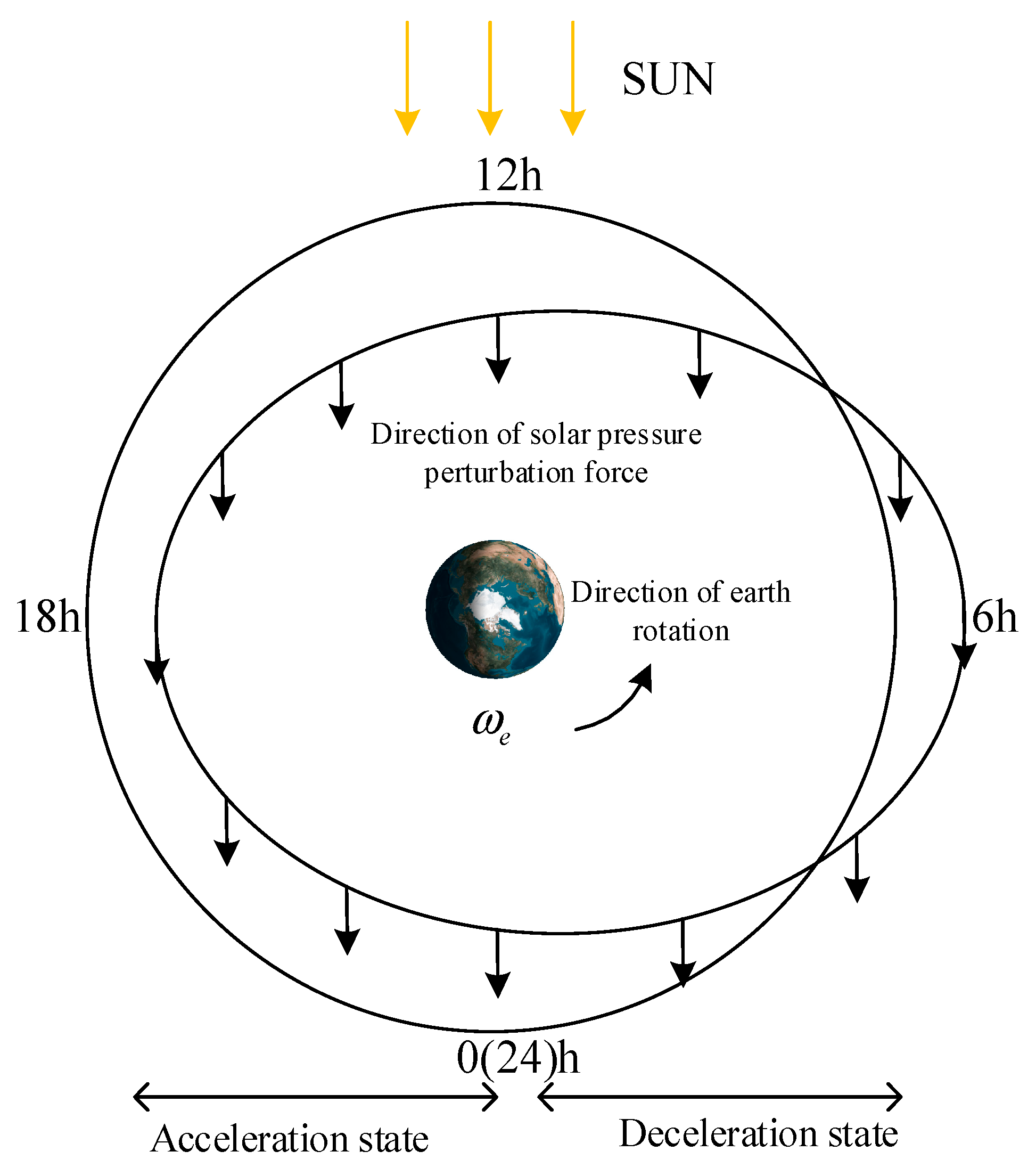
2.3.3. Solar Pressure Perturbation

The eccentricity of the GEO satellite under the influence of the solar pressure perturbation is as follows [34]:

$$\begin{array}{c}{\left(\frac{\mathrm{d}{e}_y}{\mathrm{d}t}\right)}_{\mathrm{P}}=-\sqrt{\frac{a_0}{\mu }}{C}_{\mathrm{R}}\left(\frac{S}{m}\right)P_0\left(-\frac{3}{2}{x}_{\mathrm{s}}+\frac{1}{2}{x}_{\mathrm{s}}\cos 2\lambda +\frac{1}{2}{y}_{\mathrm{s}}\sin 2\lambda \right)\\ {\left(\frac{\mathrm{d}{e}_x}{\mathrm{d}t}\right)}_{\mathrm{P}}=\sqrt{\frac{a_0}{\mu }}{C}_{\mathrm{R}}\left(\frac{S}{m}\right)P_0\left(-\frac{3}{2}{y}_{\mathrm{s}}+\frac{1}{2}{x}_{\mathrm{s}}\sin 2\lambda -\frac{1}{2}{y}_{\mathrm{s}}\cos 2\lambda \right)\end{array}$$

(20)

where

• Subscript “P” indicates the solar pressure perturbation term;
• $C_{\mathrm{R}}$ is the solar pressure coefficient, dimensionless;
• $S$ is the area of the satellite to the Sun, dimensionless;
• $P_0$ is the solar radiation pressure per square meter of sunlit area, dimensionless;
• $m$ is the mass of the satellite, in kg;
• $x_{\mathrm{s}}$ is the X-axis component of the center of mass of the Sun in the geocentric inertial frame (after normalization), in m;
• $y_{\mathrm{s}}$ is the Y-axis component of the center of mass of the Sun in the geocentric inertial frame (after normalization), in m;
• $z_{\mathrm{s}}$ is the Z-axis component of the center of mass of the Sun in the geocentric inertial frame (after normalization), in m;

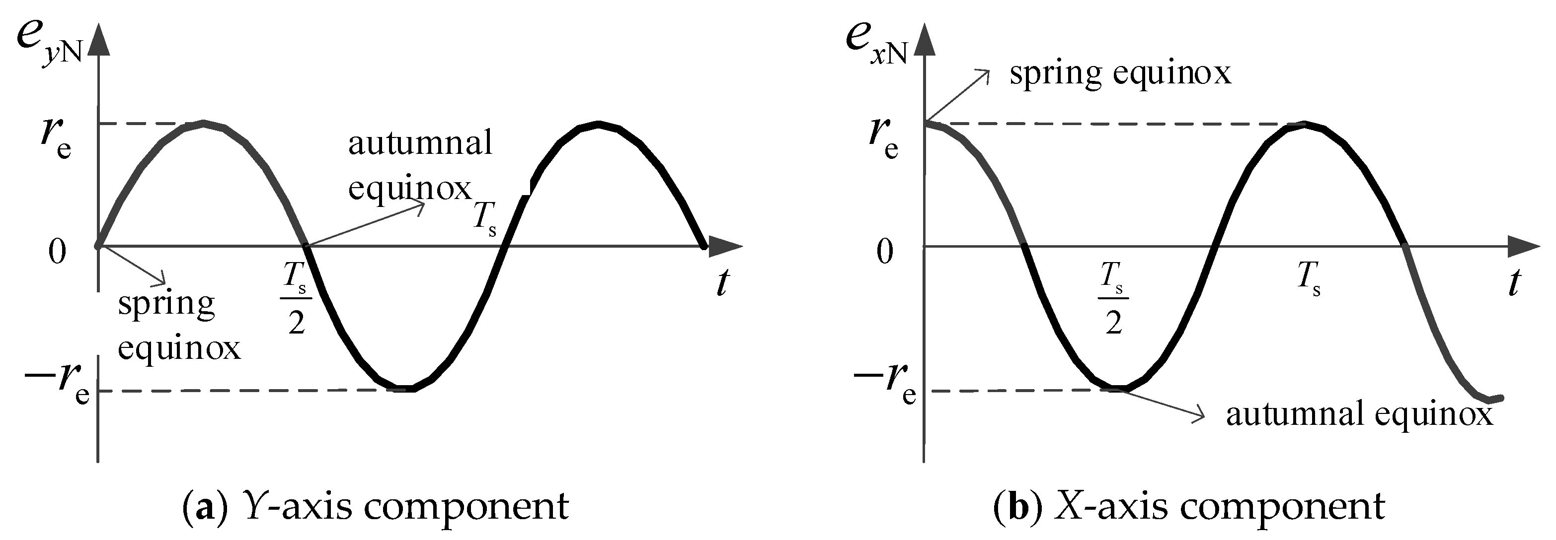
• From Formula (20), it can be obtained that the long period (annual period) motion of the eccentricity vector caused by the solar pressure perturbation is as follows:

$$\begin{array}{l}{\left(\frac{\mathrm{d}{e}_y}{\mathrm{d}t}\right)}_{\text{P-long}}=\frac{3}{2}\sqrt{\frac{a_0}{\mu }}{C}_{\mathrm{R}}\left(\frac{S}{m}\right)P_0{x}_{\mathrm{s}}\hfill \\ {\left(\frac{\mathrm{d}{e}_x}{\mathrm{d}t}\right)}_{\text{P-long}}=-\frac{3}{2}\sqrt{\frac{a_0}{\mu }}{C}_{\mathrm{R}}\left(\frac{S}{m}\right)P_0{y}_{\mathrm{s}}\hfill \end{array}$$

(21)

where subscript “P-long” indicates the long period (annual period) term of the solar pressure perturbation.

The long period oscillation of the eccentricity vector caused by the solar pressure perturbation is as follows:

$$\begin{array}{l}\mathrm{amp}{\left(e_y\right)}_{\text{P-long}}={\displaystyle \int {\left(\frac{\mathrm{d}{e}_y}{\mathrm{d}t}\right)}_{\text{P-long}}\mathrm{d}t}\\ \mathrm{amp}{\left(e_x\right)}_{\text{P-long}}={\displaystyle \int {\left(\frac{\mathrm{d}{e}_x}{\mathrm{d}t}\right)}_{\text{P-long}}\mathrm{d}t}\end{array}$$

(22)

Under the influence of solar light pressure perturbation, the eccentricity vector of the GEO satellite makes a circular motion with a period of years. Substituting Equation (21) into Equation (22), the radius of the circular motion can be obtained as follows:

$$R_{\mathrm{e}}=\frac{3}{2}\sqrt{\frac{a_0}{\mu }}{C}_{\mathrm{R}}\left(\frac{S}{m}\right)\frac{P_0}{{\omega }_{\mathrm{s}}}$$

(23)

According to Formula (23), when the reflection coefficient is 1.3 and the surface-to-mass ratio is 0.006 m²/kg, the radius of the circular motion of the eccentricity vector under the influence of sunlight pressure perturbation is about $R_{\mathrm{e}}=8.6\times {10}^{-5}$.

• From Formula (20), it can be obtained that the short period (diurnal period) motion of the eccentricity vector caused by the solar pressure perturbation is as follows:

$$\begin{array}{c}{\left(\frac{\mathrm{d}{e}_y}{\mathrm{d}t}\right)}_{\mathrm{P}}=-\sqrt{\frac{a_0}{\mu }}{C}_{\mathrm{R}}\left(\frac{S}{m}\right)P_0\left(\frac{1}{2}{x}_{\mathrm{s}}\cos 2\lambda +\frac{1}{2}{y}_{\mathrm{s}}\sin 2\lambda \right)\\ {\left(\frac{\mathrm{d}{e}_x}{\mathrm{d}t}\right)}_{\mathrm{P}}=\sqrt{\frac{a_0}{\mu }}{C}_{\mathrm{R}}\left(\frac{S}{m}\right)P_0\left(\frac{1}{2}{x}_{\mathrm{s}}\sin 2\lambda -\frac{1}{2}{y}_{\mathrm{s}}\cos 2\lambda \right)\end{array}$$

(24)

The short period oscillation of the eccentricity vector caused by the solar pressure perturbation is as follows:

$$\begin{array}{l}\mathrm{amp}{\left(e_y\right)}_{\text{P-short}}={\displaystyle \int {\left(\frac{\mathrm{d}{e}_y}{\mathrm{d}t}\right)}_{\text{P-short}}\mathrm{d}t}\\ \mathrm{amp}{\left(e_x\right)}_{\text{P-short}}={\displaystyle \int {\left(\frac{\mathrm{d}{e}_x}{\mathrm{d}t}\right)}_{\text{P-short}}\mathrm{d}t}\end{array}$$

(25)

where subscript “P-short” indicates the short period (diurnal period) term of the solar pressure perturbation.

According to Equation (25), the short period (diurnal period) oscillation amplitude of the eccentricity vector caused by the solar pressure perturbation is, approximately, as follows:

$$A_{\mathrm{pde}}=\frac{1}{4}\sqrt{\frac{a_0}{\mu }}{C}_{\mathrm{R}}\left(\frac{S}{m}\right)P_0\frac{1}{{\omega }_{\mathrm{e}}}$$

(26)

According to Formula (26), when the reflection coefficient is 1.3 and the surface-to-mass ratio is 0.006 m2/kg, the short period (diurnal period) oscillation amplitude of the GEO satellite eccentricity vector caused by the solar light pressure is about 10⁻⁸. The short period oscillation amplitude of the eccentricity vector caused by the solar light pressure is more than two orders of magnitude smaller than that caused by other gravitational perturbations. Therefore, the influence of sunlight pressure can be ignored when calculating the mean eccentricity vector.

In order to reduce unnecessary fuel consumption, the mean eccentricity only retains the annual periodic motion. Therefore, the calculation of the mean eccentricity vector needs to deduct not only the short period motion, but also the monthly oscillation caused by the lunar gravity. The perturbation forces that need to be deducted in the calculation of the mean eccentricity vector mainly include the Earth’s non-spherical gravitational perturbation, the diurnal period oscillation caused by the three-body gravitational perturbation, and the monthly period oscillation caused by the lunar gravitational perturbation. The mean eccentricity motion after deducting the corresponding period term is shown in Equation (27), as follows:

$$\begin{array}{l}\mathrm{amp}\left(e_y\right)=\mathrm{amp}{\left(e_y\right)}_{\text{E-short}}+\mathrm{amp}{\left(e_y\right)}_{\text{k-short}}+\mathrm{amp}{\left(e_y\right)}_{\text{m-long}}\\ \mathrm{amp}\left(e_x\right)=\mathrm{amp}{\left(e_x\right)}_{\text{E-short}}+\mathrm{amp}{\left(e_x\right)}_{\text{k-short}}+\mathrm{amp}{\left(e_x\right)}_{\text{m-long}}\end{array}$$

(27)

3. Eccentricity Keeping Method

The keeping of the relative fixed-point station of the GEO satellite can be regarded as the control of the orbit around the target satellite by a chief satellite [7,8]. The eccentricity will cause the longitude corresponding to the sub-satellite point of the satellite to fluctuate with the orbital period in the east–west direction near the position of the orbital mean longitude. The relationship between the fluctuation amplitude and the eccentricity is as follows:

$$\mathsf{\Delta }\lambda =2e$$

(28)

It can be seen from Equation (28) that the eccentricity will directly affect the accuracy of EWSK. To make the accuracy of EWSK meet the requirements, in addition to achieving the mean longitude keeping, it is also necessary to keep the eccentricity of the GEO satellite within an appropriate range.

It can be seen from Section 2.3 that the influence of solar light pressure on eccentricity is annual periodic and the diurnal periodic. The influence of the Moon’s gravity on the eccentricity is monthly periodic and diurnal periodic. The influence of the Earth’s non-spherical gravitational force on the eccentricity is diurnal periodic.

From the content of Section 2.3, it can be seen that the amplitude of the annual periodic oscillation of the eccentricity under the influence of perturbation is the largest, and it needs to be actively kept. On the other hand, the amplitude of monthly and diurnal periodic oscillations is small, and generally does not need to be actively kept. Because it is affected by the initial value of the eccentricity vector, the center of the circular motion of the eccentricity vector under the influence of sunlight pressure perturbation is not zero. This will cause large fluctuations in eccentricity, which in turn will cause large fluctuations in the east–west station of the satellite. Therefore, the eccentricity vector needs to be controlled within a certain range.

The annual periodic motion of the eccentricity vector is mainly affected by the sunlight pressure, and its principle is shown in Figure 1.

It can be seen from Figure 1 that when the GEO satellite is in the period from 12 to 24 o’clock local time, the satellite has been in the acceleration state. When the GEO satellite is in the period from 0 to 12 o’clock local time, the satellite has been in a state of deceleration. In a solar day, the satellite accelerates half of the time and decelerates half of the time. Therefore, the influence of the solar light pressure perturbation on the orbital semi-major axis can be considered to be zero, and the change direction of the eccentricity vector is 90° ahead of the orbital phase of the Sun. Since the period of the Sun’s motion around the Earth is one year, the motion period of the eccentricity vector under the influence of solar light pressure perturbation is also one year.

It can be seen from Equation (23) that when the reflection coefficient is 1.3 and the surface-to-mass ratio is 0.006 m²/kg, the radius of the circular motion of the eccentricity vector caused by the sunlight pressure is about $R_{\mathrm{e}}=8.6\times {10}^{-5}$. The efficiency for performing radial velocity increment on eccentricity is half of the tangential velocity increment. To obtain the maximum velocity increment envelope for eccentricity keeping, the maximum velocity increment for daily eccentricity vector keeping based on radial thrust is as follows:

$$v_{r\max }=\frac{2\pi \times 8.6\times {10}^{-5}{n}_0{a}_0}{365.25}\approx 0.0045\mathrm{m}/\mathrm{s}$$

(29)

3.1. Eccentricity Keeping Strategy

The mean longitude keeping zone is the same as the NSSK zone, and the SK zone is determined by the NSSK strategy. The SK zone cannot be adjusted according to the requirement of eccentricity keeping, so the tangential velocity increment for EWSK cannot be used to realize the active eccentricity keeping. In addition, the SK zone is relatively fixed in inertial space, and the required tangential velocity increments positioned at a geographic longitude increase linearly. Therefore, under the control of continuous mean longitude keeping, if the SK zone is not switched, the eccentricity vector will continue to diverge in one direction.

Although the eccentricity vector can be adjusted actively to a certain extent by deflecting the thrust direction slightly in the radial direction, the adjustment direction of the eccentricity vector is perpendicular to the direction of the increase in the eccentricity vector caused by the SK. Therefore, this method still cannot suppress the divergence trend of the eccentricity along the ±Y direction of the inertial frame.

In order to avoid the continuous divergence of the eccentricity vector, it is proposed that the satellite periodically alter its yaw direction to perform 180° maneuvers (that is, the satellite is switched between forward and backward flight), so that the NSSK zone is switched by 180°, meaning that the tangential velocity increment used for mean longitude keeping is not affected by the eccentricity. When the satellite is flying from the vernal equinox to the autumnal equinox, it is defined as the forward flight state of the satellite. At this time, the thruster direction points south (the velocity increment direction points north). When the satellite is flying from the autumnal equinox to the vernal equinox, it is defined as the backward flight state of the satellite. At this time, the thruster direction points north (the velocity increment direction points south). When the satellite passes through the vernal or autumn equinoxes, the yaw attitude of the satellite is maneuvered to 180° (that is, the satellite is switched forward/backward flight), which can prevent the divergence of the eccentricity vector during the keeping of the mean longitude. The increasing direction of the velocity vector is switched between the inertial system Y (backward flight) and the inertial system -Y (forward flight), which can avoid the unidirectional accumulation of the eccentricity vector caused by tangential orbital control at a fixed point for a long time. In theory, the higher the frequency of the satellite forward/backward flight switched, the higher the accuracy of eccentricity keeping.

The advantage of this method is that eccentricity keeping does not require fuel consumption. For GEO satellites, if the forward and backward flight switching is performed near the spring and autumn equinox, the satellite can also be fixed on the backlight surface, which is beneficial to the thermal control of the whole satellite and the layout of optical sensors. In addition, through the optimized design of the windsurfing drive shaft pointing, the angle between the normal of the windsurfing board and the direction of the Sun can be further reduced, which has a practical engineering application value. Therefore, this paper switches between forward and backward flight in the spring and autumn equinox. When the solar altitude angle of the ideal GEO orbit is positive, the satellite is in a forward flight state; on the contrary, when the solar altitude angle of the ideal GEO orbit is negative, the satellite is in a backward flight state.

At the spring and autumn equinox, the forward and backward flight switching is performed regularly and, theoretically, the eccentricity vectors accumulated in the Y and -Y directions of the inertial system can cancel each other out. The initial eccentricity vector error will cause the center of the eccentricity motion envelope to deviate from the center of the circle, and the peak value of the eccentricity magnitude is not minimum. In addition, due to the influence of the periodic term of the Earth’s nutation perturbation, the orbital inclination vector will fluctuate periodically [3], so the regular forward and backward flight switching will not cancel each other out of the eccentricity vectors generated by the mean longitude keeping but will instead have a small volume accumulation. To sum up, it is also necessary to centrally adjust the initial value of the eccentricity vector as needed. The specific adjustment principle is to use the radial velocity increment to make the current eccentricity vector return to the nominal state.

3.2. Eccentricity Vector in Uncontrolled State

According to the analysis in Section 2.3, under the action of perturbation, the eccentricity vector exhibits diurnal, monthly, and annual periodic fluctuations. The diurnal period fluctuation of the eccentricity vector caused by the non-spherical gravitation of the Earth, and the Sun–Moon gravitation is about $6.8\times {10}^{-5}$. The monthly period fluctuation of the eccentricity vector caused by the lunar gravity is about $3.7\times {10}^{-5}$; the annual period fluctuation of the eccentricity vector caused by the solar light pressure is about $8.6\times {10}^{-5}$. The fluctuation amplitudes of longitude caused by diurnal and monthly fluctuations are 0.008° and 0.002°, respectively. From the perspective of fuel saving, the diurnal and monthly fluctuations of eccentricity are generally not actively controlled. The eccentricity vector exhibits the characteristics of annual periodic circular variation, and the longitude fluctuation caused by it is about 0.005°. In order to minimize or even avoid eccentricity adjustment, it is generally suggested to place the circular motion center of the eccentricity vector at the center origin of the inertial system. In this way, the mean eccentricity vector always moves on a circle with zero as the center, the magnitude of the mean eccentricity is constant, and the eccentricity envelope is also the smallest.

From Equations (21) and (22), it can be obtained that the trajectory of the annual periodic motion of the uncontrolled mean eccentricity vector satisfies the following:

$$\begin{array}{l}{e}_{y\mathrm{N}}=e_{y\mathrm{N}0}+r_{\mathrm{e}}\sin {\lambda }_{\mathrm{s}}\\ e_{x\mathrm{N}}=e_{x\mathrm{N}0}+r_{\mathrm{e}}\cos {\lambda }_{\mathrm{s}}\end{array}$$

(30)

where $\left(e_{x\mathrm{N}0},e_{y\mathrm{N}0}\right)$ is the center of the annual periodic motion of the uncontrolled eccentricity vector, and ${\lambda }_{\mathrm{s}}$ is the solar right ascension starting from the inertial frame X.

By definition, the solar right ascension starting from the inertial frame X can be described as follows:

$${\lambda }_{\mathrm{s}}=n_{\mathrm{s}}{t}_{\mathrm{eL}}$$

(31)

where $t_{\mathrm{eL}}$ is the time length from the nearest vernal equinox, and its expression is as follows:

$$t_{\mathrm{eL}}=\mathrm{mod}\left(\left(jd-2451545\right)T_{\mathrm{d}},T_{\mathrm{s}}\right)$$

(32)

where $\mathrm{mod}\left(a,b\right)$ is the remainder of the number $a$ to the number $b$.

Substitute Equation (31) into Equation (30) to obtain the following:

$$\begin{array}{l}{e}_{y\mathrm{N}}=e_{y\mathrm{N}0}+R_{\mathrm{e}}\sin \left(n_{\mathrm{s}}{t}_{\mathrm{eL}}\right)\\ e_{x\mathrm{N}}=e_{x\mathrm{N}0}+R_{\mathrm{e}}\cos \left(n_{\mathrm{s}}{t}_{\mathrm{eL}}\right)\end{array}$$

(33)

It can be seen from Equation (30) that the change direction of the eccentricity vector is always perpendicular to the direction of the Sun, and the change direction of the eccentricity vector is 90° ahead of the orbital phase of the Sun, that is, the change direction of the eccentricity vector is the inertial system Z, and the Sun vector is the cross product.

From Formula (30), the uncontrolled eccentricity $e_{\mathrm{N}}$ can be obtained as follows:

$$e_{\mathrm{N}}=\sqrt{e_{y\mathrm{N}}{}^2+e_{x\mathrm{N}}{}^2}$$

(34)

To minimize the maximum value of $e_{\mathrm{N}}$, it must satisfy the following:

$$\begin{array}{l}{e}_{y\mathrm{N}0}=0\\ e_{x\mathrm{N}0}=0\end{array}$$

(35)

Substituting Equation (35) into Equation (33), the uncontrolled eccentricity vector that minimizes the maximum value of $e_{\mathrm{N}}$ is as follows:

$$\begin{array}{l}{e}_{y\mathrm{N}}=r_{\mathrm{e}}\sin \left(n_{\mathrm{s}}{t}_{\mathrm{eL}}\right)\\ e_{x\mathrm{N}}=r_{\mathrm{e}}\cos \left(n_{\mathrm{s}}{t}_{\mathrm{eL}}\right)\end{array}$$

(36)

According to Formula (36), the variation of the uncontrolled eccentricity vector is shown in Figure 2.

It can be seen that, if Formula (35) is satisfied, the eccentricity vector always points to the Sun. Therefore, the control strategy of making the eccentricity vector move in a circle with zero as the center is also called the “Sun-pointing” eccentricity keeping strategy.

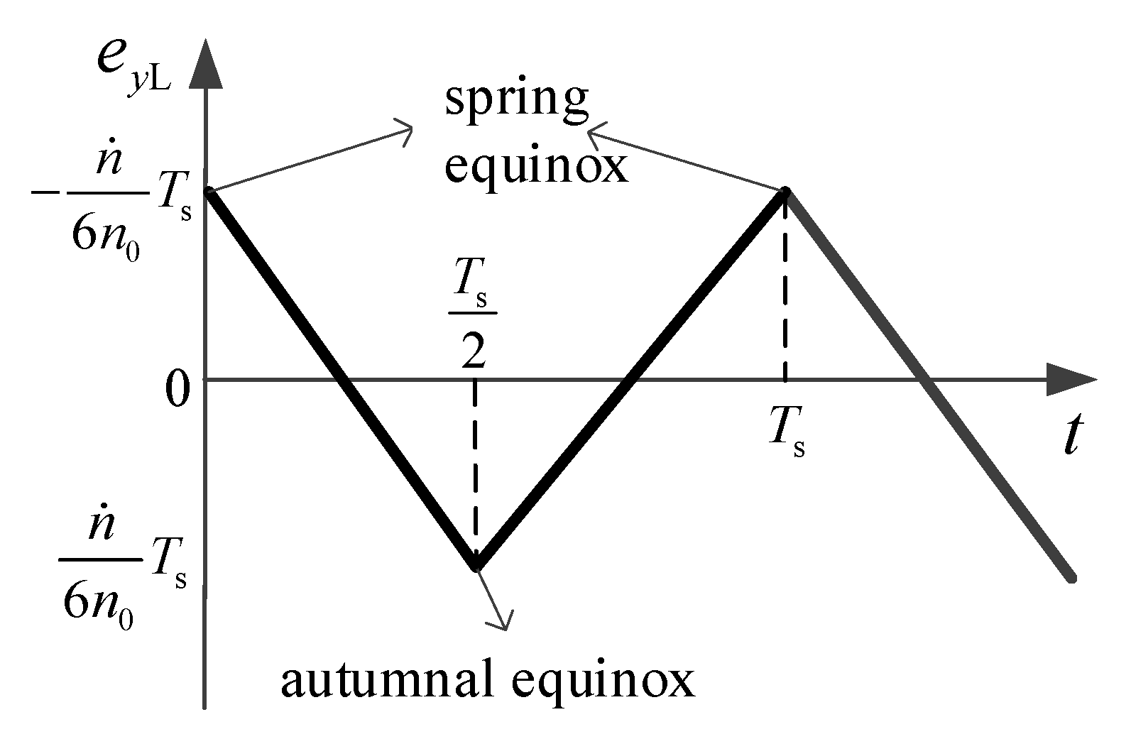
3.3. Eccentricity Vector under the Action of Mean Longitude Keeping

In addition to normal circular motion, the eccentricity vector also needs to superimpose the annual periodic motion caused by the mean longitude keeping. When the satellite is flying forward, the mean longitude keeping is performed in the normal direction of the SK zone, and the tangential velocity increment generated by the mean longitude keeping makes the eccentricity vector drift toward the mean inclination direction. When the satellite is flying backward, the mean longitude keeping is performed in the negative normal direction of the SK zone, and the tangential velocity increment generated by the mean longitude keeping causes the eccentricity vector to drift in the opposite direction of the mean inclination. In other words, the drift direction of the eccentricity vector and the drift direction of the inclination are in a straight line.

In order to minimize the orbital control amount caused by eccentricity fluctuation, it is hoped that the motion period of the mean inclination is greater than one year, and the larger the better. Therefore, it is a better choice to use the mean inclination under the influence of the Earth’s nutation period perturbation.

Reference [32] pointed out that the drift angle ${\theta }_{\mathsf{n}\mathsf{i}}$ of the mean inclination under the influence of the perturbation of the nutation period term is 18.6 years, and the fluctuation range is 81~99°. The drift angle ${\theta }_{\mathsf{n}\mathsf{i}}$ of the mean inclination vector can be considered as a constant value within one year, and the drift of the eccentricity vector caused by the velocity increment used for the mean longitude keeping can be regarded as a linear change, and its change rule is as follows:

$$\begin{array}{l}\mathsf{\Delta }{e}_{y\mathrm{L}}=-\mathrm{sign}\left(\beta \right)\frac{2\mathsf{\Delta }{\overline{v}}_t}{n_0{a}_0}\sin {\theta }_{\mathrm{ni}}\\ \mathsf{\Delta }{e}_{x\mathrm{L}}=-\mathrm{sign}\left(\beta \right)\frac{2\mathsf{\Delta }{\overline{v}}_t}{n_0{a}_0}\cos {\theta }_{\mathrm{ni}}\end{array}$$

(37)

where $\beta$ is the solar elevation angle of the ideal GEO orbit, that is, the solar elevation angle when the satellite inclination is zero, and its expression is follows:

$$\beta =\arcsin \left(z_{\mathrm{s}}\right)$$

(38)

In Formula (37), $\mathsf{\Delta }\overline{v}$ is the tangential velocity increment required for daily mean longitude keeping, and its expression is as follows:

$$\mathsf{\Delta }{\overline{v}}_t=\frac{a_0}{3}\dot{n}T$$

(39)

where $\dot{n}$ is the longitude drift angular acceleration of the satellite; $T$ is the nominal GEO satellite orbital period, equal to 1 mean sidereal day, about 86,164.091 s.

Integrating Equation (37), the change in eccentricity vector caused by the mean longitude keeping at any time can be obtained as follows:

$$\begin{array}{l}{e}_{y\mathrm{L}}=\{\begin{array}{cc}{e}_{y\mathrm{L}0}-\frac{2\dot{n}}{3n_0}{t}_{\mathrm{eL}}\sin {\theta }_{\mathsf{n}\mathsf{i}}& t_{\mathrm{eL}}\le \frac{T_{\mathrm{s}}}{2}\\ e_{y\mathrm{L}0}+\left(-\frac{2\dot{n}}{3n_0}\frac{T_{\mathrm{s}}}{2}+\frac{2\dot{n}}{3n_0}\left(t_{\mathrm{eL}}-\frac{T_{\mathrm{s}}}{2}\right)\right)\sin {\theta }_{\mathsf{n}\mathsf{i}}& t_{\mathrm{eL}}>\frac{T_{\mathrm{s}}}{2}\end{array}\\ e_{x\mathrm{L}}=\{\begin{array}{cc}{e}_{x\mathrm{L}0}-\frac{2\dot{n}}{3n_0}{t}_{\mathrm{eL}}\cos {\theta }_{\mathsf{n}\mathsf{i}}& t_{\mathrm{eL}}\le \frac{T_{\mathrm{s}}}{2}\\ e_{x\mathrm{L}0}+\left(-\frac{2\dot{n}}{3n_0}\frac{T_{\mathrm{s}}}{2}+\frac{2\dot{n}}{3n_0}\left(t_{\mathrm{eL}}-\frac{T_{\mathrm{s}}}{2}\right)\right)\cos {\theta }_{\mathsf{n}\mathsf{i}}& t_{\mathrm{eL}}>\frac{T_{\mathrm{s}}}{2}\end{array}\end{array}$$

(40)

where $\left(e_{x\mathrm{L}0},e_{y\mathrm{L}0}\right)$ is the initial value of the eccentricity vector caused by the mean longitude keeping; $T_{\mathrm{s}}$ is the rotation period of the Earth around the Sun, about 365.2425 mean solar days.

According to Formula (40), the magnitude of eccentricity caused by the mean longitude keeping can be obtained as follows:

$$e_{\mathrm{L}}=\sqrt{e_{y\mathrm{L}}{}^2+e_{x\mathrm{L}}{}^2}$$

(41)

To minimize the maximum value of $e_{\mathrm{L}}$, it must satisfy the following:

$$\begin{array}{l}{e}_{y\mathrm{L}}{}_{|t_{\mathrm{eL}}=T_{\mathrm{s}}/2}+e_{y\mathrm{L}}{}_{|t_{\mathrm{eL}}=0}=0\\ e_{x\mathrm{L}}{}_{|t_{\mathrm{eL}}=T_{\mathrm{s}}/2}+e_{x\mathrm{L}}{}_{|t_{\mathrm{eL}}=0}=0\end{array}$$

(42)

The above formula is simplified as follows:

$$\begin{array}{l}{e}_{y\mathrm{L}0}=\frac{\dot{n}}{6n_0}{T}_{\mathrm{s}}\sin {\theta }_{\mathsf{n}\mathsf{i}}\\ e_{x\mathrm{L}0}=\frac{\dot{n}}{6n_0}{T}_{\mathrm{s}}\cos {\theta }_{\mathsf{n}\mathsf{i}}\end{array}$$

(43)

Substituting Equation (43) into Equation (40), the eccentricity vector caused by mean longitude keeping at any time when the maximum value of $e_{\mathrm{L}}$ is minimized is as follows:

$$\begin{array}{l}{e}_{y\mathrm{L}}=\{\begin{array}{cc}\left(\frac{\dot{n}}{6n_0}{T}_{\mathrm{s}}-\frac{2\dot{n}}{3n_0}{t}_{\mathrm{eL}}\right)\sin {\theta }_{\mathsf{n}\mathsf{i}}& t_{\mathrm{eL}}\le \frac{T_{\mathrm{s}}}{2}\\ \left(-\frac{\dot{n}}{6n_0}{T}_{\mathrm{s}}+\frac{2\dot{n}}{3n_0}\left(t_{\mathrm{eL}}-\frac{T_{\mathrm{s}}}{2}\right)\right)\sin {\theta }_{\mathsf{n}\mathsf{i}}& t_{\mathrm{eL}}>\frac{T_{\mathrm{s}}}{2}\end{array}\\ e_{x\mathrm{L}}=\{\begin{array}{cc}\left(\frac{\dot{n}}{6n_0}{T}_{\mathrm{s}}-\frac{2\dot{n}}{3n_0}{t}_{\mathrm{eL}}\right)\cos {\theta }_{\mathsf{n}\mathsf{i}}& t_{\mathrm{eL}}\le \frac{T_{\mathrm{s}}}{2}\\ \left(-\frac{\dot{n}}{6n_0}{T}_{\mathrm{s}}+\frac{2\dot{n}}{3n_0}\left(t_{\mathrm{eL}}-\frac{T_{\mathrm{s}}}{2}\right)\right)\cos {\theta }_{\mathsf{n}\mathsf{i}}& t_{\mathrm{eL}}>\frac{T_{\mathrm{s}}}{2}\end{array}\end{array}$$

(44)

In Formula (44), due to $\sin {\theta }_{\mathsf{n}\mathsf{i}}\approx 1$, the variation in the eccentricity vector on the Y-axis component caused by the mean longitude keeping is shown in Figure 3.

It can be seen from Figure 3 that at the vernal equinox, the Y-axis component of the eccentricity vector caused by the mean longitude keeping is at its maximum. As the satellite switches from the backward flight state to the forward flight state, the Y-axis component of the eccentricity vector changes from linearly increasing to linearly decreasing. At the autumnal equinox, the Y-axis component of the eccentricity vector caused by the mean longitude keeping is minimum. As the satellite switches from the forward flight state to the backward flight state, the Y-axis component of the eccentricity vector changes from linearly decreasing to linearly increasing. At the summer and winter solstice, the eccentricity vector caused by the mean longitude keeping is zero.

In addition, the fluctuation amplitude of the Y-axis component of the eccentricity vector component caused by the mean longitude keeping is proportional to the magnitude of the acceleration of the mean longitude drift. When the geographic longitude of the fixed point is 121° east longitude, the fluctuation amplitude of X is the largest, about 0.00032.

3.4. Nominal Eccentricity Vector

In order to reduce fuel consumption, the eccentricity vector that fluctuates in diurnal and monthly periods is not actively kept. Select a reasonable initial value for the eccentricity vector with annual periodic fluctuations, try to use its own drift characteristics to make the eccentricity vector as small as possible, and only make small adjustments to the small amount of eccentricity vector deviation. In order to facilitate the real-time judgment of the eccentricity adjustment amount and the adjustment phase, it is necessary to calculate the current nominal eccentricity vector state in real-time.

The essence of eccentricity keeping is to adjust the mean eccentricity vector to the nominal eccentricity vector through control. When the mean eccentricity vector is in the nominal state, the motion envelope of the eccentricity vector is minimized through the combined effect of environmental perturbation and SK. Theoretically, the eccentricity vector can be kept without fuel consumption by this method.

From Section 2.2 and Section 2.3, it can be seen that the annual periodic motion of the uncontrolled eccentricity vector and the eccentricity vector caused by the mean longitude keeping is a circular motion with zero as the center. The eccentricity vector is uniquely determined, and both are only related to the Sun’s position, and the current nominal eccentricity vector can be uniquely determined only by the Sun’s position vector.

The nominal eccentricity vector $\left(e_{x\mathrm{NL}},e_{y\mathrm{NL}}\right)$ of the equivalent Sun-pointing is the superposition of the uncontrolled eccentricity vector and the eccentricity vector caused by the mean longitude. Combining Equations (36) and (44), the expression of $\left(e_{x\mathrm{NL}},e_{y\mathrm{NL}}\right)$ is as follows:

$$\begin{array}{l}{e}_{y\mathrm{NL}}=\{\begin{array}{cc}{R}_{\mathrm{e}}\sin \left(n_{\mathrm{s}}{t}_{\mathrm{eL}}\right)+\left(\frac{\dot{n}}{6n_0}{T}_{\mathrm{s}}-\frac{2\dot{n}}{3n_0}{t}_{\mathrm{eL}}\right)\sin {\theta }_{\mathsf{n}\mathsf{i}}& t_{\mathrm{eL}}\le \frac{T_{\mathrm{s}}}{2}\\ R_{\mathrm{e}}\sin \left(n_{\mathrm{s}}{t}_{\mathrm{eL}}\right)+\left(-\frac{\dot{n}}{6n_0}{T}_{\mathrm{s}}+\frac{2\dot{n}}{3n_0}\left(t_{\mathrm{eL}}-\frac{T_{\mathrm{s}}}{2}\right)\right)\sin {\theta }_{\mathsf{n}\mathsf{i}}& t_{\mathrm{eL}}>\frac{T_{\mathrm{s}}}{2}\end{array}\\ e_{x\mathrm{NL}}=\{\begin{array}{cc}{R}_{\mathrm{e}}\cos \left(n_{\mathrm{s}}{t}_{\mathrm{eL}}\right)+\left(\frac{\dot{n}}{6n_0}{T}_{\mathrm{s}}-\frac{2\dot{n}}{3n_0}{t}_{\mathrm{eL}}\right)\cos {\theta }_{\mathsf{n}\mathsf{i}}& t_{\mathrm{eL}}\le \frac{T_{\mathrm{s}}}{2}\\ R_{\mathrm{e}}\cos \left(n_{\mathrm{s}}{t}_{\mathrm{eL}}\right)+\left(-\frac{\dot{n}}{6n_0}{T}_{\mathrm{s}}+\frac{2\dot{n}}{3n_0}\left(t_{\mathrm{eL}}-\frac{T_{\mathrm{s}}}{2}\right)\right)\cos {\theta }_{\mathsf{n}\mathsf{i}}& t_{\mathrm{eL}}>\frac{T_{\mathrm{s}}}{2}\end{array}\end{array}$$

(45)

3.5. Eccentricity Adjustment Control Law

According to the difference between the current eccentricity vector and the nominal eccentricity vector, the control parameters for eccentricity adjustment at any time can be obtained.

The expression of the current mean eccentricity vector ${\overline{e}}_x,{\overline{e}}_y$ is as follows:

$$\begin{array}{l}{\overline{e}}_y=e_y-\mathrm{amp}\left(e_y\right)\\ {\overline{e}}_x=e_x-\mathrm{amp}\left(e_x\right)\end{array}$$

(46)

Let the eccentricity vector of the target satellite be the nominal eccentricity vector$e_{x\mathrm{NL}},e_{y\mathrm{NL}}$; then, the mean eccentricity vector $\delta {\overline{e}}_x,\delta {\overline{e}}_y$ of the chief satellite relative to the target satellite is as follows:

$$\begin{array}{l}\delta {\overline{e}}_y={\overline{e}}_y-e_{y\mathrm{NL}}\\ \delta {\overline{e}}_x={\overline{e}}_x-e_{x\mathrm{NL}}\end{array}$$

(47)

The impulse thrust control equation is as follows [34]:

$$\begin{array}{l}\mathsf{\Delta }{e}_y=-\frac{\mathsf{\Delta }{V}_{\mathrm{r}}}{V_{\mathrm{s}}}\cos \lambda +\frac{2\mathsf{\Delta }{V}_{\mathrm{t}}}{V_{\mathrm{s}}}\sin \lambda \\ \mathsf{\Delta }{e}_x=\frac{\mathsf{\Delta }{V}_{\mathrm{r}}}{V_{\mathrm{s}}}\sin \lambda +\frac{2\mathsf{\Delta }{V}_{\mathrm{t}}}{V_{\mathrm{s}}}\cos \lambda \end{array}$$

(48)

where

• $\mathsf{\Delta }{V}_{\mathrm{r}}$ is the radial velocity increment generated by orbital control;
• $\mathsf{\Delta }V$ is the tangential velocity increment generated by orbital control;
• $V_{\mathrm{s}}$ is the average linear velocity of the GEO satellite.

The eccentricity vector adjustment [36] using the tangential velocity increment will cause changes in both the mean longitude and the semi-major axis. Under the action of the normal mean longitude control, the tangential velocity increment generated by mean longitude keeping may weaken or offset the tangential velocity increment used to adjust the eccentricity vector. Therefore, the adjustment of the eccentricity vector must be performed with radial velocity increments.

From Equation (48), the radial velocity increment $\mathsf{\Delta }{V}_{\mathrm{r}}{}^{\mathrm{e}}$ used for the adjustment of the eccentricity vector is as follows:

$$\mathsf{\Delta }{V}_{\mathrm{r}}{}^{\mathrm{e}}=V_{\mathrm{s}}\sqrt{{\left({\overline{e}}_y-e_{y\mathrm{NL}}\right)}^2+{\left({\overline{e}}_x-e_{x\mathrm{NL}}\right)}^2}$$

(49)

From Formula (48), the orbital argument used for the eccentricity vector to centrally adjust the midpoint of the arc segment is as follows:

$${\lambda }^{\mathrm{e}}=\{\begin{array}{cc}\arctan \frac{e_{y\mathrm{NL}}-{\overline{e}}_y}{e_{x\mathrm{NL}}-{\overline{e}}_x}& {\overline{e}}_x-e_{x\mathrm{NL}}<0\\ \pi +\arctan \frac{e_{y\mathrm{NL}}-{\overline{e}}_y}{e_{x\mathrm{NL}}-{\overline{e}}_x}& {\overline{e}}_x-e_{x\mathrm{NL}}>0\\ \frac{\pi }{2}& {\overline{e}}_x-e_{x\mathrm{NL}}=0\&e_{y\mathrm{NL}}-{\overline{e}}_y>0\\ -\frac{\pi }{2}& {\overline{e}}_x-e_{x\mathrm{NL}}=0\&e_{y\mathrm{NL}}-{\overline{e}}_y<0\end{array}$$

(50)

where ${\lambda }^{\mathrm{e}}\in \left[-\pi /2,3\pi /2\right)$, and it needs to convert its range to $\left[-\pi ,\pi \right)$.

Eccentricity adjustment strategies can be divided into the following three types:

(1)

According to the control amount on the ground, to determine whether the eccentricity needs to be adjusted on the day;

(2)

According to the control amount, the satellite will automatically decide whether to perform an adjustment of the eccentricity on the day;

(3)

To perform eccentricity adjustment periodically (such as once a year) on the ground/on-satellite.

4. Simulation

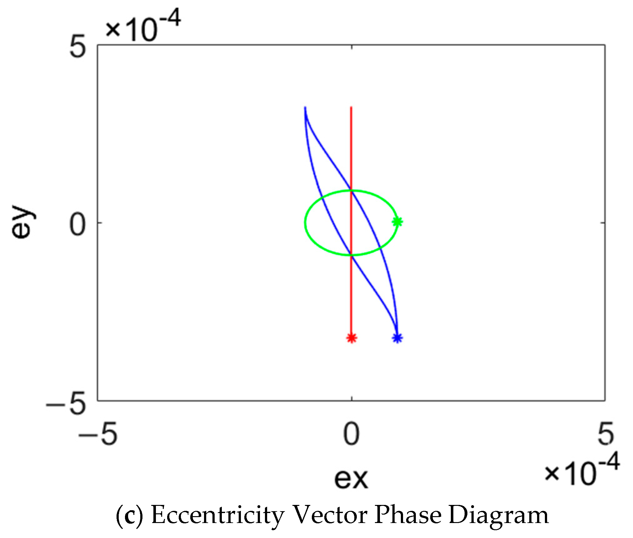
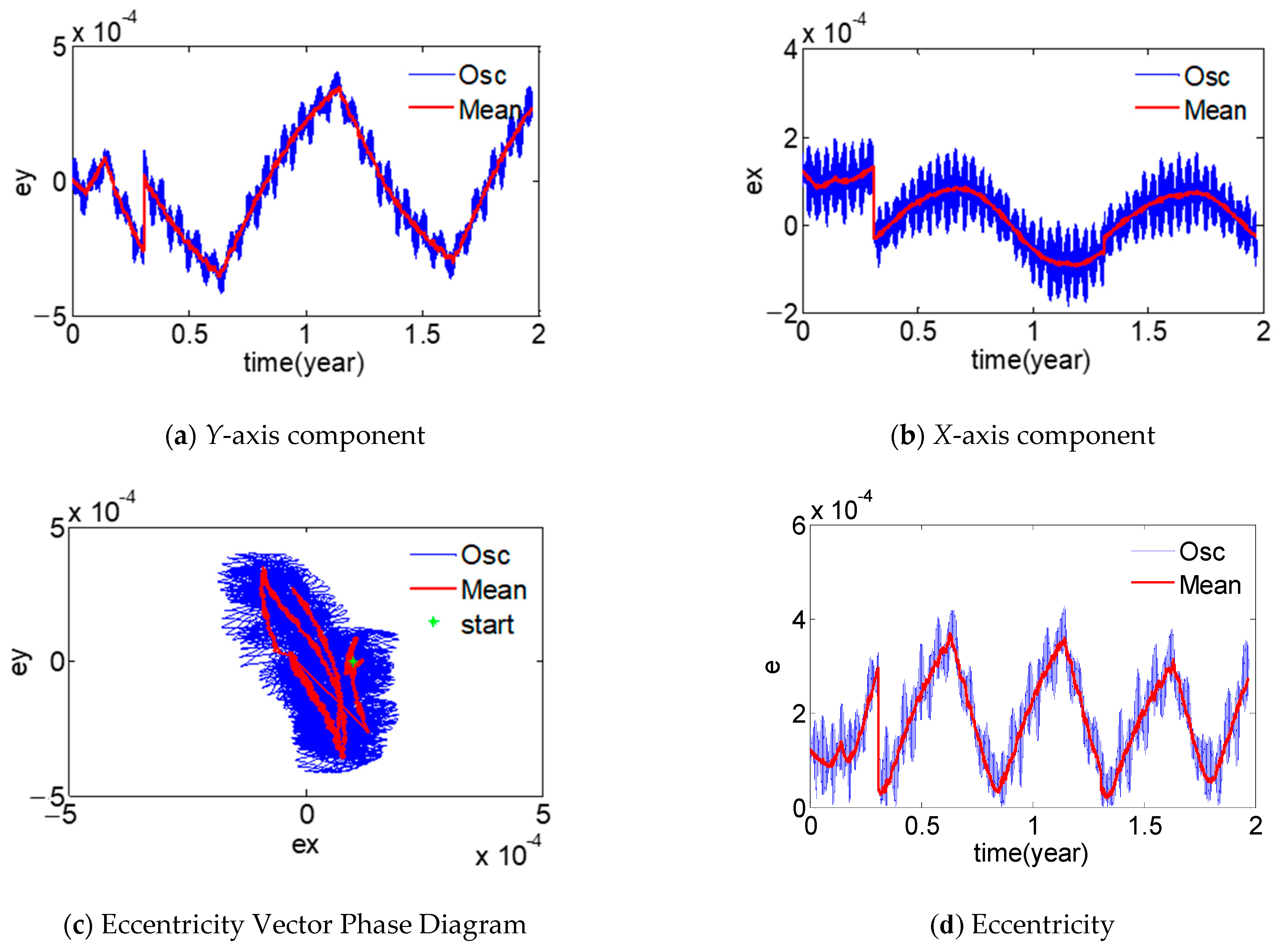
4.1. Eccentricity Vector Simulation

Taking 22 March 2025, 12:00 UTC as the time starting point, the reflection coefficient is 1.3, and the surface-to-mass ratio of the whole satellite is 0.006 m²/kg. The geographic longitude of the satellite location is 121° east longitude. Simulating a nutation period, the relationship among the uncontrolled eccentricity vectors, eccentricity vector under the action of mean longitude keeping, and the nominal eccentricity vector are shown in Figure 4.

In Figure 4, green line is the annual periodic drifting of the eccentricity under the influence of perturbation. Red line is the annual periodic drifting of the eccentricity under the longitude keeping control. Bule line is the annual periodic drifting of the eccentricity under the influence of perturbation and the control. It can be seen from Figure 4 that the uncontrolled eccentricity vector moves with the annual period. The eccentricity vector caused by the mean longitude keeping moves with the annual period and the nutation period. The nominal eccentricity vector is the superposition of the above two eccentricity vector, so the nominal eccentricity vector also moves with the annual period and the nutation period.

It can be seen from Figure 4 that the maximum value of the change envelope modulus of the nominal eccentricity vector under the influence of the perturbation of the nutation period term is 0.00036. The contribution of the mean eccentricity to the EWSK error under the influence of the perturbation of the nutation period term is less than 0.042°.

When considering the contribution of eccentricity to the EWSK error, it is also necessary to consider the influence of the short period terms, such as the diurnal and month of various perturbations on the eccentricity vector.

From the content of Section 2.3, it can be seen that the diurnal periodic oscillation amplitude of the eccentricity vector under the influence of the Earth’s non-spherical gravitational perturbation is $A_{\mathrm{ede}}=3.7\times {10}^{-5}$.The monthly periodic oscillation amplitude of the eccentricity vector under the influence of the lunar gravitational perturbation is $A_{\mathrm{mme}}=3.7\times {10}^{-5}$. The diurnal periodic oscillation amplitude of the eccentricity vector under the influence of the lunar gravitational perturbation is $A_{\mathrm{mde}}=1.4\times {10}^{-5}$. By superimposing the short period amplitudes of the above three items of eccentricity, the contribution of the mean eccentricity to the EWSK error is less than 0.01°.

In summary, using the eccentricity keeping strategy proposed in this paper, the contribution of eccentricity to the EWSK error is about 0.052°, which is suitable for the working condition where the EWSK accuracy is 0.1°.

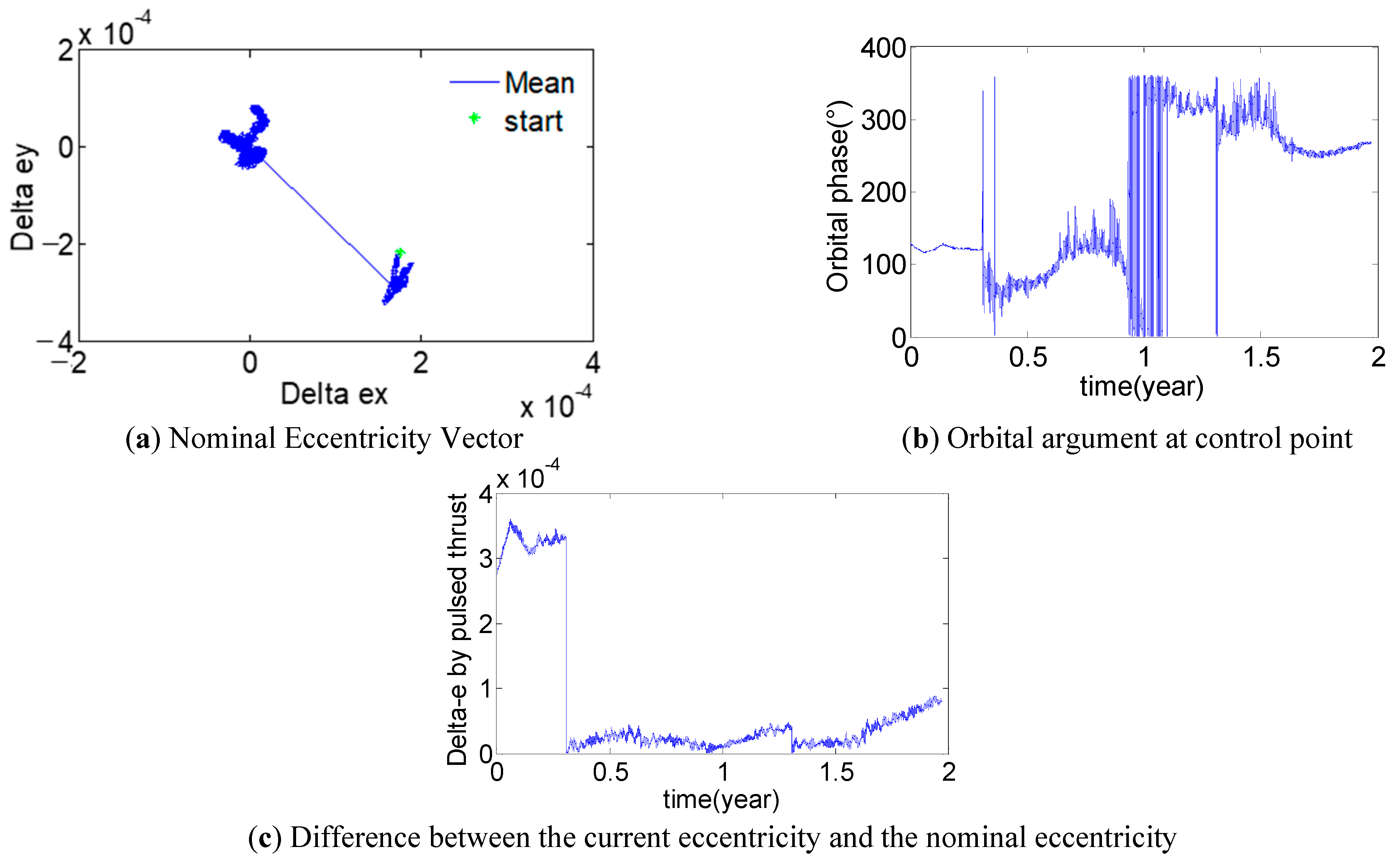
4.2. Eccentricity Control Simulation

The initial conditions of the simulation are shown in

Table 1. Initial orbit used for simulation.

Parameter	Value
Orbital start time $T_0$ (UTC)	2025-8-1 12:00:00
Orbital semi-major axis $a$ (km)	42166.300
Eccentricity $e$	0.0001
Inclination $i$ (°)	0.08
Argument of perigee $\omega$ (°)	0
Right ascending ascension node $\mathsf{\Omega }$ (°)	359.989
Mean anomaly $M$ (°)	251.361
Mean longitude $l$ (°)	121.019
Area of the satellite to the Sun $S$ (m2)	18
Satellite mass $m$ (kg)	3000
Solar pressure coefficient $C_{\mathrm{R}}$	1.3
Solar radiation pressure $P_0$ (N/m2)	4.56 × 10−6

. The eccentricity adjustment strategy is implemented periodically (one year). Without a loss of generality, the adjustment time of the eccentricity vector is 13:00 (UTC) on 22 November every year, and the fixed-point geographic longitude is 119°. The simulation time is 1800 days (about 5 years). After the adjustment, the mean eccentricity vector is shown in Figure 5.

It can be seen from Figure 5a–c that the eccentricity vector keeping is achieved. The actual eccentricity vector change curves are consistent with their corresponding theoretical curves in Figure 4a–c.

Comparing Figure 4a and Figure 5a, we can see that the actual mean eccentricity vector is slightly larger than the theoretical mean eccentricity vector. There are two reasons for this phenomenon. First, there exists an error in the process of the mean/osculating eccentricity vector switching; secondly, there exists an error in the eccentricity Sun-pointing model itself. Because in different years the control amounts of the NSSK and the EWSK are slightly different in different seasons, this will cause the movement trajectory of the eccentricity vector to present a non-closed feature, which needs to be eliminated through eccentricity adjustment.

The relevant control parameters of eccentricity adjustment are shown in Figure 6.

Figure 6a is the relative value of the current mean eccentricity vector and the nominal eccentricity vector. It can be seen that the mean eccentricity vector at the initial moment is far from the nominal eccentricity vector. After eccentricity is adjusted, the satellite’s mean eccentricity vector is controlled to the nominal eccentricity vector.

Figure 6b shows the orbital argument during the process of eccentricity adjustment. It can be seen that the initial mean eccentricity vector is far from the nominal eccentricity vector, and the orbital argument changes less, indicating that the phase of the orbital control is relatively fixed. After eccentricity adjustment, the fluctuation range of orbital argument is large, indicating that the orbital control phase is not fixed, and it also shows that the mean eccentricity vector and the nominal eccentricity vector coincide well.

Figure 6c is the difference between the current eccentricity and the nominal eccentricity. It can be seen that after the eccentricity adjustment, the difference between the current eccentricity and the nominal eccentricity is less than 0.0001.

5. Conclusions

Aiming at the problem that the eccentricity cannot be kept under the control strategy of inclination–longitude integrated keeping, a low fuel consumption keeping method of eccentricity under integrated keeping of inclination–mean longitude is proposed. According to the annual periodic motion characteristics of eccentricity under the action of perturbation, an eccentricity adjustment strategy is proposed. The annual velocity increment required for eccentricity adjustment is about 0.3 m/s, the eccentricity is controlled within the range of 0.0005, and the final EWSK accuracy is about 0.05°, which meets the requirement of GEO’s EWSK accuracy of 0.1°.

The eccentricity keeping method proposed in this paper can not only save the velocity increment required for SK, but can also reduce the number of SK times, simplify the SK process, and reduce the influence of SK interference on the whole satellite. This control method solves the problem that the eccentricity cannot be maintained under the control strategy of inclination–longitude integrated keeping. This method can be used for GEO satellites with long-term orbit keeping requirements, and can realize the long-term eccentricity keeping of GEO satellites with low fuel consumption. In addition, in the case of multiple thruster failure, the proposed method can achieve high precision eccentricity keeping with only one thruster.

In the future, the method of using one velocity increment to realize the integrated keeping of orbital inclination, longitude, and eccentricity can be considered, so as to further reduce the control frequency and fuel consumption and to increase the reliability of the satellite.

References

1. Chao, C.C. Applied Orbit Perturbation and Maintenance; The Aerospace Press: El Segundo, CA, USA, 2005. [Google Scholar]
2. Wang, Z.C.; Xing, G.H.; Zhang, H.W. Handbook of Geostationary Orbits; National Defense Industry Press: Beijing, China, 1999. [Google Scholar]
3. Zhang, N. High-Precision Positioning Technology for Geostationary Orbit Satellites. Ph.D. Thesis, Tsinghua University, Beijing, China, 2017. [Google Scholar]
4. Li, H.N. Geostationary Satellite Orbit and Co-Location Control Technology, 1st ed.; National Defense Industry Press: Beijing, China, 2010; pp. 61–64. [Google Scholar]
5. Li, H.N.; Gao, Y.J.; Yu, P.J. Research on GEO Co-location Control Strategy. Chin. J. Astronaut. 2009, 30, 967–973. [Google Scholar]
6. Park, B.K.; Tahk, M.J.; Bang, H.C.; Choi, S.B. Station Collocation Design algorithm for Multiple Geostationary Satellites Operation. J. Spacecr. Rockers 2003, 40, 889–893. [Google Scholar]
7. Li, J.C.; An, J.W. Co-location isolation strategy based on orbital eccentricity and orbital inclination vector square root. Spacecr. Eng. 2009, 18, 20–24. [Google Scholar]
8. Shi, S.B.; Dong, G.L.; Luo, Q. Orbit maintenance strategy for GEO co-located satellites based on isolation in the tangent plane. Shanghai Aerosp. 2009, 3, 47–55. [Google Scholar]
9. Shi, S.B.; Han, Q.L.; Lv, B.T. Optimal control of east-west orbit maintenance for GEO co-located satellites. Shanghai Aerosp. 2011, 2, 43–49. [Google Scholar]
10. Li, Y.H. Principles and Implementation Strategies of Orbit Maintenance for Geostationary Communication Satellites. J. Aircr. Meas. Control 2003, 22, 53–61. [Google Scholar]
11. Li, Y.H.; Wei, W.; Yi, K.C. Calculation and Engineering Implementation of Orbit Control Parameters of On-orbit Geostationary Satellites. Acta Space Sci. 2007, 27, 72–76. [Google Scholar]
12. Chen, Z.J.; Li, Y.H. Optimization method of east-west position keeping strategy for bias momentum satellites. Shanghai Aerosp. 2011, 28, 37–41. [Google Scholar]
13. No, T.S. Simple Approach to East-West Station Keeping of Geosynchronous spacecraft. J. Guid. Control Dyn. 1999, 22, 734–736. [Google Scholar] [CrossRef]
14. Yang, W.B.; Li, S.Y.; Li, N. Station-Keeping Control Method for GEO Satellite based on Relative Orbit Dynamics. In Proceedings of the 11th World Congress on Intelligent Control and Automation, Shenyang, China, 29 June–4 July 2014. [Google Scholar]
15. Yang, W.B.; Li, S.Y.; Li, N. Station-Keeping Control Method for High Orbit Spacecraft Based on Autonomous Control Architecture. In Proceedings of the 32nd Chinese Control Conference, Xi’an, China, 26–28 July 2013. [Google Scholar]
16. Vinod, K.; Hari, B.H. Autonomous Formation Keeping of Geostationary Satellites with Regional Navigation Satellites and Dynamics. J. Guid. Control Dyn. 2017, 40, 53–57. [Google Scholar]
17. Chang, J.S.; Li, Q.J.; Yuan, Y. East-west position keeping strategy of continuous equally spaced pulse thrust for geostationary satellites. Space Control Technol. Appl. 2013, 39, 24–32. [Google Scholar]
18. Possner, M.P.; Almendra, M.; Garcia, G. A New Flight Dynamics Solution for Operations of the Boeing 702 Satellite. In Proceedings of the AIAA Space 2008 Conference & Exposition, San Diego, CA, USA, 9–11 September 2008. [Google Scholar]
19. Feuerborn, S.A.; Neary, D.A.; Perkins, J.M. Finding a way: Boeing’s All Elecric Propulsion Satellite. In Proceedings of the 49th AIAA/ASME/SAE/ASEE Joint Propulsion Conference, San Jose, CA, USA, 14–17 July 2013. [Google Scholar]
20. Weiss, A.; Cairano, D. Station Keeping and Momentum Management of Low-thrust Satellites Using MPC. Aerosp. Sci. Technol. 2018, 76, 229–241. [Google Scholar] [CrossRef]
21. Lin, S.Y.; Li, M.; Yang, Z. Position maintenance and momentum wheel unloading control of electric propulsion satellites based on model prediction and orbit recursion. In Proceedings of the 4th Annual Conference on High Resolution Earth Observation, Wuhan, China, 17–18 September 2017. [Google Scholar]
22. Caverly, R.; Cairano, D.; Weiss, A. Split-Horizon MPC for Coupled Station Keeping, Attitude Control, and Momentum Management of GEO Satellites using ElectricPropulsion. In Proceedings of the 2018 Annual American Control Conference (ACC), Milwaukee, WI, USA, 27–29 June 2018. [Google Scholar]
23. Weiss, A.; Kalabic, U.; Cairano, S. Model Predictive Control for Simultaneous Station keeping and Momentum Management of Low-thrust Satellites. In Proceedings of the 2015 American Control Conference (ACC), Chicago, IL, USA, 1–3 July 2015. [Google Scholar]
24. Walsh, A.; Cairano, D.; Weiss, A. MPC for coupled station keeping, attitude control, and momentum management of low-thrust geostationary satellites. In Proceedings of the 2016 Annual American Control Conference (ACC), Boston, MA, USA, 6–8 July 2016. [Google Scholar]
25. Frederik, J.; Bruijn, D. Geostationary Satellite Station-Keeping Using Convex Optimization. J. Guid. Control Dyn. 2015, 39, 605–616. [Google Scholar]
26. Gazzino, C.; Arzelier, D.; Cerri, L.; Losa, D.; Louembet, C.; Pittet, C. A Three-step Decomposition Method for Solving the Minimum-fuel Geostationary Station Keeping of Satellites Equipped with Electric Propulsion. Acta Astronatica 2019, 158, 12–22. [Google Scholar] [CrossRef] [Green Version]
27. Gazzino, C.; Arzelier, D.; Losa, D.; Louembet, C.; Pittet, C.; Cerri, L. Optimal Control for Minimum-fuel Geostationary Station Keeping of Satellites Equipped with Electric Propulsion. IFAC Pap. Online 2016, 49, 379–384. [Google Scholar] [CrossRef]
28. Gazzino, C.; Louembet, C.; Arzelier, D.; Jozefowiez, N.; Losa, D.; Pittet, C.; Cerri, L. Interger Programming for Optimal Control of Geostationary Station Keeping of Low-thrust Satellites. In Proceedings of the 20th IFAC World Congress 2017, Toulouse, France, 9–14 July 2017. [Google Scholar]
29. Gazzino, C.; Arzelier, D.; Louembet, C.; Cerri, L.; Pittet, C.; Losa, D. Long-Term Electric-Propulsion Geostationary Station-Keeping via Integer Programming. J. Guid. Control Dyn. 2019, 42, 976–991. [Google Scholar] [CrossRef]
30. Sukhanov, A.A.; Prado, A.F. On one Approach to the Optimization of Low-thrust Station Keeping Manoeuvres. Adv. Space Res. 2012, 50, 1478–1488. [Google Scholar] [CrossRef]
31. Roth, M. Strategies for Geostationary Spacecraft Orbit SK Using Electrical Propulsion Only. Ph.D. Thesis, Czech Technical University, Prague, Czech Republic, 2020. [Google Scholar]
32. Ye, L.; Liu, C.; Zhu, W.; Yin, H.; Liu, F.; Baoyin, H. North/south Station Keeping of the GEO Satellites in Asymmetric Configuration by Electric Propulsion with Manipulator. Mathematics 2022, 10, 2340. [Google Scholar] [CrossRef]
33. Liu, F.; Ye, L.; Liu, C.; Wang, J.; Yin, H. Micro-thrust, Low-fuel Consumption, and High-precision East/west Station Keeping for GEO Satellites based on Synovial Variable Structure Control. Mathematics 2023, 11, 705. [Google Scholar] [CrossRef]
34. Kuai, Z. Z Research on GEO Satellite Orbit Maintenance and Orbit Transfer Strategy under Pulse and EP. Ph.D. Thesis, University of Science and Technology of China, Hefei, China, 2017. [Google Scholar]
35. Ye, L.; Wang, J.; Baoyin, H. Constellation maintenance and capture of sun-synchronous frozen orbits. Space Control Technol. Appl. 2021, 47, 24–32. [Google Scholar]
36. Yin, J.; He, Q.; Han, C. Collision analysis of spacecraft relative motion based on relative orbital elements. J. Aeronaut. Astronaut. 2011, 32, 311–320. [Google Scholar]
Figure 1. Schematic diagram of the influence of solar light pressure perturbation on the eccentricity vector of GEO satellites (viewed from the Earth’s North Pole).
Aerospace 10 00135 g001
Figure 2. Uncontrolled eccentricity vector.
Aerospace 10 00135 g002
Figure 3. The eccentricity vector on the Y-axis component caused by the mean longitude keeping.
Aerospace 10 00135 g003
Figure 4. Mean eccentricity vector in one nutation period.
Aerospace 10 00135 g004aAerospace 10 00135 g004b
Figure 5. Result of eccentricity vector adjustment.
Aerospace 10 00135 g005
Figure 6. Control parameters for eccentricity adjustment.
Aerospace 10 00135 g006