Influence of the Reynolds Number on the Aerodynamic Performance of a Small Rotor

Abstract

The use of small rotors has increased due their applications in drones and UAVs. In order to improve the global performance of these aerial vehicles, it is necessary to understand the aerodynamics of small rotors, since this is related to the global energy consumption of such vehicles. Most of the computational fluid dynamics (CFD) studies found in the literature that are related to the analysis of small rotors employ fully turbulent models, despite the low-to-moderate Reynolds numbers of these applications. This paper presents CFD simulations for a small rotor at hover at different Reynolds numbers using fully turbulent and transitional SST $k-\omega$ turbulence models. Numerical results show that thrust and torque are close to experimental measurements, showing differences of less than 5% for both fully turbulent and transitional models. However, significant differences were observed between the fully turbulent and the transitional models when studying the boundary-layer development and separation. As the Reynolds number was increased, it was observed that at the tip of the blade, these differences were reduced, but at mid-span, the differences were more obvious.

1. Introduction

The use of unmanned aerial vehicles (UAVs) and drones has increased in the last few years, especially those that are capable of vertical take-off and landing (VTOL). The preferred platform for this type of aerial vehicle is the multicopter (in particular, the quadcopter), which uses rotors as the propulsion system due to their high maneuverability and VTOL characteristics. The flow field developed by a rotor operating at hover is complex and impacts the aerodynamic performance. Therefore, understanding the flow developed at hover when the rotor operates at low to moderate Reynolds numbers ($Re$) is important for the design of vehicles of this type. There are different approaches to studying the aerodynamics of rotors: theoretical approximations, experimental studies, and computational simulations. As stated by Ramasamy M., Jhonson B., and Leishman J. [1], the theory developed for the analysis of full-scale rotors is not suited to the analysis of small-scale rotors due flow simplifications considered for high $Re$. Experimental methods can become highly expensive, especially when the study of additional aerodynamics features (besides thrust and torque) is included. Computational simulations can be used as an alternative approach to the study of the aerodynamics of rotors and can provide information about those aerodynamic features that is difficult to observe and quantify from basic experiments.

Among the different computational methods employed in the study of rotors aerodynamics, CFD simulations are highly used and preferred. Some studies on full-scale rotors have found inaccuracies of CFD results using Reynolds-Averaged Navier–Stokes (RANS) solvers. Duraisamy and Baeder [2] used a high-resolution RANS solver to investigate the evolution of tip vortices of rotary blades. They observed numerical diffusion because of inaccuracies of the discretization of the convective term in the Navier–Stokes equations and inaccurate turbulence modeling due to an imperfect closure model in the RANS equations. However, reliable solutions can be obtained from a simple rotational correction to the production term. A similar conclusion was achieved by Postdam and Pulliam [3], who investigated the influence of turbulence models for the vertical wake of a rotorcraft. They performed CFD simulations using the Spalart–Allmaras and $k-\omega$ SST turbulence models. Problems were found with the dependence of the vorticity on the eddy-viscosity production term. Results were improved using curvature corrections or by turning off production terms. Regarding small-scale rotors, Gomez S. et al. [4] analyzed the effects that a bio-inspired rotor blade shape have on the size and structure of a tip vortex. An SST version of the $k-\omega$ turbulence model was used with curvature correction. Results of the bio-inspired blade were compared to those found when using a rectangular blade, demonstrating advantages of the bio-inspired blade, as the vortex size and strength are reduced at the tip of the blade. Liu and Luo [5] conducted CFD simulations of a 9 inch in diameter rotor using the Spalart–Allmaras turbulence model and a sliding-mesh technique. Simulations were performed for hovering and forward-flight conditions. The differences between the numerical results for thrust and power coefficients and experimental data were less than 3%. Kutty H. and Parvathy R. used CFD simulations to study the performance of a 254 mm rotor at different advance ratios [6]. They used the multi-reference frame method with an unstructured grid. The $k-ϵ$, $k-\omega$, and SST $k-\omega$ turbulence models were used. It was found that results from the $k-\omega$ model were closer to experimental data from the literature. However, there was over-prediction of the power coefficient for a high advance ratio and an under-prediction for a low advance ratio. Rovere et al. [7] used unsteady RANS simulations, overset grids, and the SST $k-\omega$ turbulence model to study the performance of small rotors operating with out and in-ground effects. Experimental results from Ramasamy M., Jhonson B., and Leishman J. [1] were used to validate computational results. Experiments were performed for rotors of 86 mm with different blade shapes. Thrust and torque computational results were in agreement with experiments, though outflow differences were found in the far wake. Argus F. et al. [8] studied the disturbance-amplification factor required to induce a laminar–turbulent transition in a $0.508$ m in radius rotor. They used a mid-fidelity solver where a RANS model was coupled with a blade element momentum theory model. Results for hover simulations were compared with experimental measurements. It was found that operating conditions such as rotor vibrations, aeroelastic effects, and surface roughness affect the performance of the rotors. In addition, laminar separation of the boundary layer led to a strong fall in the hover rotor efficiency. However, if the transition from a laminar to turbulent boundary layer was developed without separation, the boundary layer was thinner and there was less reduction in the lift. Henricks. et al. [9] conducted a computational study to understand the effects that twist, taper, and pitch have on the aerodynamic performance of a small hovering rotor. Different designs were evaluated for a rotor with a radius of $188.65$ mm operating at 4000 RPM, while keeping the airfoil constant. CFD simulations were executed using the detached eddy simulation (DES) turbulence model. It was established that twist and taper improved the aerodynamic performance of the rotor; higher pitch increases the thrust coefficient more significantly than twist, and taper decreases it. It was shown that even for the highest pitch tested, there was no flow separation, which enhanced the aerodynamics and noise reduction. Serre R. et al. [10] investigated how some flow features, for example, flow separation, impact the noise generated by a small rotor. To study the flow separation, they used experimental measurements for oil-flow visualization and high-fidelity, computational lattice Boltzmann methods using large eddy simulations. The mesh consisted of $249\times {10}^6$ cells with a $y^{+}$ of 50 on the tip. For the boundary-layer separation, it was found that separation occurs at the leading edge, and a second separation zone was identified at the trailing edge. These experimental observations agree with computational results. It was also observed that the separation at the leading edge could enhance the noise generated from these rotors. Garofano-Soldado A. at.al. [11] studied the ground effect on small-scale tilted rotors using experiments and CFD simulations. Three different rotors were used with diameters from 9 to 18 inches and Reynolds numbers from $0.46\times {10}^5$ to $2.2\times {10}^5$. The computational method used the multiple reference frame approximation, the SST $k-\omega$ turbulence model, and an unstructured grid of $3.5\times {10}^6$ elements with a $Y^{+}$ of 31. The computational results agreed well with the experiments, and it was demonstrated that a steady-state approximation can capture the aerodynamics of the rotor while grounded.

Computational studies performed on small-scale rotors proved that RANS approximations can provide adequate results for the thrust and torque developed by these rotors. Most of these studies used a fully turbulent model even when the operational $Re$ of these rotors suggested that they are not the best-suited models. In addition, those studies present results for the velocity field, pressure, and vorticity, yet information on parameters such as induced velocity and the boundary layer has caught less attention. Small-scale rotors are used in the development of unmanned multicopters. These vehicles are suited for complex tasks from topographic studies to Martian missions. However, the aerodynamics of these rotors is not fully understood, and important features such as the boundary layer, separations zones, and rotor response at atypical air conditions need to be investigated.

The present paper shows and discusses simulations of a small rotor at hover with different $Re$ through a CFD model which includes an unstructured grid and a steady-state approach. The model was implemented in the commercial CFD software ANSYS FLUENT v17.0. In addition, two RANS based approximations were used: a fully turbulent and a transition-turbulence model, both of them based on the SST $k-\omega$ model. Thrust and torque computational results were compared with experimental measurements that were performed at three different altitudes in Colombia.

This paper presents the responses of a small rotor operating at a variety of air conditions which affect the performance of such rotors. Due to the complex design of these rotors, zones with a thick laminar boundary layer are developed; therefore, improvements in the design of these zones can lead to the development of thinner boundary layers, or even a quick transition to a turbulent boundary layer, which can improve the performance. This study shows that the use of a transition-turbulence model instead of a fully turbulent model could lead to a better understanding of the rotor aerodynamics. In addition, it is shown that the use of a transition-turbulence model not only allows one to study of the developed boundary layer, but also leads to better predictions of torque and thrust, and predicts some flow features that are not captured with a fully turbulent model.

2. Methodology

2.1. Experimental

2.1.1. Setup and Sensors

The primary objectives of the experiments that were performed were to measure the thrust and torque developed by the rotor, each as a function of its angular velocity, and to characterize the aerodynamic hover performance of a motor–rotor system. Figure 1 shows a simplified scheme of the experimental setup used to test the motor–rotor system. Samples of thrust, torque, and angular velocity can be taken and measured simultaneously. The electrical power of the motor was delivered by a variable DC voltage source (reference 257 2260B-80-27 from the manufacturer Keithley), and it was set to 14 V. To control the angular velocity of the motor, a pulse width modulation (PWM) signal was generated using a “Pololu Micro-Maestro” servo controller card. The frequency of the PWM was set to 50 Hz, and the pulse width was varied from $1.2$ to $1.6$ ms. The Pololu card was connected to the computer through a USB port, and its output was connected to the electronic speed controller (ESC). The ESC was a SimonK Firmware Multicopter Speed Controller (SK-20A) with a maximum operating current of 20 A and an operational voltage input from 6 to $16.8$$V_{DC}$. The thrust was measured with a load-cell-type donut, model LTH300, from the manufacturer FUTEK. Torque was measured using a reaction torque sensor, model TFF400, from the same manufacturer. The angular velocity was measured with a phototransistor reflection sensor, model E3FB Retro-Reflective (OMROM). All the sensors were energized with a variable power supply, model PS280 (Tektronix), which was set to 18 $V_{DC}$. Torque, thrust, and angular velocity measurements are acquired with a NI-9205 module, with a sample rate of 1000 Hz.

2.1.2. Experiments

Experiments attempted to characterize the thrust and torque developed by the rotor at different angular velocities. However, controlling the angular velocity of the rotor is a difficult task due to the variations in the air conditions at different altitudes. These variations cause the motor–rotor to develop different velocities for the same PWM signal, so to reach the same velocity, fine adjustments of the PWM were necessary. This was a complex control scenario; therefore, it was decided to use the PWM wide pulse as the control variable. Five levels of the PWM wide pulse were selected (duty cycles of: 6.4%, 6.9%, 7.2%, 7.5%, and 7.9%). These PWM duty cycles were selected because they corresponded to angular velocities of the motor without load of 3000, 4005, 4497, 5001, and 5502 RPM. For each angular velocity, the rotor operated for 60 seconds in order to reach a steady state. Thrust, torque, and rotational velocity data were acquired for 30 s. Then, the PWM signal was set to the next level and the process was repeated.

The experiments were performed in three different locations in Colombia: Bogota (2600 m.a.s.l), Bucaramanga (900 m.a.s.l), and Cartagena (2 m.a.s.l). For each test, the temperature (T), atmospheric pressure ($P_r$), and relative humidity ($RH$) at the site of the experiment were measured. During the tests, the variations in the measured variables were lower than $0.1\%$; hence, they were not taken into consideration. With the averaged air properties that were measured, air density was estimated using Equation (1) (see reference [12]:

$$\rho =\frac{P_r{M}_a}{ZRT}(1-0.378x_v),$$

(1)

where $M_a$ is the molar mass of dry air, Z is the compressibility factor, R is the molar gas constant, and $x_v$ is the mole fraction of water vapor. The air viscosity was calculated using Sutherland’s equation:

$$\mu ={\mu }_0\left(\frac{T_0+C_S}{T+C_S}\right){\left(\frac{T}{T_0}\right)}^{\frac{3}{2}},$$

(2)

where $\mu$ is the viscosity in centipoise at temperature T in Kelvin, ${\mu }_0=0.1827$ is the reference viscosity in centipoise at reference temperature $T_0=291$ K, and $C_S=120$ is Sutherland’s constant.

Table 1. Air properties for the different locations.

Location	${\mathit{P}}_{\mathit{r}}$ (Pa)	T (°C)	RH (%)	$\mathit{\rho }$ (kg/m3)	$\mathit{\mu }$ (Pa·s)
Bogota	74,500	19.7	53	0.89	$1.84\times {10}^{-5}$
Bucaramanga	90,600	26.7	50	1.06	$1.87\times {10}^{-5}$
Cartagena	101,400	24.6	64	1.19	$1.86\times {10}^{-5}$

summarizes the air properties at the different locations in which the experiments were performed.

The rotor Reynolds number defined by Equation (3) was varied between $4\times {10}^4$ and $1\times {10}^5$ in the tests that were performed. In the definition of rotor $Re$, R is the rotor radius, w is the angular velocity, and C is the chord length at $75\%$ of the span of the rotor.

$$Re=\frac{\rho \left(0.75R\right)wC}{\mu }$$

(3)

2.2. Computational

2.2.1. Models

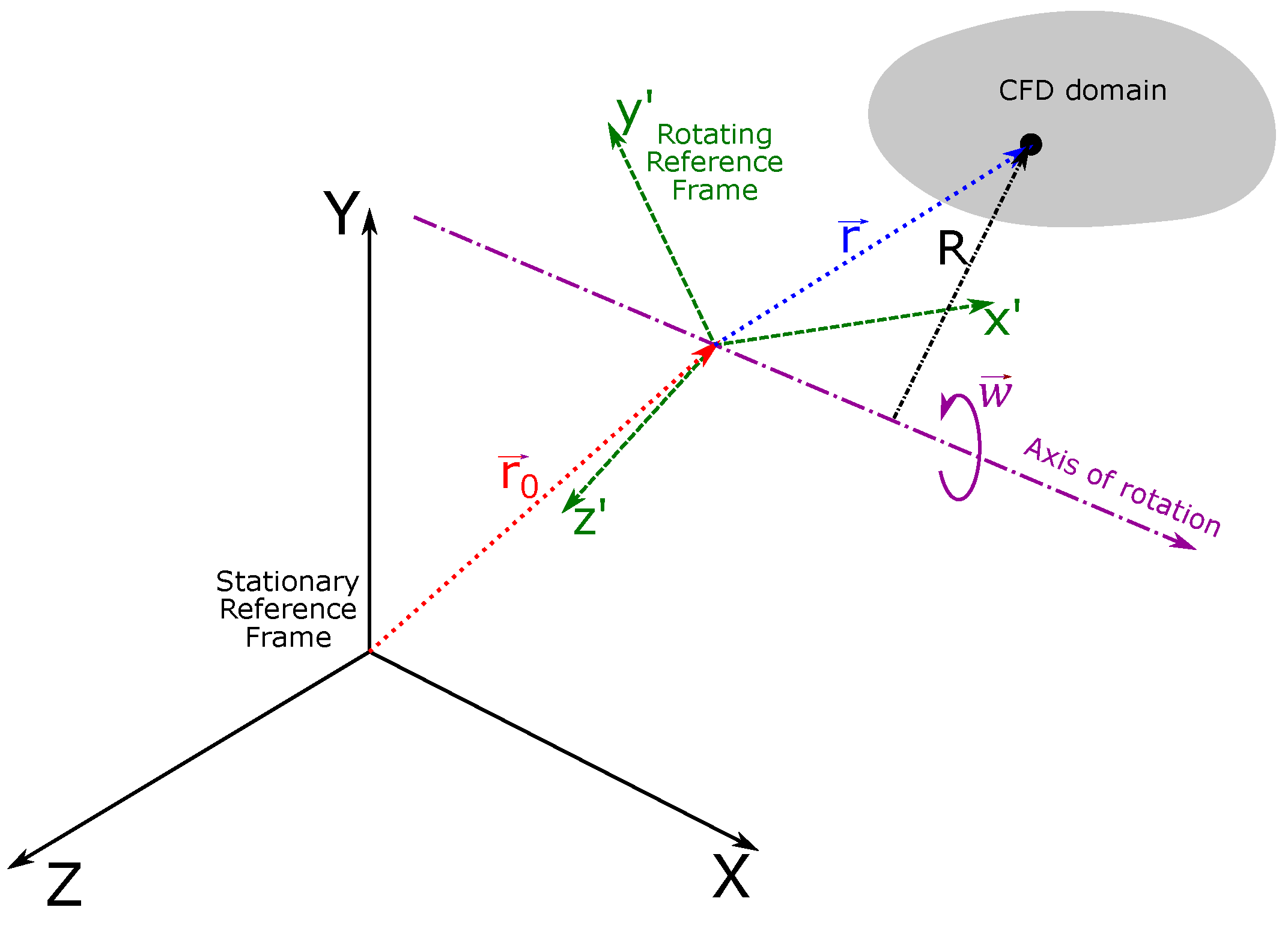
The nature of the flow generated by a rotating rotor in hover is unsteady; this implies that for a simulation of this problem, a dynamic mesh method is typically required. If computational resources are limited, remeshing, sliding, and overset mesh methods are not suitable for these kinds of simulations. In addition, the rotational speeds of rotors used in drones can be as high as 5000 RPM, which would require very a small time step for a full transient simulation. An alternative to overcome these difficulties is to study the problem with a moving reference frame attached to the rotor in which the flow can be modeled as a steady-state. For this, a multiple reference frame (MRF) technique is used, and in some cases, the whole domain can be reduced to a single reference frame (SRF) [13]. In this method, the moving reference frame rotates with a constant angular velocity ($\overrightarrow{\omega }$) with respect to a stationary reference frame. The computational domain is defined with respect to the rotational reference frame, and any point, a position can be expressed by a vector $\overrightarrow{r}$ from this reference frame, as shown by Figure 2.

Velocities can be transformed from the stationary reference frame to the rotating reference frame using Equation (4):

$${\overrightarrow{v}}_r=\overrightarrow{v}-\overrightarrow{\omega }\times \overrightarrow{r},$$

(4)

where ${\overrightarrow{v}}_r$ is the velocity measured from the rotating reference frame, and $\overrightarrow{v}$ is the velocity measured from the stationary reference frame.

In this reference frame, the governing equations (i.e., Reynolds-Averaged Navier–Stokes (RANS) equations) are modified to include new acceleration terms. These equations can be expressed using absolute averaged velocities, so that Equations (5) and (6) represent mass and momentum conservation for a steady and incompressible flow. The Coriolis and centripetal accelerations are expressed by $\left(\overrightarrow{\omega }\times \overrightarrow{v}\right)$, $\nu$ represents the kinematic viscosity, and $\overline{\overline{\tau }}$ represents the Reynolds stress tensor:

$$\nabla ·{\overrightarrow{v}}_r=0,$$

(5)

$$\nabla ·\left({\overrightarrow{v}}_r\overrightarrow{v}\right)+\left(\overrightarrow{\omega }\times \overrightarrow{v}\right)=-\nabla \left(\frac{p}{\rho }\right)+\nu {\nabla }^2\overrightarrow{v}+\nabla ·\overline{\overline{\tau }}$$

(6)

Different turbulence models have been used to simulate the flow around a rotor at hover. The shear-stress transport (SST) version of the $k-\omega$ turbulence model was developed to have a strong and accurate formulation of the $k-\omega$ turbulence model near the wall and the free-stream independence of the $k-ϵ$ model in the far field. The refinements in this formulation are:

• a blending function was designed to activate the $k-\omega$ model in the region near to the wall and to activate the $k-ϵ$ model away from the surface;
• the turbulent viscosity definition was modified to account for the transport of the turbulent shear stress;

With these refinements, the model is more reliable for a wider class of flows, such as those with adverse pressure gradients, airflows, and transonic shock waves. In the case of rotating flows, such as those developed by rotors, the $k-\omega$ SST turbulence model requires modification to the production terms. This modification allows the model to have better performance in flows with rotation and strong curvature in the streamlines. Postdam and Pulliam [3] and Duraisamy and Baeder [2] have found that results of rotor simulations are improved if the turbulence models are used with curvature correction. Details of the $k-\omega$ SST and SST-CC (curvature correction) models can be found in references [14,15]. Another important element in the correct selection of a turbulence model in the present application is that small rotors used on quadcopters usually operate at low to moderate $Re$, typically lower than $1\times {10}^5$. Therefore, it is more adequate to use a transition model to study the flow developed by these types of rotors. The transition SST $k-\omega$ model is based on the coupling of the SST $k-\omega$ with an equation for intermittency and one for the transition criteria, in terms of momentum thickness Reynolds number ${\widetilde{Re}}_{\theta t}$. This turbulence model (including curvature correction) was used in the present work, and it has four differential equations. This implies a higher computational cost that is compensated for with the use of an SRF. More information on the SST $k-\omega$ transitional model can be found in reference [16].

2.2.2. Simulation Setup

The object of study of this research was a commercial rotor made of fiber carbon that is typically used in small to medium drones and quadcopters (see Figure 3). The rotor diameter (D) is 360 mm, the chord at the root is $20.77$ mm, the tip chord is $4.33$ mm, and the chord at $75\%$ of the span is $25.31$ mm. The rotor’s CAD model was obtained by a 3D scanning using a NextEngine Scanner with an accuracy of $0.05$ mm. This is the same rotor used in references [17,18].

The computational domain is a vertical cylinder, with a diameter of $1.2$ m ($3.3$D) and a length of $2.5$ m (7D); the rotational axis of the rotor is aligned with the axis of the cylinder and at $0.97$ m ($2.7$D) from the upper surface of the cylinder. These dimensions were evaluated using simulation results of torque and thrust at several rotational velocities. First, the diameter of the computational domain was varied from $1.2$ to $2.2$ m. It was found that differences in thrust were less than $0.6\%$, and for torque the maximum difference was lower than $1.9\%$. When the length downstream the rotor was increased from $1.5$ to $2.5$ m, differences in torque and thrust predictions were less than $2.0\%$. These results indicate that an increase in $83\%$, of the computational domain diameter, does not have a significant impact on the simulation results. If the length upstream the rotor was increased by $67\%$, its effect on the simulations was negligible. Boundary conditions were set as pressure inlet for the cylinder’s upper and lateral surfaces; at the lower surface a pressure outlet was set, and the rotor’s wall was adjusted as a non-slip wall. Figure 4 shows the computational domain and its boundary conditions.

The mesh was generated with the ANSYS Meshing software. An unstructured mesh that consists of tetrahedral elements with a refinement of pyramidal elements near the rotor’s wall was generated. The grid-convergence study was performed using the fully turbulent $k-\omega$ SST model in five different meshes while varying the number of elements (from $8.0\times {10}^6$ to $16.5\times {10}^6$) and using torque and thrust results at 5221 RPM (the experimental velocity at which the maximum thrust was achieved in Bogota) as convergence criteria. It was observed that an increase in the number of elements from $9.2\times {10}^6$ to $16.5\times {10}^6$ represents differences of $0.2\%$ and $0.03\%$ in the thrust and torque predictions, respectively. Therefore, a mesh with approximately $9\times {10}^6$ cells was selected. More details of the computational domain, boundary conditions, and mesh can be found in references [17,18].

All simulations were implemented in the commercial CFD software ANSYS FLUENT v17.0. The pressure–velocity coupling solver SIMPLE was used, second-order upwind discretizations were used for convective terms, the least squares cell scheme was used for the gradients, and PRESTO was the pressure interpolation scheme. Convergence criteria were set to $1\times {10}^{-6}$, and all the simulations were run until convergence criteria were reached or residuals reached a steady value lower than $1\times {10}^{-3}$.

2.2.3. Cases

For this computational study, 20 different air conditions were considered based on varying the density ($0.867$–$1.173$ kg/m³) and the viscosity ($1.795\times {10}^{-5}$–$1.931\times {10}^{-5}$ Pa·s). These variations were selected with a Sobol sequence based on the conditions of the physical experiments. For each of these air conditions, simulations were performed by increasing the rotational velocity with small discrete steps, starting with 1 RPM angular velocity and ending up with 6500 RPM; 24 discrete steps were necessary for both turbulence models that were used (SST $k-\omega$ and transition SST $k-\omega$). This means that for each turbulence model, approximately 480 computational cases were run while varying the rotor’s Reynolds number (see Equation (3) between $3\times {10}^4$ and $2\times {10}^5$. All simulations in this study were performed at the cluster “Magnus” of Universidad de los Andes, using 32 processors, Intel X86_64, capable of 2.4 GHz, and 64 GB RAM. For the fully turbulent model, each simulation took 20 h approximately, whereas for the transitional turbulence model, this time was increased to $23.5$ h.

3. Results

3.1. Validation

Computational results based on global rotor performance parameters and based only on the SST $k-\omega$ turbulence model were compared against experimental data for validation purposes. The performance parameters used were thrust and torque coefficients, which are defined by Equations (7) and (9):

$$C_T=\frac{T_r}{\rho A{\left(wR\right)}^2},$$

(7)

$$C_Q=\frac{Q}{\rho AR{\left(wR\right)}^2},$$

(8)

where $T_r$ is the thrust, Q is the torque, and A is the area of the rotor, i.e., $\pi R^2$. Thrust and torque coefficients of the simulations that used $Re$ close to the experimental ones are summarized in

Table 2. Experimental and computational thrust and torque coefficients.

	Experimental		Computational
Re	$C_T$	$C_Q$	Re	$C_T$	$C_Q$
$4.86\times {10}^4$	$1.052\times {10}^{-2}$	$1.431\times {10}^{-3}$	$4.74\times {10}^4$	$1.056\times {10}^{-2}$	$1.412\times {10}^{-3}$
$5.87\times {10}^4$	$1.054\times {10}^{-2}$	$1.406\times {10}^{-3}$	$5.92\times {10}^4$	$1.072\times {10}^{-2}$	$1.419\times {10}^{-3}$
$6.87\times {10}^4$	$1.035\times {10}^{-2}$	$1.407\times {10}^{-3}$	$7.05\times {10}^4$	$1.084\times {10}^{-2}$	$1.424\times {10}^{-3}$
$7.87\times {10}^4$	$1.053\times {10}^{-2}$	$1.424\times {10}^{-3}$	$7.91\times {10}^4$	$1.091\times {10}^{-2}$	$1.425\times {10}^{-3}$
$9.82\times {10}^4$	$1.122\times {10}^{-2}$	$1.444\times {10}^{-3}$	$9.87\times {10}^4$	$1.098\times {10}^{-2}$	$1.428\times {10}^{-3}$

. All the experimental uncertainties in $C_T$ and $C_Q$ were less than 6.5% (see Appendix A). $Re$ variation between experiments and simulations is explained by the fact that in the experiments the control variable was the PWM; therefore, the velocity developed by the rotor–motor system did not match with the velocities adjusted for the simulations. It is possible to observe that thrust coefficient values predicted with the simulations are slightly higher than the experimental measurements.

It is clear that CFD predictions for torque coefficient were closer to experimental measurements than thrust coefficient predictions. Further, CFD results are within the uncertainty values of the experimental measurements; the highest difference between experiments and simulations for the thrust coefficient was $4.7\%$, and for torque, it was $1.3\%$.

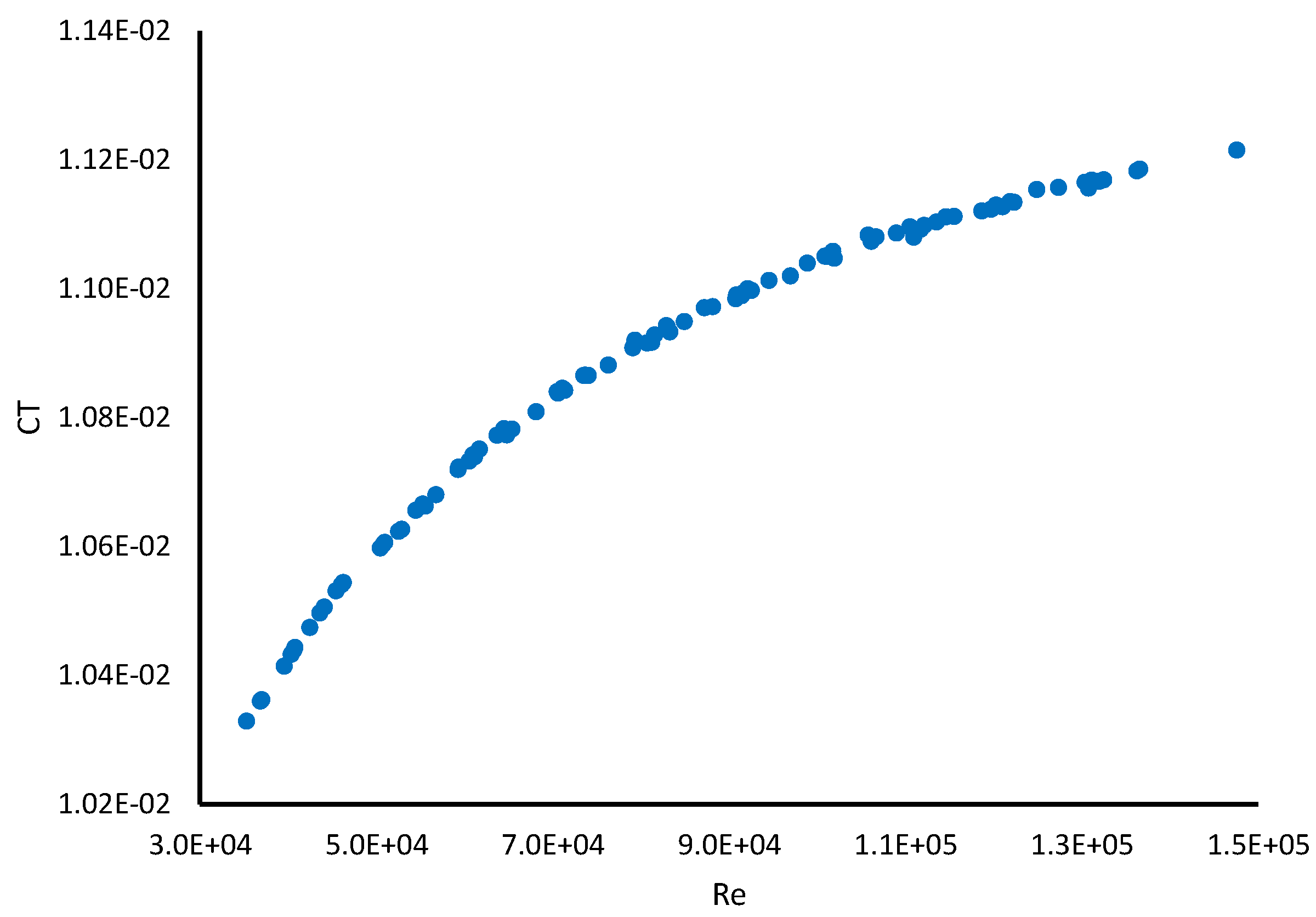
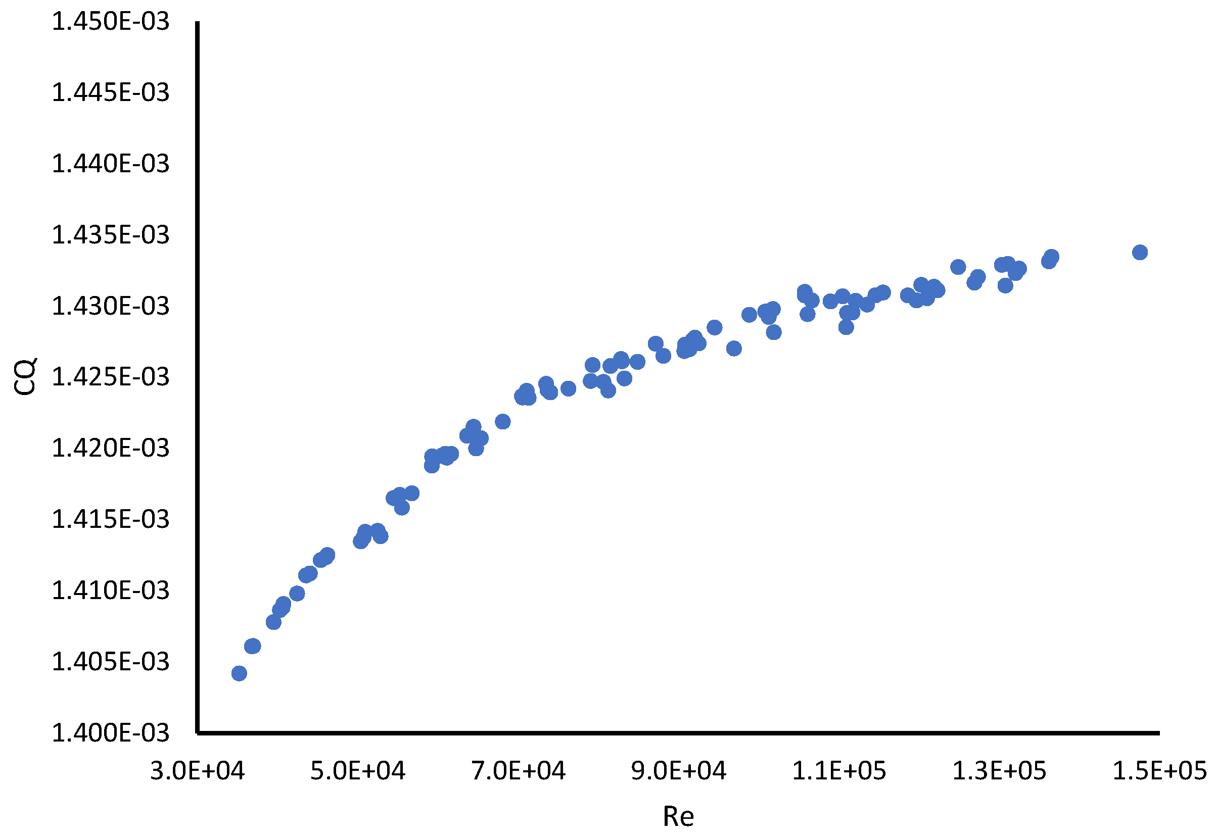
In the experiments, it was not possible to reach a $Re$ higher than $1.0\times {10}^5$, but through simulations, it was possible to explore the behavior of the rotor at higher operational Reynolds numbers. This evaluation was achieved with the results of the simulation cases explained in Section 2.2.3. In these computational simulations, $Re$ was varied from $3.53\times {10}^4$ up to $1.48\times {10}^5$. Figure 5 presents the values of thrust coefficient starting at $1.033\times {10}^{-4}$ and a apparent asymptotic tendency to a value of $1.125\times {10}^{-2}$. It is observed that the torque coefficient develops a minimum value of $1.404\times {10}^{-3}$ and has a noticeable tendency to a value of $1.435\times {10}^{-3}$, as shown by Figure 6. For the range of $Re$ studied, the thrust coefficient grew by $8.6\%$, and for the torque coefficient there was an increment of $2.1\%$. It is clear that the aerodynamic performance of the rotor depends on the operational $Re$.

3.2. Turbulence Models Comparison

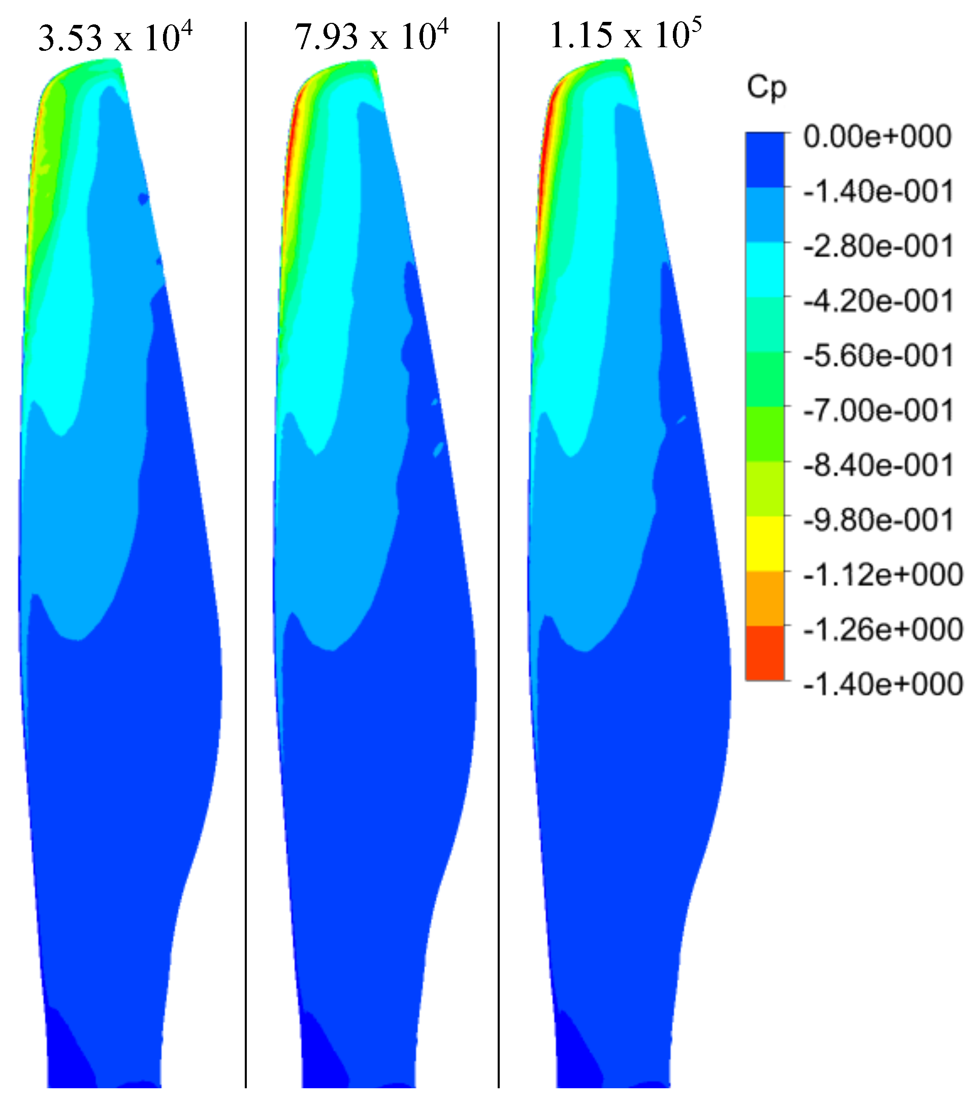
As was shown in the previous section, the simulations covered a wide range of Reynolds numbers; therefore, only simulations at 2000, 4500, and 6500 RPM were chosen to compare the turbulence models that were used. For these angular velocities, the Reynolds numbers were, respectively: $3.53\times {10}^4$, $7.93\times {10}^4$, and $1.15\times {10}^5$. The comparison between the turbulence models was performed based on the performance prediction (thrust and torque), pressure distribution, and separation prediction along the rotor blade.

3.2.1. Thrust and Torque

Table 3. Thrust and torque coefficients for fully turbulent and ransition-turbulence models.

	Transition		Fully Turbulent
Re	$C_T$	$C_Q$	$C_T$	$C_Q$
$3.53\times {10}^4$	$1.033\times {10}^{-2}$	$1.404\times {10}^{-3}$	$1.027\times {10}^{-2}$	$1.387\times {10}^{-3}$
$7.93\times {10}^4$	$1.092\times {10}^{-2}$	$1.426\times {10}^{-3}$	$1.103\times {10}^{-2}$	$1.432\times {10}^{-3}$
$1.15\times {10}^5$	$1.111\times {10}^{-2}$	$1.431\times {10}^{-3}$	$1.118\times {10}^{-2}$	$1.442\times {10}^{-3}$

summarizes thrust and torque coefficient results for fully turbulent and transition-turbulence models. It is clear that both turbulence models predict similar values for thrust and torque with differences of less than $1.25\%$ between them. The closest experimental result (see Table 2) was when $Re=7.87\times {10}^4$ with a $C_T=1.053\times {10}^{-2}$ and $C_Q=1.424\times {10}^{-2}$; it is observed that the transitional turbulence model predicted closer values at a $Re=7.93\times {10}^4$ for both thrust and torque with differences of less than 3%.

3.2.2. Pressure Distribution

The pressure coefficient $\left(C_P\right)$ was used to compare the pressure field over the rotor among the turbulence models at different rotational velocities. This coefficient was estimated using Equation (9):

$$C_P=\frac{P-P_{ref}}{0.5\rho {V_{ref}}^2},$$

(9)

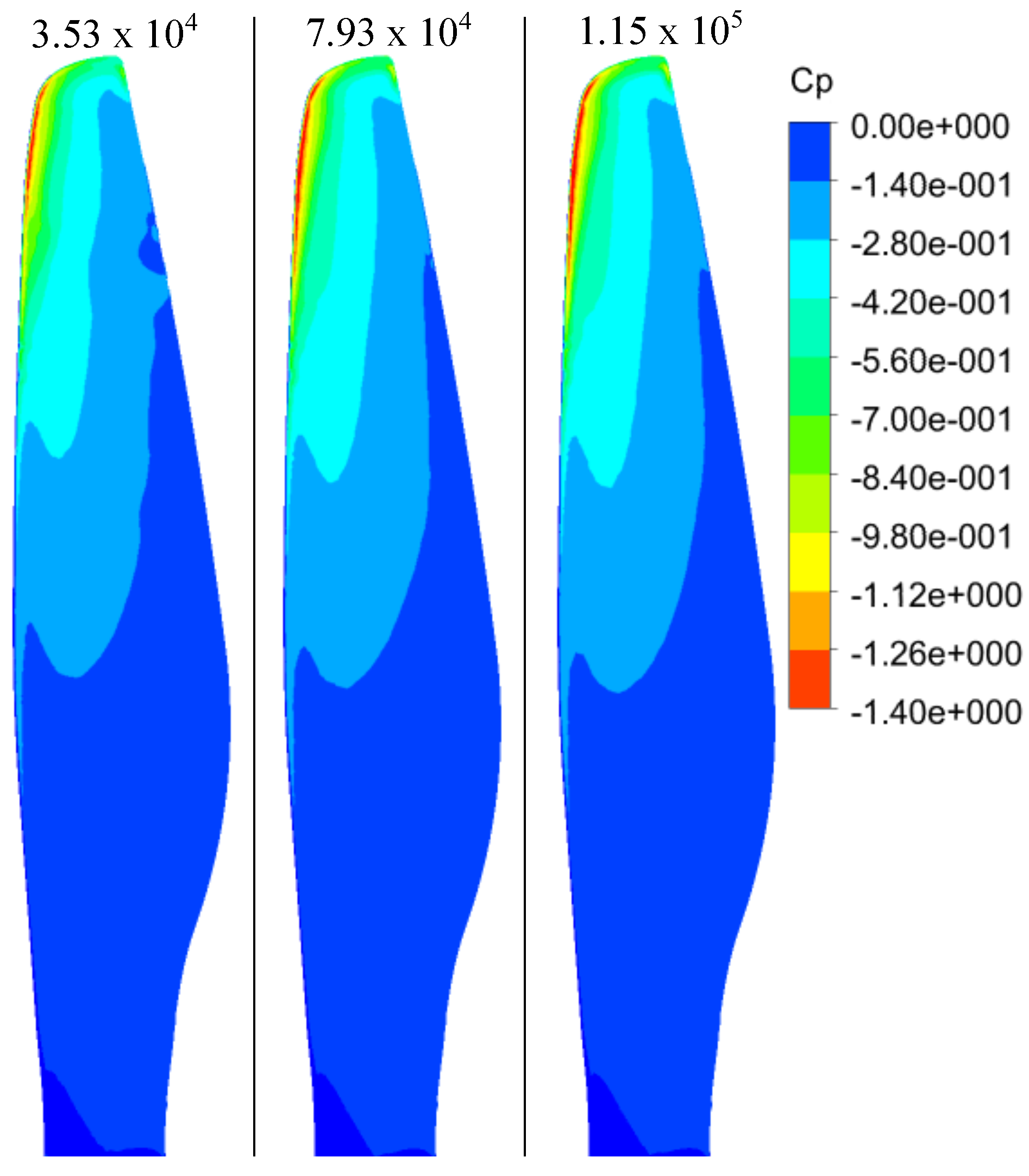
where P is the pressure; $P_{ref}$ is the reference pressure, in this case the ambient pressure; $\rho$ is the density; and $V_{ref}$ is a reference velocity, in this case the tip velocity, $wR$. Figure 7 and Figure 8 show contours of the pressure coefficient on the upper surface of the rotor for both turbulence models. It is clear that as the $Re$ increases, higher pressures cover slightly wider areas at the leading edge. Nevertheless, it is observed that as the $Re$ increases, the pressure distribution remains relatively stable—for example, compare the two highest values of $Re$. This tendency agrees with the asymptotic behavior shown in Figure 5 and Figure 6 for the thrust and torque coefficients as the $Re$ increases. It is also clear that the fully turbulent model over-predicts the pressure at the leading edge in comparison to the transitional model, especially at low angular velocities (low $Re$).

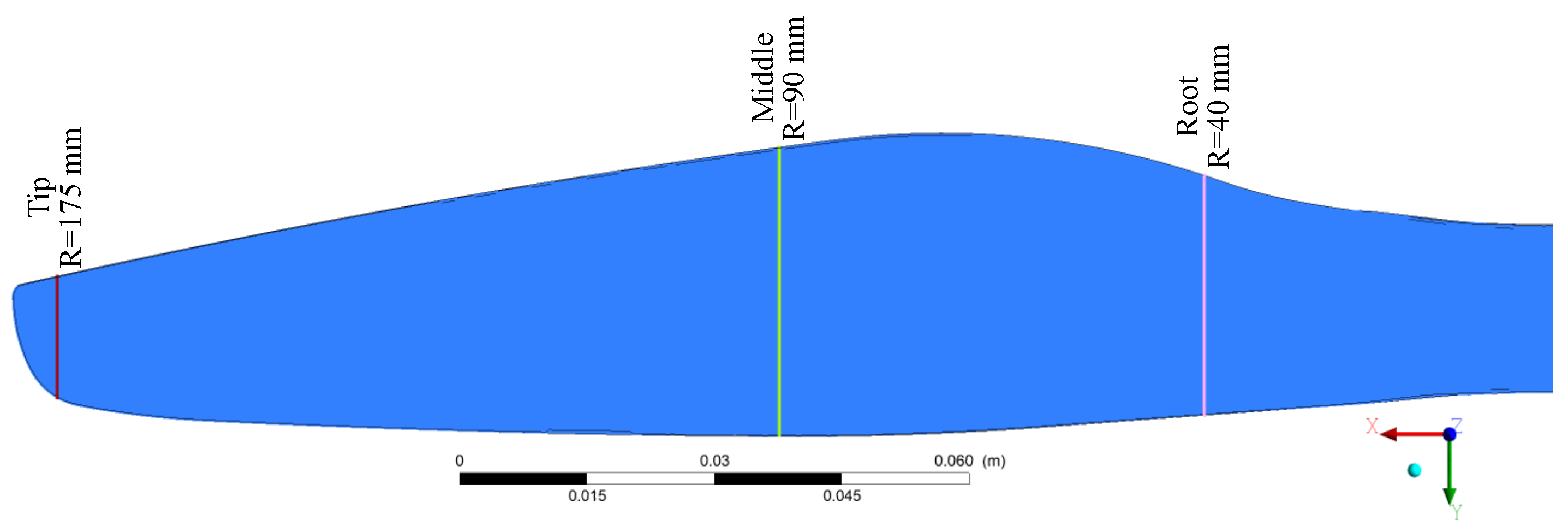
Three different sections along the span were selected to better compare the results from the transition and the fully turbulent models. These sections are located at the tip, mid-span, and root, as shown in Figure 9. Figure 10 shows how the pressure coefficient varies along the chord at the three sections for both turbulence models. The distance from the trailing edge to the leading edge was normalized using the chord length at that span location; therefore, at the trailing edge, $x/c=0$, and at the leading edge, $x/c=1$. Significant differences in $C_p$ predictions on the upper surface of the blade (in the tip section) can be observed between the turbulence models; however, these differences are reduced as the $Re$ increases. The peak suction pressure in the upper surface is always higher for the fully turbulent model. These differences could be an important issue when improving the rotor design for better performance at a low $Re$. At the tip’s leading edge, the generation of the tip vortices enhances the transition to turbulent flow; this could explain why at this zone and at a higher operational $Re$, the differences between the turbulent models are reduced.

On the lower surface, there are no significant differences in $C_p$ between the models, since the adverse pressure gradients are not as strong as on the upper surface. It is also observed that the highest pressure develops at the leading edge and decreases along the chord until it reaches suction values on a small zone at the trailing edge. Due to the high pressure difference between the upper and lower surface at the leading edge, a pitching moment is developed on the blade. This moment could affect the performance of the blade by modifying the effective angle of attack of the section of the blade.

3.2.3. Flow Separation Analysis

The skin-friction coefficient on the surface of the blade allows one to locate regions where boundary-layer separation possibly occurs. This coefficient is calculated as shown in Equation (10):

$$C_f=\frac{{\tau }_{wall}}{\rho V_{ref}^2},$$

(10)

where $V_{ref}$ is the reference velocity, which in this case is also the velocity at the tip, i.e., $wR$. Strong changes from positive to negative values of $C_f$ indicate possible zones where boundary-layer separation occurs. Alongside the skin-friction coefficient, surface streamlines can be used to confirm the locations where the boundary layer separates and reattaches to the blade surface; these methods are similar to experimental techniques based on oil flow.

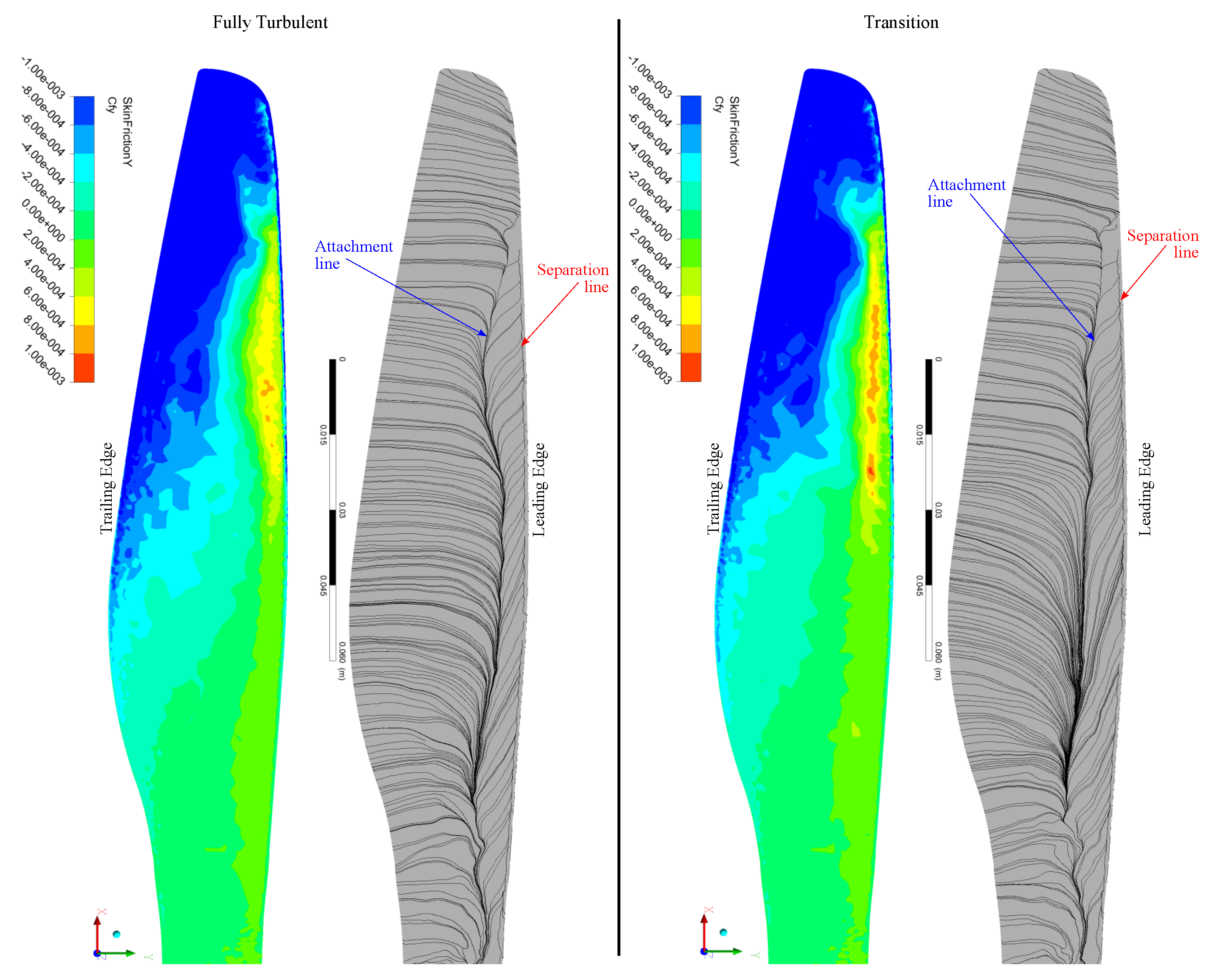
Figure 11 shows the skin-friction coefficient contours in the “Y” direction, and the surface streamlines on the upper surface for the fully turbulent model and the transition-turbulence model. Positive values of $C_f$ indicate that the boundary layer is attached to the wall. The transition-turbulence model predicts a clear separation zone at the tip’s leading edge. This zone is colored in blue on the skin-friction contours of Figure 11.

From surface streamlines, a separation line is observed on the leading edge and the line where the boundary layer re-attaches. This separation zone is also present for lower rotational velocities, though the attachment line is farther from the separation line; i.e., the boundary layer takes longer to re-attach. These features at the leading edge (close to the tip) are similar to those predicted by the fully turbulent model. The fully turbulent model does not show another separation region except close to root at the trailing edge. In contrast, the transition-turbulence model shows a clear separation line close to the trailing edge from the mid-span to the root. This is also evident in the skin-friction contours, showing a change in the sign of the skin-friction coefficient (cyan region) but not as strong as for the leading edge separation. Furthermore, these surface streamlines suggest a cross-flow zone with a high velocity in the "X" direction from the root to the mid-span. This cross-flow section is stronger close to the trailing edge, and it is also present for lower $Re$ approaching the tip as the $Re$ decreases. The fully turbulent model also presents this cross-flow but at lower $Re$ (not shown, further details are found on reference [19]), and as for the case of the transition-turbulence model, the cross-flow gets closer to the tip when the velocity reduces. Serre et al. [10] used oil flow visualization of a rotor that was tested at 5000 RPM; the rotor’s radius was $0.0875$ m. At the leading edge, an early separation zone was identified that had quick re-attachment, a turbulent boundary layer was developed, and a second separation zone was identified at the trailing edge. Those experimental results are closer to the computational results shown for the transition-turbulence model in the present study.

On the lower surface, the boundary layer was attached when $C_f$ was negative (see Figure 12). The transition-turbulence model shows that the boundary layer does not separate at the tip but at the mid-span and very close to the leading edge. A reattachment of the boundary layer happens close to the mid-chord. This behavior was also observed for lower $Re$ (not shown, but more details are found in reference [19]), but as the $Re$ increased, the attachment line moved closer to the leading edge. The strong cross-flow developed on the upper surface was not present on the lower surface, which could be related to the high level of twist of the blade close to the root. There are no important observable differences between the results of the turbulence models.

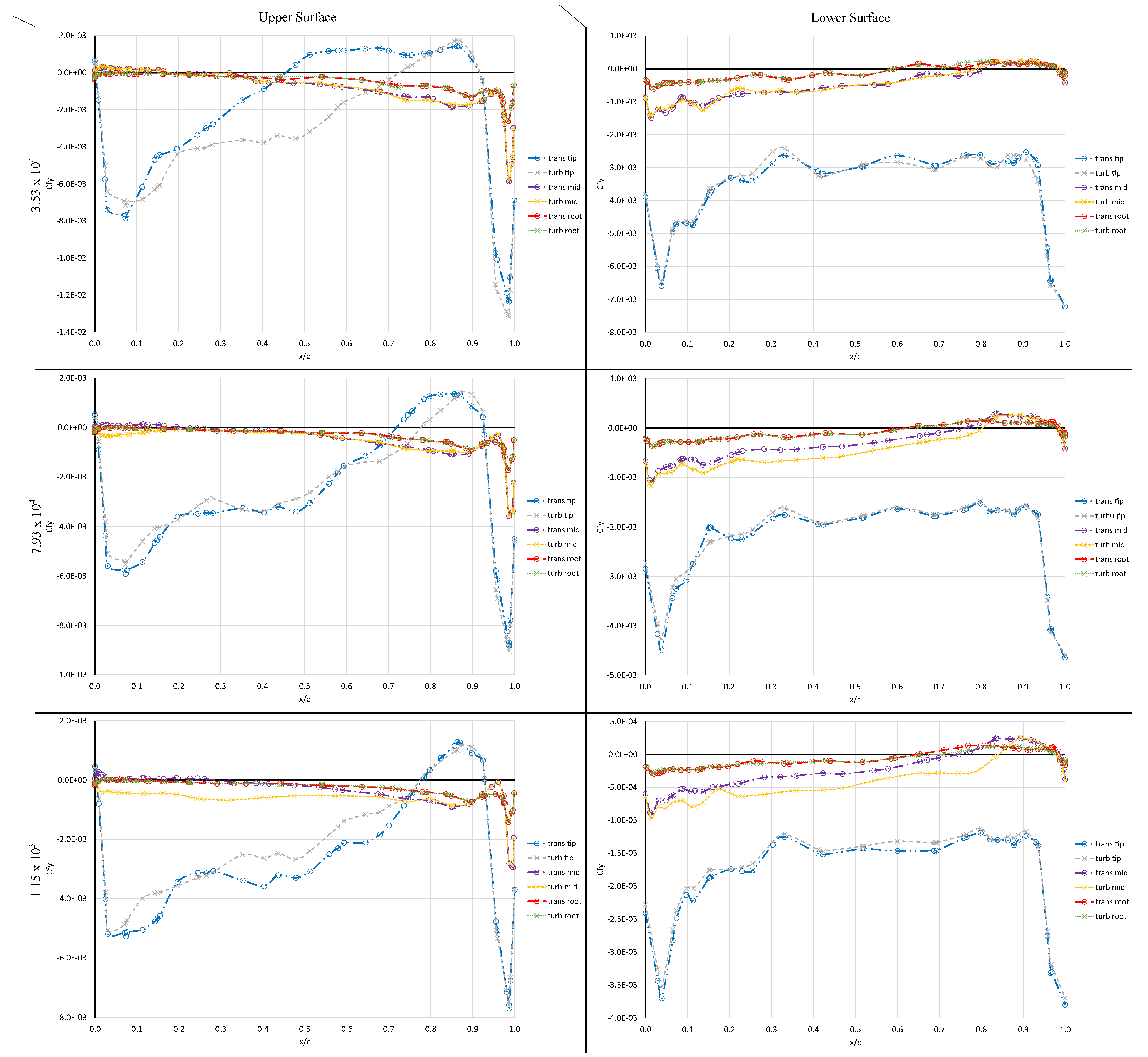
A more precise location of the boundary layer’s separation and re-attachment can be observed in Figure 13, in which the skin-friction coefficients at the same span-wise locations shown in Figure 9 for different rotational velocities and for both turbulence models are shown. It is clear that the main differences in the models’ predictions are for the upper surface close to the tip, though those differences are reduced as the $Re$ increases. However, on the upper surface, when $Re$ increases, both models predict different skin-friction behavior at the mid-span section; e.g., for $Re=1.15\times {10}^5$, whereas the transition-turbulence model predicts separation along close to $30\%$ of the chord, the fully turbulent model does not predict separation at all. For the lower surface, the results from both turbulence models are very similar. Nevertheless, at the mid-span section, some differences can be observed as the $Re$ increases. The main difference is the re-attachment location; for example, at $Re=1.15\times {10}^5$, the fully turbulent model predicts reattachment for close to $84\%$ of the chord, whereas the transition-turbulence model shows that the reattachment occurs for $75\%$ of the chord.

Boundary-layer separation causes losses in lift and increases the drag; therefore, the overall performance of the rotor is reduced. The separation bubble found at the tip’s leading edge is small, and then it re-attaches, but the boundary layer becomes turbulent. This separation could be promoted by the strong tip vortices developed by these rotors. From the mid-span to the root, the boundary layer separates close to the trailing edge, but it does not re-attach. Argus et al. [8] suggested that reduction of the separation zones and an early transition to a turbulent boundary layer lead to gains in rotor performance. However, the experimental study of Jaroslawski et al. [20] demonstrated that forcing the transition from laminar to turbulent with roughness leads to a significant reduction in the hover rotor efficiency. Therefore, the redesign of the tip and mid-span zones could lead to improvements in the rotor’s performance. Through computational simulations, it is possible to estimate the sizes of the separation bubbles; however, for rotors operating at low to medium Reynolds numbers, a transition-turbulence model could lead to better results, thereby improving rotor design.

3.3. Another Transition Model’s Results

Given the good performance and predictive capabilities of the SST $k-\omega$ transitional model, this section is focused on specific results obtained by that turbulence model. Two main elements are analyzed: boundary-layer prediction and wake dynamics.

Boundary-Layer Prediction

Intermittency is a parameter used to determine those regions where laminar and turbulent flows coexist and is one of the main variables of the SST $k-\omega$ transition model. For a laminar flow, the intermittency value is zero, and it is one for a fully turbulent flow. In this section, only results for the highest $Re$ number ($1.15\times {10}^5$) are discussed (this information for other $Re$ can be found in [19]).

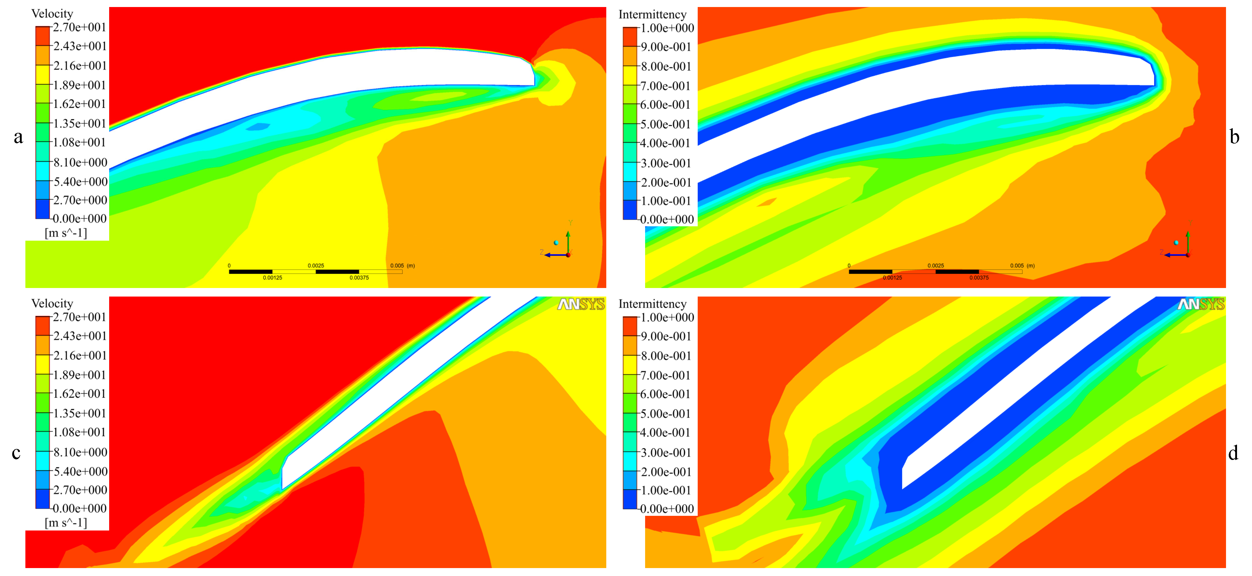
Figure 14, Figure 15 and Figure 16 correspond to transversal sections along the span of the blade; the locations of these sections are the same as those used in previous sections and shown in Figure 9. At the root where the rotor tangential velocity is lower, the upper surface boundary layer is laminar and thin at the leading edge, but it thickens and develops towards the trailing edge. On the lower surface, a laminar boundary layer is thicker than on the upper surface.

Mid-span on the upper surface, a laminar boundary layer is developed, and its thickness increases from the leading edge to the trailing edge. A small zone is developed, where velocity is low, showing a separation zone (highlighted as a circle in Figure 15); this feature was not developed for lower $Re$ (not shown; see reference [19] for more details). On the lower surface, the boundary layer remains laminar all along the chord.

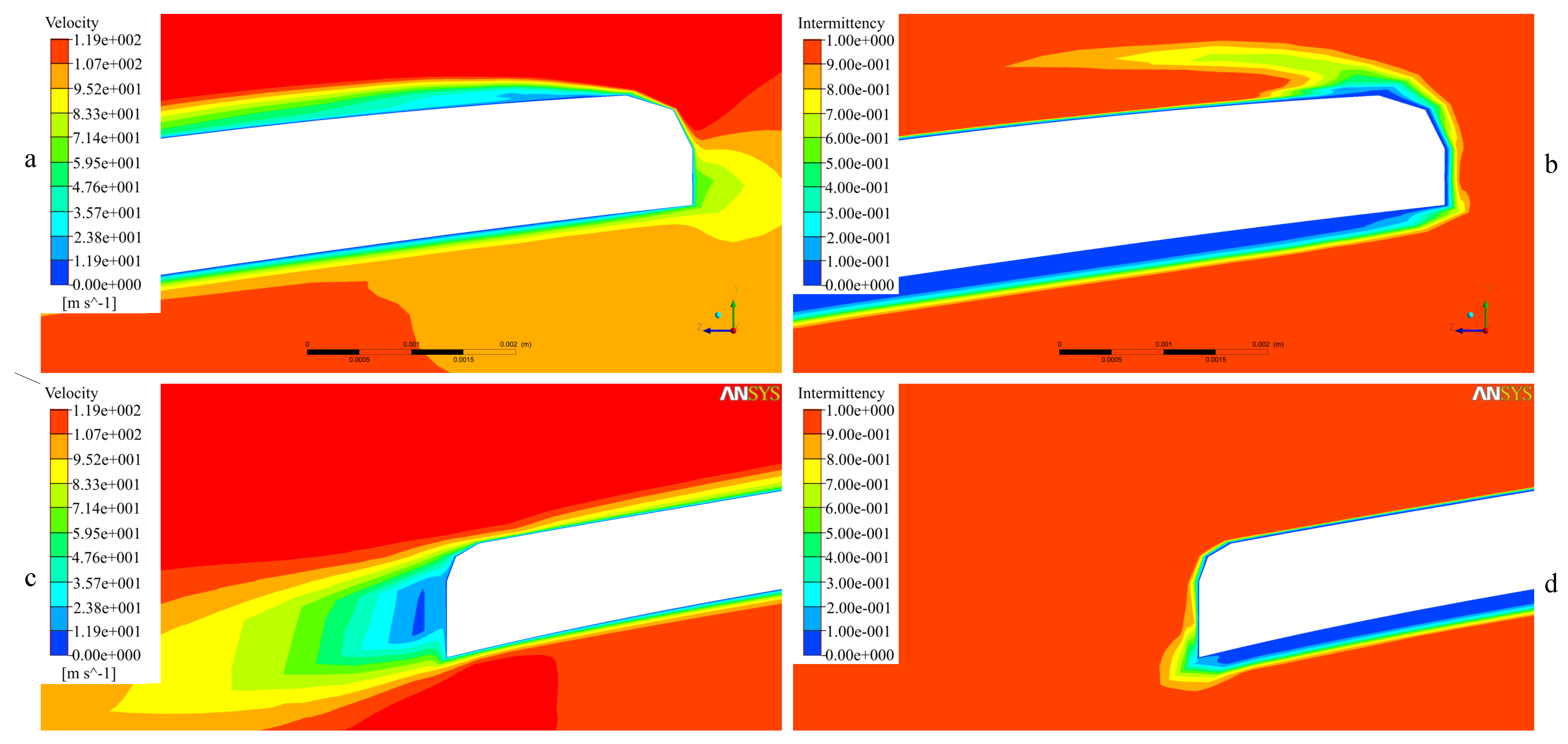
Figure 16 shows that on the upper surface and close to the tip and the leading edge, there is a zone with a strong change in intermittency contours, which could indicate a separation zone. After this zone, the boundary layer is turbulent and remains in this condition along the chord. On the lower surface, the velocity contours do not show sudden velocity changes; i.e., there is no flow separation, and the boundary layer is laminar along the chord.

From intermittency and velocity contours, it is concluded that the boundary layer is laminar for most of the blade’s span. At the leading edge, there is a thin boundary layer along the span, and it remains thin up to mid-way along the chord. From mid-span to the root close to the trailing edge, there is a thick boundary layer which could increase the profile drag [1]. However, a turbulent boundary layer is developed at the blade’s tip on the upper surface. This turbulent boundary layer is achieved after a small separation zone, which is also shown in Figure 11. At the tip where the velocities are higher and the tip vortices are generated, there is a rapid transition to a turbulent boundary layer. At trailing edge from root to mid-span, there is high level of twisting of the blade that increases the thickness of the boundary layer and could prevent the separation and transition of the boundary layer.

3.4. Wake Dynamics

Figure 17 shows the wake structure using an isocontour of the Q-criterion colored by vorticity magnitude for various $Re$. The main vortical structures that are observed correspond to the tip vortices with stronger structures for higher $Re$. The tip vortices’ intensity was higher close to the rotor tip, and decreased as it was convected in the wake. Another vortical structure that is clearly observed corresponds to a strong vortex generated at the blade root. The motor, which is attached to the rotor’s center, and the mechanical structure, to support the motor–rotor system, probably inhibit the formation of this vortex in the real operation of the rotor.

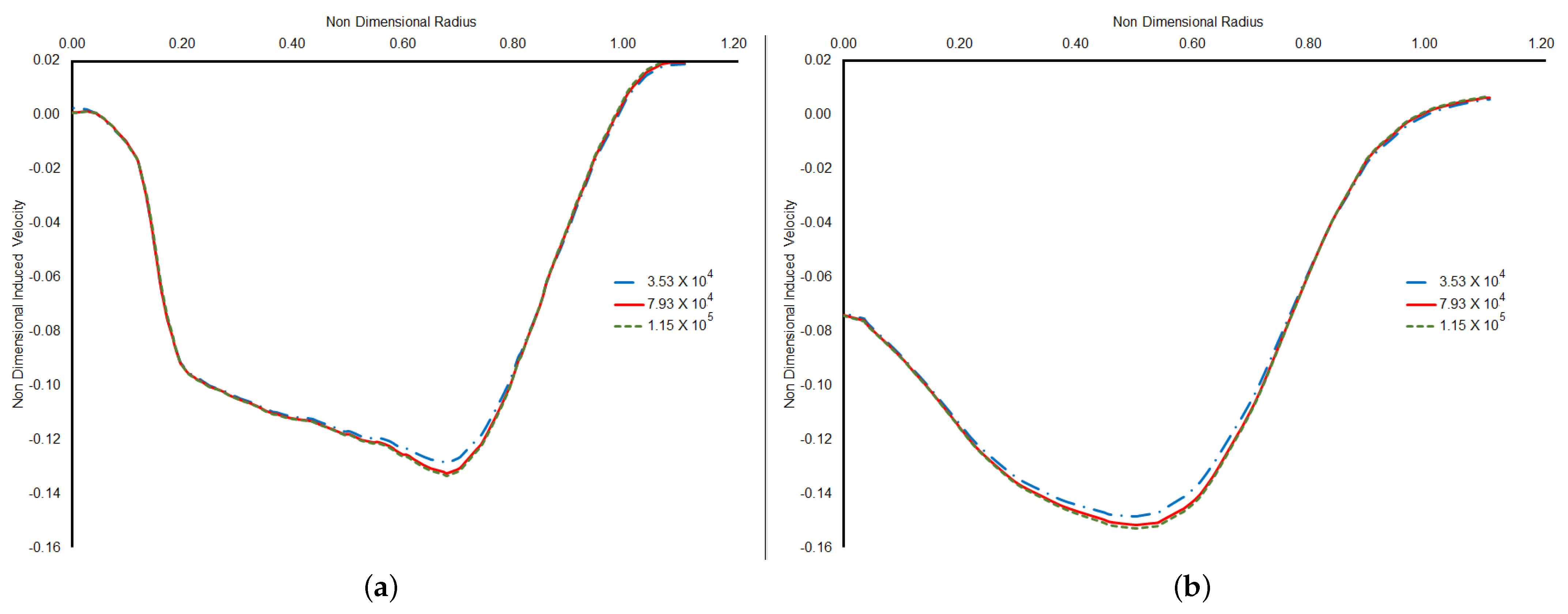
In order to visualize the development of the wake, the profile of the vertical component of the velocity at different vertical distances downstream the rotor disk was investigated. Figure 18 shows the induced velocity profiles as a function of radial position. Axial and radial positions were non-dimensionalized by the rotor radius R, and velocities by the blade tip velocity $wR$. Below the rotor disk at $0.1R$, the velocity was 0 at the center of the disk, and then there was a strong increase of up to $9.5\%$ in the tip velocity, reached at a $0.2R$. From $0.2R$ to $0.7R$, the velocity kept growing but at a lower rate. The highest velocity, which was $13\%$ of the tip velocity, was reached close to $0.7R$; after this location, the velocity decreased, reaching a value close to 0 at the tip. After the tip, the velocity direction changed due to tip vortices, reaching a maximum of $2\%$ upwash of tip velocity at a position of $1.1R$. For further distances downstream the rotor disk, the maximum velocity increased because of the wake contraction and momentum conservation, and it developed closer to the position $0.4R$. It is observed that the induced velocity variation is lower when $Re$ increases from $7.93\times {10}^4$ to $1.15\times {10}^5$ than when the increment is from $3.53\times {10}^4$ to $7.93\times {10}^4$. This small difference observed at higher rotational velocities could explain the asymptotic tendency developed for thrust and torque when the rotor operates at higher $Re$.

4. Conclusions

Successful computational simulations of a small rotor operating at hover and at different operational Reynolds numbers were performed using two different turbulent approximations, the transition and the fully turbulent versions of the SST $k-\omega$ turbulence model.

Numerical results were validated using the fully turbulent model only, showing that the predictions for thrust and torque are close to experimental measurements, within the uncertainty values. A closer evaluation of these computational results showed a clear influence of $Re$ and an asymptotic tendency to maximum torque and thrust as the $Re$ increases.

When comparing both turbulence models, it was observed that in general, the models have similar results with differences of less than 5% in the prediction of global performance variables such as thrust and toque. Nevertheless, the transition-turbulence model shows better agreement with the experimental measurements in the prediction of the same variables. Significant differences were observed between both models when studying the boundary-layer separation. At the tip, these differences are reduced as the $Re$ increases, but at mid-span, the differences increase as the $Re$ increases. Boundary-layer separation affects the performance of the rotor; therefore, it has been shown that a transition-turbulence model leads to better results than a fully turbulent model.

From intermittency and velocity contours on the blades obtained from the results of the transition-turbulence model, it was found that the boundary layer is laminar for most of the blade’s span. At the tip’s leading edge, a turbulent boundary layer is developed after a small separation zone, and at the trailing edge, a separation zone was identified from the mid-span to the root. This boundary layer behavior could affect the aerodynamic performance of the rotor, leading to reductions in the lift-to-drag ratio and an increase in the profile losses.

References

1. Ramasamy, M.; Johnson, B.; Leishman, J. Understanding the Aerodynamic Efficiency of a Hovering Micro-Rotor. J. Am. Helicopter Soc. 2008, 53, 412–428. [Google Scholar] [CrossRef]
2. Duraisamy, K.; Baeder, J. High Resolution Wake Capturing Methodology for Hovering Rotors. J. Am. Helicopter Soc. 2007, 52, 110–122. [Google Scholar] [CrossRef]
3. Potsdam, M.; Pulliam, T. Turbulence modeling treatment for rotocraft wakes. In Proceedings of the AHS Specialists Conference on Aerodynamics 2008, San Francisco, CA, USA, 23–25 January 2008; Volume 2. [Google Scholar]
4. Gomez, S.; Gilkey, L.; Kaiser, B.; Poroseva, S. Computational Analysis of a Tip Vortex Structure Shed from a Bio-inspired Blade. In Proceedings of the 32nd AIAA Applied Aerodynamics Conference, Atlanta, GA, USA, 16–20 June 2014. [Google Scholar] [CrossRef] [Green Version]
5. Liu, J.; Luo, S. Navier–Stokes Equations based Flow Simulations of Low Reynolds Number Propeller for Unmanned Aerial Vehicle. In Proceedings of the 55th AIAA Aerospace Sciences Meeting, Grapevine, TX, USA, 9–13 January 2017. [Google Scholar] [CrossRef]
6. Ahmed, K.H.; Rajendran, P. 3D CFD Simulation and Experimental Validation of Small APC Slow Flyer Propeller Blade. Aerospace 2017, 4, 10. [Google Scholar] [CrossRef] [Green Version]
7. Rovere, F.; Steijl, R.; Barakos, G.N. CFD Analysis of a micro rotor in ground effect. In Proceedings of the AIAA Scitech 2020 Forum, Orlando, FL, USA, 6–10 January 2020. [Google Scholar] [CrossRef] [Green Version]
8. Argus, F.J.; Ament, G.A.; Koning, W.J.F. The Influence of Laminar-Turbulent Transition on Rotor Performance at Low Reynolds Numbers. In Proceedings of the VFS Aeromechanics for Advanced Vertical Flight Technical Meeting, San Jose, CA, USA, 21–23 January 2020. [Google Scholar]
9. Henricks, Q.; Wang, Z.; Zhuang, M. Small-Scale Rotor Design Variables and Their Effects on Aerodynamic and Aeroacoustic Performance of a Hovering Rotor. J. Fluids Eng. 2020, 142. [Google Scholar] [CrossRef]
10. Serre, R.; Gourdain, N.; Jardin, T.; Jacob, M.; Moschetta, J.M. Towards silent Micro-Air Vehicles: Optimization of a low Reynolds number rotor in hover. Int. J. Aeroacoustics 2019, 18, 690–710. [Google Scholar] [CrossRef]
11. Garofano-Soldado, A.; Sanchez-Cuevas, P.J.; Heredia, G.; Ollero, A. Numerical-experimental evaluation and modelling of aerodynamic ground effect for small-scale tilted propellers at low Reynolds numbers. Aerosp. Sci. Technol. 2022, 126, 107625. [Google Scholar] [CrossRef]
12. Picard, A.; Davis, R.; Gläser, M.; Fujii, K. Revised formula for the density of moist air (CIPM-2007). Metrologia 2008, 45, 149. [Google Scholar] [CrossRef]
13. Luo, J.Y.; Issa, R.I.; Gosman, A.D. Prediction of Impeller-Induced Flows in Mixing Vessels Using Multiple Frames of Reference. IChemE Symp. Ser. 1994, 136, 549–556. [Google Scholar]
14. Menter, F.R. Two-equation eddy-viscosity turbulence models for engineering applications. AIAA J. 1994, 32, 1598–1605. [Google Scholar] [CrossRef] [Green Version]
15. Smirnov, P.E.; Menter, F.R. Sensitization of the SST Turbulence Model to Rotation and Curvature by Applying the Spalart-Shur Correction Term. ASME J. Turbomach. 2009, 131, 8. [Google Scholar] [CrossRef]
16. Menter, F.; Langtry, R.; Likki, S.; Suzen, Y.; Huang, P.; Völker, S. A Correlation-Based Transition Model Using Local Variables—Part I: Model Formulation. ASME J. Turbomach 2006, 128, 413–422. [Google Scholar] [CrossRef]
17. Pérez Gordillo, A.M.; Villegas Santos, J.S.; Lopez Mejia, O.D.; Suárez Collazos, L.J.; Escobar, J.A. Numerical and Experimental Estimation of the Efficiency of a Quadcopter Rotor Operating at Hover. Energies 2019, 12, 261. [Google Scholar] [CrossRef] [Green Version]
18. Perez, A.M.; Lopez, O.D.; Escobar, J.A. Computational Study of the Wake of a Quadcopter Propeller in Hover. In Proceedings of the 23rd AIAA Computational Fluid Dynamics Conference, Denver, CO, USA, 5–9 June 2017. [Google Scholar] [CrossRef]
19. Perez, A.M. Performance Characterization of the Propulsion System of a Quadcopter in Hover. Ph.D. Thesis, Universidad de los Andes, Bogota, Colombia, 2020. [Google Scholar]
20. Jaroslawski, T.; Forte, M.; Delattre, G.; Gowree, E.R.; Moschetta, J.M. Laminar to turbulent transition over a rotor at low Reynolds numbers. In Proceedings of the Aero 2020+1—55th 3AF International Conference on Applied Aerodynamics, Poitiers, France, 23–25 March 2020. [Google Scholar]
Figure 1. Experimental setup scheme.
Aerospace 10 00130 g001
Figure 2. Stationary and rotating reference frames.
Aerospace 10 00130 g002
Figure 3. Rotor.
Aerospace 10 00130 g003
Figure 4. Stationary and rotating reference frames.
Aerospace 10 00130 g004
Figure 5. Computational results for thrust coefficient as a function of Re.
Aerospace 10 00130 g005
Figure 6. Computational results for torque coefficient as a function of Re.
Aerospace 10 00130 g006
Figure 7. Pressure coefficient distribution on the upper surface of the rotor using the transition-turbulence model.
Aerospace 10 00130 g007
Figure 8. Pressure coefficient distribution on the upper surface of the rotor using the fully turbulent model.
Aerospace 10 00130 g008
Figure 9. Planes for different sections along the span.
Aerospace 10 00130 g009
Figure 10. Pressure coefficient along the chord for different sections along the span.
Aerospace 10 00130 g010
Figure 11. Skin-friction coefficient and surface streamlines for R e = 1.15 × 10 5 on the upper surface.
Aerospace 10 00130 g011
Figure 12. Skin-friction coefficient and surface streamlines for R e = 1.15 × 10 5 on the lower surface.
Aerospace 10 00130 g012
Figure 13. Skin-friction coefficient along the chord for different sections along the span.
Aerospace 10 00130 g013
Figure 14. Velocity and intermittency contours at the root for operation at R e = 1.15 × 10 5 . (a) Velocity at the leading edge, (b) intermittency at the leading edge, (c) velocity at the trailing edge, (d) intermittency at the trailing edge.
Aerospace 10 00130 g014
Figure 15. Velocity and intermittency contours at mid-span for operation at R e = 1.15 × 10 5 . (a) Velocity at the leading edge, (b) intermittency at the leading edge, (c) velocity at the trailing edge, (d) intermittency at the trailing edge.
Aerospace 10 00130 g015
Figure 16. Velocity and intermittency contours at the tip for operation R e = 1.15 × 10 5 . (a) Velocity at the leading edge, (b) intermittency at the leading edge, (c) velocity at the trailing edge, (d) intermittency at the trailing edge.
Aerospace 10 00130 g016
Figure 17. Q-criterion contours, colored by vorticity magnitude: (a) R e = 3.53 × 10 4 , (b) R e = 7.93 × 10 4 , (c) R e = 1.15 × 10 5 .
Aerospace 10 00130 g017
Figure 18. Comparison between induced velocity for different rotational velocities. (a) At 0.1R below the rotor, (b) 0.5R below the rotor.
Aerospace 10 00130 g018