Investigations of the Atomization Characteristics and Mechanisms of Liquid Jets in Supersonic Crossflow

Abstract

In the combustion chamber of scramjets, fuel jets interact with supersonic airflow in the form of a liquid jet in crossflow (LJIC). It is difficult to achieve adequate jet–crossflow mixing and the efficient combustion of fuel in an instant. Large eddy simulation (LES), the coupled level-set and volume of fluid (CLSVOF) method, and an adaptive mesh refinement (AMR) framework are used to simulate supersonic LJICs in this article. This way, LJIC atomization characteristics and mechanisms can be further explored and analyzed in detail. It is found that the surface waves of the liquid column exist in a two-dimensional form, including vertical and spanwise directions. Column breakup occurs when all the spanwise surface waves between adjacent vertical surface waves break up. Bow shock waves, composed of multiple connected arcuate shock waves, are dynamic and will change with the evolution of the liquid column. The vortex ring movement of supersonic LJICs, whose trends in the vertical and spanwise directions are different, is relatively complex, which is due to the complex and time-dependent shape of liquid columns.

1. Introduction

Scramjets, which can obtain oxygen from the atmosphere during the climbing process, are characterized by being structurally simple, lightweight, cost-effective, and high-speed. A scramjet can generate four times the thrust of a rocket when consuming the same mass of propellant. In the combustion chamber of a scramjet, the residence time of the fuel is only in milliseconds due to a supersonic crossflow. Therefore, how to promote and enhance the fuel–air mixing in the shortest possible time is a major challenge in supersonic combustion. Adequate fuel atomization and a uniform droplet size are the prerequisites of efficient combustion, which are conducive to fuel–air mixing. However, up to now, the fuel atomization in supersonic crossflows can be influenced by many factors, and it is not easy to observe and measure the spray field, which is a transient, dense spray area. The mechanism research on the liquid hydrocarbon fuel atomization process in supersonic crossflows is still limited, which is far from meeting the needs of supersonic combustion theoretical research and actual engine design.

In the scramjet combustion chamber, the fuel jet interacts with a supersonic airflow in the form of an LJIC. Under strong shear and acceleration of the crossflow, the fuel jet bends, deforms, breaks, atomizes, and finally forms droplets with micron size. In the process of breakup and atomization, the liquid jet undergoes multi-scale deformation from millimeter to micrometer. Under the coupling effect of aerodynamic acceleration and gas–liquid shear, liquid column breakup and surface breakup occur simultaneously. Due to the obstruction of the liquid column, complex flow field structures, such as bow shock and separated shock, are generated, as shown in Figure 1.

Liquid jets in crossflow (LJICs) are a major subject of fluid mechanics. Fuel atomization in the form of LJICs, as the primary stage of the energy conversion of fuel, is of great significance for combustion efficiency and stability. Studying the atomization characteristics and mechanisms of supersonic LJICs has a promoting effect on engine design. Extensive research has been conducted by scholars on this issue.

Experimental methods have been adopted by some researchers to investigate supersonic LJICs. The phase Doppler anemometry (PDA) method was employed by Li [1] to conduct an experimental study on the atomization characteristics of supersonic LJICs; it was found that the spray cross-section, whose height and width increase linearly with the increase in the nozzle diameter, was approximately Ω-shaped. The particle image velocimetry (PIV) technology was applied by Wang [2] to observe the velocity and structure of water jets in a crossflow at Ma = 2.1; it was found that the spray velocity accelerated rapidly to 66% of the crossflow in the position of 15 times the nozzle diameter and increased slowly in the far field under the action of the jet’s driving force and gas–liquid shear. An oscillation distribution model was established by Wu [3,4] to quantitatively describe the jet oscillation distribution characteristics with the help of the pulsed laser background imaging method and the tilt imaging method. Wu [5] found that the distribution shape of the Sauter mean diameter (SMD) of a kerosene jet in a crossflow at Ma = 1.86 changed from being C-shaped to I-shaped with the evolution of atomization using the phase Doppler wind speed method. The oil–air interface data and bow wave data were obtained by Hui [6] to explore the fuel injection driving mechanism ulteriorly using the quantitative Schlieren method based on a direct connected wind tunnel.

An LJIC primary atomization simulation was carried out by Nambu [7] to reveal the characteristics of RT instability, which generates surface waves. A detailed numerical simulation (DNS) was used by Behzad [8] to investigate the surface breakup mechanism, and the results showed that the shear instability was dominant. The primary atomization was investigated by Mukundan [9] using direct DNS and LES, and the column breakup and surface breakup were revealed as the two main synchronous atomization mechanisms. The CLSVOF method and LES were used by Xiao [10] to explore LJIC primary breakup. It was found that the surface waves originated from RT instability. The atomization process was simulated by Wen [11] using the Euler–Lagrangian framework to probe the effect of the Weber number on atomization. LES, VOF, and AMR were used by Jadidi [12] to explore the influence of the gas/liquid density ratio on the jet trajectory, and the results showed that the penetration increased with an increasing density ratio.

The volume method, as an important means of numerical research on supersonic LJICs, is widely used by scholars. Zhao [13] found that a counter-rotating vortex pair (CVP), which accelerated the spray-mixing process, was generated inside the spray by using the CLSVOF method based on delayed separated eddy simulation (DDES). The shock waves in front of the droplets and ligaments were captured, and two types of vortices related to surface breakup and column breakup were observed by Xiao [14,15] using the CLSVOF method; it was found that the pressure distributions around the liquid column resulting from the crossflow compressibility were different at different Mach numbers, and as the crossflow Mach number increased, the liquid column penetration raised first and then lowered. By using the VOF method, Li [16] found that the primary breakup could be divided into surface breakup dominated by KH instability and column breakup dominated by RT instability, and the cause of the surface waves was a fluctuation in the local pressure on the jet surface. It was discovered by Zhou [17] that the length of the round, smooth liquid column at the entrance increased with the increase in the injection pressure, and the near-wall CVP could intensify the jet breakup. The discrete phase method, characterized by accurate tracking on droplets, is becoming increasingly popular. With the help of the Euler–Lagrange method, Li [18,19,20] discovered that the crossflow streamlines intersected with the droplet trajectory and deflected towards the near-wall region, resulting in a wire-drawing phenomenon, and some droplets were transported to the near-wall area and then to both sides of the spray core area by two CVPs. Liu [21] found that the penetration, spanwise angle, and expansion area of a cavity-based kerosene jet in a supersonic crossflow increased with increasing injection pressure by using an improved KH-RT model.

Recently, the impact of the injection approach of jets on atomization has attracted increasing attention, which could provide guidance for the enhancement of two-phase mixing. By combining CLSVOF with an improved KH-RT model, Zhu [22,23] found that the penetration, span angle, and expansion area increased with increases in the injection angle and nozzle diameter, while that of the droplet size was the opposite. Zhou [24] found that jets with a larger aspect ratio had a smaller penetration and breakup length but a larger horseshoe vortex and wake region when using the CLSVOF method. An Euler–Lagrange method based on the KH-RT breakup model was used by Niu [25] to explore LJIC atomization, and it was found that the penetration was sensitive to the nozzle diameter, injection velocity, and mass flow rate. Almanzalawy [26] found that liquid jets with a core air flow and annular air flow could improve the spray breakup rate and spray size by employing a DDES model. With the help of the CLSVOF method, it was found by Zhu [27] that the pulsed liquid jet could promote atomization and jet–crossflow mixing performance, which was reflected in a 20% penetration increment and a 25% wake zone increment. The fact that the additional instability waves, which could improve the liquid column breakup, were imposed by pulsed jets was found by Liu [28] using a five-equation model based on the AMR framework, which is based on the usual conservation laws for mixture (mass, momentum, and energy balance), supplemented with a one-phase mass conservation equation and a transport equation for the volume fraction [29]. It was found by Lin [30] that an enhanced surface breakup, liquid column breakup, and shorter breakup length could be obtained with a pulsed jet with the help of the LES and CLSVOF methods. Hu [31] found that a gas-accompanied jet could improve jet penetration significantly using high-speed photography technology. Zhao [32,33], by employing high-speed imaging and the Euler–Lagrange method, found that hydrogen–water jets could enhance the penetration and mixing effects, especially via constant-flow countercurrent injection.

Shadow photography technology and a laser Doppler velocimeter were used by Almeida [34] to reveal that the breakup of jets was influenced more by the injection angle than by the liquid/gas momentum flux ratio. Schlieren technology and PIV were employed by Beloki Perurena [35], and the impact of the nozzle shape on jet atomization was studied. Comprehensive experiments were conducted by Olyaei [36] to explore the primary breakup characteristics of LJICs generated with different nozzle shapes. An experiment of circular and elliptical jets was conducted by Jadidi [37], and it was concluded that the nozzle aspect ratio could change the penetration significantly. High-speed imaging and shadow photography were used by Prakash [38] to explore the influence of laminar flow and turbulent flow. A modulation device was used by Lee [39] to conduct a study on modulated jets, and it was found that the periodic pressure could promote liquid–gas mixing. Phase Doppler particle analysis (PDPA) and a high-speed CCD camera were employed by Lee [40] to study the influence of pulsed air on liquid jets.

Extensive investigations have been conducted which, to some extent, explore the mechanisms of LJIC breakup and atomization, but there are still shortcomings. Firstly, the revelation of the atomization characteristics and mechanisms is still insufficient, and further in-depth analysis is needed. Secondly, water is chosen in most research as the jet liquid, while kerosene is used in real combustion chambers, which will lead to noteworthy differences in some parameters, such as the Weber number, Reynolds number, momentum flux ratio, etc. In addition, vortex characteristics, which have a significant impact on gas–liquid mixing, should receive more attention, as they have a guiding significance for engineering applications such as fuel combustion and jet control in scramjets. Therefore, an in-depth analysis of supersonic LJICs using LES, CLSVOF, and AMR is conducted in this manuscript, aiming to reveal the supersonic LJIC atomization characteristics and mechanisms ulteriorly.

2. Model and Numerical Methods

2.1. Model

The nozzle diameter is much smaller in scale compared to the entire flow field, and the flow area affected by the jet is also smaller in supersonic LJICs. To ensure both calculation accuracy and cost efficiency, a rectangular area, as shown in Figure 2, is taken as the calculation domain. The injection position is located at the coordinate origin O. The range of X, Y, and Z in three directions is [−8d, 16d], [0, 24d], and [6d, 6d].

The boundary conditions for numerical simulation are shown in

Table 1. The boundary conditions.

Boundary	Type
Crossflow inlet	Pressure inlet
Liquid jet inlet	Velocity inlet
Wall	No slip condition
Symmetry	Symmetry
Outlet	Pressure outlet

. The X-, Y-, and Z-directions correspond to the crossflow, vertical, and spanwise directions, respectively.

The nozzle diameter is d, aspect ratio (L/d) is 4, and the jet liquid is kerosene. The surface tension of kerosene is 0.026 N/m, the density of kerosene is 780 g/m³, the viscosity of kerosene is 0.0024 Pa∙s, and the jet velocity is 56.3 m/s. Level 4 AMR is adopted to improve the accuracy of the gas–liquid interface. The initial mesh before adaptation is 3.8 million. The time step is 1 × 10⁻⁸ s initially and then adapts automatically.

Due to the advantages of a high energy density, room temperature storage, safety, and convenience, kerosene is regarded as an appropriate propellant for scramjets and has extensive prospects for this application. Water is chosen by most researchers, although it can lead to differences in many parameters. Therefore, kerosene is chosen as the jet liquid in this article.

2.2. Numerical Methods

Supersonic crossflow is regarded as a compressible phase, whose general Navier–Stokes equation is as follows:

$$\frac{\partial \rho }{\partial t}+\frac{\partial \rho u_i}{\partial x_i}=0$$

(1)

$$\frac{\partial \left(\rho u_i\right)}{\partial t}+\frac{\partial \rho u_i{u}_j}{\partial x_j}=-\frac{\partial p}{\partial x_i}+\frac{\partial \left({\tau }_{ij}\right)}{\partial x_j}$$

(2)

$$\frac{\partial \left(\rho E\right)}{\partial t}+\frac{\partial \left(\rho E{u}_i\right)}{\partial x_j}=-\frac{\partial p{u}_i}{\partial x_i}+\frac{\partial \left(u_j{\tau }_{ij}\right)}{\partial x_i}-\frac{\partial q_i}{\partial x_i}$$

(3)

The numerical methods adopted in this article to simulate supersonic LJICs, such as LES, CLSVOF, and AMR, are introduced as follows:

The N-S equation is filtered to obtain a solvable scale control equation via LES, in which small-scale fluctuations can be filtered out. The filtering process, which can be presented using integration operations, is as follows:

$$\overline{u_i}(x,t)=\frac{1}{{\mathsf{\Delta }}^3}{\int }_{-\frac{\mathsf{\Delta }}{2}}^{\frac{\mathsf{\Delta }}{2}}{\int }_{-\frac{\mathsf{\Delta }}{2}}^{\frac{\mathsf{\Delta }}{2}}{\int }_{-\frac{\mathsf{\Delta }}{2}}^{\frac{\mathsf{\Delta }}{2}}{u}_i\left(\mathsf{\xi },t\right)G\left(x-\mathsf{\xi }\right)d{\mathsf{\xi }}_{1}d{\mathsf{\xi }}_{2}d{\mathsf{\xi }}_3$$

(4)

where $G\left(x-\mathsf{\xi }\right)$ is the filter function. For the integration filtering process of a cube with side length Δ, the expression is as follows:

$$G(\eta )=\left\{\begin{array}{c}1,\left|\eta \right|\le \Delta /2\\ 0,\left|\eta \right|\ge \Delta /2\end{array}\right.$$

(5)

LES filters out small-scale fluctuations, resulting in the LES control equation, as follows:

$$\frac{\partial \overline{u_i}}{\partial t}+\frac{\partial \overline{u_i{u}_j}}{\partial x_j}=-\frac{1}{\rho }\frac{\partial \overline{p}}{\partial x_i}+v\frac{{\partial }^2\overline{u_i}}{\partial x_j\partial x_i}+\overline{f_i}$$

(6)

$$\frac{\partial \overline{u_i}}{\partial x_i}=0$$

(7)

The mass conservation equation, momentum conservation equation, and energy conservation equation after Favre filtering can be written as follows:

$$\frac{\partial \overline{\rho }}{\partial t}+\frac{\partial \overline{\rho }{\tilde{u}}_j}{\partial x_j}=0$$

(8)

$$\frac{\partial \overline{\rho }{\tilde{u}}_i}{\partial t}+\frac{\partial \overline{\rho }{\tilde{u}}_i{\tilde{u}}_j}{\partial x_j}=-\frac{\partial \overline{p}}{\partial x_i}+\frac{\partial }{\partial x_j}({\tilde{\tau }}_{ij}-{\tau }_{ij}^{sgs}+D_{ij}^{sgs})$$

(9)

$$\frac{\partial \tilde{E}}{\partial t}+\frac{\partial (\tilde{E}+\overline{p}){\tilde{u}}_j}{\partial x_j}=\frac{\partial }{\partial x_i}(-{\tilde{q}}_i+{\tilde{u}}_j{\tilde{\tau }}_{ij}+{\mathcal{I}}_i^{sgs}+{\sigma }_i^{sgs}-Q_i^{sgs}-H_i^{sgs})$$

(10)

If $\overline{f}$ is a spatial filtering variable and $\tilde{f}$ is the density-weighted Favre filtering variable, then $\tilde{f}=\overline{\rho f}/\overline{\rho }$. The superscript “sgs” represents the unclosed term in the subgrid. Where ρ, u_i, and p are density, velocity, and pressure, respectively, ${\tilde{\tau }}_{ij}$ is a viscous flux term, ${\tilde{q}}_i$ is the heat flux term, and E is the total energy.

The expression for the unclosed term in the subgrid appearing in the filtering equation is as follows:

The subgrid stress term is

$${{\tau }_{ij}}^{sgs}=\overline{\rho }(\widetilde{u_i{u}_j}-{\tilde{u}}_i{\tilde{u}}_j)$$

(11)

The subgrid energy flux term is

$$H_i^{sgs}=C_p(\widetilde{\overline{\rho }{u}_{i}T}-\overline{\rho }{\tilde{u}}_i\tilde{T})$$

(12)

The subgrid turbulent diffusion term is

$${\mathcal{I}}_i^{sgs}=-\frac{1}{2}\overline{\rho }(u_i\widetilde{u_k{u}_k}-{\tilde{u}}_i\widetilde{u_k{u}_k})$$

(13)

The subgrid viscous stress term is

$${D_{ij}}^{sgs}={\overline{\tau }}_{ij}-{\tilde{\tau }}_{ij}$$

(14)

The subgrid heat flux term is

$$Q_i^{sgs}={\overline{q}}_i-{\tilde{q}}_i$$

(15)

The subgrid viscous diffusion term is

$${\sigma }_i^{sgs}=\overline{u_j{\tau }_{ij}}-{\tilde{u}}_j{\tilde{\tau }}_{ij}$$

(16)

${{\tau }_{ij}}^{sgs}$, $H_i^{sgs}$, and ${\mathcal{I}}_i^{sgs}$ are the unclosed terms that need to be modeled. ${D_{ij}}^{sgs}$, $Q_i^{sgs}$, and ${\sigma }_i^{sgs}$ are the unclosed terms that would be ignored due to their relatively small contribution. After the modeling and ignoring process, the compressible N-S equation after Favre filtering is closed.

In the current two-phase flow simulation method, the CLSVOF method, in which LS function Φ and VOF function F are introduced, is used to track the liquid–gas interface [41]. The LS function, Φ, is a variable sign distance function to the gas–liquid interface, while the VOF function, F, is the percentage of liquid volume in each cell.

Cartesian coordinates are used in two-phase solvers. The variables in the liquid-phase solver are located in a staggered manner, including the velocity components (u, v) on the cell surface and other variables (p, F) at the cell center. The variables (p, U, V) in the gas-phase solver are all located at the corners of the cell.

The VOF transport equation is as follows:

$$\frac{\partial F}{\partial t}+U_i\frac{\partial F}{\partial x_i}=0$$

(17)

The LS transport equation is as follows:

$$\frac{\partial \Phi }{\partial t}+U_i\frac{\partial \Phi }{\partial x_t}=0$$

(18)

To ensure the distance function characteristics of the LS function, it is necessary to solve the LS reinitialization equation, as follows:

$$\frac{\partial q}{\partial t}=S({\phi }_0)(1-\left|\nabla \phi \right|)$$

(19)

$$S({\phi }_0)=\frac{{\phi }_0}{\sqrt{{{\phi }_0}^2+d^2}}$$

(20)

where ${\phi }_0=\phi (\overrightarrow{x},\tau =0)=\Phi (\overrightarrow{x},t)$, $d=max(∆x,∆y)$, and τ is pseudo time. When the above reinitialization equation is solved to a stable state, set Φ to be equal to φ, i.e., $\Phi \left(\overrightarrow{x},t\right)=\phi (\overrightarrow{x},\tau =\infty )$.

The coupling process between LS and VOF is shown in Figure 3, and the concrete steps are as follows [42]: (1) Initialize LS function Φⁿ⁼⁰ and VOF function Fⁿ⁼⁰ at time step n = 0. (2) In the cutting calculation cell (0 < Fⁿ⁼⁰ < 1), a plane interface is constructed, whose normal vector and position are calculated via the LS function and VOF function, respectively. (3) The LS function (Φⁿ⁺¹)* and the VOF function (Fⁿ⁺¹) at the n+1 time step are obtained by solving the LS transport equation and the VOF transport equation. (4) In the cutting calculation cell (0 < Fⁿ⁺¹ < 1), plane interfaces are constructed by using (Φⁿ⁺¹)* and Fⁿ⁺¹. (5) Set the LS value in the cutting calculation cell (0 < Fⁿ⁺¹ < 1) as the geometric distance from the cell center to the constructed interface, and then solve the reinitialized equation to obtain the LS distribution with distance function properties, Φⁿ⁺¹.

The interface reconstruction is performed via the VOF method and the level-set method. The location of the phase interface is determined via the VOF method and the normal direction of the phase interface is determined via the level-set method. The process of reconstructing the phase interface is as follows: (1) The grid corresponding to the phase interface, whose volume fraction is between 0 and 1, is determined based on the VOF function value. (2) The normal values of the phase interface curves in the grid are confirmed by using the level-set function. (3) The curves that divide the grid are identified to ensure that at least one corner of the grid is occupied by the specified phase in adjacent grids. (4) The intersection point between the normal of the grid centerline pointing in the direction of the phase interface and the phase interface is located to meet the VOF function. (5) The intersection points between the phase interface and the grid boundary are used as boundary points for the reconstructed phase interface.

The LES result is largely influenced by the filtered mesh scale, which depends on a certain function of the mesh size [43,44,45,46]. In other words, the calculation result is directly influenced by the mesh size and distribution. Therefore, an unreasonable mesh will give rise to the loss of non-ignorable small-scale information, the loss of the fine features of LES, and a lack of rationality and reliability.

The process of jet atomization is accompanied by a large number of irregular and dynamically changing small-scale droplets, so it is impossible to predict the positions that need to be refined in advance. However, such challenges can be solved using AMR technology, through which dynamic mesh adjustments can be achieved based on pre-set evaluation criteria and calculation speeds that are several times faster than structural meshes can be achieved with the same accuracy [47]. This way, high precision and computational economy are ensured simultaneously. The AMR based on the octree method [48,49] used in this manuscript has the advantage of easily further discretizing existing meshes to improve efficiency and save costs. Octree meshes can coexist with Cartesian meshes, making it easy to track interfaces. Meshes after AMR can be considered a multi-layer structure and exist simultaneously in the computational domain, which is shown in Figure 4.

AMR can be divided into mesh coarsening and mesh refinement. The parent meshes can be refined to the sub meshes, and the sub meshes can be restored to the parent meshes. The level difference between adjacent meshes can only be less than or equal to 1. The mesh size needs to meet the following requirements:

$$\frac{\mathsf{\Delta }{x}_{l+1}}{\mathsf{\Delta }{x}_l}=\frac{\mathsf{\Delta }{y}_{l+1}}{\mathsf{\Delta }{y}_l}=r$$

(21)

2.3. Verification of Mesh Independence and Accuracy

The independence of the meshes is verified to ensure the calculation accuracy without being affected by the meshes. The initial mesh number of the computational domain is 3.8 million. Water is used as the liquid phase, the jet velocity is 56.3 m/s, and the crossflow Mach number is 2.85. Level 3, Level 4, and Level 5 AMR based on the volume fraction gradient are tested, respectively. The higher the AMR level, the higher the simulation accuracy, but the higher the mesh density and computational cost.

The Y-direction velocity calculation results at symmetry plane X/D = 0 of Level 3, Level 4, and Level 5 AMR are shown in Figure 5. From the figure, it can be seen that there are non-ignorable errors in the Level 3 AMR results, while the results of the Level 4 and Level 5 AMR are very close, indicating that Level 4 AMR meets the requirements and satisfies mesh independence. Level 4 AMR is adopted in this article to balance the accuracy and computational workload.

An LES algorithm, the CLSVOF method, and an AMR framework are used to simulate supersonic LJICs at Ma = 2.85 in this manuscript, and the penetration result is compared with the data of Li [16]. Good data consistency is achieved, as shown in Figure 6, indicating the sufficient accuracy of the model and a reliable numerical method for future research.

3. Results and Discussion

3.1. Breakup Process and Atomization Mechanism of Supersonic LJICs

It is urgent to have more insight into the LJIC mechanism of breakup and atomization, which can guide us towards adequate jet–crossflow mixing and the efficient combustion of fuel. An in-depth analysis of the numerical simulation results is conducted in this section, aiming to reveal the LJIC mechanism of breakup and atomization further.

3.1.1. Breakup Process of Supersonic LJIC

The near-field jet evolution process, which corresponds to 35.7 μs, 41.0 μs, 49.5 μs, 61.6 μs, 70.0 μs, and 80.2 μs, respectively, is shown in Figure 7, which is presented from a side view, front view, and top view. From Figure 7, it can be observed that, as time goes on, the vertical height of the liquid column increases and deflects downstream under the action of the crossflow, and the spanwise width of the jet increases with the increase in the vertical height and crossflow distance until the breakup of the liquid column occurs.

3.1.2. Atomization Mechanism of Supersonic LJIC

The jet’s three-dimensional shape and a jet colored with X-coordinate contours are employed in this section to analyze the atomization mechanism of supersonic LJICs. An intuitive observation of the phase interface crossflow direction position can be achieved by using jets colored with X-coordinate contours, through which dark-colored areas can be considered as being in the front position (surface wave peak), while light-colored areas can be considered as being in the back position (surface wave valley). Figure 8 is a sketch map of the method of coloring the jet with X-coordinate contours.

As shown in Figure 9, when the jet is only exposed in a crossflow, the shape of the liquid column, which is almost cylindrical, is almost unaffected by the crossflow. Under the effect of air resistance, the upper surface of the liquid column gradually sinks from the edge to the center and the surrounding area of the liquid column is not completely close to the wall.

As shown in Figure 10, the liquid column gradually invades the transverse flow, and by 38.5 μs, the jet invasion depth is about equal to the size of nozzle diameter, and the surface waves on the windward surface increase to two from zero. The surface wave generation position is not at the nozzle inlet but at a distance vertically upwards from the inlet, within which the liquid column remains a smooth cylinder. The morphology of surface waves is relatively complex. Surface waves mainly develop vertically, while a spanwise fluctuation could also be detected at the peaks and valleys of vertical surface waves, which means that windward surface waves exist not only vertically but also in the spanwise direction. ① and ② refer to the first and second vertical surface wave peaks.

As shown in Figure 11, at t = 41 μs, there are already three vertical surface wave peaks, and the spanwise surface waves further intensify. The differences between the peaks and valleys of the spanwise surface waves become prominent, while the spanwise intensities are still weaker than those in the vertical direction. The windward deformation caused by the surface wave extends to both sides of the liquid column, while no droplets fall off yet. ① to ③ refer to the first to third vertical surface wave peaks.

As shown in Figure 12, at t = 43.6 μs, the liquid column height increases, and the vertical surface waves move upwards, whose amplitude and wavelength increase, especially in the trough. ① to ④ refer to the first to fourth vertical surface wave peaks.

As shown in Figure 13, at t = 45.5 μs, the first and second vertical surface wave peaks undergo a spanwise fracture, resulting in discontinuity. And the spanwise surface wave further develops, with the development mainly occurring in terms of depth, not showing significant spanwise movement. The gas–liquid shear on both sides of the liquid column becomes increasingly evident, and although breakup does not yet occurred, KH instability waves on both sides can already be observed. ① to ④ refer to the first to fourth vertical surface wave peaks.

As shown in Figure 14, at t = 47.4 μs, small droplets fall off both sides of the liquid column in red circle, which is called shear breakup. This is due to the formation of KH surface waves on both sides of the liquid column, which result from the strong jet–crossflow shear effect and result in droplet detachment. The shear breakup will accompany the entire evolution process of the liquid column. An obvious fourth vertical surface wave peak can be recognized at this time, on which similar spanwise surface waves as before exist. Compared to the third peak, the shape of the fourth peak is more irregular. ① to ④ refer to the first to fourth vertical surface wave peaks.

As shown in Figure 15, at t = 49.5 μs, the fourth vertical peak, which was composed of four to five spanwise surface waves originally, develops into a spanwise surface wave structure composed of two main spanwise wave peaks, on which local vertical smaller wave structures appear due to crossflow. At this time, the third vertical wave peaks with obvious spanwise surface wave characteristics all already underwent spanwise fractures at the middle position. A crack in red circle appears at the middle valley between the first and second vertical peaks. ② to ④ refer to the second to fourth vertical surface wave peaks.

As shown in Figure 16, at t = 51.4 μs, the fourth vertical peak, whose state is not horizontal but deflected to the right at a certain angle, had already moved up vertically a certain distance, and the fifth vertical peak appears. Between the first and second vertical peaks, the crack that appeared at the middle valley in the right red circle had already broken to the top and the left valley begins to dissipate in the left red circle. ③ to ⑤ refer to the third to fifth vertical surface wave peaks.

As shown in Figure 17, when the fourth and fifth vertical surface waves develop to 53.4 μs, there is a conspicuous liquid film connecting the fourth and fifth vertical surface wave peaks. The connections between the liquid film and the vertical wave peak are both located at the spanwise peak of the vertical wave peak. The crack riven at the top at the middle valley between the first and second vertical peaks continues to deepen. ③ to ⑤ refer to the third to fifth vertical surface wave peaks.

The development trend of the second vertical surface wave peak from 53.4 μs to 55.4 μs is shown in Figure 18 and Figure 19. At t = 55.4 μs, the leftmost valley above the second vertical surface wave completely dissipates. The vertical position on the left side of the second vertical surface wave peak is significantly higher than that on the right side, which indicates that the vertical development of different spanwise peaks and valleys on the same vertical surface wave is not synchronous, and the differences may be significant. ④ and ⑤ refer to the fourth and fifth vertical surface wave peaks.

As shown in Figure 20, at t = 57.3 μs, the fourth and fifth vertical peaks develop further. The fourth vertical peak is still in a tilted state, on which only two spanwise surface wave peaks are left—namely, the peaks are connected to the liquid film and one peak to the left. The width of the fifth vertical peak decreases from the middle to both sides, and the spanwise peak with the largest width in the middle is connected to the liquid film. Meanwhile, the left first valley between the third and fourth vertical surface waves in the left red circle completely fragments and the left second valley between first and second vertical surface waves in the right red circle starts to break. ④ and ⑤ refer to the fourth and fifth vertical surface wave peaks.

As shown in Figure 21 and Figure 22, at t = 59.4 μs, the fifth vertical surface wave develops into a “/ \” type, in which “/” and “\” represent two spanwise peaks on the left and right and the left “/” peak is larger than the right “\” peak. At the same time, the left second valley in the left red circle and the rightmost valley in the right red circle between the first and second vertical surface waves rive, and the sixth vertical surface wave can be observed already. ⑤ and ⑥ refer to the fifth and sixth vertical surface wave peaks.

At t = 61.6 μs, the fifth vertical wave peak in the “/ \” shape undergoes a spanwise breakup, whose spanwise peak on the left in the “/” shape is still prominent. The residual valleys above the second vertical peak are completely broken, and the second vertical peak is the vertical-most edge vertical surface wave peak. The right second valley between the second and third vertical surface wave peaks in the red circle fragments, and the valleys connecting the second and third vertical surface wave peaks rive by more than half, as shown in Figure 23 and Figure 24. ⑤ and ⑥ refer to the fifth and sixth vertical surface wave peaks.

At t = 63.4 μs, the fifth vertical surface wave peak completely breaks in the spanwise direction, and the sixth vertical surface wave peak develops further and emerges as the embryonic form of the “/ \” shape. The valleys connecting the vertical second and third surface wave peaks continue to breakup, with only the middle part left, as shown in Figure 25 and Figure 26. ⑤ and ⑥ refer to the fifth and sixth vertical surface wave peaks.

As shown in Figure 27 and Figure 28, at t = 65.6 μs, the height of the vertical sixth surface wave peak increases and its “/” and “\” spanwise peaks become disconnected. Compared to the fifth vertical peak, the sixth surface wave peak’s “/” and “\” spanwise peaks are closer in size. Local vertical wave structures can be observed on the “\” spanwise peak of the sixth vertical surface wave peak. The left continuous valley between the third and fourth vertical surface wave peaks fragments. The left first valley between the fourth and fifth vertical surface wave peaks in red circle has already disintegrated. There is still some banded liquid residue before the third vertical surface wave peak. ⑤ and ⑥ refer to the fifth and sixth vertical surface wave peaks.

As shown in Figure 29 and Figure 30, at t = 67.9 μs, the “/” spanwise wave peak of the sixth vertical surface wave peak undergoes a depression under the effect of the crossflow, and the local vertical wave structure on the “/” spanwise wave peak is further deepened. The seventh vertical surface wave peak, with an angle of about 30° to the left, has already appeared, on which there are still significant spanwise surface waves. The left second valley between the fourth and fifth vertical surface wave peaks in red circle begins to break. There is only a thin strip of liquid between the left half of the third and fourth vertical surface wave peaks. ⑥ and ⑦ refer to the sixth and seventh vertical surface wave peaks.

As shown in Figure 31 and Figure 32, at t = 70.0 μs, the “/” spanwise peak of the sixth vertical surface wave increases in size, while the shape is hardly changed, and the “\” spanwise peak of the sixth vertical surface wave becomes torn at the local vertical wave valley on the basis of the local vertical wave structure. The seventh vertical surface wave continues to develop, whose rightmost valley has the most severe deformation. The left second valley between the fourth and fifth vertical surface wave peaks in red circle disintegrates completely. Meanwhile, the left half of the third and fourth surface wave peaks are disconnected completely. ⑥ and ⑦ refer to the sixth and seventh vertical surface wave peaks.

As shown in Figure 33 and Figure 34, at t = 71.9 μs, the sixth vertical surface wave disintegrates completely in the spanwise direction, leaving only a small protrusion. The seventh vertical surface wave develops further and the rightmost valley remains the largest spanwise valley on the seventh vertical surface wave. The right first valley between the fourth and fifth vertical surface wave peaks in red circle is already broken. The remaining banded liquid on the left side of the third vertical surface wave disintegrates, breaking up into many ligaments and large droplets from the continuous banded liquid. ⑥ and ⑦ refer to the sixth and seventh vertical surface wave peaks.

As shown in Figure 35 and Figure 36, at t = 73.9 μs, the remaining protrusion structure of the sixth vertical surface wave still exists and continues to develop with the jet. The rightmost valley of the seventh vertical surface wave undergoes significant changes, with droplets shedding, while the other spanwise surface waves show little change. The eighth vertical surface wave is in its nascent stage, with a small scale and regular shape. The right first valley between the fourth and fifth vertical surface wave peaks in red circle is almost completely riven. The third vertical surface wave peak dissipates by more than half, while there is still residual liquid of the second vertical surface wave on it that has not yet fallen off. ⑥ to ⑧ refer to the sixth to eighth vertical surface wave peaks.

As shown in Figure 37 and Figure 38, at t = 76.0 μs, the sixth vertical surface wave has almost dissipated and the seventh vertical surface wave continues to move upwards, whose number of spanwise surface waves remains unchanged, while the wavelength increases and the state becomes more stretched. The shape of the eighth vertical surface wave changes very little. The right first valley between the fourth and fifth vertical surface wave peaks is completely fragmented, and by this time, the fourth and fifth vertical surface wave peaks are only connected by a banded liquid. At this moment, the liquid column undergoes column breakup for the first time. Compared to the common column breakup at the vertical surface wave valley, the volume of the liquid block dropping this time, which is the residual liquid block above the third vertical surface wave, is relatively small. Except for this column breakup, the previous breakups all are the breakup of a certain single valley, rather than the breakup of all spanwise surfaces between adjacent vertical surface wave peaks. The reason for this situation lies in the fact that, under the current simulation conditions, the surface waves exist not in a one-dimensional form but a two-dimensional form, in which surface waves exist in both vertical and spanwise directions and the breakup of the liquid column is quite complex. ⑦ and ⑧ refer to the seventh and eighth vertical surface wave peaks.

There are multiple spanwise surface waves between adjacent vertical surface waves, which are connected by spanwise wave peaks and valleys. The breakup of one or several spanwise wave valleys cannot cause the overall breakup of the liquid column. The overall liquid column breakup occurs only when all spanwise surface waves break. The column breakup this time occurred after a long time, during which the spanwise wave valleys between the second and third vertical surface waves rive and the remaining spanwise wave peaks are maintained for a long time. Such column breakup conditions are difficult to achieve; therefore, the volume of liquid block that falls off this time is relatively small.

As shown in Figure 39 and Figure 40, during the process of 78.3 to 80.2 μs, the seventh vertical surface wave peak grows under the action of the crossflow, especially the leftmost valley. The eighth vertical surface wave peak becomes more pronounced, whose shape is roughly 30 ° to the right. ⑦ and ⑧ refer to the seventh and eighth vertical surface wave peaks.

The above is a detailed description of the development process of a supersonic LJIC during the period from 35.7 μs to 80.2 μs. Through the description of the supersonic LJIC development process, it can be concluded that under the current simulation conditions, there are mainly two forms of jet breakup, namely shear breakup and column breakup.

Shear breakup occurs at 47.4 μs and continues throughout, mainly reflected in the KH surface waves on both sides of the liquid column. Due to the strong crossflow shear effect on both sides of the jet, the KH surface waves become imbalanced further, leading to the detachment of liquid droplets.

Column breakup is complex, and it is hard to find the right patterns due to the complex form of vertical surface waves. In previous studies, surface waves were mostly found to exist in a one-dimensional form. The surface waves in this manuscript exist in a two-dimensional form, where vertical and spanwise surface waves intersect with each other. The principle is shown in Figure 41.

Two-dimensional surface waves can cause the liquid column’s windward side to form many pits at the surface wave valley under the action of the crossflow. In addition, the vertical development of different positions along a vertical surface wave is not synchronous, resulting in the disordered arrangement of the windward side pits.

Pits exist on the valleys of vertical surface waves, and the center of the pit is the most prone location for breakup. Then, the cracking in the pit center develops to the breakup of the entire pit. However, this does not signify liquid column breakup, as there are multiple spanwise surface wave valleys between adjacent vertical surface waves. Column breakup occurs only when all spanwise valleys between adjacent vertical surface waves undergo complete breakup.

3.2. Flow Field Analysis of Supersonic LJIC

Compared to subsonic LJICs, the supersonic LJIC studied in this paper is more complex. Firstly, the crossflow velocity is faster. The crossflow velocity is 611 m/s and the Mach number is 2.85 Ma in this manuscript, which leads to a greater crossflow aerodynamic force and a more intense and rapid jet–crossflow interaction. Secondly, the essential difference between supersonic and subsonic LJICs is their compressibility, which will cause a change in the gas density everywhere and result in some structures and phenomena that do not occur in subsonic LJICs, such as shock waves and expansion waves, which greatly increase the complexity of supersonic LJICs. The flow field of supersonic LJICs will be analyzed based on the simulation results in this section, mainly focusing on characteristics such as bow shock waves, secondary shock waves, and separation zones.

3.2.1. Shock Wave System Analysis of Supersonic LJIC

Figure 42 shows the supersonic LJIC pressure contour evolution process during the period of 38.5 μs to 80.2 μs, in which the liquid column is dark blue and the unit for the color bar is Pascal. When the crossflow passes through a shock wave, the pressure will rise suddenly, so the shock waves can be located based on the changes in the isolines in the pressure contour. From the figure, it can be seen that the airflow pressure far from the liquid column before and above the liquid column, whose value is the initial crossflow static pressure, is hardly affected by the jet. The airflow pressure near the liquid column before, above, and behind the liquid column varies sharply, whose values here will rapidly change with the jet’s evolution.

In the initial stage, the exposed part of the liquid column in the crossflow is relatively short, and a short bow shock wave also can be observed ahead of the liquid column in the windward direction. This starts from the position ahead of the windward side of the smooth cylindrical liquid column and maintains a distance from the wall instead of direct contact. The bow shock wave can be considered a normal shock initially, whose angle is vertical at the beginning, and tilts along the vertical direction gradually. At this moment, the bow shock wave is closer to the liquid column but not in contact with it, and so can be considered as a standoff shock wave.

At 45.5 μs, the standoff distance increases and the bow shock wave changes from a continuous arc to three connected arcs, and each arc corresponds to a vertical surface wave peak on the liquid column’s windward side. By this time, the pressure values above and behind the jet are less affected by the liquid column, while after 49.5 μs, the pressure values in front of, above, and behind the jet are clearly affected by the liquid column.

In this period, the bow shock wave is always composed of multiple connected arcs, and each arc can correspond to a vertical surface wave peak, indicating that the shock wave shape is closely related to the liquid column structure. The shock wave structure is determined by the surface shock wave structure and the movement of the near-field large-scale spray cluster. At certain moments during the jet’s development, such as 49.5 μs, 59.4 μs, 65.6 μs, and 80.2 μs, there is a secondary shock wave after the bow wave (circled in Figure 42), at which a sudden increase in pressure can be observed. The phenomenon of secondary shock waves often occurs on the windward side of vertical surface wave peaks and detached droplets, and the existence of secondary shock waves reflects the interaction between the local crossflow and the jet.

During the evolution of the jet, the airflow ahead of the liquid column interacts with a nearly vertical continuous liquid column to cause a separation zone in the near-wall region, in which the reflux airflow compresses the near-wall supersonic airflow to generate a relatively weak separation shock wave. The separation shock wave intersects with the bow shock wave, forming a “λ”-type shock wave structure, such as the red square area at 76.0 μs in Figure 42.

From beginning to end, it can be clearly observed that the windward side of the jet is a high-pressure zone, while the leeward side is a low-pressure zone, so a pressure difference on both sides will be generated, which can cause the jet to bend towards the downstream direction. In addition, in the crossflow direction, the initial momentum of the jet is small, while the initial momentum of the crossflow is large. The exchange of momentum between the two phases after contact also causes the jet to bend in the crossflow direction.

Shock waves are the essential difference between supersonic and subsonic flows. From the simulation results, the most obvious shock wave feature observed in the flow field is the bow shock wave. The bow shock wave is dynamic, whose shape is related to the surface wave shape on the windward side and will change as the jet evolves. Usually, smooth shock wave arc corresponds to a vertical surface wave and moves with the movement of the surface wave. There may sometimes be secondary shock waves ahead of the protruding structure between the bow shock wave and the liquid column’s windward side.

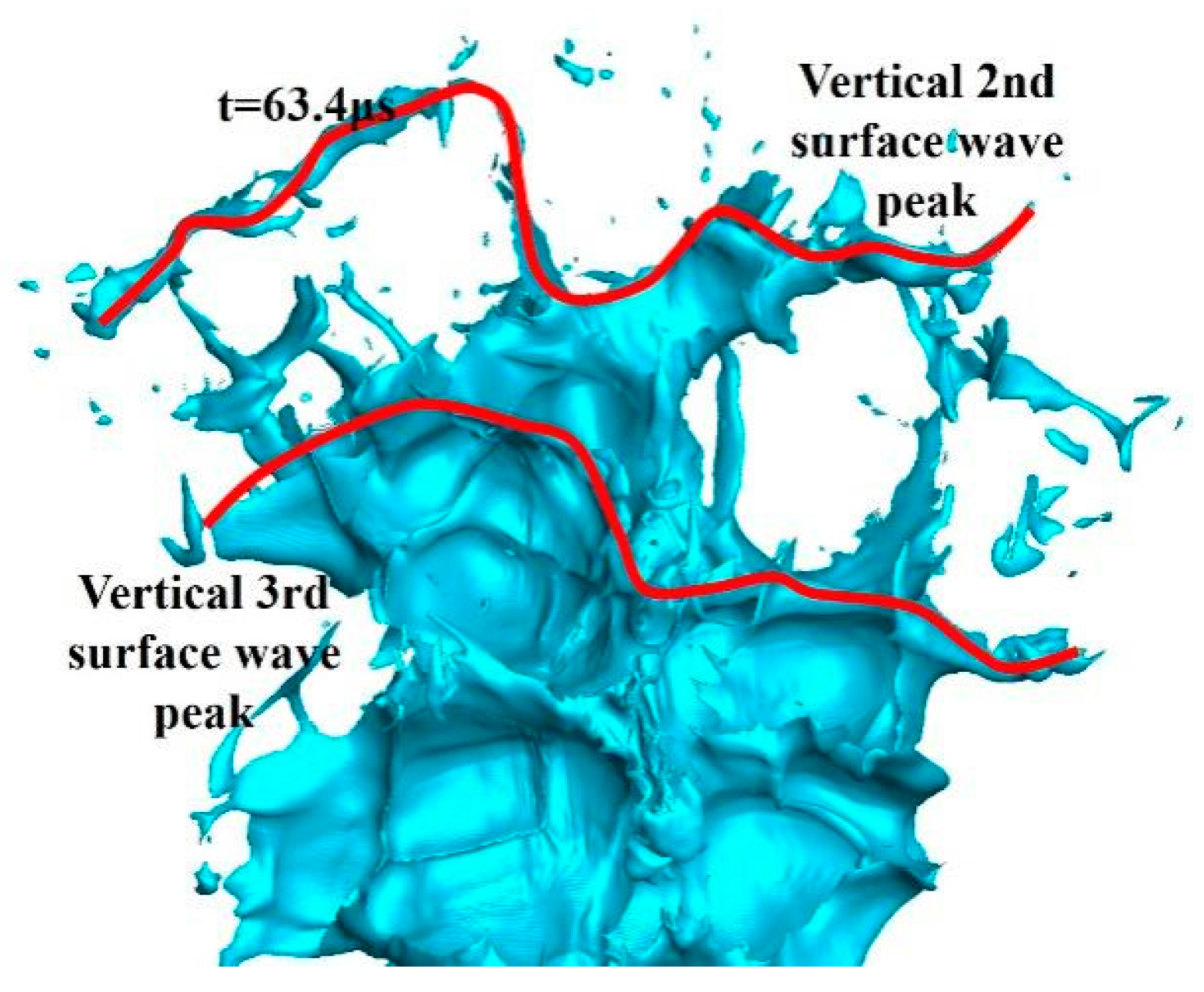
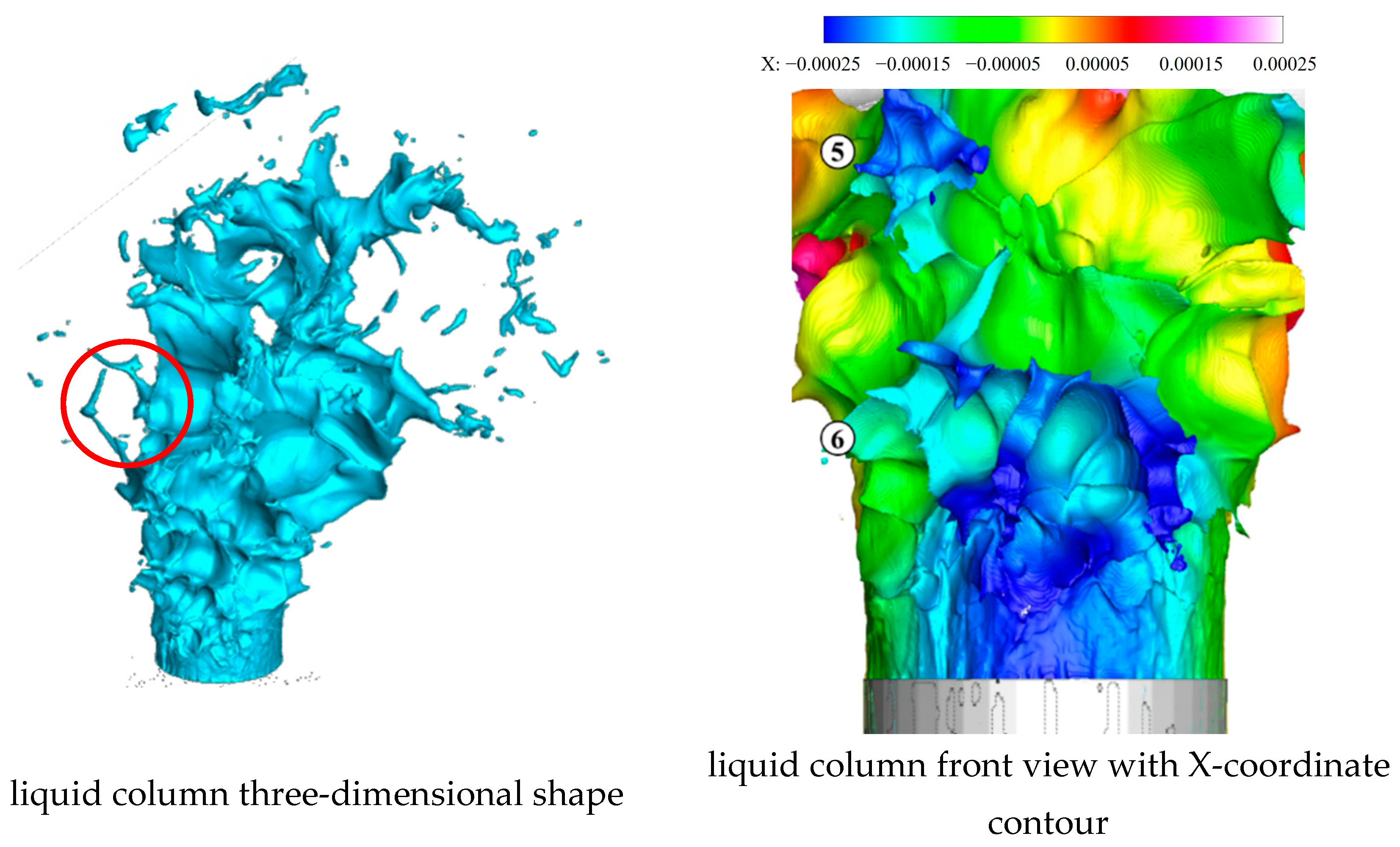
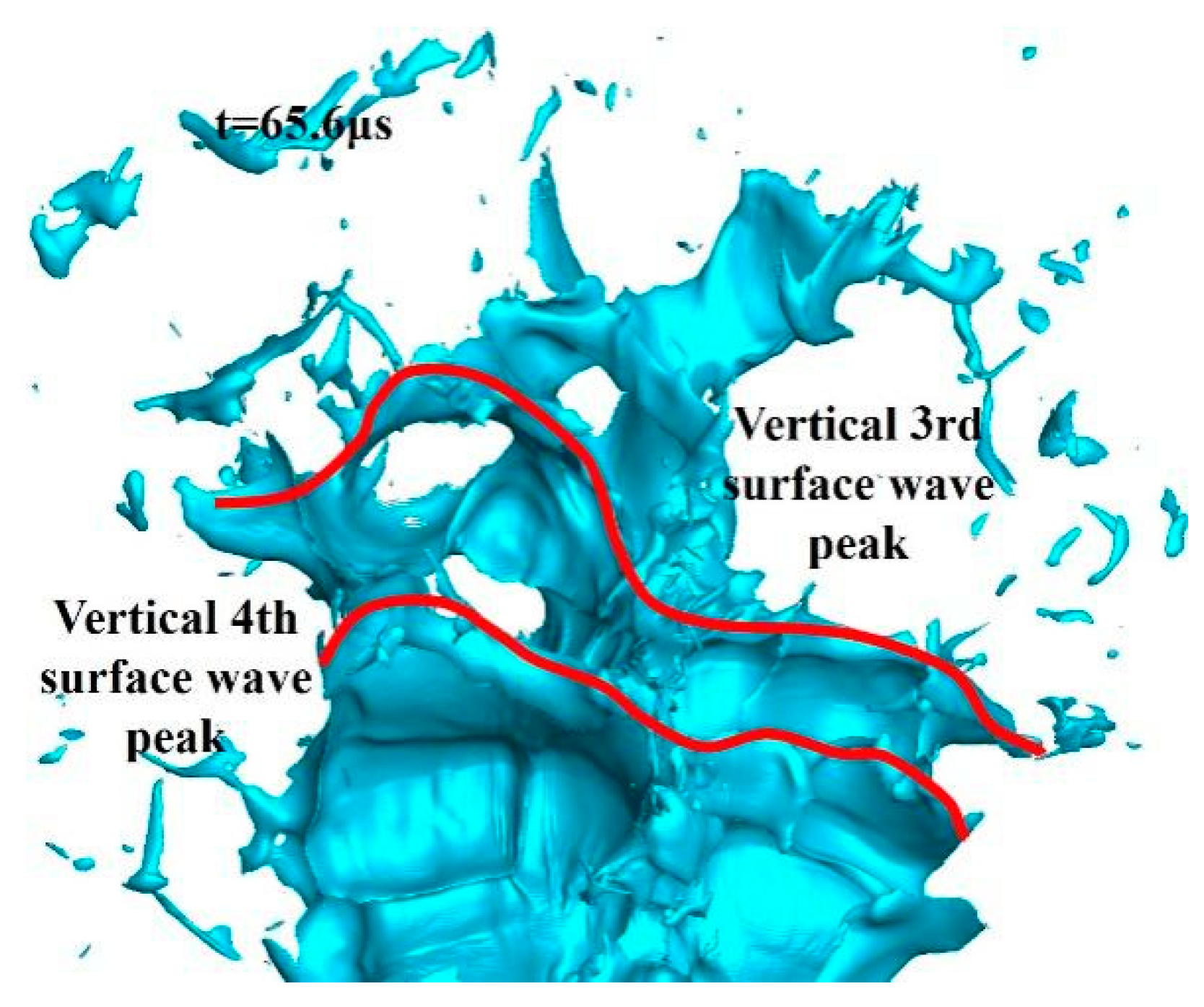
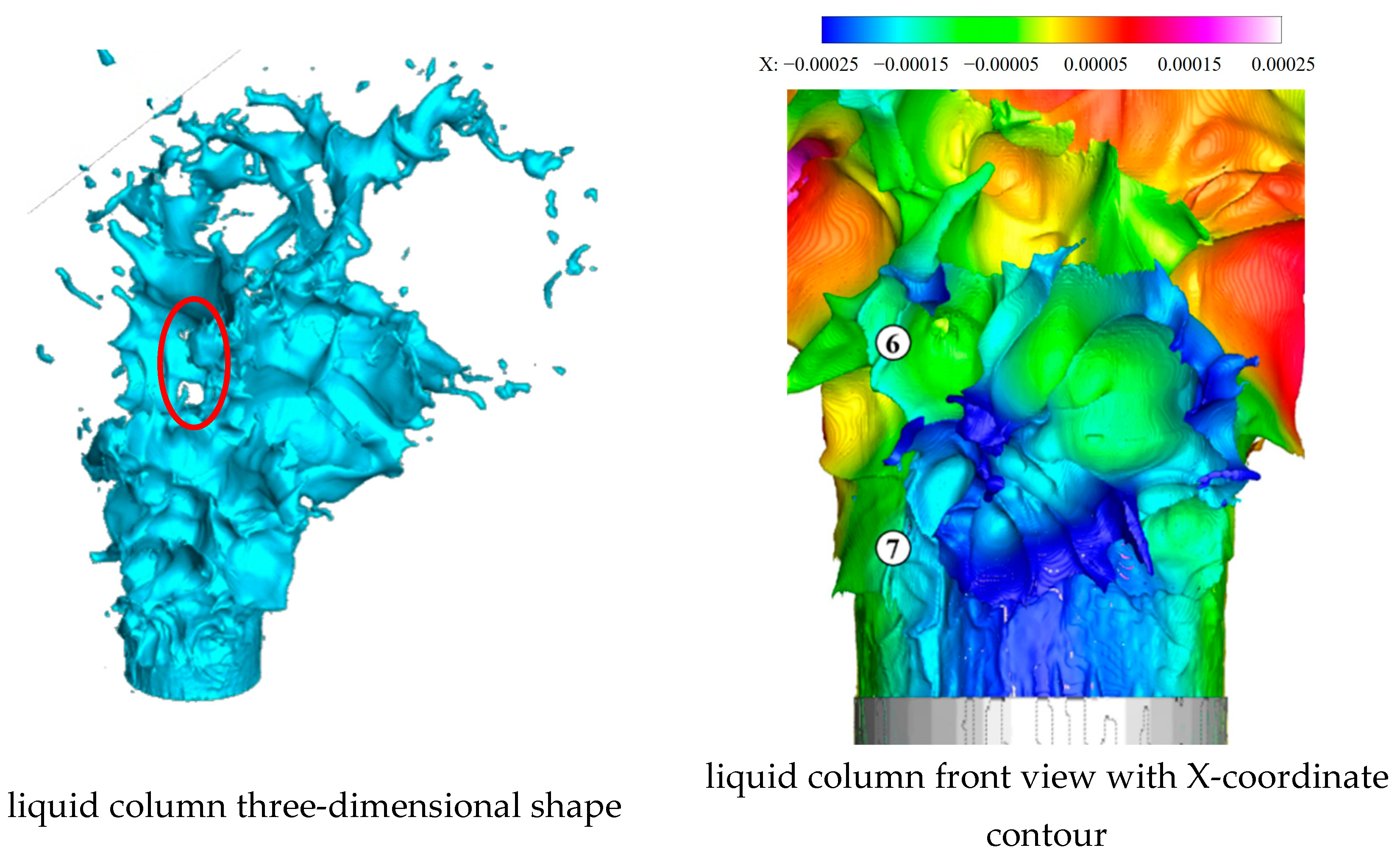
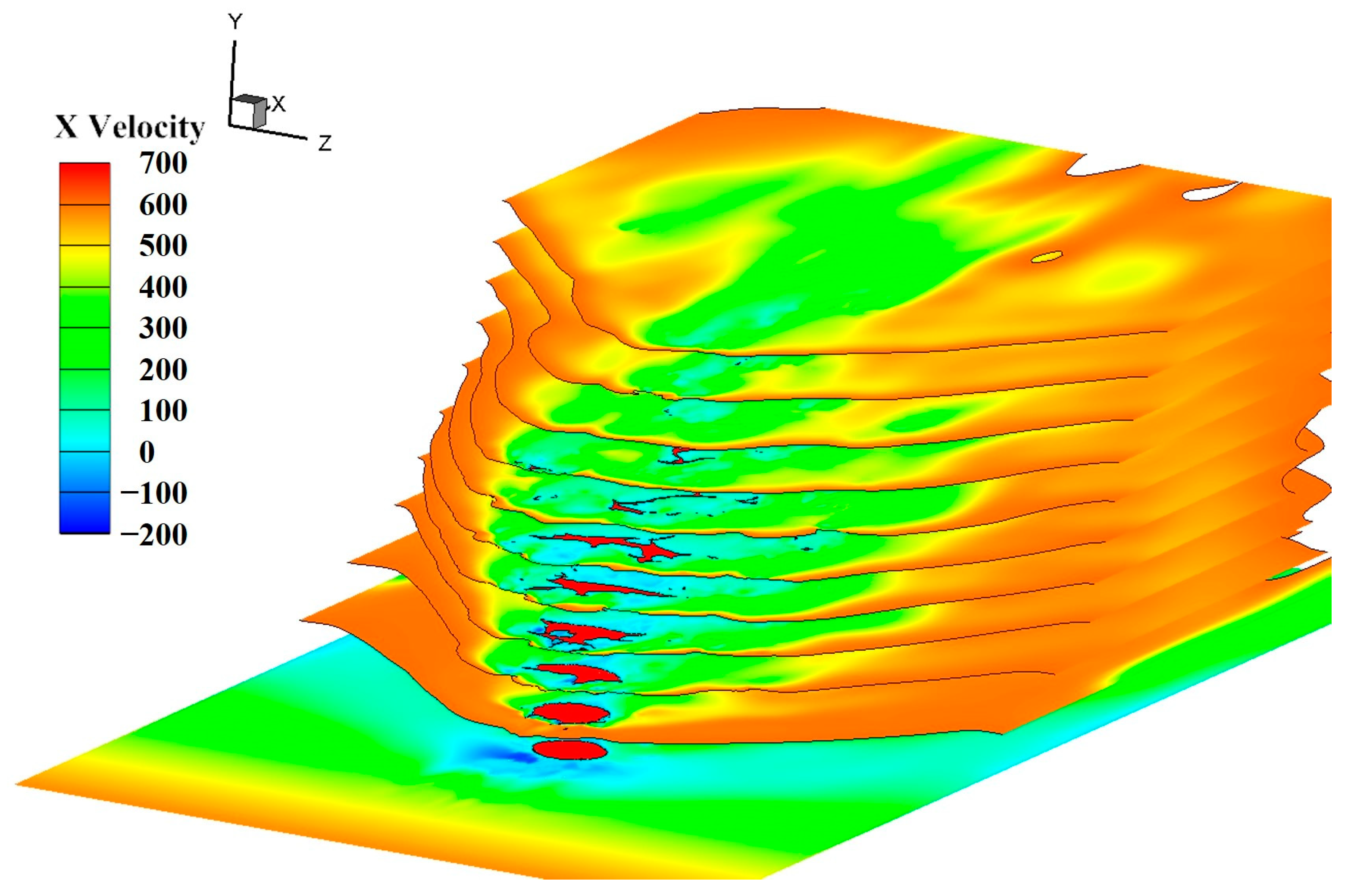
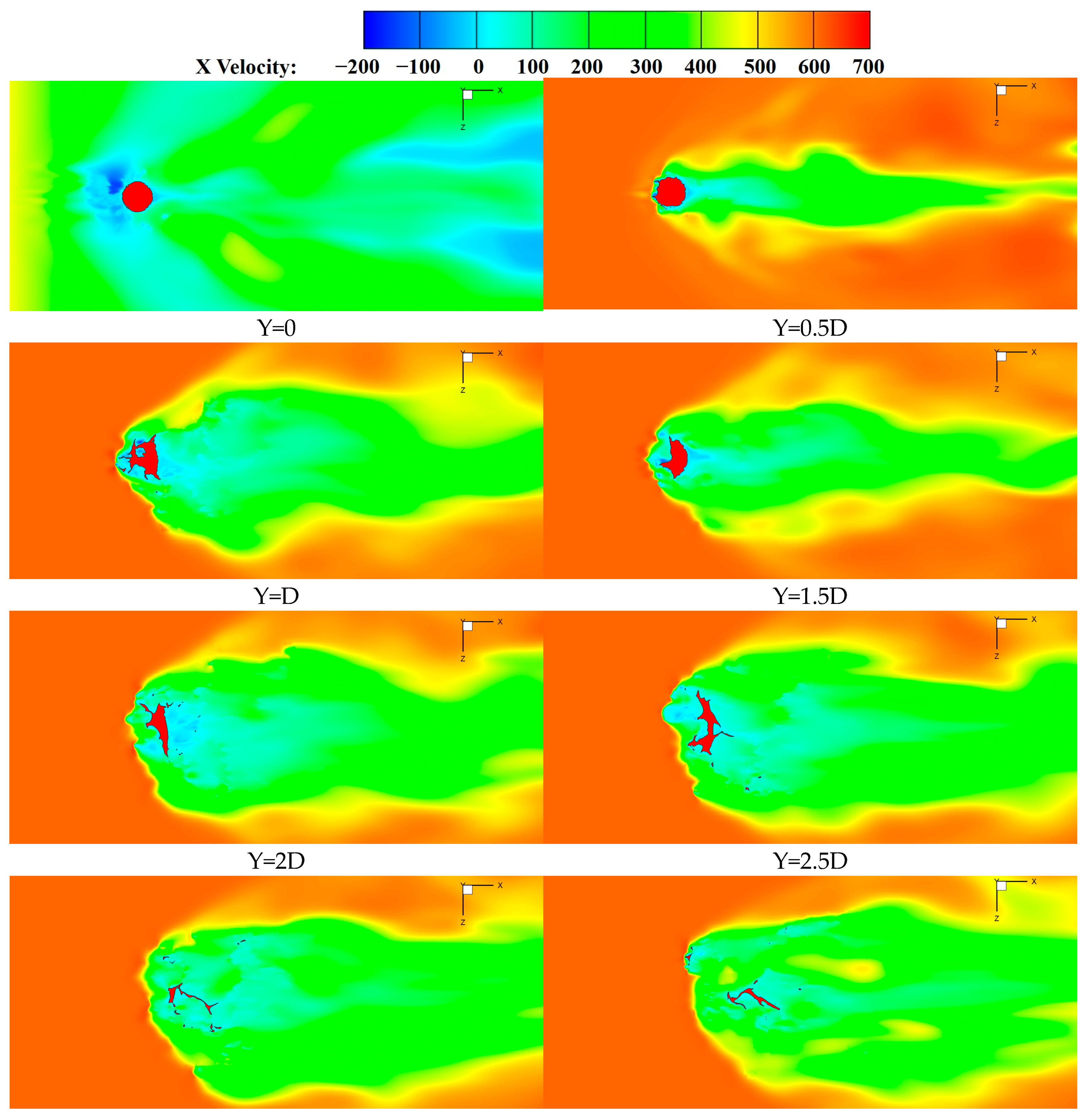
3.2.2. Vertical Flow Field Analysis of Supersonic LJIC

Figure 43 shows the evolution process of the X-direction velocity contour and the Mach number contour of the flow field from 41.0 μs to 80.2 μs, in which the red part represents the liquid jet and the black line in the Mach number contour on the right is the isoline at Ma = 1. Comparing the X-direction velocity with the Mach number, the distributions of both are always similar. In most areas above the liquid column that are hardly affected by the jet, the X-direction velocity and Mach number are relatively stable, whose values are the initial set values of the crossflow (the initial X-direction velocity is 611 m/s and the initial Mach number is 2.85).

In the X-direction velocity contour, due to the obstruction effect of the liquid column, the crossflow sharply slows down, bypasses the liquid column at a low speed to reach the leeward side, and then accelerates again. The crossflow decelerates rapidly at the jet’s windward side but accelerates slowly at the jet’s leeward side, resulting in a short distance from the bow shock wave to the jet and a long, low-speed area behind the jet. Above the jet, the crossflow area, whose velocity is affected by the jet, becomes larger gradually and extends diagonally upwards with the development of the jet. There is a negative flow velocity region in the near-wall region ahead of the jet, which is located between the bow shock wave and the separation shock wave, called the separation zone or reflux zone. Taking 59.4 μs as an example, the overall and local streamline contours are shown in Figure 44. The stagnation of the airflow ahead of the liquid column leads to the formation of a local high-pressure zone, where a reverse pressure gradient is generated and propagates upstream through the subsonic zone of the boundary layer. Due to the airflow reflux, a local subsonic zone is generated, which causes a certain distance from the bow shock wave’s starting point to the wall. In the separation zone, the upper airflow flows forward, while the near-wall airflow flows in the opposite direction, forming a circular airflow, as shown in the red arrow of Figure 44.

The black line in the Mach number contour on the right is the isoline at Ma = 1. The Mach number of the airflow in the separation zone gradually decreases along the flow direction. The crossflow ahead of the liquid column undergoes a violent deceleration after passing through the bow shock wave, resulting in a short subsonic region. The acceleration process of the airflow behind the liquid column is relatively mild and the speed increases slowly, resulting in a relatively long subsonic region behind the jet. In the jet development process, the subsonic region changes from being close to the wall to leaving the wall, and continuously expanding vertically. This is because, as the jet deepens into the crossflow, the width of the jet’s windward surface continues to increase, the aerodynamic force acting on the liquid column continues to expand in a spanwise direction, and the obstruction effect of the liquid column on the crossflow continues to increase.

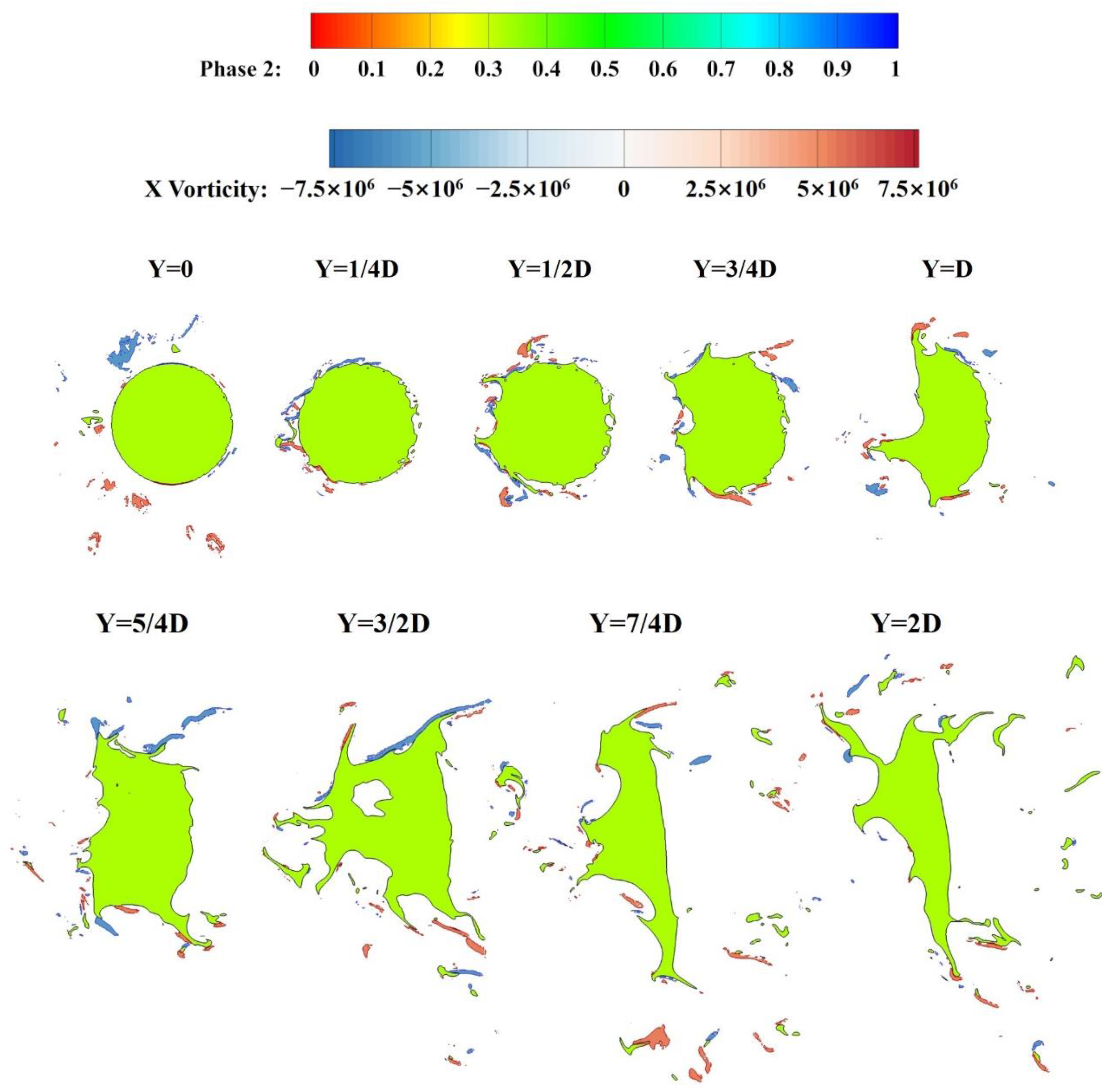
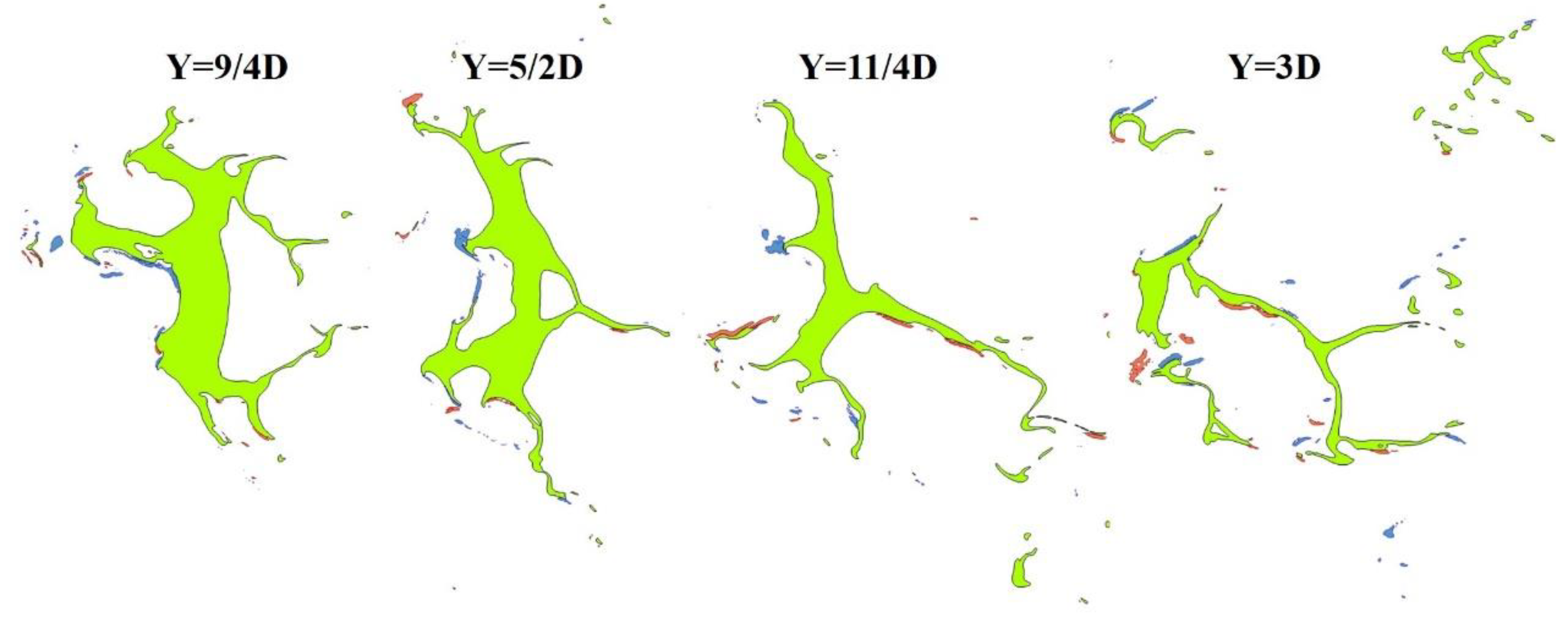
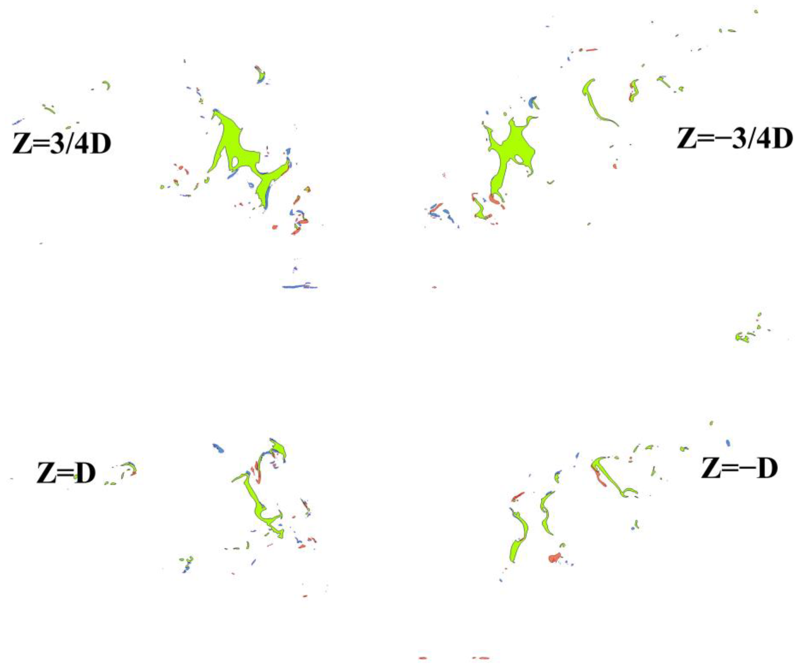
3.2.3. Spanwise Flow Field Analysis of Supersonic LJIC

The relative positions of the X-direction velocity contour on 11 vertical sections at 80.2 μs are shown in Figure 45. The flow field at 80.2 μs is fully developed and representative. The contours on each section are shown in Figure 46.

The X-direction velocity contours of 11 vertical sections from Y = 0 to Y = 5D are shown in Figure 46, where the black curve represents the gas–liquid interface and the red part in the black curve represents the liquid phase of the corresponding section.

The description of the liquid phase in the vertical section is as follows: The liquid column at the wall (Y = 0), whose shape is circular, has not yet been affected by the crossflow. As the section moves upwards (Y = 0.5D), the varying degrees of spanwise surface waves are generated around the liquid column. Between the section of Y = 1D and 1.5D, a hole that has evolved from the surface wave inside the liquid column is generated and subsequently fragmented. Afterward, the shape of the liquid phase gradually becomes thinner in the crossflow direction and longer in the spanwise direction, and this tendency becomes more and more obvious thereafter. At the Y = 3D section, most of the jet has already disintegrated, with only residual slender strip structures corresponding to the three-dimensional liquid film. The liquid structure at Y = 4D to 5D has disintegrated completely.

The description of the gas phase in the vertical section is as follows: The velocity of the Y = 0 section is generally low due to the wall boundary layer, and the crossflow upstream velocities on all other sections are the same, which is the initial crossflow velocity. A blue separation zone ahead of the liquid column, accompanied by obvious wake zones on both sides, can be seen on the Y = 0 section. Starting from the Y = 0.5D section, it can be seen that there are obvious low-speed zones within a short distance on the windward side and both sides of the liquid column, as well as in the larger area on the leeward side of the liquid column. The transition between the upstream low-speed zone and the high-speed zone is the location of the bow shock wave. However, the overall velocity is subsonic due to the boundary layer at Y = 0 section and there are no shock waves, due to the incompressibility of subsonic flow. It can also be observed that the shock wave standoff distance, the distance between the liquid column and the bow shock wave gradually increases. The spanwise span of the low-speed region shows an increasing trend, because the liquid column cross-section spanwise length and the liquid phase area that hinders the crossflow increase with the increase in the vertical direction. In the range of Y = 4D to 5D, the disintegration of the liquid column is almost completed and there is little liquid phase left, while the jet still impacts the crossflow and the bow shock wave’s spanwise span shows a decreasing trend. Few momentum exchanges occur between the jet and crossflow in the range of Y = 0.5D to 1D, so the liquid column and bow shock wave hardly move downstream within this range, resulting in an almost vertical liquid column and a normal shock wave. A relatively significant downstream movement of the liquid column and bow shock wave can be observed in the sections above Y = 1D, which is because the momentum exchange between the jet and the crossflow increases, the jet velocity in the crossflow direction increases, the liquid column deflects, and the standoff shock wave moves accordingly.

3.3. Vortex Ring Flow Characteristics of Supersonic LJIC

The vortices influence gas–liquid mixing dramatically, so investigating the vortex ring characteristics is of guiding significance for applications such as fuel combustion and jet control in scramjets. A detailed analysis is conducted on the simulated vortex ring characteristics in this section, which reveals the vortex ring characteristics deeply.

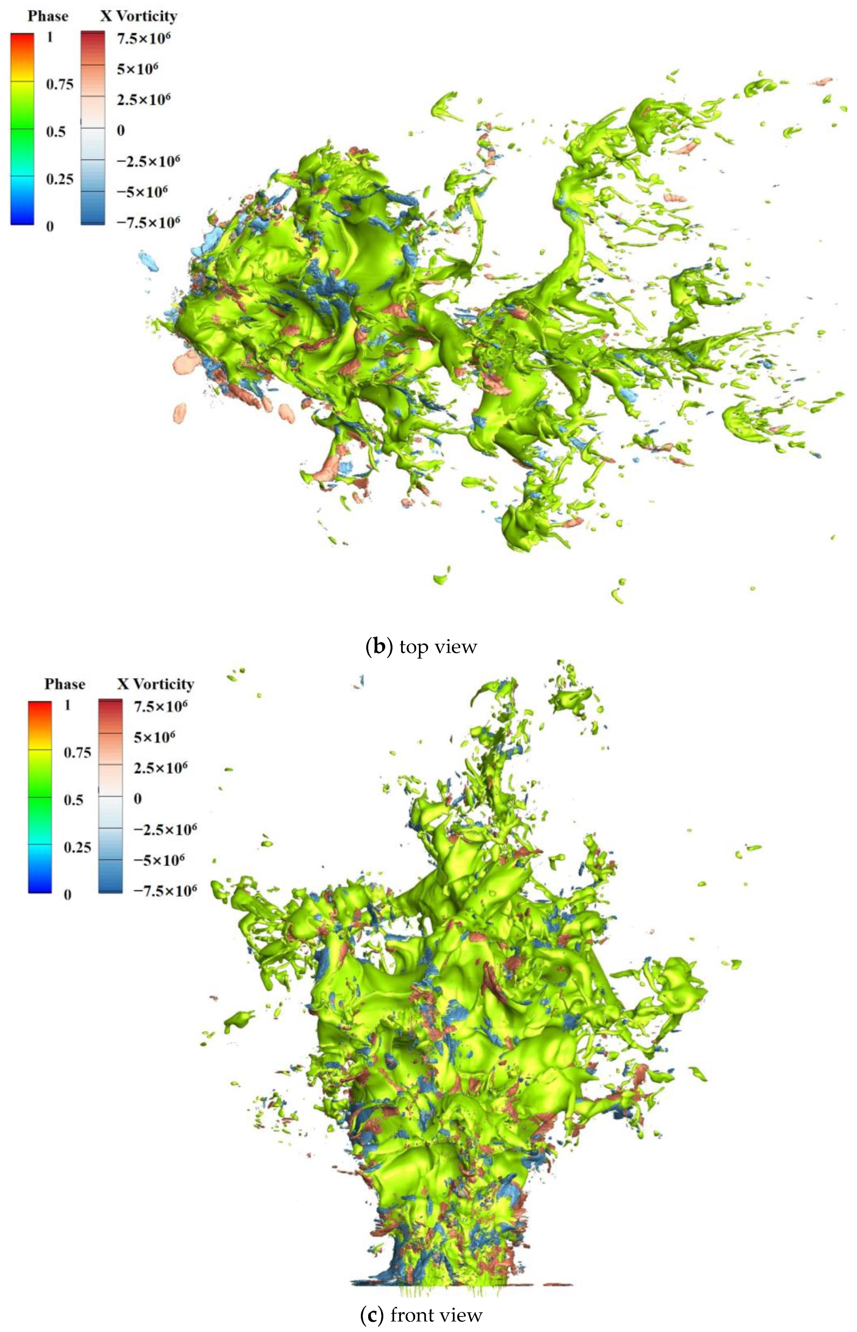
3.3.1. Three-Dimensional Vortex Ring of Supersonic LJIC

The flow characteristics of the vortex ring during the breakup process will be analyzed in this section. Figure 47 shows the side view, top view, front view, and rear view of the liquid column and the X-vorticity isosurfaces of ±5,000,000, where the liquid column is light green, the positive vorticity is red, and the negative is blue.

The distribution of vortices is very extensive, with a dense distribution in the side, top, and front areas. From the side view, it can be seen that there are large vortices on both sides of the liquid column, especially near the inlet, where the liquid column deforms little. It can be seen that the vortices are intensive and small-sized on the liquid column’s windward side from the top and front views. On the liquid column’s windward side, the gas–liquid interaction is strong and the airflow state is complex and variable, leading to a numerous and dense vortex distribution characteristic. In the rearview, the vortices are distributed sparsely, especially at the smooth leeward surface of the liquid column.

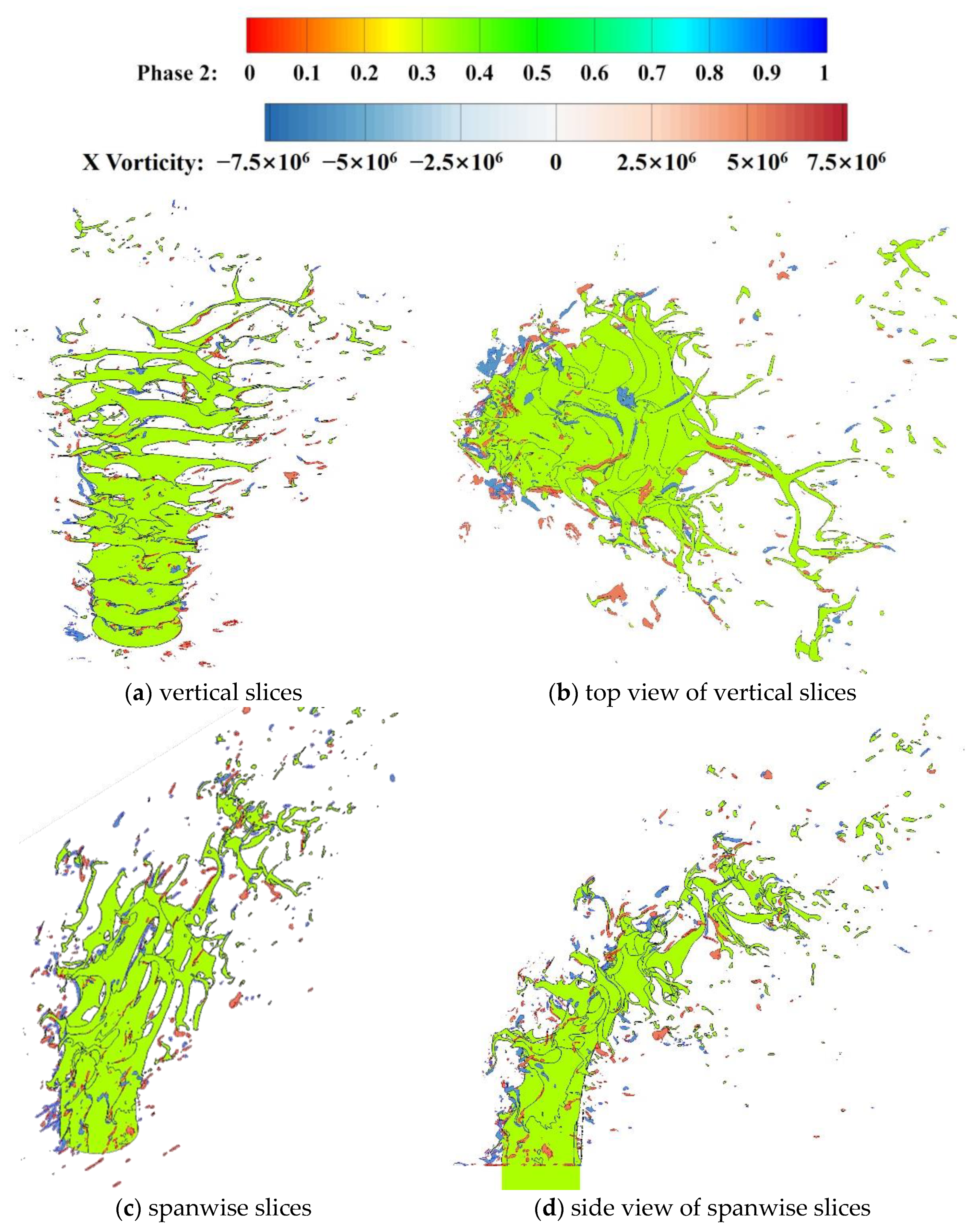
3.3.2. Vortex Ring Flow Characteristics of Supersonic LJIC

The morphology of the liquid column during the breakup process is complex and it is difficult to achieve intuitive results by analyzing the three-dimensional liquid column and vortex ring directly. Therefore, multiple vertical and spanwise two-dimensional slices of the liquid column and X-vortex ring will be analyzed in this section. The liquid phase and X-vorticity contour on the sections are plotted on 13 sections from Y = 0 to Y = 3D and 9 sections from Z = −D to Z = D, where red is positive and blue is negative. Figure 48 shows the relative position schematic diagram and top view of the vertical and spanwise sections.

Figure 49 shows the isolines of the liquid phase and X-vorticity at 13 cross-sections between Y = 0 and Y = 3D. It can be seen that the vortices are mostly attached to the protruding structures of the liquid column section, which is the spanwise surface wave peak. The vortices at the wall are far away from the liquid column due to the separation zone. The vortices are distributed uniformly and symmetrically from Y = 1/4D to Y = 1/2D, because the liquid column here deforms less and remains circular, and the airflow here flows regularly. Between the Y = 3/4D and Y = D sections, the liquid column becomes elliptical, and obvious spanwise surface waves appear on the liquid column’s windward side. And there are vortices at the peak of the spanwise surface wave, while there are fewer vortices at the valley. In the range of Y = 5/4D to Y = 2D, the cross-section of the liquid column becomes thinner in the flow direction and longer in the spanwise direction, and some droplets fall off. It can be observed that there are obvious wake vortices on both sides of the liquid column, which is due to the strong shear effect between the thinner liquid column and the crossflow. There are also vortices around droplets that have fallen off. Between Y = 9/4D and Y = 3D, the liquid column has undergone severe deformation into a thin liquid film, and vortices mainly exist ahead of the protrusion structure of the liquid film’s windward side and the strip structure on the liquid film’s leeward side.

Figure 50 shows the isolines of the liquid phase and X-vorticity at nine cross-sections between Z = −D and Z = D. The vortex characteristics will be analyzed from a spanwise perspective. On the Z = 0 and Z = ±1/4D sections, at the position where the liquid column is close to the injection nozzle without significant deflection, the airflow is nearly perpendicular to the liquid column, and vortices are mostly distributed at the peaks of the vertical surface wave. At the upper position of the liquid column, the liquid column has undergone significant deflection and breakup, with vortices mostly distributed at the large valleys of the vertical surface wave. And clear wake vortices can be observed at the large droplets that have already fallen off. On the Z = ±1/2D section, the liquid column’s spanwise width increases here compared to the inlet. The liquid phase section, below which is the airflow, is not connected to the wall. There are multiple obvious vortices below the liquid phase due to the jet–crossflow shear effects. Such a situation where vortices concentrate in a certain area is special, mainly because the liquid column starts to extend and is close to the liquid column here. The region of Z = ±3/4D to Z = ±D is relatively far away from the liquid column compared to the Z = ±1/2D section, and the spanwise development is more complete. The vortices here mainly extend from the multi-vortex concentration area below the Z = ±1/2D section, as well as the wake vortices on the upper and lower sides of the jet–crossflow shear position.

4. Conclusions

The breakup process, atomization mechanism, flow field characteristics, and vortex ring flow characteristics of supersonic LJIC primary atomization were investigated in this study, and the conclusions are as follows:

(1) Under the current simulation conditions, surface waves on the liquid column’s windward surface exist in a two-dimensional method, including vertical and spanwise surface waves. The interaction between such two kinds of surface waves results in crisscrossed peaks and valleys on the liquid column’s windward surface. The column breakup occurs only when all spanwise surface waves between adjacent vertical surface waves are broken. And shear breakup occurs on both sides of the liquid column.

(2) The supersonic LJIC flow field contains characteristics such as bow shock waves, secondary shock waves, and separation zones. The bow shock wave, whose shape changes with the change in the surface wave shape, is composed of multiple connected arc-shaped shock waves.

(3) The vortex ring flow characteristics of supersonic LJICs are relatively complex, which differ in various spanwise and vertical cross-sections.

In the combustion chamber of scramjets, how to promote and enhance fuel–air mixing in a short time is a major challenge in supersonic combustion. In this manuscript, the supersonic LJIC characteristics, including the breakup process, flow field characteristics, and vortex characteristics, are investigated deeply. Through this, our understanding of LJICs can be deepened and a more effective atomization effect can be achieved in subsequent research, thereby improving combustion efficiency.

However, there are still some limitations to this study, which are as follows:

(1) The analysis of the flow field and vortex fields should be enriched. For example, the proper orthogonal decomposition (POD) can be employed in the research.

(2) The flow characteristics of LJICs should be investigated using comparative verification, which is mainly based on experimental research supplemented with numerical simulation.

(3) Different injection nozzle shapes, injection angles, and pulsed jets should be studied to comprehensively reveal the flow mechanism and influencing factors of LJICs, which is also the direction of our next work.

(4) There is little research on the relationship between the atomization characteristics and the vortex flow characteristics. The proposal and resolution of these issues are crucial for our research and exploration of the atomization of liquid fuels in supersonic transverse airflow.

References

1. Li, C.; Zhou, Y.; Chen, H.; Li, Q. Cross-sectional droplets distribution of a liquid jet in supersonic crossflow. Acta Astronaut. 2021, 186, 109–117. [Google Scholar] [CrossRef]
2. Wang, Z.-G.; Wu, L.; Li, Q.; Li, C. Experimental investigation on structures and velocity of liquid jets in a supersonic crossflow. Appl. Phys. Lett. 2014, 105, 134102. [Google Scholar] [CrossRef]
3. Li-Yin, W.; Zhen-Guo, W.; Qing-Lian, L.; Chun, L. Unsteady oscillation distribution model of liquid jet in supersonic crossflows. Acta Phys. Sin. 2016, 65, 186–194. [Google Scholar] [CrossRef]
4. Wu, L.; Zhang, K.; Li, C.; Li, Q. Model for three-dimensional distribution of liquid fuel in supersonic cross-flows. J. Exp. Fluid Mech. 2018, 32, 20–30. [Google Scholar]
5. Wu, L.; Wang, Z.-G.; Li, Q.; Zhang, J. Investigations on the droplet distributions in the atomization of kerosene jets in supersonic crossflows. Appl. Phys. Lett. 2015, 107, 104103. [Google Scholar] [CrossRef]
6. Yang, H.; Li, F.; Sun, B. Trajectory analysis of fuel injection into supersonic cross flow based on schlieren method. Chin. J. Aeronaut. 2012, 25, 42–50. [Google Scholar] [CrossRef]
7. Nambu, T.; Mizobuchi, Y. Detailed numerical simulation of primary atomization by crossflow under gas turbine engine com-bustor conditions. Proc. Combust. Inst. 2021, 38, 3213–3221. [Google Scholar] [CrossRef]
8. Behzad, M.; Ashgriz, N.; Karney, B. Surface breakup of a non-turbulent liquid jet injected into a high pressure gaseous crossflow. Int. J. Multiph. Flow 2016, 80, 100–117. [Google Scholar] [CrossRef]
9. Mukundan, A.A.; Tretola, G.; Ménard, T.; Herrmann, M.; Navarro-Martinez, S.; Vogiatzaki, K.; de Motta, J.C.B.; Berlemont, A. DNS and LES of primary atomization of turbulent liquid jet injection into a gaseous crossflow environment. Proc. Combust. Inst. 2021, 38, 3233–3241. [Google Scholar] [CrossRef]
10. Xiao, F.; Dianat, M.; McGuirk, J.J. Large eddy simulation of liquid-jet primary breakup in air crossflow. AIAA J. 2013, 51, 2878–2893. [Google Scholar] [CrossRef]
11. Wen, J.; Hu, Y.; Nakanishi, A.; Kurose, R. Atomization and evaporation process of liquid fuel jets in crossflows: A numerical study using Eulerian/Lagrangian method. Int. J. Multiph. Flow 2020, 129, 103331. [Google Scholar] [CrossRef]
12. Jadidi, M.; Dolatabadi, A. On the trajectory of nonturbulent liquid jets in subsonic crossflows at different density ratios. Theor. Appl. Mech. Lett. 2018, 8, 277–283. [Google Scholar] [CrossRef]
13. Zhao, J.; Yan, C.; Wu, L.; Lin, W.; Tong, Y.; Nie, W. Numerical simulation of single/double liquid jets in supersonic crossflows. Aerosp. Sci. Technol. 2022, 120, 107289. [Google Scholar] [CrossRef]
14. Xiao, F.; Wang, Z.G.; Sun, M.B.; Liang, J.H.; Liu, N. Large eddy simulation of liquid jet primary breakup in supersonic air crossflow. Int. J. Multiph. Flow 2016, 87, 229–240. [Google Scholar] [CrossRef]
15. Xiao, F.; Sun, M.B. Effects of Mach number on liquid jet primary breakup in gas crossflow. At. Sprays 2018, 28, 975–999. [Google Scholar] [CrossRef]
16. Li, C.; Shen, C.; Li, Q.; Zhu, Y. Primary breakup process of liquid jet in supersonic crossflow. J. Natl. Univ. Def. Technol. 2019, 41, 73–78. [Google Scholar]
17. Zhou, Y.; Li, Q.; Li, C. Study on Breaking Process of Liquid Jet in Supersonic Flow Based on Adaptive Mesh. J. Propuls. Technol. 2020, 41, 1571–1579. [Google Scholar]
18. Li, P.; Wang, Z.; Sun, M.; Wang, H. Numerical simulation of the gas-liquid interaction of a liquid jet in supersonic crossflow. Acta Astronaut. 2017, 134, 333–344. [Google Scholar] [CrossRef]
19. Li, P.; Wang, Z.; Bai, X.-S.; Wang, H.; Sun, M.; Wu, L.; Liu, C. Three-dimensional flow structures and droplet-gas mixing process of a liquid jet in supersonic crossflow. Aerosp. Sci. Technol. 2019, 90, 140–156. [Google Scholar] [CrossRef]
20. Li, P.; Wang, Z.; Sun, M.; Wang, H. Numerical Simulation of the Gas-Liquid Interaction of Cross Liquid Jet in Supersonic Flow. J. Astronaut. 2016, 37, 209–215. [Google Scholar]
21. Liu, W.L.; Zhu, L.; Qi, Y.Y.; Ge, J.R.; Luo, F.; Zou, H.R.; Wei, M.; Jen, T.C. Effects of injection pressure variation on mixing in a cold supersonic combustor with kerosene fuel. Acta Astronaut. 2017, 139, 67–76. [Google Scholar] [CrossRef]
22. Zhu, L.; Luo, F.; Qi, Y.-Y.; Wei, M.; Ge, J.-R.; Liu, W.-L.; Li, G.-L.; Jen, T.-C. Effects of spray angle variation on mixing in a cold supersonic combustor with kerosene fuel. Acta Astronaut. 2018, 144, 1–11. [Google Scholar] [CrossRef]
23. Zhu, L.; Qi, Y.Y.; Liu, W.L.; Xu, B.J.; Ge, J.R.; Xuan, X.C.; Jen, T.C. Numerical investigation of scale effect of various injection diameters on interaction in cold ker-osene-fueled supersonic flow. Acta Astronaut. 2016, 129, 111–120. [Google Scholar] [CrossRef]
24. Zhou, Y.-Z.; Xiao, F.; Li, Q.-L.; Li, C.-Y. Simulation of elliptical liquid jet primary breakup in supersonic crossflow. Int. J. Aerosp. Eng. 2020, 2020, 1–12. [Google Scholar] [CrossRef]
25. Niu, Y.Y.; Wu, C.H.; Huang, Y.H.; Chou, Y.J.; Kong, S.C. Evaluation of breakup models for liquid side jets in supersonic cross flows. Numer. Heat Transf. Part A Appl. 2020, 79, 353–369. [Google Scholar] [CrossRef]
26. Almanzalawy, M.S.; Rabie, L.H.; Mansour, M.H. Modeling of an efficient airblast atomizer for liquid jet into a supersonic crossflow. Acta Astronaut. 2020, 177, 142–157. [Google Scholar] [CrossRef]
27. Zhu, Y.H.; Xiao, F.; Li, Q.L.; Mo, R.; Li, C.; Lin, S. LES of primary breakup of pulsed liquid jet in supersonic crossflow. Acta Astronaut. 2019, 154, 119–132. [Google Scholar] [CrossRef]
28. Liu, N.; Wang, Z.; Sun, M.; Deiterding, R.; Wang, H. Simulation of liquid jet primary breakup in a supersonic crossflow under Adaptive Mesh Refinement framework. Aerosp. Sci. Technol. 2019, 91, 456–473. [Google Scholar] [CrossRef]
29. Allaire, G.; Clerc, S.; Kokhc, S. A five-equation model for the simulation of interfaces between compressible fluids. J. Comput. Phys. 2002, 181, 577–616. [Google Scholar] [CrossRef]
30. Lin, S.; Shen, C.; Xiao, F.; Zhu, Y. Large Eddy Simulation of Primary Breakup of Transverse Pulsed Liquid Jet in Supersonic Flow. J. Combust. Sci. Technol. 2020, 26, 87–95. [Google Scholar]
31. Hu, R.; Li, Q.; Li, C.; Li, C. Effects of an accompanied gas jet on transverse liquid injection in a supersonic crossflow. Acta Astronaut. 2019, 159, 440–451. [Google Scholar] [CrossRef]
32. Zhao, J.; Lin, W.; Yan, C.; Zheng, Z.; Tong, Y.; Nie, W. Mixing enhancement mechanism of combined H2–Water jets in supersonic crossflows in a com-bustor with an expanded section. Int. J. Hydrog. Energy 2022, 47, 10747–10761. [Google Scholar] [CrossRef]
33. Zhao, J.; Nie, W.; Tong, Y.; Ren, Y.; Zhu, Y.; Lin, W. Effects of Injection Angles on Liquid Jets in Supersonic Crossflows. J. Propuls. Technol. 2022, 43, 239–249. [Google Scholar]
34. Almeida, H.; Sousa, J.M.M.; Costa, M. Effect of the liquid injection angle on the atomization of liquid jets in subsonic crossflows. At. Sprays 2014, 24, 81–96. [Google Scholar] [CrossRef]
35. Beloki Perurena, J.; Asma, C.O.; Theunissen, R.; Chazot, O. Experimental investigation of liquid jet injection into Mach 6 hypersonic crossflow. Exp. Fluids 2009, 46, 403–417. [Google Scholar] [CrossRef]
36. Olyaei, G.; Kebriaee, A. Experimental study of liquid jets injected in crossflow. Exp. Therm. Fluid Sci. 2020, 115, 110049. [Google Scholar] [CrossRef]
37. Jadidi, M.; Sreekumar, V.; Dolatabadi, A. Breakup of elliptical liquid jets in gaseous crossflows at low Weber numbers. J. Vis. 2019, 22, 259–271. [Google Scholar] [CrossRef]
38. Prakash, R.S.; Sinha, A.; Tomar, G.; Ravikrishna, R. Liquid jet in crossflow—Effect of liquid entry conditions. Exp. Therm. Fluid Sci. 2018, 93, 45–56. [Google Scholar] [CrossRef]
39. Lee, I.C.; Kang, Y.S.; Moon, H.J.; Jang, S.P.; Kim, J.K.; Koo, J. Spray jet penetration and distribution of modulated liquid jets in subsonic cross-flows. J. Mech. Sci. Technol. 2010, 24, 1425–1431. [Google Scholar] [CrossRef]
40. Lee, I.; Kang, Y.; Koo, J. Mixing characteristics of pulsed air-assist liquid jet into an internal subsonic cross-flow. J. Therm. Sci. 2010, 19, 136–140. [Google Scholar] [CrossRef]
41. Sussman, M.; Puckett, E.G. A coupled level set and volume-of-fluid method for computing 3D and axisymmetric incompressible two-phase flows. J. Comput. Phys. 2000, 162, 301–337. [Google Scholar] [CrossRef]
42. Xiao, F.; Wang, Z.G.; Sun, M.B.; Liang, J.H.; Liu, N. Large Eddy Simulation of Droplet Breakup in Supersonic Flow. J. Propuls. Technol. 2016, 37, 706–712. [Google Scholar]
43. Smagorinsky, J. General circulation experiments with the primitive equations: I. The basic experiment. Mon. Weather Rev. 1963, 91, 99–164. [Google Scholar] [CrossRef]
44. Deardorff, J.W. A numerical study of three-dimensional turbulent channel flow at large Reynolds numbers. J. Fluid Mech. 1970, 41, 453–480. [Google Scholar] [CrossRef]
45. Scotti, A.; Meneveau, C.; Lilly, D.K. Generalized Smagorinsky model for anisotropic grids. Phys. Fluids A Fluid Dyn. 1993, 5, 2306–2308. [Google Scholar] [CrossRef]
46. Moeng, C.H.; Wyngaard, J.C. Spectral analysis of large-eddy simulations of the convective boundary layer. J. Atmos. Sci. 1988, 45, 3573–3587. [Google Scholar] [CrossRef]
47. Fuster, D.; Agbaglah, G.; Josserand, C.; Popinet, S.; Zaleski, S. Numerical simulation of droplets, bubbles and waves: State of the art. Fluid Dyn. Res. 2009, 41, 065001. [Google Scholar] [CrossRef]
48. Sussman, M.; Almgren, A.S.; Bell, J.B.; Colellab, P.; Howell, L.H.; Welcome, M.L. An Adaptive Level Set Approach for Incompressible Two-Phase Flows. J. Comput. Phys. 1999, 148, 81–124. [Google Scholar] [CrossRef]
49. Lebas, R.; Menard, T.; Beau, P.; Berlemont, A.; Demoulin, F. Numerical simulation of primary break-up and atomization: DNS and modelling study. Int. J. Multiph. Flow 2009, 35, 247–260. [Google Scholar] [CrossRef]
Figure 1. Flow field structure of a supersonic LJIC.
Aerospace 10 00995 g001
Figure 2. Computational domain.
Aerospace 10 00995 g002
Figure 3. CLSVOF process.
Aerospace 10 00995 g003
Figure 4. Meshes with different levels.
Aerospace 10 00995 g004
Figure 5. Y-direction velocity calculation results at the symmetry plane of Level 3, Level 4, and Level 5 AMR.
Aerospace 10 00995 g005
Figure 6. Comparison of penetration result with Li [16].
Aerospace 10 00995 g006
Figure 7. Evolution process of the jet.
Aerospace 10 00995 g007
Figure 8. Sketch map of the method of coloring the jet with X-coordinate contours.
Aerospace 10 00995 g008
Figure 9. Liquid column at 35.7 μs.
Aerospace 10 00995 g009
Figure 10. Liquid column at 38.5 μs.
Aerospace 10 00995 g010
Figure 11. Liquid column at 41.0 μs.
Aerospace 10 00995 g011
Figure 12. Liquid column at 43.6 μs.
Aerospace 10 00995 g012
Figure 13. Liquid column at 45.5 μs.
Aerospace 10 00995 g013
Figure 14. Liquid column at 47.4 μs.
Aerospace 10 00995 g014
Figure 15. Liquid column at 49.5 μs.
Aerospace 10 00995 g015
Figure 16. Liquid column at 51.4 μs.
Aerospace 10 00995 g016
Figure 17. Liquid column at 53.4 μs.
Aerospace 10 00995 g017
Figure 18. The local development trend of the 2nd vertical surface wave peak from 53.4 μs to 55.4 μs.
Aerospace 10 00995 g018
Figure 19. Liquid column at 55.4 μs.
Aerospace 10 00995 g019
Figure 20. Liquid column at 57.3 μs.
Aerospace 10 00995 g020
Figure 21. Liquid column at 59.4 μs.
Aerospace 10 00995 g021
Figure 22. Local liquid column at 59.4 μs.
Aerospace 10 00995 g022
Figure 23. Liquid column at 61.6 μs.
Aerospace 10 00995 g023
Figure 24. Local liquid column at 61.6 μs.
Aerospace 10 00995 g024
Figure 25. Liquid column at 63.4 μs.
Aerospace 10 00995 g025
Figure 26. Local liquid column at 63.4 μs.
Aerospace 10 00995 g026
Figure 27. Liquid column at 65.6 μs.
Aerospace 10 00995 g027
Figure 28. Local liquid column at 65.6 μs.
Aerospace 10 00995 g028
Figure 29. Liquid column at 67.9 μs.
Aerospace 10 00995 g029
Figure 30. Local liquid column at 67.9 μs.
Aerospace 10 00995 g030
Figure 31. Liquid column at 70.0 μs.
Aerospace 10 00995 g031
Figure 32. Local liquid column at 70.0 μs.
Aerospace 10 00995 g032
Figure 33. Liquid column at 71.9 μs.
Aerospace 10 00995 g033
Figure 34. Local liquid column at 71.9 μs.
Aerospace 10 00995 g034
Figure 35. Liquid column at 73.9 μs.
Aerospace 10 00995 g035
Figure 36. Local liquid column at 73.9 μs.
Aerospace 10 00995 g036
Figure 37. Liquid column at 76.0 μs.
Aerospace 10 00995 g037
Figure 38. Local liquid column at 76.0 μs.
Aerospace 10 00995 g038
Figure 39. Liquid column at 78.3 μs.
Aerospace 10 00995 g039
Figure 40. Liquid column at 80.2 μs.
Aerospace 10 00995 g040
Figure 41. The diagram of surface wave two-dimensional form.
Aerospace 10 00995 g041
Figure 42. Supersonic LJIC pressure contour evolution process.
Aerospace 10 00995 g042aAerospace 10 00995 g042b
Figure 43. The evolution process of the X-direction velocity contour and Mach number contour of the flow field from 41.0 μs to 80.2 μs.
Aerospace 10 00995 g043aAerospace 10 00995 g043b
Figure 44. The overall and local streamline of the flow field.
Aerospace 10 00995 g044
Figure 45. The relative positions of the X-direction velocity contour on 11 vertical sections.
Aerospace 10 00995 g045
Figure 46. X-direction velocity contour on vertical section.
Aerospace 10 00995 g046aAerospace 10 00995 g046b
Figure 47. Liquid column and the X-vortex isosurfaces of ±5,000,000.
Aerospace 10 00995 g047aAerospace 10 00995 g047bAerospace 10 00995 g047c
Figure 48. Vertical and spanwise slices of the liquid column and X-vortex ring.
Aerospace 10 00995 g048
Figure 49. The isolines of liquid phase and X-vorticity at 13 cross-sections between Y = 0 and Y = 3D.
Aerospace 10 00995 g049aAerospace 10 00995 g049b
Figure 50. The isolines of liquid phase and X-vorticity at 9 cross-sections between Z = −D and Z = D.
Aerospace 10 00995 g050aAerospace 10 00995 g050b