Article

A Dynamic Air Combat Situation Assessment Model Based on Situation Knowledge Extraction and Weight Optimization

Air Force Engineering University, Baqiao District, Xi’an 710043, China
*
Author to whom correspondence should be addressed.
Aerospace 2023, 10(12), 994; https://doi.org/10.3390/aerospace10120994
Submission received: 22 March 2023 / Revised: 25 May 2023 / Accepted: 29 May 2023 / Published: 27 November 2023
(This article belongs to the Section Aeronautics)

Abstract

:
Air combat situation assessment is the basis of target assignment and maneuver decisions. The current air combat situation assessment models, whether nonparametric or parametric, ignore the continuity and timing of situation changes, making the situation assessment results lose tactical significance. Aimed at the shortcomings of current air combat situation assessment, a dynamic air combat situation assessment model based on situation knowledge extraction and weight optimization was proposed by combining a multiple regression model of hidden logic process, a weight optimization model based on grey prospect theory, a weight mapping model based on autoencoder and extreme learning machine (AE-ELM) and an air combat situation characteristic parameter prediction model based on dynamic weight online extreme learning machine (DWOSELM). Firstly, considering the timing and continuity of air combat situation change, a hidden logic process multiple regression model was introduced to realize the segmentation of air combat situation time series data and the extraction of air combat situation primitives. Secondly, the weight optimization method based on grey prospect theory was used to obtain the weight of the evaluation index under different air combat situations. On this basis, the dynamic mapping model between air combat situation characteristic parameters and the weight of index was constructed by using AE-ELM. Then, the dynamic weighted extreme learning machine was used to build the target maneuver trajectory prediction model, and the future position information of the target was predicted. On this basis, the future situation information between the enemy and us was obtained. Finally, the time weight calculation model based on normal cumulative distribution was used to determine the importance of the situation at each time. The situation information at multiple times in the air combat process was fused to obtain the comprehensive air combat situation assessment results at the current time. The simulation results show that the model can fully exploit the influence of historical information, effectively integrate the air combat situation information at multiple moments, and generate the air combat situation assessment results with practical tactical significance according to the individual differences of different pilots.

1. Introduction

The purpose of air combat situation assessment is to evaluate the confrontation situation of both sides according to flight parameters in the air combat environment. It is the premise of air combat decision-making and plays a vital role in future intelligent air combat. With more and more information-based weapons being equipped, the amount of battlefield information has increased dramatically. How to use air combat data to evaluate the battlefield situation quickly and accurately has become an urgent problem to solve.
The current situation assessment methods are mainly divided into the nonparametric method and the parametric method. The nonparametric method fully considers the angle, speed, height, distance, and other information of the air combat parties, as well as the missile attack area and missile hit probability, and uses the superiority function to quantify the air combat situation information. Based on the impact of situational factors on the weapon engagement zone and kill probability, a new situation assessment model was presented with situation superiority functions reconstructed in [1]. In [2], the air-to-air missile mathematical model and rapid simulation method were used to solve the attack zone and the non-escape zone; on this basis, the situation assessment model based on the attack zone was built. The coupling relationship between azimuth and entry angle was added to build a situation assessment model in [3]. A collaborative situation assessment model based on a dynamic power field was proposed in [4]. In [5], three dynamic variable weight situation assessment methods were proposed to solve the problem of index weight solidification in the non-parametric situation assessment model. The improved rough set cloud model theory was used to establish an air combat situation assessment model [6]. However, the situation assessment model based on the non-parametric method still has some shortcomings. The determination of the weight of its superiority function is mainly given by air combat experts, which is highly subjective. At the same time, the solidification of the situation function leads to poor portability. In addition, the nonparametric situation assessment model ignores the continuity and timing of situation information.
The parametric method uses dynamic Bayesian network [7,8,9], decision tree [10], neural network [11,12,13], and other machine learning methods to approximate the mapping relationships between air combat situation information indicators by building a situation reasoning network [8]. In [7], by analyzing the factors influencing a situation assessment, a situation assessment model based on the Gaussian cloud Bayesian network was proposed. An air combat situation assessment model based on a discrete fuzzy dynamic Bayesian network was proposed in [8], but this method still relies on the experience and knowledge of domain experts. Reference [9] used the prior probability distribution of air combat situation factors to infer the situation and proposed a variable weight short-range air combat situation assessment method based on Bayesian theory. In [10], a situation assessment model based on decision tree was established by taking the situation information of both sides as input and the situation as output. This method uses the situation advantage function as the reasoning criterion, which is still subjective. A situation threat assessment model based on a radial basis function neural network was established in [11]. A dynamic neural network was used to assess the threat level of the situation [12]. In [13], a genetic algorithm was used to optimize the feedforward neural network, and a situation assessment model based on improved neural network was established to improve the objectivity of the assessment. The air combat situation assessment model based on parametric method is used mainly to establish the mapping relationship between the assessment index and the situation category. The air combat situation timing is not strong and the situation category is highly subjective. Although the situation assessment model based on machine learning can make full use of air combat data to extract the situation knowledge, it still needs experts to build the situation sample database, and the situation knowledge expression has strong subjectivity and weak timing. To summarize, both nonparametric and parametric air combat situation assessment methods ignore the continuity and timing of situation changes, making the situation assessment results lose tactical significance.
Aiming at the shortcomings of current air combat situation assessment, a dynamic air combat situation assessment model based on situation knowledge extraction and weight optimization was proposed by combining a multiple regression model of hidden logic process, a weight optimization model based on grey prospect theory, a weight mapping model based on AE-ELM, and an air combat situation characteristic parameter prediction model based on DWOSELM. The innovations of this model mainly include:
(1)
In view of the deficiency of the traditional situation assessment model in reflecting the timing of the air combat confrontation process, in this paper, a hidden logic process multiple regression model was introduced to divide the air combat situation timing data into tactical air combat situation primitives.
(2)
Since the traditional index weight determination methods ignore the influence of pilots’ psychological preference for decision-making and the evolution characteristics of air combat situations on the importance of indicators, in this paper, the grey theory, prospect theory, maximum entropy criterion, and AE-ELM network were combined to construct the air combat situation evaluation index weight optimization method. The weights of evaluation indicators under different air combat situations were obtained. On this basis, a dynamic mapping model between air combat situation characteristic parameters and index weights was constructed using AE-ELM.
(3)
Considering the influence of the future air combat situation on the current situation assessment results, the dynamic weighted extreme learning machine was used to build the target maneuver trajectory prediction model to obtain the future position information of the target, and then the future situation information between the enemy and us was obtained.
(4)
To verify the effectiveness of the situation assessment model, the innovative method of using air combat maneuver decision-making to measure the performance of each assessment model was proposed.

2. Analysis of Air Combat Situation Assessment

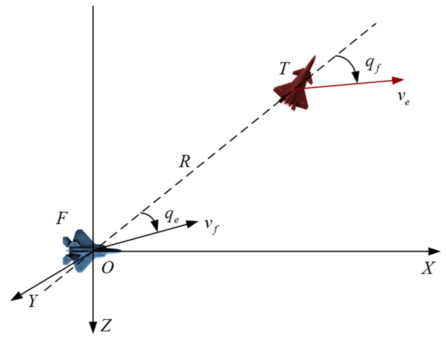
The air combat situation information mainly depends on the relative movement relationship between the air combat adversaries, as shown in Figure 1. With the center of mass position of our aircraft as the origin, the OXYZ airframe coordinate system was constructed. With the pointing direction of our aircraft head as the X axis and the Y axis as the X axis, it rotates 90 clockwise. The position is perpendicular to the X axis, the Z axis is perpendicular to the XY plane, and the direction is downward.
Assuming that the position of both sides is P f , t = [ x f , t , y f , t , z f , t ] and P e , t = [ x e , t , y e , t , z e , t ] , the relative geometric relationship between the two sides in air combat can be defined as:
R = [ x f , t x e , t , y f , t y e , t , z f , t z e , t ]
v e = P e , t P e , t 1 / Δ t
φ e , t = arc tan ( Δ z e , t / Δ x e , t ) , Δ x e , t > 0 π + arc tan ( Δ z e , t / Δ x e , t ) , Δ z e , t > 0 & Δ x e , t < 0 π arc tan ( Δ z e , t / Δ x e , t ) , Δ z e , t < 0 & Δ x e , t < 0 π / 2 , Δ z e , t > 0 & Δ x e , t = 0 π / 2 , Δ z e , t < 0 & Δ x e , t = 0
θ e , t = arc tan ( Δ y e , t / Δ x e , t + Δ z e , t )
q f = ar r cos R V f R × V f
φ f = π ar cos R V e R × V e
V f = [ v f cos γ f cos ψ f , v f cos γ f sin ψ f , v f sin γ f ]
V e = [ v e cos γ e cos ψ e , v e cos γ e sin ψ e , v e sin γ e ]
where R is the relative distance vector; V f and V e are velocity vectors of target and fighter, respectively; γ f and ψ f are the flight path angle and heading angle of the fighter, respectively; γ e and ψ e are the flight path angle and heading angle of the target, respectively; q f is the azimuth angle of the target; and φ f is the entry angle of the target. Δ x e , t = x e , t x e , t 1 , Δ y e , t = y e , t y e , t 1 , Δ z e , t = z e , t z e , t 1 , v e is the target flight speed.
There are many kinds of battlefield data that can be obtained by airborne sensors. Under the premise of considering the complexity and accuracy of the air combat situation assessment model, in this paper, the situation characteristic parameters shown in Table 1 were selected to represent the air combat situation information.
As shown in Figure 2, the air combat situation space can be divided into four categories according to the azimuth of the enemy and ourselves: advantage, disadvantage, mutual disadvantage, and mutual safe. It can be seen from Figure 2 that only the situation information at the current moment was used for evaluation, which makes the air combat situation discrete and localized, without dynamic continuity and integrity; it cannot reflect the situation between the enemy and us and cannot provide an accurate and reliable basis for tactical decision-making.
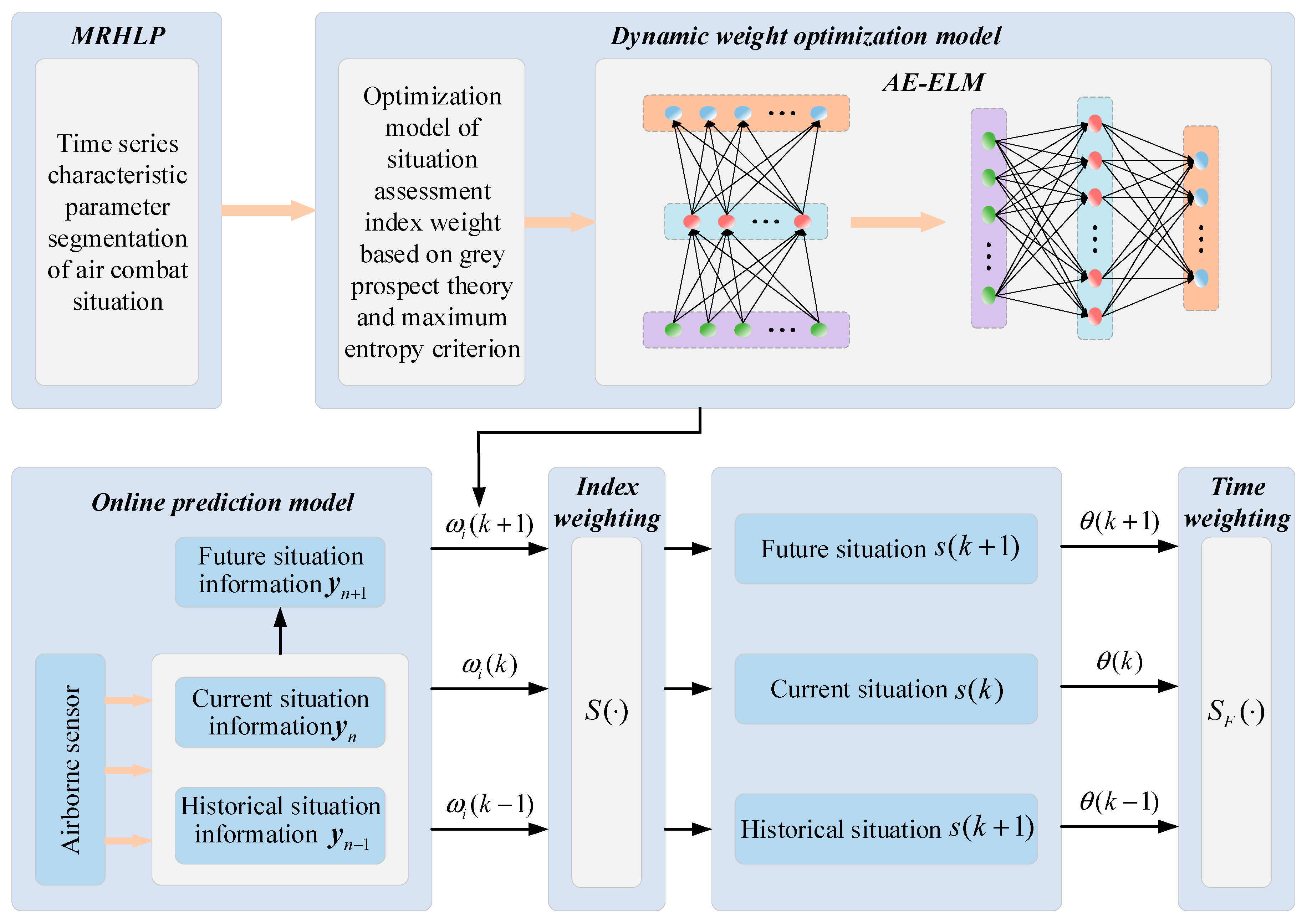
In view of the problems existing in the current air combat situation assessment model, in this paper, a dynamic air combat situation assessment model based on situation knowledge extraction and weight optimization was proposed by combining a multiple regression model of hidden logic process, a weight optimization model based on grey prospect theory, a weight mapping model based on AE-ELM, and an air combat situation characteristic parameter prediction model based on DWOSELM, as shown in Figure 3. The air combat situation assessment model presented in this paper needs to solve the following four problems.
Problem 1. Traditional situation assessment methods only use the situation information between the enemy and us at the current time to assess, which cannot reflect the timing of the air combat confrontation process, thus making the final assessment result lose tactical significance. Therefore, in this paper, the MRHLP model was used to segment the air combat situation characteristic parameters and obtain air combat situation primitives with temporal tactical significance:
s e g m e n t = MRHLP ( y 1 , y 2 , , y n ) .
Problem 2. In the process of air combat confrontation, the situation between the enemy and us is dynamically evolving, resulting in a different level of importance of each situation assessment indicator at different times or in different situation spaces. Furthermore, pilot decision preferences will have an impact on the assessment results. Therefore, the evaluation index weight should be assigned dynamically, according to the importance of the situation assessment at different situations, different moments, and different psychological decision preferences of the pilots. To solve the above problems, in this paper, combining grey theory, prospect theory, maximum entropy criterion, and an AE-ELM network, we built an adaptive solution model of evaluation index weight based on DWAE-ELM:
ω i ( k ) = DWAE - ELM ( y 1 , y 2 , , y n ) .
Problem 3. To accurately evaluate the current air combat situation between the enemy and us and provide a reliable basis for tactical and maneuver decisions, when conducting an online evaluation of an air combat situation, it is necessary to comprehensively consider its history, current situation, and future situation evolution trend, while the future situation evolution trend needs to be predicted online through the prediction model. Therefore, in this paper, combined with online learning and ELM, an online prediction model based on DWOSELM was constructed:
y n + 1 = DWOSELM ( y 1 , y 2 , , y n ) .
Problem 4. Air combat confrontation is a highly dynamic and continuous process. Only relying on the current time data for evaluation and decision-making, ignoring the hidden influence of historical information will lead to the loss of space–time relevance of the evaluation results and the rationality of the final evaluation results will be greatly reduced. Therefore, in this paper, the historical, current, and future situation information was considered comprehensively. Based on the current situation and considering the history and future, the following fusion architecture was constructed to obtain the final air combat situation:
s ( k ) = S ( y 1 , y 2 , , y n , ω i ( k ) )
s F ( k ) = S F ( s ( k 1 ) , s ( k ) , s ( k + 1 ) , θ ( k 1 ) , θ ( k ) , θ ( k + 1 ) )
where S and S F represent two nonlinear functions, which are the framework for information fusion.

3. Extraction of Air Combat Situation Primitives Based on Multiple Regression Model with a Hidden Logistic Process

In essence, the extraction of air combat situation primitives belongs to the problem of multivariate time series segmentation, that is, the time series are segmented according to different unknown hidden states and the air combat situation data with the same characteristics are divided into the same situation set, thus obtaining different air combat situation primitives. Therefore, to automatically divide the time series data of air combat situations into different time series segments, this paper extended it to multiple time series based on the hidden logic process regression model and the piecewise polynomial regression model, and an air combat situation primitive extraction algorithm based on a multiple regression model with a hidden logistic process (MRHLP) was proposed. The proposed MRHLP model is divided into two layers of regression model architecture. The regression process of observation time series is based on a piecewise polynomial regression model, while the regression process of hidden state series is based on the logistic regression model. Under the framework of HMM algorithm, automatic segmentation of air combat state time series data and accurate extraction of air combat state elements are realized.
Given a multivariate time series Y = ( y 1 , y 2 , , y n ) , where y i = ( y i ( 1 ) , y i ( 2 ) , , y i ( d ) ) T is the observed data point at time t i t = ( t 1 , t 2 , , t n ) . Assume that the observed time series is generated by a K-state hidden state series z = ( z 1 , z 2 , , z n ) , z i { 1 , 2 , , K } related to the multivariate observation time series. The MRHLP model proposed in this paper was obtained by expanding the hidden logic process regression model of univariate time series to multivariate. The hidden logic process regression model of a univariate time series can be expressed as:
y i = β z i T t i + σ z i ε i ε i ~ N ( 0 , 1 ) , i = 1 , 2 , , n
where z i { 1 , 2 , , K } is the hidden discrete state variable and governs the system state transition at time t i . β z i = ( β z i 0 , , β z i P ) T is the regression coefficient of the polynomial regression model corresponding to implicit state z i . t i = ( 1 , t i , , t i p ) T is the p + 1 dimensional covariant vector at time t i .
The model proposed in this paper can be regarded as a set of hidden logic process regression models and polynomial regression models corresponding to a one-dimensional time series, which can be specifically described as:
y i ( 1 ) = β z i ( 1 ) T t i + σ z i ( 1 ) ε i y i ( 2 ) = β z i ( 2 ) T t i + σ z i ( 2 ) ε i , y i ( d ) = β z i ( d ) T t i + σ z i ( d ) ε i
where d is the dimension of the time series. The hidden state z i governs all univariate time series components simultaneously. Therefore, multivariate time series can be jointly segmented. The model shown in Equation (12) can be converted into matrix form as follows:
y i = B z i T t i + e i e i N ( 0 , Σ z i ) , i = 1 , 2 , , n
where y i = ( y i ( 1 ) , y i ( 2 ) , , y i ( d ) ) T is the i t h observation vector; B k = [ β i ( 1 ) , β i ( 2 ) , , β i ( d ) ] is the parameter matrix of multiple regression models related to hidden state z i ; and Σ z i is the covariance matrix.
Based on the HMM model architecture, the time series pattern transition mechanism was constructed by defining the probability distribution of the hidden state variable z , which allows the time series to switch from one regression model to another. In the hidden logic regression process model, given the vector t = ( t 1 , t 2 , , t n ) , it is assumed that the variable z is independently generated by the polynomial distribution M ( 1 , π 1 ( t i ; w ) , , π K ( t i ; w ) ) , which can be expressed as:
π 1 ( t i ; w ) = P ( z i = k | t i ; w ) = exp ( w k T v i ) l = 1 K exp ( w l T v i ) ,
where π 1 ( t i ; w ) is the logistic transformation probability and is a linear function of the time-varying covariate vector v i = ( 1 , t i , t i 2 , , t i q ) ; w k = ( w k 0 , w k 1 , , w k q ) T is the q + 1 dimension coefficient vector corresponding to the time-varying covariate v i , and w = ( w 1 , w 2 , , w k ) . Due to the flexibility of the logical regression model, the RHLP model with a hidden logistic regression process is very suitable for capturing both abrupt and/or smooth changes in time series.
It can be seen from the established MRHLP model that, under the prior condition of the k t h hidden logical regression model, the observation time series y i obeys the Gaussian distribution:
p ( y i | t i ; θ ) = k = 1 K π i k ( t i ; w ) N ( y i ; β k T t i , k ) ,
where θ = ( w 1 , , w K , B 1 , , B K , 1 , , K ) is the model parameter vector to be estimated.
In this paper, the maximum likelihood method was used to estimate model parameters θ . In the classical piecewise polynomial regression model, given t = ( t 1 , t 2 , , t n ) , ε i is an independent random variable; therefore, y i is also independent. The log-likelihood function of a multivariate observation time series concerning model parameters θ can be expressed as:
L ( θ , Y , t ) = log i = 1 n p ( y i | t i ; θ ) = i = 1 n log k = 1 K π i k ( t i ; w ) N ( y i ; β k T t i , k ) .
The maximization of this log-likelihood cannot be performed in a closed form since it results in a complex nonlinear function due to the logarithm of the sum. However, in this context of the latent data model, the expectation–maximization (EM) algorithm is particularly adapted for maximizing the log-likelihood. After estimating the parameters of the MRHLP model using the EM algorithm, the time series can be segmented by calculating the label z ^ i of the polynomial corresponding to each observation x i . This can be achieved by maximizing the following polynomial logical probabilities, namely:
z ^ i = arg max 1 k K π k ( t i , w ^ ) , i = 1 , 2 , , n .
In addition, the number K of air combat situation primitives is unknown in practical applications. This paper used Bayesian information criteria to determine the number of situation primitives contained in air combat situation data:
B I C ( K , p , u ) = L ( θ ^ ) v θ log ( n ) 2
v θ = K ( d ( p + 1 + d + 1 2 ) + u + 1 ) ( u + 1 ) ,
where v θ is the number of free parameters of the model. L ( θ ^ ) is the logarithmic likelihood of the observed data obtained when the EM algorithm converges.

4. Dynamic Weight Optimization Model

Determining the weight of the evaluation index is an important part of air combat situation assessment. After studying the existing methods for determining the objective weight of indicators, the following problems were found. First, most methods determine the weight of indicators according to their differences. The core idea of these methods is to objectively assign weight to indicators by using the differences in evaluation indicators, which only reflect the importance of the differentiation between evaluation indicators and evaluation objects and do not reflect the impact of the internal relationship between evaluation objects and evaluation indicators on the importance of indicators. Second, when determining the weight of the evaluation index, the pilot is regarded as a completely rational person. However, due to the high dynamics and uncertainty of air combat confrontation, the pilot cannot maintain a completely rational psychological state in the decision-making process, which leads to the inconsistency between the weight of the index determined based on the existing methods and the actual air combat situation, thus affecting the final decision-making results. Third, the traditional index weight determination method cannot dynamically adjust its value according to the changes in various situation parameters. With the evolution of the air combat process, the influence of various situation factors on the evaluation results is not invariable. Therefore, it is necessary to constantly adjust the weight of each index to make it more reasonable to reflect the importance of each index.
To solve the above problems, a dynamic optimization model of evaluation index weight based on AE-ELM (DWAE-ELM) was constructed by combining grey correlation analysis, prospect theory, a maximum entropy criterion, and an AE-ELM network. Firstly, the concept of grey correlation depth coefficient was proposed to represent the information included in the objective weight of the index. Secondly, the prospect decision theory was introduced to characterize the decision psychological preference of pilots in the form of risk attitude coefficient and loss aversion coefficient, and then it was integrated into the evaluation index optimization model. Then, the maximum entropy optimization model was constructed to determine the weight of evaluation index under different air combat situations. Finally, based on the AE-ELM model, the dynamic mapping relationship between air combat situation characteristic parameters and index weights was constructed to dynamically update the index weights in real-time.
Definition 1.
Let  X 0 = { x 01 , x 01 , , x 0 m }  be the reference sequence and  X i = { x i 1 , x i 1 , , x i m }  be the evaluation sequence, the grey correlation coefficient of sequence  X 0 , and concerning the  j t h  index can be defined as:
γ i j = min i min j | x i j x 0 j | + ρ max i max j | x 0 j x i j | | x 0 j x i j | + ρ max i max j | x 0 j x i j | ,
 where  ρ [ 0 , 1 ]   is the resolution coefficient. On this basis, the grey relational degree can be defined as 
r i = j = 1 m ω j γ i j , i = 1 , 2 , , n .
Definition 2.
Let  γ i j +  and  γ i j  be the grey correlation coefficient between the  i t h  scheme sequence and the positive and negative ideal solutions concerning the  j t h  index. The grey correlation depth coefficient based on the positive and negative ideal solutions can be defined as: 
q i j + = γ i j + i = 1 n γ i j + · q i j = γ i j i = 1 n γ i j .
On this basis, the  q i j +  and  q i j  are called grey correlation depth coefficients based on positive and negative ideal solutions, so that grey correlation depth coefficient matrices  Q + = q i j + n × m  and  Q = q i j n × m  of the  n  evaluation schemes can be obtained.

4.1. Prospect Theory

In 1979, Kahneman et al. proposed the prospect theory through psychological test experiments [14]. Prospect theory consists of two parts, a value function and a probability weight function, and is defined as
V = i = 0 n π ( ω i ) v ( Δ x i ) ,
where V is the prospect value; p i is the weight of the i t h index; π ( p i ) is the decision weight; Δ x i is the difference concerning the reference point; v ( Δ x i ) is the decision value function, which can be expressed as:
v Δ x = σ Δ x α , Δ x 0 δ Δ x β , Δ x < 0 ,
where σ and δ are the gains sensitivity and loss avoidance coefficient of the decision-maker, respectively. If it is more sensitive to decision-making gains than decision-making losses, then σ > δ 1 . If it is more sensitive to the decision loss than the decision gain, then δ > σ 1 . α is the risk preference coefficient of decision-maker. β is the risk aversion coefficient of decision-maker. If the decision-maker is adventurous, then α , β > 1 . If the decision-maker is neutral, then α , β = 1 . If the decision-maker is conservative, then α , β < 1 .
π ( ω ) = exp γ + ( ln ω ) χ + , Δ x 0 exp γ ( ln ω ) χ , Δ x < 0 ,
where γ + , γ represents the overreaction of decision-maker. χ + and χ are the risk gain and risk loss attitude coefficients of decision-makers, respectively. If the decision-maker is adventurous, then 0 < χ + < χ < 1 . If the decision-maker is conservative, then 0 < χ < χ + < 1 . If the decision-maker is neutral, then 0 < χ + = χ < 1 .
As the risk attitude coefficient and loss avoidance coefficient reflect a psychological tendency of decision-makers, specific values cannot be derived mathematically. Therefore, relevant values can only be inferred from training data and personality characteristics. In this paper, concerning the method in [15,16], the specific process of coefficient determination is as follows:
Step1: Construct test set. That is, construct several typical decision samples for the task environment to be simulated.
Step2: Intentional testing. Let decision-makers make decisions in simulated task scenarios and record their decision results.
Step3: Set decision-maker’s decision parameters preliminarily and make decisions on scenarios in the decision sample set based on prospect theory.
Step4: Compare the decision results in Step 2 and Step 3. If the results are the same, it shows that the initial set decision parameters can well reflect the decision maker’s decision characteristics and psychological trends; otherwise, return to Step2 and continue to explore the decision parameters until the decision results in Step2 and Step3 are consistent.

4.2. Maximum Entropy Objective Weight Optimization Model of Situation Assessment Index Based on Grey Prospect Theory

Grey correlation analysis not only determines the degree of correlation among the sequences but also reflects the internal correlation of the attributes of each evaluation index in the behavior sequence, and ignores the internal correlation among evaluation indicators. To reflect the importance of evaluation indicators more objectively and comprehensively, the concept of grey correlation depth coefficient is introduced to quantify the internal correlation among the attributes of evaluation indicators when determining the weight of indicators, so as to reflect their importance.
In addition, in the air combat decision-making process, to better reflect the characteristic that pilots cannot always maintain complete rationality in the fierce air combat environment, in this paper, prospect theory was introduced into the optimization model of determining the weight of air combat situation indicators to describe the uncertainty of pilots’ decision-making preferences. Prospect theory introduces people’s decision-making psychological preferences into the decision-making process, and quantifies this psychological preference in the form of risk attitude coefficient, loss avoidance coefficient, etc. For different pilots, the parameters are different, and these coefficients reflect the attitude of pilots to combat decision-making risks. At the same time, the psychological tendency of pilots will also change during the whole air combat process.
When determining the weight of air combat situation assessment indicators, the weight of indicators is determined by combining the decision preference of pilots in different operational scenarios and the amount of information contained in each assessment indicator data. According to the maximum entropy criterion, based on the known part of the information, it is considered that the weight obtained by maximizing the entropy value of the weight and meeting the constraint conditions is most likely. Therefore, based on the maximum entropy criterion, the objective weight optimization model of a maximum entropy situation assessment index based on gray prospect theory was constructed. The specific steps are as follows:
Step1: Standardize the evaluation index values to obtain the evaluation index matrix F = ( x i j ) n × m of all schemes.
Step2: Determine a positive ideal solution and a negative ideal solution. Let x + be the positive ideal solution and x the negative ideal solution, which can be expressed as:
x + = max i   x i j | x i j X + , min i   x i j | x i j X = x 1 + , x 2 + , , x m + x = min i   x i j | x i j X + , max i   x i j | x i j X , = x 1 , x 2 , , x m
where X + is a benefit index and X is a cost index.
Step3: Construct the positive and negative grey correlation depth coefficient matrix γ + = γ i j + n × m and γ = γ i j n × m , respectively.
Step4: Based on the grey correlation depth coefficient matrix of positive and negative ideal solutions and the concept of value function in prospect theory, the positive and negative prospect value matrix is constructed.
v i j + ( γ i j ) = σ ( γ i j ) α
v i j ( γ i j + ) = δ ( γ i j + ) β .
Step5: Calculate the gray prospect coefficient of each evaluation index
ζ i j = | v i j ( γ i j + ) | | v i j ( γ i j + ) | + | v i j ( γ i j ) | .
Step6: Determine the range of the weight of each evaluation index.
The grey prospect coefficient obtained by combining the grey correlation depth coefficient and the prospect theory objectively reflects the correlation between different indicators and the regularity between different indicators and schemes, as well as the impact of the decision-maker risk preference psychology on the indicator weight.
According to the above idea of objective weight determination, the index weight is limited between the maximum and minimum values of the corresponding normalized gray foreground coefficient, and the dynamic variation range of the weight is constructed as follows:
ω j [ min i ( η i j ) , max i ( η i j ) ] i = 1 , 2 n ; j = 1 , 2 , m .
Step7: Determine the constraint of the index weight variance fluctuation range.
The fluctuation range of the index weight is also determined by the gray prospect coefficient. The constraints on the variance of index weight can be introduced as follows:
1 m j = 1 m ( ω j 1 m ) 2 ( min ( D i ) , max ( D i ) )
D i = 1 n i = 1 n ( η i j 1 n ) 2 .
Step8: Establish the maximum entropy optimization model of the evaluation index weight.
Using the weight change and fluctuation constraints in Step6 and Step7, an objective weight maximum entropy optimization model based on gray prospect coefficient was constructed as follows:
max F = j = 1 m ω j ln ω j s . t .   j = 1 m ω j = 1 , ω j [ min i ( η i j ) , max i ( η i j ) ] 1 m j = 1 m ( ω j 1 m ) 2 ( min ( D i ) , max ( D i ) )
where ω j represents the weight of the j t h index. D i is the variance of gray prospect coefficient of the i t h index, reflecting the change range of the indicator weight.

4.3. AE-ELM-Based Air Combat Situation Assessment Index Weight Mapping Model

In the air combat situation assessment index system, with the continuous evolution of the confrontation process, the impact of each situation index on the assessment results is also dynamic. In addition, the correlation and coupling between air combat situation characteristic parameters are not conducive to describing air combat situations. Therefore, in this paper, the autoencoder and extreme learning machine were used to construct the mapping relationship between air combat situation feature parameters and evaluation index weight, so as to provide the dynamic situation index weight reflecting the combat process in real-time.
(1)
Autoencoder
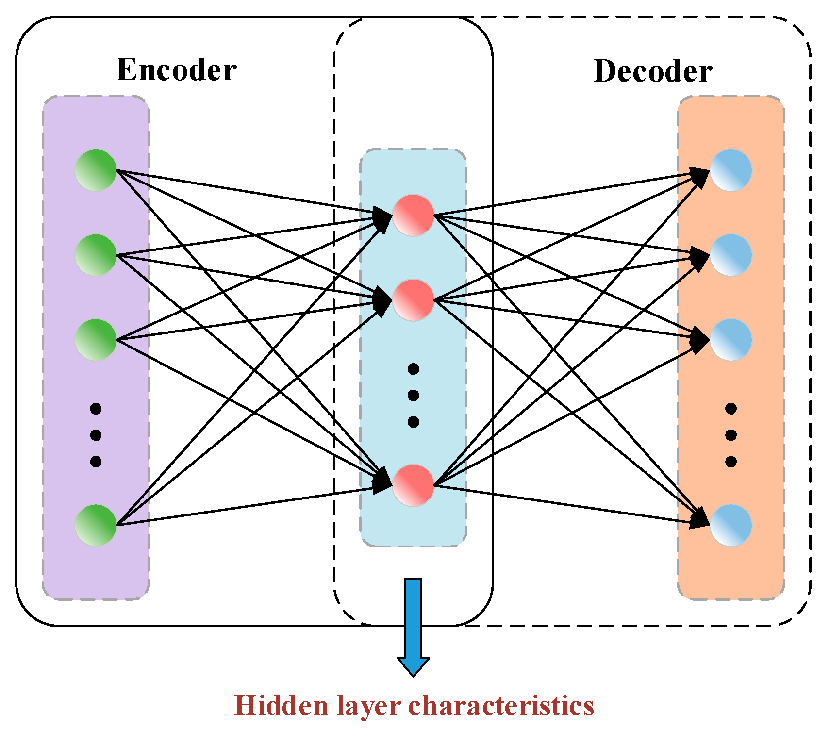
Autoencoder (AE) is a typical unsupervised algorithm, usually used for feature extraction, data compression, data visualization, etc. AE has a symmetrical three-layer network structure, mainly including an encoder and decoder. The specific structure is shown in Figure 4.
Based on the autoencoder structure in Figure 4, the encoding and decoding process of the autoencoder can be described as:
h = σ e ( W e x + b e ) R v
x ^ = σ d ( W d h + b d ) R u ,
where x is the input vector. h is the output of the encoder. x ^ is the output of the decoder. W e , b e are the weight and bias of the encoder, respectively. W d , b d are the weight and bias of the decoder, respectively. σ e , σ d are the nonlinear activation functions of the encoder and the decoder, respectively. Different optimization objective functions can be constructed according to different loss criteria and the optimization objective functions can be constructed based on the energy loss criteria as follows:
min θ J ( θ ) = 1 N n = 1 N x ^ ( n ) x ( n ) 2 2 + λ R ( θ ) ,
where θ is the parameter set to be optimized in autoencoder and R ( θ ) is the optimization regular term, which can be defined as:
θ = [ W a , b a ; W s , b s ] R ( θ ) = W a F 2 + W s F 2 .
(2)
Extreme learning machine
Extreme learning machine was put forward in 2004. It is an effective learning algorithm for feedforward neural networks with a single hidden layer. Compared with the traditional feedforward neural network with a single hidden layer, this algorithm can effectively overcome the shortcomings of the traditional neural network, which easily fall into the local extreme value due to the training with the gradient descent method and has the advantages of fast learning speed and strong generalization ability.
Given N training samples ( x j , t j ) , where x j = [ x j 1 , x j 2 , , x j n ] T R n , t j R . Assuming that the number of nodes in the hidden layer is L and the activation function is g ( x ) , the output of ELM can be expressed as:
O j = i = 1 L β i g ( w i x j + b i ) , j = 1 , 2 , , N ,
where W i and β i are the input weight and output weight of the i t h hidden layer node, respectively; b i is the bias of the i t h node of the hidden layer.
To make the error between the predicted result of the network and the true value close to zero, that is, j = 1 N O j t j = 0 , it is necessary to find a group of appropriate network parameters to make:
i = 1 L β i g ( w i x j + b i ) = t j , j = 1 , 2 , , N .
The above equation can be transformed into a matrix expression:
H β = T ,
where H is the output matrix of the hidden layer. The least square method is used to solve Equation (43) to obtain the weight matrix β ^ of the network output:
H β ^ T = H H T T = min β H β T .
When the calculation error approaches zero, it can be obtained that
β ^ = H T ,
where H is the Moore Penrose of H .
(3)
Dynamic mapping model of situation assessment index weight based on AE-ELM
Based on the optimization model of situation assessment index weight proposed in Section 4.2, combined with AE and ELM, a mapping model of situation assessment index weight based on AE-ELM was constructed. The main idea is as follows: first, under different situations, the corresponding index weights are obtained by using the maximum entropy weight optimization model based on gray prospect theory. Then, the AE is used to compress and reduce the dimension of air combat situation characteristic parameters to eliminate the correlation between parameters. Finally, the mapping relationship between the processed situation characteristic parameters and the index weights is established by using the ELM. The specific steps are as follows:
Step1: Under different air combat situations, establish an air combat situation index weight optimization model based on the gray prospect theory to obtain the index weights corresponding to different situations.
Step2: Initialize the AE-ELM parameter. Randomly initialize the weights and bias of AE and ELM, respectively.
Step3: The parameters of the AE are obtained by unsupervised training. The gradient descent method is used to train the AE to obtain the optimal weight and bias.
Step4: The parameters of the ELM are obtained by supervised training. The situation index weight obtained by Step1 and the trained AE model are used to build the training sample data set of ELM. On this basis, by solving the generalized Moore–Penrose inverse of the matrix H , the output weight of ELM is obtained, and the mapping relationship between the air combat situation parameters and the evaluation index weight is output.

4.4. Timing Weight Analytical Model Based on Normal Cumulative Distribution Method

Air combat is a highly dynamic and continuous confrontation process. Only using the current moment information will ignore the impact of historical information on the situation evaluation results, so it is impossible to make an objective and comprehensive analysis of the continuous air combat situation, which leads to greatly reducing the rationality of the final evaluation results. Therefore, it is necessary to deeply analyze the association between the air combat situation at multiple consecutive times and the current air combat situation assessment. In this paper, a time series weight calculation model based on normal cumulative distribution was established and the time series weight was analyzed using the algorithm of the normal cumulative distribution function [17]. The normal cumulative distribution function is introduced and defined as follows:
F ( t k ; μ p , σ p ) = 1 2 π σ p k exp ( ( t μ P ) 2 σ p ) d t , k = 1 , 2 , 3 , , p , t > 0 .
An error function is used to represent the cumulative distribution function of the normal distribution:
ϕ ( z ) = 1 2 1 + e r f ( z μ p 2 σ p ) ,
where μ p is the mean value of set 1 , 2 , 3 , , p ; σ p ( σ p > 0 ) is the standard deviation and satisfies the following relations:
μ p = 1 p p ( 1 + p ) 2 = 1 + p 2
σ p = 1 p k = 1 p ( k μ p ) 2 .
The timing weight based on the cumulative distribution function obeying normal distribution can be obtained:
θ ( t k ) = F ( t k ; μ p , σ p ) k = 1 p F ( t k ; μ p , σ p ) = k exp ( ( t μ p ) 2 σ p ) d t k = 1 p k exp ( ( t μ p ) 2 σ p ) d t ,
where θ ( t k ) is the weight at time t k and p is the number of consecutive moments.

5. A Situation Prediction Model Based on a Dynamic Weighted Online Extreme Learning Machine

5.1. OS-ELM

The training process of ELM is based on the fixed training dataset X . Therefore, the prediction model based on ELM corresponds to the training samples. When new training samples with different distributions from the fixed training dataset X are input into the prediction model, the model needs to be retrained to improve the prediction performance of the model. However, the training process of ELM contains complex matrix operations. Each additional matrix operation of the new training data will greatly increase the complexity of the model, thus reducing the real-time performance of the online prediction of ELM. To solve the contradiction between the real-time calculation output weight of ELM and the real-time prediction, an OS-ELM algorithm that can calculate the output weight of ELM in real time through recursion was constructed.
Given the training sample data set D = { ( x j , t j ) } 1 N , t j is the expected output of sample x j , T = [ t 1 , t 2 , , t N ] . The node equations in the hidden layer of the ELM can be reconstructed into the following matrix expression:
H β = Τ
H ( ω 1 , ω 2 , , ω N ˜ , b 1 , b 2 , , b N ˜ , x 1 , x 2 , , x N ) = g ( ω 1 x 1 + b 1 ) g ( ω 2 x 1 + b 2 ) g ( ω N ˜ x 1 + b N ˜ ) g ( ω 1 x 2 + b 1 ) g ( ω 2 x 2 + b 2 ) g ( ω N ˜ x 2 + b N ˜ ) g ( ω 1 x N + b 1 ) g ( ω 2 x N + b 1 ) g ( ω N ˜ x N + b N ˜ ) N × N ˜
β = [ β 1 , β 2 , , β N ˜ ] N ˜ × m T ,
where H is the hidden layer output matrix of the ELM.
Based on the principle of structural risk minimization in statistical theory, the empirical risk and structural risk are minimized simultaneously in the process of algorithm learning, and the minimum squares method is used to solve the following optimization problems:
min F = C 2 H β T 2 2 + 1 2 β 2 2 ,
where C is the regularization parameter. The output weight of ELM can be obtained by derivation of Equation (54) as follows:
β = ( H T H + I / C ) 1 H T T .
According to the output weight β of ELM, the predicted value of the sample can be obtained:
f m ( x i ) = l = 1 L β l m g ( a l , b l , x i ) .
The OSELM model is a combination of ELM and online learning. Its network topology is the same as that of ELM. The OSELM model can be learned sample by sample or in batches to update the output weight of the network online. The training of the OSELM model includes two stages: an initialization stage and an online learning stage. Given training sample data block set D 0 , D 1 , , D K , D k = { ( x k i , t k i ) } 1 N k , N k is the number of samples in the k t h sample block.
(1)
Initialization stage
The input weight matrix a R × L and the hidden layer bias vector b L of the model are randomly initialized. According to the initial sample data block D 0 and the output weight expression in Equation (55), the initial network output weight can be obtained:
β 0 = ( H 0 T H 0 + I / C ) 1 H 0 T T 0 = L 0 H 0 T T 0 ,
where K 0 = H 0 T H 0 + I / C , T 0 = [ t 1 , t 2 , , t N 0 ] T , L 0 = K 0 1 .
(2)
Online learning stage
When the k t h sample data block D k is obtained, the model output weight β k is updated in real-time:
β k = I C + H k 1 h k T H k 1 h k 1 H k 1 h k T T k 1 t k = K k 1 H k 1 h k T T k 1 t k = K k 1 ( H k 1 T T k 1 + h k T t k ) .
Let L k = K k 1 , we can get:
L k = I C + H k 1 h k T H k 1 h k 1 = L k 1 L k 1 H k ( I + H k L k 1 H k T ) 1 H k L k 1 .
Substituting Equation (59) into Equation (58) can we get:
β k = β k 1 + L k 1 H k T ( T k H k β k 1 ) .
For now, the real-time update expression of the model is obtained:
L k = L k 1 L k 1 H k ( I + H k L k 1 H k T ) 1 H k L k 1 β k = β k 1 + L k 1 H k T ( T k H k β k 1 ) .

5.2. DWOSELM

Based on the approximation theory of ELM, OSELM transformed the training problem of single hidden layer feedforward neural networks into a problem of solving linear equations, and the recursive least squares (RLS) method was used to recursively calculate the output weights to achieve online updating of the algorithm. Compared with other common online learning algorithms, OSELM not only has better generalization performance but also has obvious advantages in learning speed, which can well solve the problem of time series prediction. However, due to the natural sensitivity of RLS to noisy data, the generalization performance of the OSELM algorithm based on RLS will be seriously degraded in noisy or outlier environments. Compared with other common online learning algorithms, OSELM not only has better generalization performance but also has obvious advantages in learning speed, which can solve the time series prediction problem well. However, the natural sensitivity of RLS methods to noisy data also severely reduces the generalization performance of RLS-based OSELM algorithms in noisy or outlier environments.
To enhance the robustness of OSELM in outlier environment, a dynamic weight online extreme learning machine (DWOSELM) prediction model was proposed in this paper. DWOSELM model inherits the basic idea of OSELM sequential learning and carries out inverse weighting calculation based on the prior error of samples in the online learning process, so as to reduce the influence of outliers on the learning model. The sample dynamic weighting matrix is introduced:
W = diag ( w 1 , w 2 , , w n ) ,
where n is the number of samples and w i is the weight of the i t h sample, which can be expressed as:
w k = min ( 1 , 1 h k e k )
where e k = y k h k β k , is the prior error of the current sample.
After introducing the sample dynamic weighting matrix, the output weight of the DWOSELM model at the initial stage can be expressed as follows:
β 0 = K 0 1 H 0 T W 0 T 0
K 0 = H 0 T W 0 H 0 + I / C ,
where W 0 = d i a g ( ω 01 , ω 02 , , ω 0 N 0 ) is the weight matrix of the initial sample data block. The model parameter β k in the online learning stage can be expressed as:
β k = I C + H k 1 h k T W k 1 W k H k 1 h k 1 × H k 1 h k T W k 1 W k T k 1 t k ,
where W k is the weight matrix of the k t h sample data block. According to Equations (66) and (58), K k can be expressed as:
K k = I C + H k 1 h k T W k 1 W k H k 1 h k = I C + H k 1 T W k 1 H k 1 + h k T W k H k = K k 1 + h k T W k H k .
The second half of Equation (66) can be expressed as:
H k 1 h k T W k 1 W k T k 1 t k = H k 1 T W k 1 T k 1 + h k T W k t k = K k 1 K k 1 1 H k 1 T W k 1 T k 1 + h k T W k t k = K k 1 β k 1 + h k T W k t k = ( K k h k T W k h k ) β k 1 + h k T W k t k = K k β k 1 h k T W k h k β k 1 + h k T W k t k .
By substituting Equations (67) and (68) into Equation (66), the real-time updating formula of model output weight can be obtained:
β k = K k 1 H k 1 h k T W k 1 W k H k 1 h k = K k 1 ( K k β k 1 h k T W k h k β k 1 + h k T W k t k ) = β k 1 + K k 1 h k T W k ( t k h k T β k 1 ) .
Let, L k = K k 1 we can get:
L k = L k 1 L k 1 ( W k 1 + H k L k 1 H k T ) 1 H k L k 1
β k = β k 1 + L k h k T W k ( t k T h k β k 1 ) .
The DWOSELM model is more robust and practical than the similar algorithms, and it can improve the operation speed of the algorithm under the premise of ensuring the calculation accuracy.

6. Construction of Air Combat Situation Assessment Model

6.1. Air Combat Situation Evaluation Index System

A large number of air combat simulations show that a favorable air combat situation is the premise for the fighter to preempt. In this paper, four evaluation indicators, namely angle, speed, height, and distance, were selected to build an air combat situation assessment model.
(1)
Angle advantage
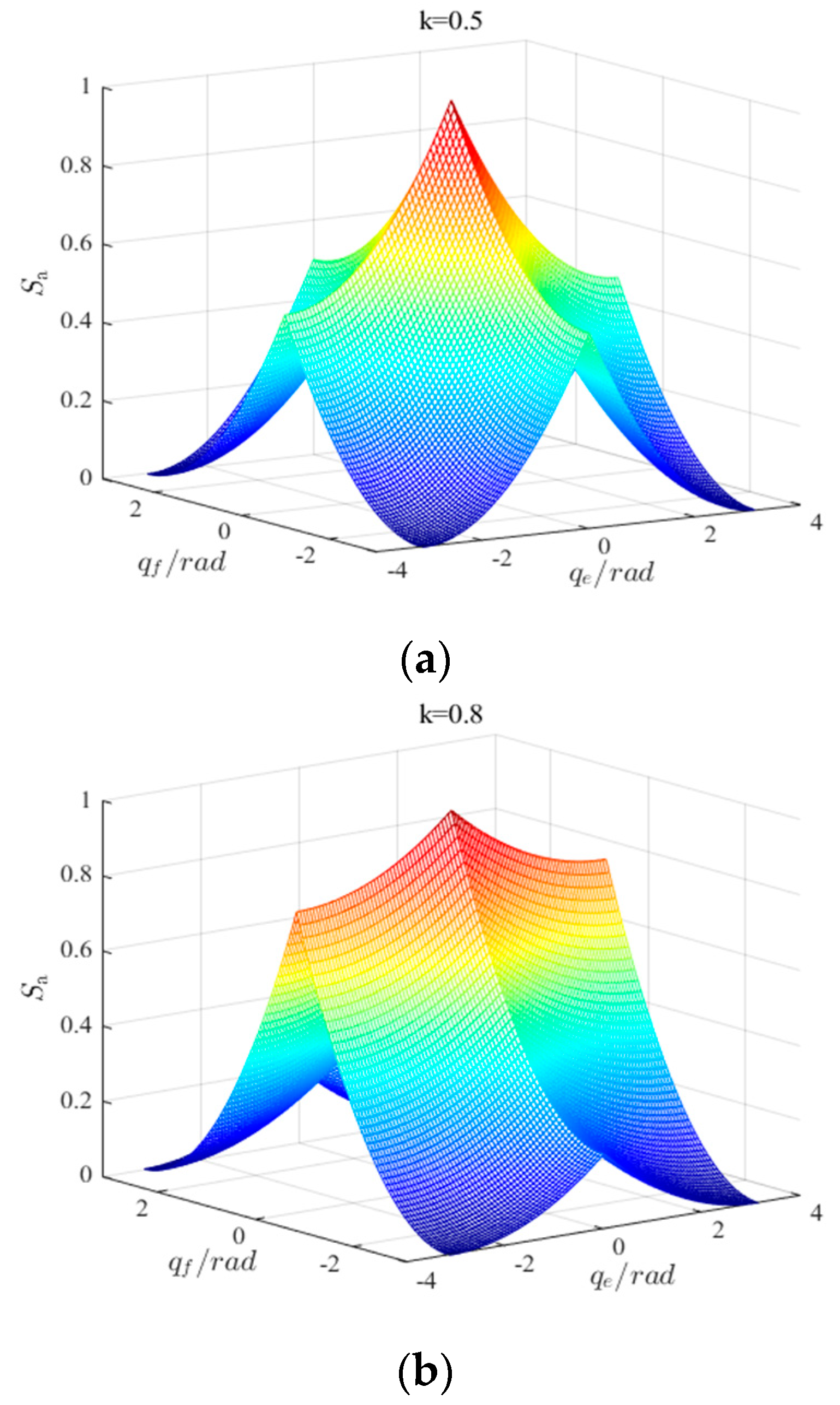
According to the geometric relationship of air combat situation between the enemy and us shown in Figure 1, the smaller the azimuth angle q e of the enemy is, the more opportunities for us to attack the target. Similarly, the smaller our azimuth q f is, the lower the probability of us being attacked by the target. Therefore, in this paper, the air combat situation angle advantage function is defined as:
S a = ( k ( π q e ) 2 + ( 1 k ) ( π q f ) 2 ) / π .
Different pilots may evaluate specific situations differently based on their own experience and intuition. Therefore, the parameters in Equation (72) are used to characterize the decision-making tendency of pilots under different conditions. The relationship between azimuthal angle of enemy, azimuthal angle of fighter, and angle advantage function are shown in Figure 5.
(2)
Distance advantage
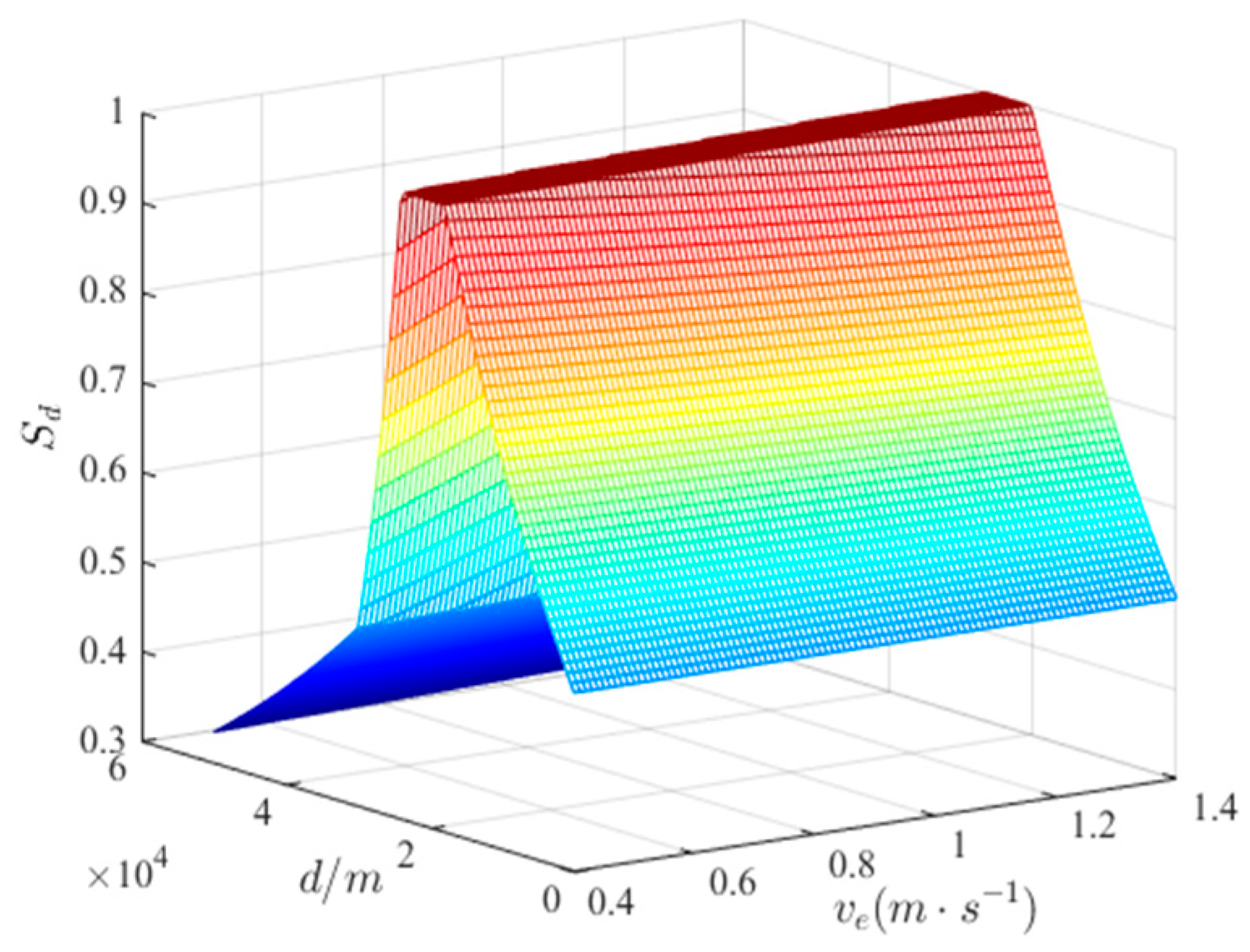
The influence of distance on the advantage function is mainly reflected in the attack zone boundary, airborne radar detection probability, and missile kill probability. Based on the above analysis, the distance advantage function is defined as
S d = 0 , d D r max 1 5 e d D M max D r max D M max , D M max d < D r max 2 d D M K max D M max D M K max , D M K max d < D M max 1 , D M K min d < D M K max 2 d D M K min D M min D M K min , D M min d < D M K min 1 5 e d D M min D M min D r min , D r min d < D M min 0 , d < D r min ,
where D r max is the maximum detection range of airborne radar. D M max and D M min are the far boundary and near boundary of the attack area, respectively. D M K max and D M K min are the far boundary and the near boundary of the non-escape zone. D r min is the collision avoidance safety distance of the enemy. The relationship between the speed of enemy, the distance between us and the enemy, and the distance superiority function are shown in Figure 6.
(3) Speed advantage
In the actual air combat, the party with the speed advantage has more air combat advantage, but too fast a speed will lead to poor mobility and other deficiencies. Therefore, we used for reference the idea of “variable speed to the enemy”, using the desired speed to construct the speed advantage function.
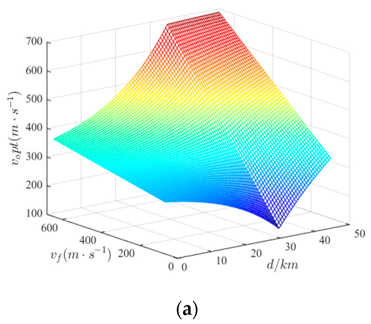
v o P t = v f + ( v max v f ) ( 1 e d D K max D K max ) , d D K max v f + ( v min v f ) ( 1 e 2 ( d D K max ) D K max ) , D K min < d < D K max
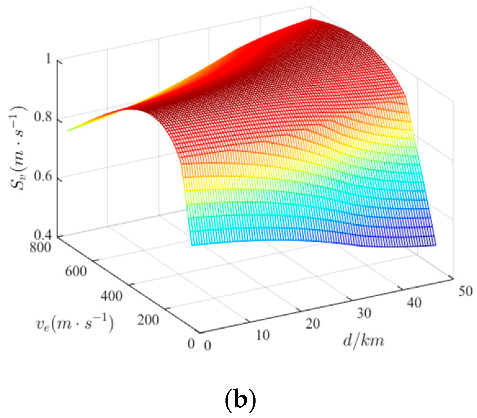
S v = v f v e e 2 v e v o P t v o P t 2 v o P t 1 2 ,
where v o P t is the expected speed. v max and v min are the maximum and minimum flight speeds of the enemy, respectively. d is the relative distance between enemy and us. The relationship between expected speed and distance and the carrier speed is shown in Figure 7a, and the relationship between speed advantage and expected speed, and distance, is shown in Figure 7b.
(4)
Height Advantage
Drawing on the construction method of speed advantage function, the expected height is introduced to construct the height advantage function:
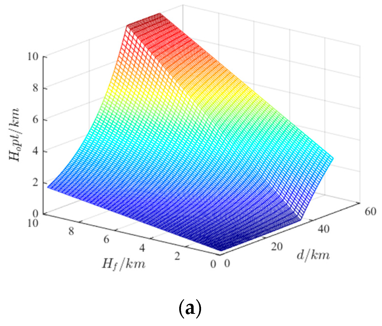
H o P t = H f + ( H max H f ) ( 1 e d D K max D K max ) , d D K max H f + ( H min H f ) ( 1 e 2 ( d D K max ) D K max ) , D K min < d < D K max
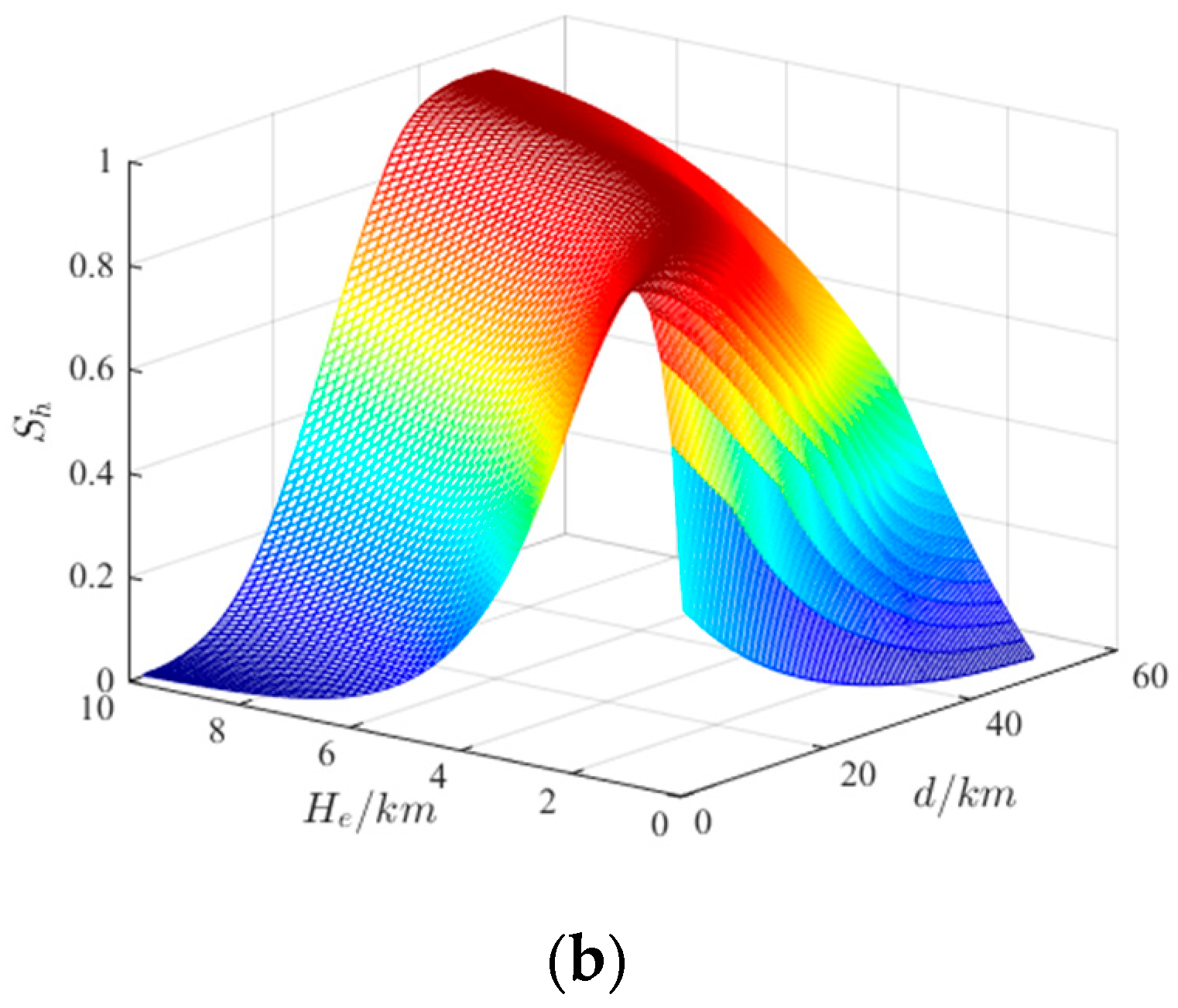
S h = ( H f H o P t e 2 H e H o P t H o P t 2 H o P t ) 1 2 , H f [ H min , H max ] 0 , H f [ H min , H max ] ,
where H min is the safe flight height of the enemy. H max is the maximum flight height of the fighter. H f is the flight height when the fighter launches missiles. H o P t is the expected flight height of the fighter. H e is the flight height of the enemy. The relationship between expected height and carrier height, and distance, is shown in Figure 8a, and the relationship between height advantage and expected height, and distance, is shown in Figure 8b.

6.2. The Process of Air Combat Situation Assessment Model

Aiming at the shortcomings of the current air combat situation assessment model, a dynamic air combat situation assessment model based on situation knowledge extraction and weight optimization was proposed by combining the multiple regression model with a hidden logistic process, the weight optimization model based on gray prospect theory, the weight mapping model based on AE-ELM, and the air combat situation characteristic parameter prediction model based on DWOSELM. The specific implementation steps of the evaluation model are as follows.
Step1: Extract a large number of medium-range confrontation trajectory data from the air combat simulation training system, calculate and extract the characteristic parameters of the air combat situation.
Step2: Use the MRHLP model to segment the time series data of air combat situation characteristic parameters and extract air combat situation primitives.
Step3: Use the maximum entropy objective weight optimization model of situation assessment indicators based on gray prospect theory to calculate the objective weight of air combat situation indicators under different situations.
Step4: Use the AE-ELM model to build dynamic mapping relationship between situation characteristic parameters and indicator weights.
Step5: Use the DWOSELM model to predict the target maneuver trajectory, estimate the future situation information between the enemy and us, and calculate the future air combat situation.
Step6: The time weight calculation model based on normal cumulative distribution is used to determine the importance of the situation at each time. The situation information at multiple times in the air combat process is fused to obtain the comprehensive air combat situation assessment results at the current time.

7. Simulation Analysis

7.1. Performance Verification of Multivariate Time Series Segmentation Based on MRHLP

To verify the effectiveness and robustness of the MRHLP algorithm in multivariate time series segmentation point detection, this algorithm was compared with six kinds of algorithms in the literature.
(1)
MHMMR [18] (Multiple hidden Markov model): An unsupervised multivariate time series segmentation model based on hidden Markov model regression.
(2)
MPWR [19] (multiple polynomial piecewise regression model): an optimal segmentation method for multivariate time series based on polynomial piecewise regression model.
(3)
ACA [20] (Aligned cluster analysis): The problem of time series segmentation is transformed into the problem of time series clustering, and a method of alignment clustering analysis based on dynamic time alignment kernel and dynamic programming was proposed.
(4)
HACA [21] (Hierarchical aligned cluster analysis): An unsupervised bottom-up hierarchical aligned cluster analysis method was proposed by combining the standard vector space clustering method, dynamic time alignment kernel, and dynamic programming.
(5)
A segmentation method based on data point clustering: GMM [22], SC, FCM [23], and k-means clustering algorithms were used to directly cluster multivariate time series data, and discrete classification labels were used to segment time series data.
(6)
KPCA-GG [24]: A multivariate time series segmentation algorithm based on kernel principal component analysis and Gath Geva fuzzy clustering.
In essence, the problem of multivariate time series segmentation is to divide a long time series into segments of multivariate time series with different lengths and patterns. It can be regarded as a clustering problem of multivariate time series or a classification problem. In this paper, we regarded it as a classification problem and used accuracy, precision, recall, F1 score, specificity, and Gmean to evaluate the performance of each segmentation algorithm.
(1)
Accuracy
A c c u r a c y = T P + T N T P + T N + F P + F N
(2)
Precision
P r e c i s i o n = T P T P + F P
(3)
Recall
R e c a l l = T P T P + F N
(4)
F1-score
F 1 s c o r e = 2 P r e c i s i o n R e c a l l P r e c i s i o n + R e c a l l
(4)
Specificity
S p e c i f i c i t y = T N T N + F P
(5)
Gmean
G m e a n = R e c a l l × S P e c i f i c i t y
The meaning of the above formula is shown in Table 2.

7.1.1. Segmentation Performance Verification of Algorithm Based on Simulation Data

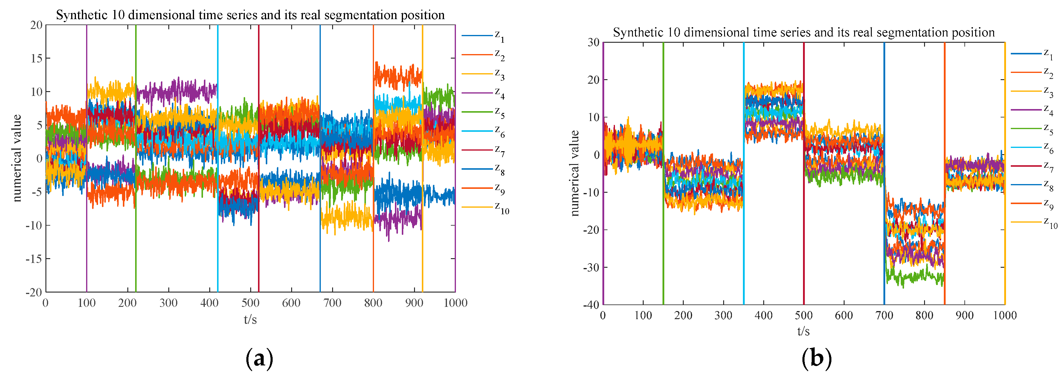
The advantage of using synthetic datasets to verify the segmentation performance of the algorithm is that the correct segmentation is known, which is convenient for evaluating its performance. In this paper, the first-order vector autoregression model [25] was used to generate two sets of 10-dimensional time series data sets. The number of data points is 1000, including eight and six modes, respectively. The specific model expressions are as follows:
Z ( t ) = ϑ 1 + ϑ 2 Z ( t 1 ) + u ( t )
where Z ( t ) = [ z 1 ( t ) , z 2 ( t ) , , z 10 ( t ) ] , t = 1 , 2 , , 1000 is a multivariate Gaussian with mean 0 and variance Σ = I .
Two multivariate time series were generated based on Equation (88), and the generated multivariate time series is shown in Figure 9. The details are as follows:
(1)
Generate a 10-dimensional time series containing eight sub-segments, and the real segmentation positions are 100, 220, 420, 520, 670, 800, 920, and 1000.
(2)
Generate a 10-dimensional time series containing six sub-segments, and the real segmentation positions are 150, 350, 500, 700, 850, and 1000.
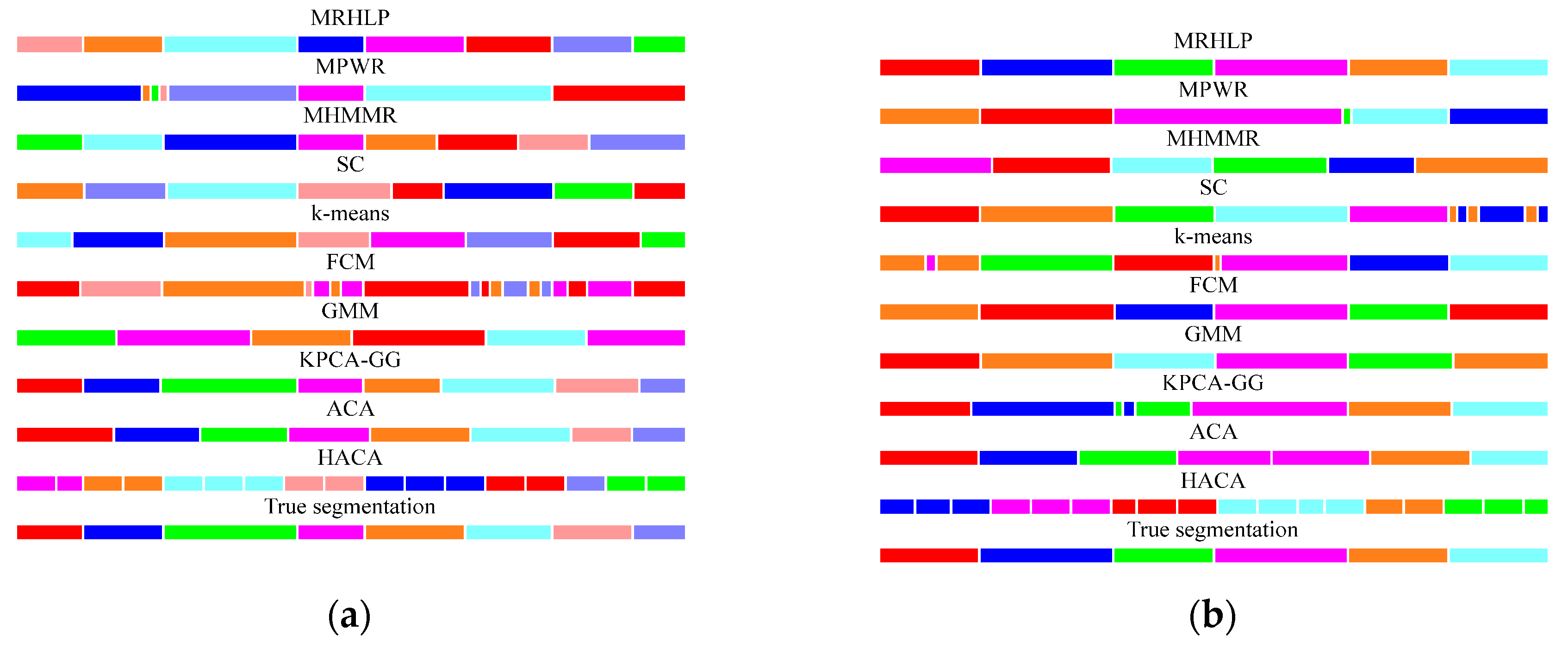
Figure 10 presents the segmentation results for two sets of synthetic data under different algorithms. As can be seen from Figure 10, on the two sets of synthetic multivariate time series, the proposed MRHLP algorithm can achieve more accurate segmentation results, which are relatively close to the real segmentation position, indicating the effectiveness of the MRHLP algorithm in handling multivariate time series segmentation problems.
To better verify the performance of the algorithm, the MRHLP multivariate time series segmentation algorithm proposed in this paper was compared with KPCA-GG, GMM, SC, k-means, FCM, MHMMR, MPWR, ACA, and HACA in terms of average Precision, Recall, Accuracy, Specificity, F1-score, and Gmean under the two synthetic datasets. The performance comparison results are shown in Table 3 and Table 4. It can be seen that, on the synthetic multivariate time series 1, the MRHLP algorithm can segment it very accurately, while the segmentation results obtained by other algorithms have certain errors. On the synthetic multivariate time series 2, the segmentation performance indicators of the MRHLP algorithm are close to 1, and the performances of the other algorithms are biased. In conclusion, the algorithm proposed in this paper has the best performance, can relatively accurately segment the multivariate time series, and achieve a segmentation result closer to the real segmentation situation.

7.1.2. Segmentation Performance Verification of Algorithm Based on Air Combat Situation Data

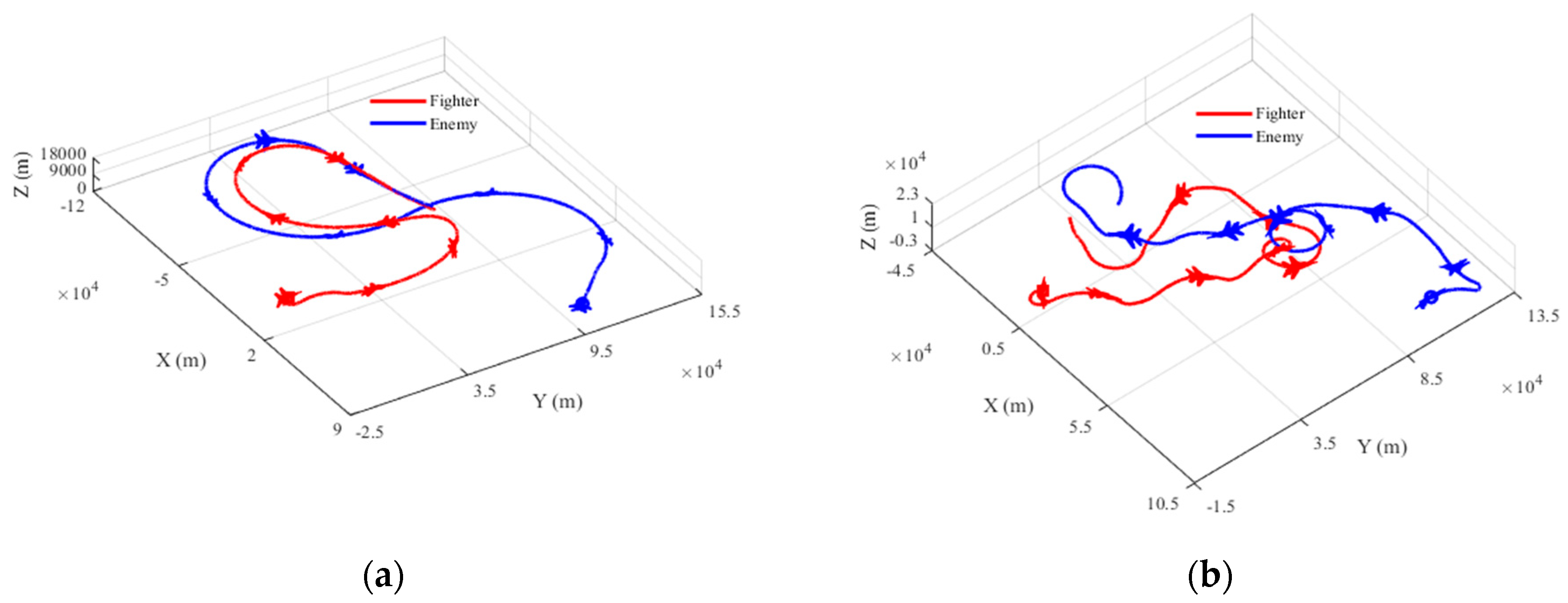
To verify the feasibility and effectiveness of the MRHLP multivariate time series segmentation algorithm in solving the problem of extracting medium-distance air combat situation primitives, two groups of air combat trajectory data as shown in Figure 11 were selected from the air combat training system to test the performance of the algorithm, and the algorithm was compared with six algorithms in the literature.
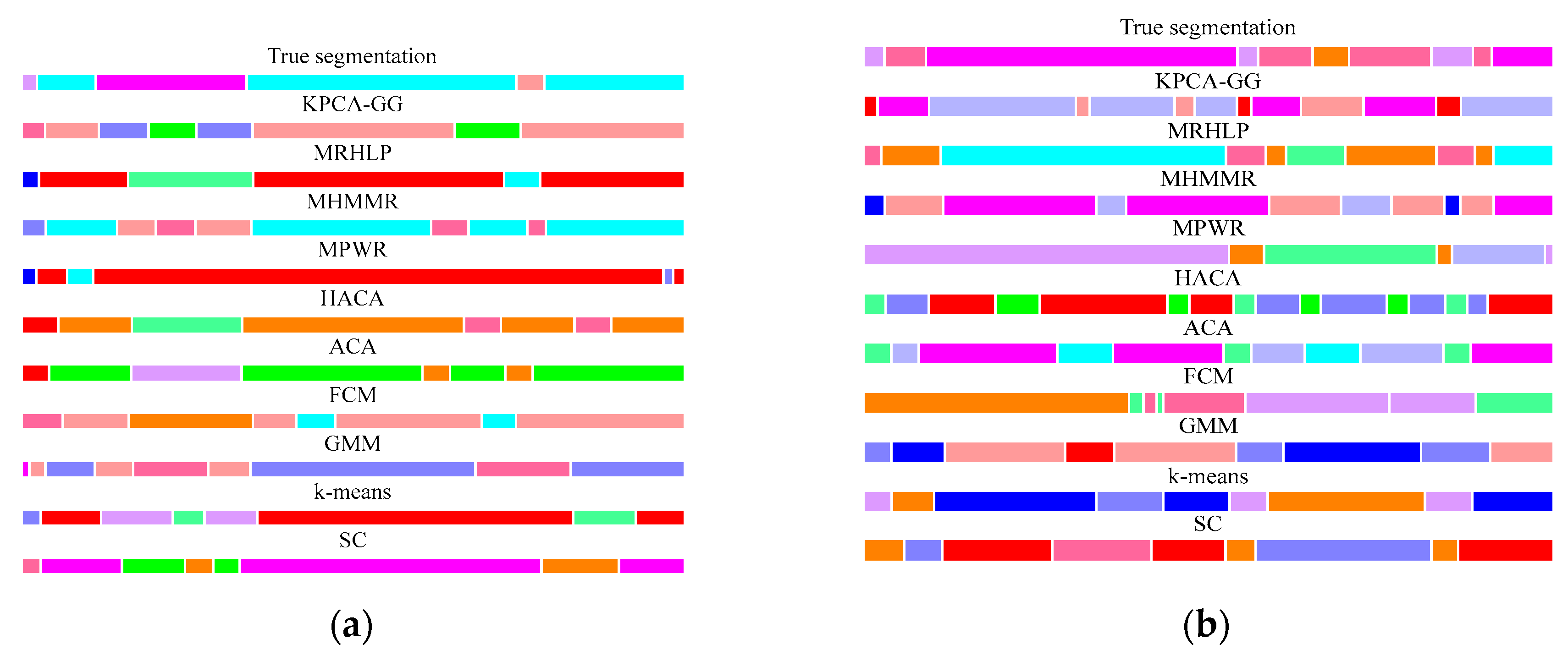
Figure 12 shows the segmentation results of two groups of real air combat trajectory data under different algorithms. It can be seen that the MRHLP algorithm proposed in this paper can obtain more accurate segmentation results on two groups of real air combat trajectory data, which is closer to the real segmentation position, indicating that the MRHLP algorithm can effectively deal with the problem of time series segmentation of air combat situation characteristic parameters, and accurately divide the air combat confrontation process into different air combat situation primitives.
To better verify the performance of the algorithm, the MRHLP multivariate time series segmentation algorithm proposed in this paper was compared with KPCA-GG, GMM, SC, k-means, FCM, MHMMR, MPWR, ACA, and HACA in terms of average Precision, Recall, Accuracy, Specificity, F1 score and Gmean under two groups of real air combat trajectory data. The performance comparison results are shown in Table 5 and Table 6.
On the two groups of real air combat trajectory data, the MRHLP algorithm performs better than the other nine algorithms in multivariate time series segmentation. It can relatively accurately segment the time series of air combat situation characteristic parameters and can obtain trajectory fragments reflecting different air combat situations, providing a reliable data basis for the optimization of evaluation weights.

7.2. Verification of Air Combat Situation Prediction Model Based on DWOSELM

To verify the effectiveness and advancement of the algorithm proposed in this paper, OSELM [26], OSKELM [27], online regularized time series prediction algorithms (i.e., OSRELM [28], OSRKELM [29], RR-OSELM [30]), and online regularized time series forecasting algorithms with forgetting factor (i.e., FP-OSELM [31], DFF-OSELM [32], FFOS-RKELM [33], FGR-OSELM [34]) were utilized for contrast. The parameter settings of all algorithms are shown in Table 7 and the number of neurons in the hidden layer of all ELMs was set to 20.
To better compare performances of different algorithms, four measurements, i.e., root mean square error (RMSE), mean absolute deviation, (MAD), mean absolute percentage error (MAPE), and normalized mean square error (NMSE) were adopted in our work to evaluate the prediction accuracies. Mathematical expressions of RMSE, MAD, MAPE, and NMSE are presented as follows:
R M S E = 1 n t = 1 n y ˜ ( k ) y ( k ) 2
M A D = 1 n t = 1 n y ˜ ( k ) y ( k )
M A P E = 1 n t = 1 n y ˜ ( k ) y ( k ) y ˜ ( k )
N M S E = t = 1 n [ y ˜ ( k ) y ] 2 t = 1 n [ y ˜ ( k ) y ˜ ¯ ] 2
where y ˜ is the actual value, y is the predicted value, and y ˜ ¯ is the average of y ˜ .
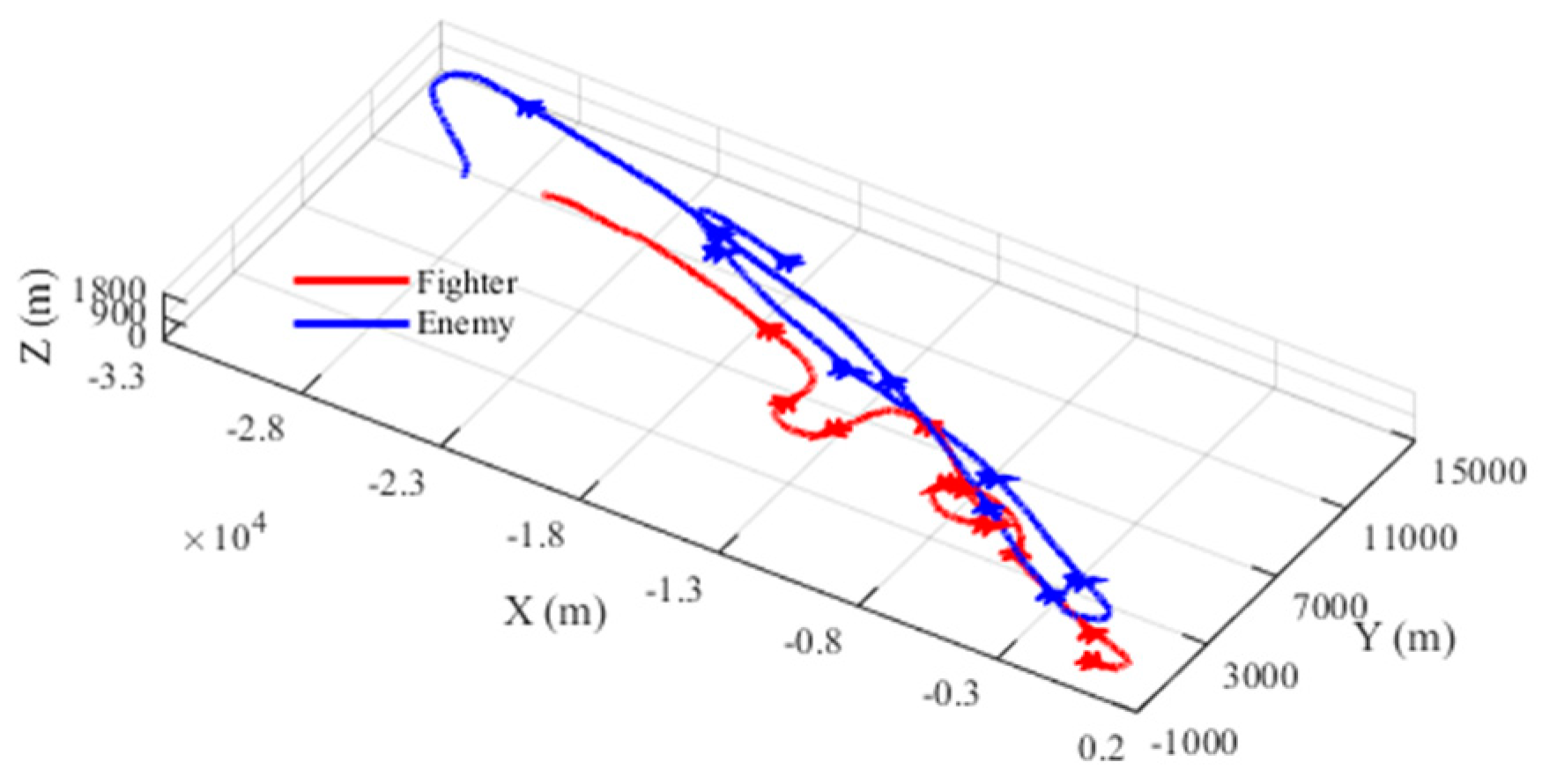
According to the description of relative situation information of the enemy and us in Section 2, based on the target position information obtained by the airborne radar sensor, the speed (value and angle), flight path angle, and heading angle of the target can be obtained by solving. On this basis, the target azimuth angle and entry angle can be further obtained. Therefore, the DWOSELM model can be used to accurately predict the maneuvering trajectory of the target and then the future air combat situation characteristic information of the target can be obtained through calculation. In this paper, a set of single machine confrontation trajectory data was extracted from the confrontation training system and used to verify the prediction performance of the DWOSELM model. The trajectory of the air combat confrontation is shown in Figure 13.
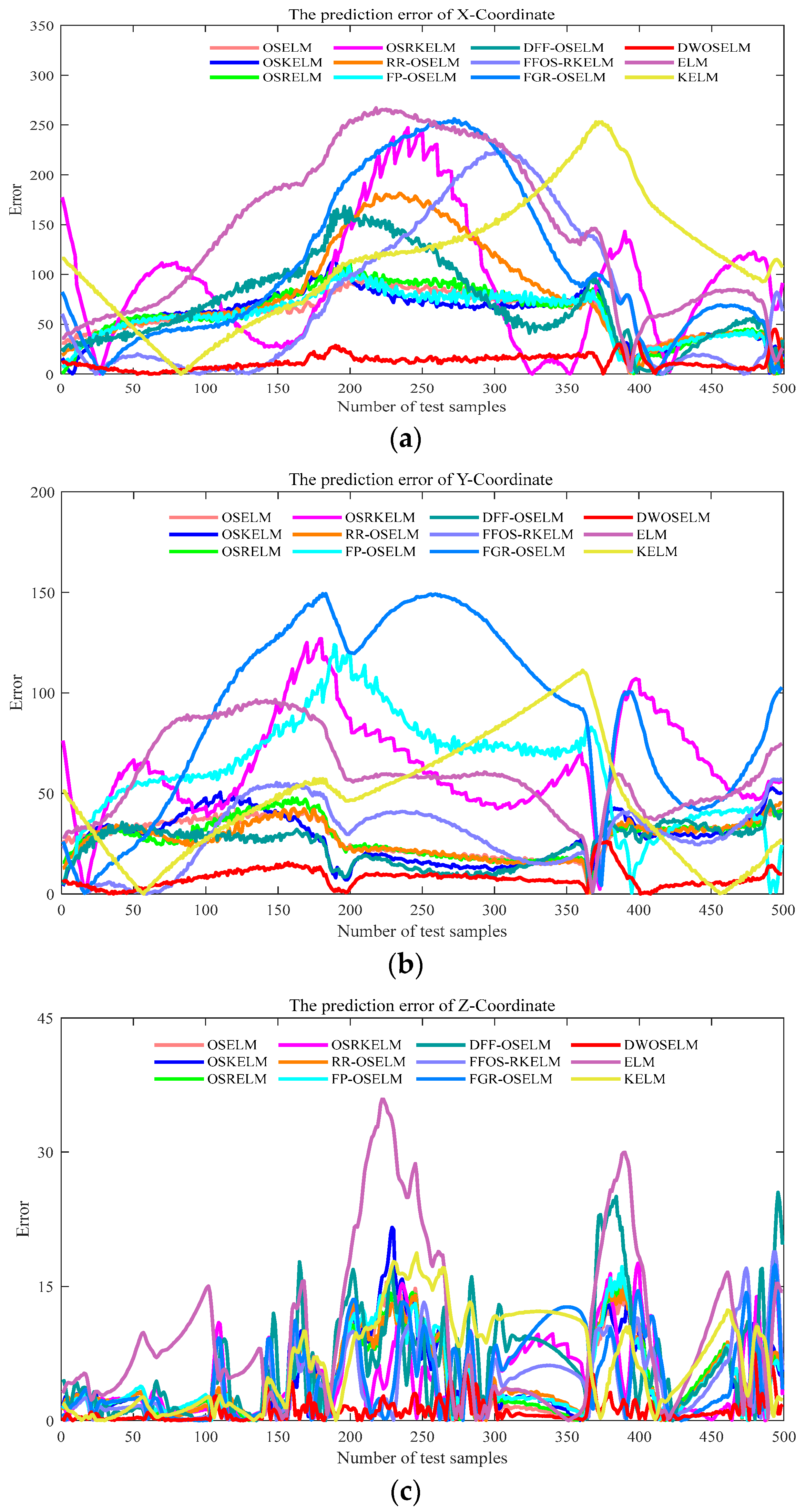
To reduce the contingency error of the prediction algorithm, the prediction result of each algorithm is the average result obtained from conducting 20 repeated experiments. The results of the single-step prediction of the target maneuver trajectories by the different algorithms are shown in Table 8. To more intuitively compare the prediction performance of different algorithms on the target maneuver trajectory, the absolute error values of single-step prediction of different algorithms are presented in the form of a figure, as shown in Figure 14.
Table 8 shows the prediction results of each algorithm on the target maneuver trajectory and the single-step prediction error of each algorithm is shown in Figure 14. It can be seen that, in terms of algorithm prediction accuracy, the DWOSELM prediction algorithm proposed in this paper has the smallest RMSE, MAD, MAPE, and NMSE. Under the same test data set, hardware platform, and initial parameter settings of the algorithm, its prediction accuracy is significantly better than that of other prediction methods in the literature. In terms of algorithm running time, the DWOSELM algorithm needs a little more running time due to the introduction of the sample dynamic weighting strategy, but it still meets the real-time requirements of the algorithm in the air combat decision-making process. To sum up, the air combat target maneuver trajectory prediction model based on the DWOSELM algorithm can accurately obtain the target’s future state information in real time, and then the future air combat situation information can be obtained.

7.3. Performance Verification of Air Combat Situation Assessment Model

To verify the performance of the DSASKEWO air combat situation assessment model proposed in this paper, this assessment model and the situation assessment based on missile attack area (SAMAA) model in [35] were, respectively, applied to medium-range air combat maneuver decision-making to test their effectiveness. The specific implementation scheme of the medium-range air combat maneuver decision-making method was as follows:
Step1: Based on the situation information between the enemy and us at the current time t, execute the control commands of all actions in the action library respectively and conduct maneuver exploration.
Step2: Predict all possible positions of our aircraft in the next stage through step1, solve the air combat situation between us and the enemy at each position, and obtain the air combat situation set S i t + Δ t = S A i , t + Δ t , S R i , t + Δ t , S H i , t + Δ t , η V i , t + Δ t at the next moment. A represents the number of maneuver actions, and the membership value set S t + Δ t = S 1 t + Δ t , S 2 t + Δ t , , S n t + Δ t , i = 1 , 2 , 3 , , n of the situation parameter variables corresponding to all maneuver actions.
Step3: Calculate the mean value and standard deviation of the set S i t + Δ t corresponding to the i t h maneuver, obtain the binary array M S i t + Δ t = m i t + Δ t , s i t + Δ t composed of m i t + Δ t and s i t + Δ t , form the set M Q t + Δ t = M S i t + Δ t , select the largest expected element in M Q t + Δ t , and take its corresponding maneuver action as the tactical action to be executed.
Step4: Time update, return to step1.
To fully illustrate the effectiveness of the air combat situation assessment method proposed in this paper, the DSASKEWO assessment method and the SAMAA assessment method were used, respectively, for the simple maneuver and some complex maneuvers of the enemy aircraft, and the air combat maneuver decision simulation experiment was conducted by combining the above maneuver decision methods. The air combat simulation experiment scenario is shown in Table 9.
(1)
Scenario 1
Scenario setting: The enemy aircraft is in the rear position of our fighter. The enemy aircraft adopts a constant speed maneuver, which initially forms the dominant position of the enemy.
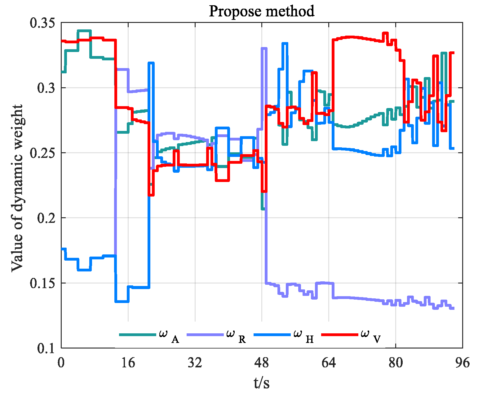
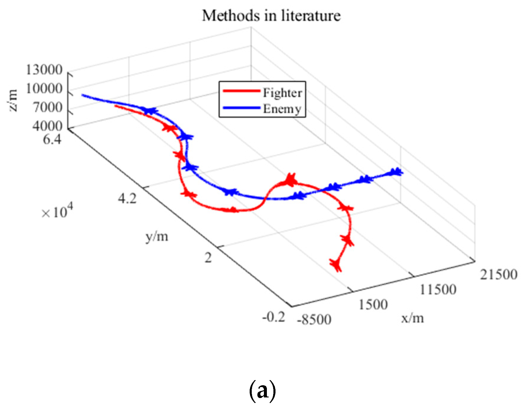
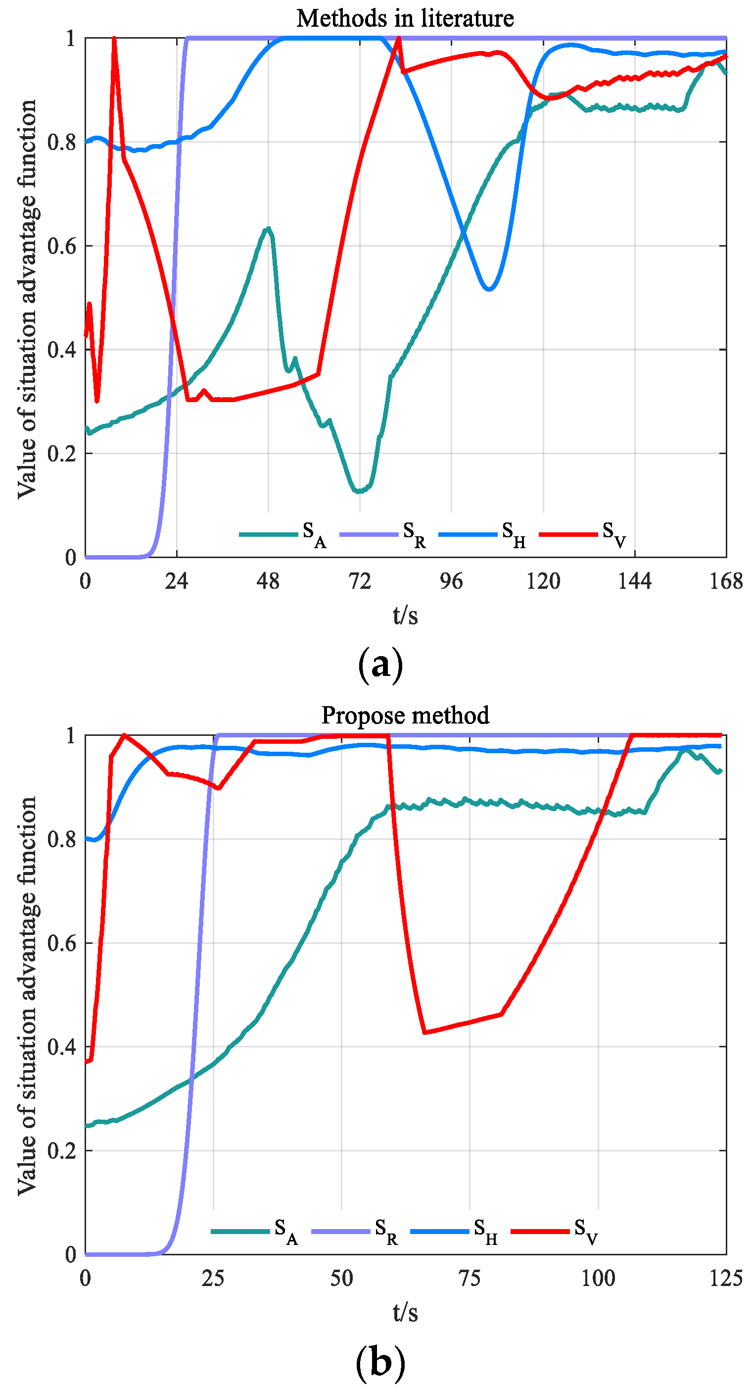
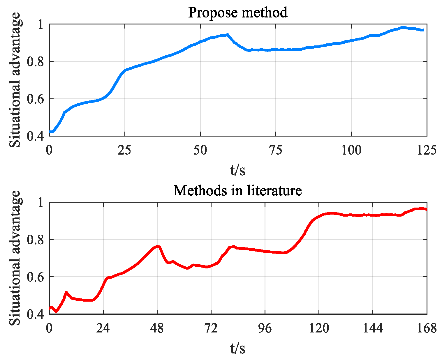
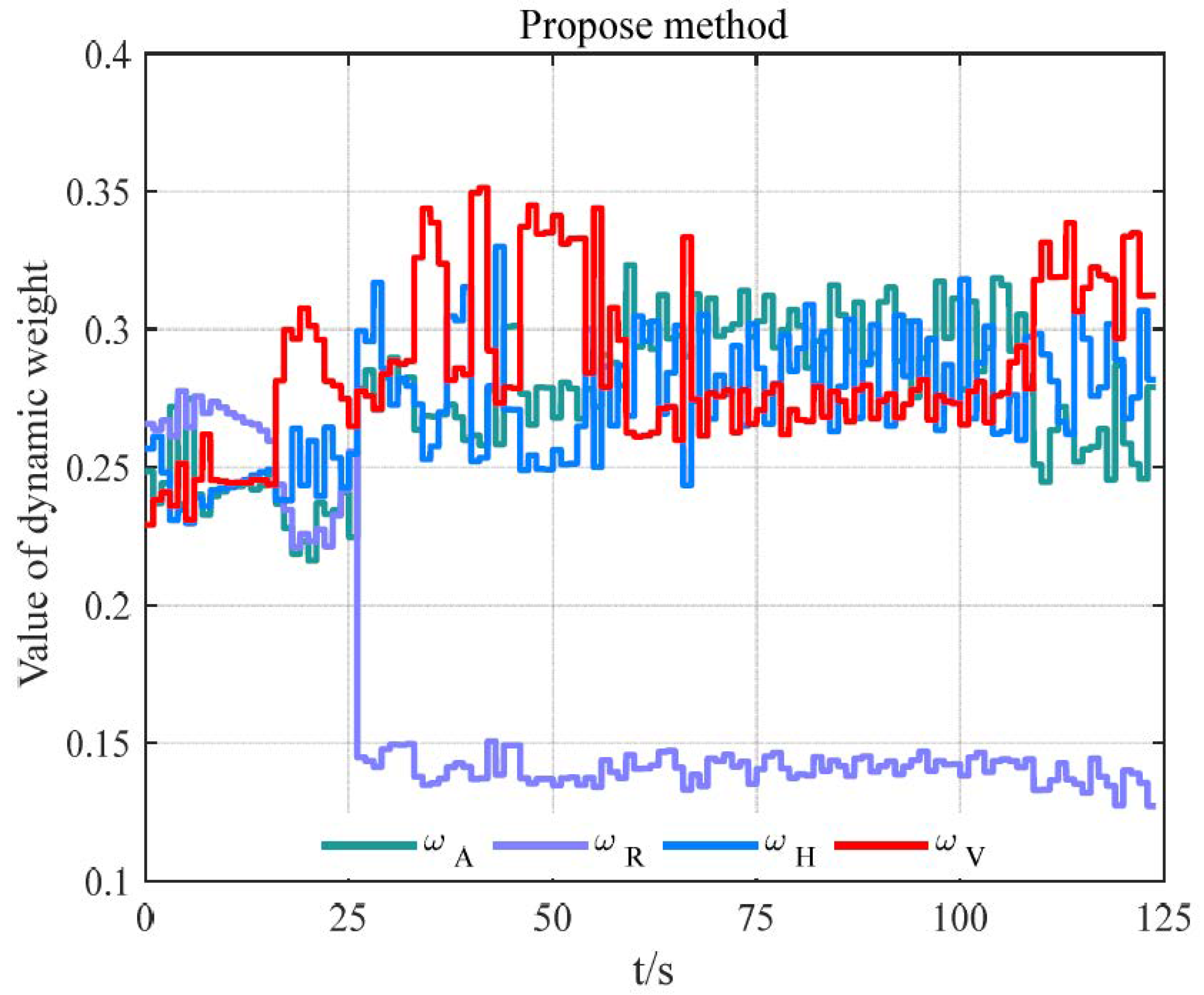
When we and the enemy formed the initial air combat situation of tail-chasing, different air combat situation assessment methods were used to conduct maneuver decision simulation experiments under the same initial conditions. The confrontation simulation results, the change curve of each situation advantage function value, the change curve of the comprehensive situation advantage function value, and the change curve of the situation advantage function index weight are shown in Figure 15, Figure 16, Figure 17 and Figure 18.
From the maneuver decision results shown in Figure 15, it can be seen that, to allow our fighter to obtain a greater attack-occupying advantage, the maneuver decision methods based on the two situation assessment models adopted a series of maneuver strategies to guide the fighter to form a tail-chasing situation relative to the enemy. The maneuver decision-making model based on SAMAA adopts the maneuver sequence of “right turn-climb-right dive-right turn-right climb-left dive-right turn-keep flight” to change the air combat situation from a disadvantage to an advantage, to obtain the occupying advantage against the enemy. However, the maneuver decision model based on DSASKEWO adopts a relatively simple maneuver sequence, which is “left dive-direct flight-left turn-direct flight”, and finally realizes the transformation from disadvantage to advantage. It shows that maneuver decision-making based on the air combat situation assessment model proposed in this paper can guide our fighter to complete maneuver dominance more quickly and accurately, thus accelerating the operational cycle of “Observation, Orientation, Decision, Action”, namely the OODA loop.
Through the analysis of the comprehensive situation advantage function and the change curve of each situation advantage function value, it can be seen that the changing trend of each parameter based on the DSASKEWO maneuver decision model is unchanged. Therefore, the load borne by the pilot is also small, which is conducive to the pilot controlling the fighter for air combat confrontation while reducing energy loss, avoiding unnecessary maneuvers, and being more conducive to our air combat victory.
To sum up, it can be seen that the performance of the air combat situation assessment model proposed in this paper is better. When our aircraft is in an unfavorable situation, it can quickly and accurately guide the carrier to maneuver to occupy a favorable situation.
(2)
Scenario 2
Scenario setting: The fighter meets the enemy in the front hemisphere and the enemy aircraft adopts snake maneuver strategy to form an initial situation of mutual disadvantage.
To fully verify the effectiveness of the air combat situation assessment method proposed in this paper, the maneuver decision verification experiment was conducted under the condition that the enemy conducts complex maneuvers. Assuming that the enemy aircraft performs a snake maneuver, under the initial situation of mutual disadvantage between us and enemy, different air combat situation assessment methods were used to conduct maneuver decision simulation experiments under the same initial conditions. The results of the confrontation simulation, the change curve of each situation advantage function value, the change curve of comprehensive situation advantage function value, and the change curve of situation advantage function index weight are shown in Figure 19, Figure 20, Figure 21 and Figure 22.
It can be seen from the two maneuver decision results shown in Figure 19 that, for the snake maneuver adopted by the enemy, the maneuver decision model based on SAMAA adopted the maneuver sequence of “left climb-left dive-right turn-left turn”, while the maneuver decision model based on DSASKEWO adopted the maneuver sequence of “left climb-flat flight”. It is obvious that the maneuver decision-making method based on the situation assessment model proposed in this paper can better deal with the maneuver strategy adopted by the target. According to the maneuver decision sequence, in the initial stage of decision-making, both methods perform left climbing maneuvers but the execution time is different. The SAMAA-based maneuver decision-making method takes too long to execute the left climb, which causes our aircraft to miss the opportunity to form a tail-chasing dominant situation, reducing the decision-making efficiency.
According to the change curves of the comprehensive situation advantage function values and the change curves of each situation advantage function values shown in Figure 20 and Figure 21, the maneuver decision method based on the DSASKEWO evaluation model is highly volatile, while the maneuver decision method based on the DSASKEWO evaluation model is relatively stable; especially in the later stage of the confrontation, the comprehensive situation advantage is stable and has obvious advantages. This fully demonstrates the rationality and effectiveness of the maneuver decision-making method based on the DSASKEWO evaluation model.
To sum up, when the enemy aircraft adopts complex maneuvers, the maneuver decision-making method based on the DSASKEWO evaluation model is more reasonable and effective, and can quickly and accurately guide the fighter to complete maneuver occupation and form an occupation advantage against the enemy.
8. Conclusions

Air combat situation assessment is the premise of decision-making and the key to intelligent air combat. With more and more information-based weapons being equipped, the amount of battlefield information has increased dramatically. How to use air combat data to evaluate the battlefield situation quickly and accurately has become an urgent problem to solve. Aiming at the shortcomings of current air combat situation assessment, a dynamic air combat situation assessment model based on situation knowledge extraction and weight optimization was proposed by combining a multiple regression model of hidden logic process, a weight optimization model based on grey prospect theory, a weight mapping model based on AE-ELM, and an air combat situation characteristic parameter prediction model based on DWOSELM. The model divides the medium-range air combat situation assessment into four steps, namely, air combat situation primitive extraction, situation assessment index weight optimization, air combat situation information prediction, and air combat situation assessment model construction. In this paper, taking the situation knowledge extraction and situation assessment of medium-range air combat as the research base point, the historical trajectory of air combat confrontation was transformed into the time series data of situation characteristic parameters, and the knowledge of the air combat situation was extracted by using a multivariate time series segmentation algorithm and a weight optimization algorithm. On this basis, the situation information prediction model, weight dynamic mapping model, and dynamic situation assessment model were constructed, which makes the air combat situation assessment model more practical.

Author Contributions

Conceptualization, Z.X.; Methodology, Z.X.; Software, Y.K.; Investigation, Z.X.; Data curation, Z.X.; Writing—original draft, Y.K.; Writing—review & editing, Y.L. (Yue Lv); Visualization, Y.K.; Supervision, Y.L. (You Li); Project administration, Z.L. All authors have read and agreed to the published version of the manuscript.

Funding

This document is supported by the National Natural Science Foundation of China (Project No. 72301293).

Data Availability Statement

Not applicaple.

Conflicts of Interest

The authors declare no conflict of interest.

References

  1. Gu, J.J.; Liu, W.H.; Jiang, W.Z. WVR air combat situation assessment model based on weapon engagement zone and kill probability. Syst. Eng. Electron. Technol. 2015, 37, 1306–1312. [Google Scholar]
  2. Shi, Z.Q.; Liang, X.L.; Zhang, J.Q.; Liu, L. Situation Assessment for Air Combat Based on Missile Attack Zone. Fire Control Command Control 2018, 43, 89–93. [Google Scholar]
  3. Zhou, S.; Wu, W.; Qu, Z.; Zhu, M. Analysis of Air Combat Situation Assessment Based on Nonparametric Methods. Aeronaut. Comput. Tech. 2011, 41, 13–16+20. [Google Scholar]
  4. Li, Z.W.; Chang, Y.Z.; Yang, H.Y.; Kou, Y.X.; Xu, A. Situation Assessment Method for Cooperative Air Combat Based on Dynamic Combat Power Field. J. Syst. Simul. 2015, 27, 1584–1590+1600. [Google Scholar]
  5. Cheng, T.F.; Ge, Q.B.; Chen, S.D.; Liu, B. Comparison of Weights Calculation Methods Based on Improved Air Combat Threat Assessment Model. Fire Control Command Control 2016, 41, 32–36. [Google Scholar]
  6. Ji, H.M.; Yu, H.; Song, S.; Peng, C.Q. Air Combat Situation Assessment Based on Improved Rough Set-cloud Model Theory. Tactical Missile Technol. 2019, 25, 20–27. [Google Scholar]
  7. Meng, X.F.; Du, H.W.; Feng, P.W. Study on situation assessment in air combat based on Gaussian cloudy Bayesian network. Comput. Eng. Appl. 2016, 52, 249–253. [Google Scholar]
  8. Shi, J.G.; Gao, X.G.; Li, X.M. Modeling Air Combat Situation Assessment by Using Fuzzy Dynamic Bayesian Network. J. Syst. Simul. 2006, 18, 1093–1096+1100. [Google Scholar]
  9. Jiang, L.T.; Kou, Y.N.; Wang, D.; Zhang, B.C. A dynamic variable weight method for situation assessment in close-range air combat. Electron. Opt. Control 2019, 26, 1–5. [Google Scholar]
  10. Zhao, K.X.; Huang, C.Q.; Wei, Z.L.; Wang, L. Situation assessment for unmanned aerial vehicle air combat based on anti-reasoning rules decision tree. J. Harbin Inst. Technol. 2019, 51, 66–73. [Google Scholar]
  11. Fan, J.; Lei, Y.J. Threat Assessment of Air Combat Based on RBF Neural Network. Microcomput. Inf. 2008, 24, 203–204. [Google Scholar]
  12. Huang, J.; Teng, P.; Zhang, B. Target Threat Assessing in Air Combat Based on Dynamic ANN Expert System. J. Proj. Rocket. Missiles Guid. 2004, S9, 518–520. [Google Scholar]
  13. Xiao, L.; Huang, J.; Xu, Z.S. Modeling air combat situation assessment based on combat area division. J. Beijing Univ. Aeronaut. Astronaut. 2013, 39, 1309–1313. [Google Scholar]
  14. Chang, Y.Z.; Li, Z.W.; Kou, Y.X.; Xu, A.; Yang, H.Y. Method for formation selection in air combat under uncertain information condition. Syst. Eng. Electron. 2016, 38, 2552–2560. [Google Scholar]
  15. Liu, S.F.; Dang, Y.G.; Fang, Z.G.; Xie, N.M. Grey System Theory and Its Application, 5th ed.; Science Press: Beijing, China, 2010; pp. 256–257. [Google Scholar]
  16. Hu, J.W.; Yin, Q.J.; Feng, L.; Deng, H.J.; Zha, Y.B. Research of CGF agent decision-making modeling based on prospect theory. J. Natl. Univ. Def. Technol. 2010, 32, 131–136. [Google Scholar]
  17. Zhang, K.; Zhang, Z.C.; Liu, Z.K.; Li, K.; Liu, B.B. Multi-target dynamic threat assessment in mixed air combat based on FD-TODIM algorithm. Syst. Eng. Electron. 2023, 45, 148–154. [Google Scholar]
  18. Chamroukhi, F.; Same, A.; Aknin, P.; Govaert, G. Model-based clustering with Hidden Markov Model regression for time series with regime changes. In Proceedings of the 2011 International Joint Conference on Neural Networks, San Jose, CA, USA, 31 July–5 August 2011; pp. 2814–2821. [Google Scholar]
  19. Chamroukhi, F.; Nguyen, H.D. Model-based clustering and classification of functional data. Wiley Interdiscip. Rev. Data Min. Knowl. Discov. 2019, 9, e1298. [Google Scholar] [CrossRef]
  20. Feng, Z.; Hodgings, J.K. Aligned cluster analysis for temporal segmentation of human motion. In Proceedings of the 2008 8th IEEE International Conference on Automatic Face & Gesture Recognition, Amsterdam, The Netherlands, 17–19 September 2008; pp. 1–7. [Google Scholar]
  21. Zhou, F.; De la Torre, F.; Hodgings, J.K. Hierarchical aligned cluster analysis for temporal clustering of human motion. IEEE Trans. Pattern Anal. Mach. Intell. 2012, 35, 582–596. [Google Scholar] [CrossRef]
  22. Lioutikov, R.; Neumann, G.; Maeda, G.; Peters, J. Learning movement primitive libraries through probabilistic segmentation. Int. J. Robot. Res. 2017, 36, 879–894. [Google Scholar] [CrossRef]
  23. Yu, C.C.; Wu, Z.J.; Tan, L.; Tu, X.Y.; Yang, Y.; Wang, L. Multivariate time series fuzzy clustering segmentation mining algorithm. J. Univ. Sci. Technol. Beijing 2014, 36, 260–265. [Google Scholar]
  24. Wang, G.X.; Hao, Y.S.; Su, Z.G. Condition diagnosis method for thermal power generation equipment based on KPCA-GG. J. Southeast Univ. (Nat. Sci. Ed.) 2019, 49, 542–548. [Google Scholar]
  25. Wang, L.; Xu, P.P.; Peng, K.X. Segmentation of multivariate time series with factor model and dynamic programming. Control Decis. 2020, 35, 35–44. [Google Scholar]
  26. Liang, N.Y.; Huang, G.B.; Saratchandran, P.; Sundararajan, N. A Fast and Accurate Online Sequential Learning Algorithm for Feedforward Networks. IEEE Trans. Neural Netw. 2006, 17, 1411–1423. [Google Scholar] [CrossRef] [PubMed]
  27. Deng, W.Y.; Ong, Y.S.; Tan, P.S.; Zheng, Q.H. Online sequential reduced kernel extreme learning machine. Neurocomputing 2016, 174, 72–84. [Google Scholar] [CrossRef]
  28. Huynh, H.T.; Won, Y. Regularized online sequential learning algorithm for single-hidden layer feedforward neural networks. Pattern Recognit. Lett. 2011, 32, 1930–1935. [Google Scholar] [CrossRef]
  29. Scardapane, S.; Comminiello, D.; Scarpiniti, M.; Uncini, A. Online sequential extreme learning machine with kernels. IEEE Trans. Neural Netw. Learn. Syst. 2014, 26, 2214–2220. [Google Scholar] [CrossRef]
  30. Guo, W.; Tang, K.M.; Yu, J.J. Robust Regularized Online Sequential Extreme Learning Machine for Outliers Restraining. J. Nanjing Univ. Aeronaut. Astronaut. 2019, 51, 7. [Google Scholar]
  31. Liu, D.; Wu, Y.X.; Jiang, H. FP-ELM: An online sequential learning algorithm for dealing with concept drift. Neurocomputing 2016, 207, 322–334. [Google Scholar] [CrossRef]
  32. Soares, S.G.; Araujo, R. An Adaptive Ensemble of On-line Extreme Learning Machines with Variable Forgetting Factor for Dynamic System Prediction. Neurocomputing 2015, 171, 693–707. [Google Scholar] [CrossRef]
  33. Jin, X.Z.; Zhang, S.K. Prediction of inlet NOx based on extreme learning machine of kernel mapping. Control Decis. 2019, 34, 213–218. [Google Scholar]
  34. Guo, W.; Xu, T.; Tang, K.M.; Yu, J.J. Online sequential extreme learning machine with generalized regularization and forgetting mechanism. Control Decis. 2017, 32, 247–254. [Google Scholar]
  35. Wu, W.H.; Zhou, S.Y.; Gao, L.; Liu, J.T. Improvements of situation assessment for beyond-visual-range air combat based on missile launching envelope analysis. Syst. Eng. Electron. 2011, 33, 2679–2685. [Google Scholar]
Figure 1. The relative geometric relationship between enemy and us.
Aerospace 10 00994 g001
Figure 2. The division of air combat situation space. (a) Advantages; (b) Mutual disadvantage; (c) Disadvantage; (d) Mutual safe.
Aerospace 10 00994 g002
Figure 3. The structure of air combat situation assessment model.
Aerospace 10 00994 g003
Figure 4. Autoencoder structure based on a three-layer feedforward neural network.
Aerospace 10 00994 g004
Figure 5. The schematic diagram of angle advantages. (a) k = 0.5; (b) k = 0.8.
Aerospace 10 00994 g005
Figure 6. The schematic diagram of distance advantages.
Aerospace 10 00994 g006
Figure 7. The schematic diagram of speed advantages. (a) Expected speed; (b) Speed advantage.
Aerospace 10 00994 g007aAerospace 10 00994 g007b
Figure 8. The schematic diagram of height advantages. (a) Expected height; (b) Height advantage.
Aerospace 10 00994 g008aAerospace 10 00994 g008b
Figure 9. The synthetic time series and real segmentation position. (a) Synthetic multivariate time series data 1; (b) Synthetic multivariate time series data 2.
Aerospace 10 00994 g009
Figure 10. The segmentation results of synthetic multivariate time series. (a) The segmentation result of synthetic multivariate time series data 1; (b) The segmentation result of synthetic multivariate time series data 2.
Aerospace 10 00994 g010
Figure 11. Air combat confrontation trajectory. (a) Air combat confrontation trajectory 1; (b) Air combat confrontation trajectory 2.
Aerospace 10 00994 g011
Figure 12. The segmentation results of air combat confrontation trajectory. (a) The segmentation results of air combat confrontation trajectory 1; (a) The segmentation results of air combat confrontation trajectory 1.
Aerospace 10 00994 g012
Figure 13. Air combat confrontation trajectory.
Aerospace 10 00994 g013
Figure 14. Comparison of one-step prediction errors of various algorithms. (a) Comparison of X coordinate single-step prediction error; (b) Comparison of Y coordinate single-step prediction error; (c) Comparison of Z coordinate single-step prediction error.
Aerospace 10 00994 g014
Figure 15. Maneuver decision results based on different assessment methods. (a) Maneuver decision results based on SAMAA situation assessment method; (b) Maneuver decision results based on DSASKEWO situation assessment method.
Aerospace 10 00994 g015
Figure 16. Change curve of each situation advantage function value based on different models. (a) Change curve of each situation advantage function value based on SAMAA model; (b) Change curve of each situation advantage function value based on DSASKEWO model.
Aerospace 10 00994 g016
Figure 17. Change curve of comprehensive situation advantage function value.
Aerospace 10 00994 g017
Figure 18. Change curve of indicator weight of situation advantage function.
Aerospace 10 00994 g018
Figure 19. Maneuver decision results based on different assessment methods. (a) Maneuver decision results based on SAMAA situation assessment method; (b) Maneuver decision results based on DSASKEWO situation assessment method.
Aerospace 10 00994 g019aAerospace 10 00994 g019b
Figure 20. Change curve of each situation advantage function value based on different models. (a) Change curve of each situation advantage function value based on SAMAA model; (b) Change curve of each situation advantage function value based on DSASKEWO model.
Aerospace 10 00994 g020
Figure 21. Change curve of comprehensive situation advantage function value.
Aerospace 10 00994 g021
Figure 22. Change curve of indicator weight of situation advantage function.
Aerospace 10 00994 g022
Table 1. Characteristic parameters of air combat situation.
Characteristic ParameterRangeCharacteristic ParameterRange
Relative distance R [0, 200]Azimuthal angle of fighter q f [0, π]
Relative height Δ H [0, 15,000]Azimuthal angle of target q e [0, π]
Velocity of our fighter v f [100, 500]Entrance angle of fighter φ f [0, π]
Velocity of target aircraft v e [100, 500]Entrance angle of target φ e [0, π]
Table 2. Confusion matrix.
PositiveNegative
Positive(True Positive, TP)(False Negative, FN)
Negative(False Positive, FP)(True Negative, TN)
Table 3. The segmentation results of different algorithms on synthetic multivariate time series 1.
AlgorithmPrecisionRecallAccuracySpecificityF1-ScoreGmean
MRHLP1.00001.00001.00001.00001.00001.0000
KPCA-GG0.87900.87470.89260.87720.98290.9357
FCM0.47450.71070.45880.53550.95670.5858
GMM0.62240.93830.70100.78210.98690.8172
k-means0.96100.95220.96190.95450.99460.9778
SC0.83820.92310.84670.87970.98630.9094
MHMMR0.84200.84830.84040.83310.97780.8996
MPWR0.19300.26350.24240.18420.88720.2893
ACA0.84020.86440.85330.84680.97720.9092
HACA0.89010.89620.89620.87930.98470.9371
Table 4. The segmentation results of different algorithms on synthetic multivariate time series 2.
AlgorithmPrecisionRecallAccuracySpecificityF1-ScoreGmean
MRHLP0.99100.99030.99230.99120.99820.9953
KPCA-GG0.88200.87080.91090.87510.97780.9422
FCM0.84620.99600.91130.94180.99930.9492
GMM0.84520.99600.90070.93750.99890.9442
k-means0.43260.47970.48830.48390.88410.5036
SC0.94910.94420.96400.94770.99040.9763
MHMMR0.89600.89890.89590.89180.97950.9352
MPWR0.80200.83360.84120.77700.96640.8932
ACA0.82620.82140.85230.82690.96620.9038
HACA0.94310.94360.94830.94240.98880.9679
Table 5. The results of different segmentation algorithms on air combat adversarial trajectory 1.
AlgorithmPrecisionRecallAccuracySpecificityF1-ScoreGmean
MRHLP0.9135 0.8980 0.8514 0.8685 0.9541 0.8978
KPCA-GG0.7741 0.6660 0.6427 0.6289 0.8889 0.6826
FCM0.7503 0.6397 0.5450 0.5539 0.8629 0.5618
GMM0.7546 0.7118 0.7375 0.6203 0.8908 0.7664
k-means0.7866 0.6477 0.6599 0.6487 0.8899 0.6523
SC0.7507 0.6308 0.6720 0.6298 0.8702 0.6836
MHMMR0.8132 0.7732 0.6735 0.6737 0.9074 0.7436
MPWR0.6760 0.4720 0.4269 0.4458 0.7532 0.3637
ACA0.8451 0.8040 0.6862 0.7120 0.9111 0.7648
HACA0.7539 0.6323 0.5658 0.5638 0.8623 0.5757
Table 6. The results of different segmentation algorithms on air combat adversarial trajectory 2.
AlgorithmPrecisionRecallAccuracySpecificityF1-ScoreGmean
MRHLP0.8897 0.8847 0.7955 0.8284 0.9567 0.8661
KPCA-GG0.8362 0.8261 0.7902 0.7623 0.9372 0.8450
FCM0.3529 0.2954 0.3811 0.2811 0.7940 0.4101
GMM0.7586 0.6264 0.5707 0.5821 0.9102 0.6132
k-means0.7654 0.6400 0.6102 0.6180 0.9092 0.6377
SC0.6816 0.5638 0.5740 0.5634 0.8794 0.6034
MHMMR0.7423 0.5645 0.6643 0.5826 0.9053 0.7281
MPWR0.6938 0.4832 0.5766 0.5204 0.8856 0.6115
ACA0.7951 0.8258 0.7205 0.7286 0.9187 0.7948
HACA0.7628 0.6392 0.6826 0.6466 0.9106 0.7324
Table 7. The algorithm parameter settings.
AlgorithmCore IdeasRegularization Parameter CKernel Parameter Other Parameters
OSELMRecursive least square method---
OSKELMkernel learning method-1000-
OSRELM regularization technique 10 × 105 -
OSRKELMkernel learning method, regularization technique10 × 1051000-
RR-OSELMPriori error inverse weighting, regularization technique10 × 105--
FP-OSELMforgetting factor, regularization technique10 × 105- α = r a n d
DFF-OSELMforgetting factor, regularization technique-- λ 0 = 1 , γ 0 = 10 3 v 0 = 10 6 , ρ = 0.99
FFOS-RKELMkernel learning, forgetting factor, regularization technique10 × 1051000 λ 0 = 1 , γ 0 = r a n d v 0 = r a n d , ρ = 3.8
FGR_OSELMforgetting factor, regularization technique10 × 105- λ = 0.98
RTrOS-VolterraRobustness, transfer learning, Tikhonov regularization technique10 × 10--
Table 8. Single-step prediction results of the target maneuver trajectory.
Target TrajectoryAlgorithmRMSEMADMAPENMSEPTAS/sPTPS/s
X-CoordinateOSELM62.722959.10160.00374.7838 × 10−50.03390.00007
OSKELM64.234059.61580.00375.0171 × 10−50.94560.00189
OSRELM67.348661.72170.00385.4769 × 10−50.03340.00007
OSRKELM112.284192.86070.00581.5270 × 10−40.19260.00039
RR-OSELM93.291679.14820.00461.0583 × 10−40.03540.00007
FP-OSELM63.154458.59410.00364.8499 × 10−50.03450.00007
DFF-OSELM82.786071.00270.00448.3337 × 10−50.03810.00008
FFOS-RKELM107.113776.07500.00351.3896 × 10−41.12330.00225
FGR-OSELM134.7634108.51150.00572.1996 × 10−40.46160.00093
DWOSELM14.044412.15406.5198 × 10−42.3890 × 10−60.31380.00063
ELM161.7131140.87250.00823.0809 × 10−40.02790.00006
KELM130.7593115.68810.00622.0039 × 10−40.06640.00013
Y-CoordinateOSELM29.863228.55960.00341.0254 × 10−40.03030.00006
OSKELM30.302227.99120.00331.0558 × 10−40.92370.00185
OSRELM29.637828.20070.00321.0100 × 10−40.03250.00007
OSRKELM68.205763.95290.00685.2986 × 10−40.19820.00040
RR-OSELM28.435927.14830.00319.2974 × 10−50.03420.00007
FP-OSELM67.281162.04610.00395.5044 × 10−50.03490.00007
DFF-OSELM25.871224.20010.00287.6959 × 10−50.03400.00007
FFOS-RKELM32.780028.80900.00291.2239 × 10−41.13360.00227
FGR-OSELM100.068289.59100.00870.00110.44750.00090
DWOSELM9.02977.76267.9835 × 10−49.2867 × 10−60.31080.00062
ELM62.495259.00850.00674.2042 × 10−40.02820.00006
KELM57.766446.35300.00473.1996 × 10−40.06490.00013
Z-CoordinateOSELM6.06034.39640.00573.6207 × 10−40.03270.00007
OSKELM6.26954.62950.00603.8749 × 10−40.95330.00191
OSRELM6.00784.44510.00583.5582 × 10−40.03150.00006
OSRKELM6.38674.89120.00604.0101 × 10−40.19890.00040
RR-OSELM6.05914.59070.00593.6193 × 10−40.03600.00007
FP-OSELM6.18074.61380.00603.7659 × 10−40.03420.00007
DFF-OSELM8.69386.60510.00807.4510 × 10−40.03750.00008
FFOS-RKELM5.78584.29260.00513.2911 × 10−41.12030.00225
FGR-OSELM6.66975.07110.00604.4128 × 10−40.45360.00091
DWOSELM1.62661.08710.00132.6012 × 10−50.30920.00062
ELM13.21829.79870.01330.00170.02770.00006
KELM8.35186.54600.00746.7669 × 10−40.06510.00013
Note: processing time on all samples (PTAS) and per sample (PTPS).
Table 9. Initial air combat situation scenario.
Simulation NumberCombatUnitInitial ConditionSituationTarget Maneuver
x 0 / m y 0 / m z 0 / m v 0 ( m / s ) Ψ 0 / ( ° ) γ 0 / ( ° )
1P007500360−1350disadvantageconstant speed maneuver
T20,00020,0006000320−1350
2P008000320450mutual disadvantageS maneuver
T20,00020,0009000360−900
Disclaimer/Publisher’s Note: The statements, opinions and data contained in all publications are solely those of the individual author(s) and contributor(s) and not of MDPI and/or the editor(s). MDPI and/or the editor(s) disclaim responsibility for any injury to people or property resulting from any ideas, methods, instructions or products referred to in the content.