Development of a Controlled Dynamics Simulator for Reusable Launcher Descent and Precise Landing

Abstract

This paper introduces a Reusable Launch Vehicle (RLV) descent dynamics simulator coupled with closed-loop guidance and control (G&C) integration. The studied vehicle’s first-stage booster, evolving in the terrestrial atmosphere, is steered by a Thrust Vector Control (TVC) system and planar fins through gain-scheduled Proportional–Integral–Derivative controllers, correcting the trajectory deviations until precise landing from the reference profile computed in real time by a successive convex optimisation algorithm. Environmental and aerodynamic models that reproduce realistic atmospheric conditions are integrated into the simulator for enhanced assessment. Comparative performance results were achieved in terms of control configuration (TVC-only, fins-only, and both) for nominal conditions as well as with external disturbances such as wind gusts or multiple uncertainties through a Monte Carlo analysis to assess the G&C system. These studies demonstrated that the configuration combining TVC and steerable planar fins has sufficient control authority to provide stable flight and adequate uncertainties and disturbance rejection. The developed simulator provides a preliminary assessment of G&C techniques for the RLV descent and landing phase, along with examining the interactions that occur. In particular, it paves the way towards the development and assessment of more advanced and robust algorithms.

1. Introduction

Over the last decade, launcher reusability has become the new paradigm for reducing the cost of access to space and enabling future manned missions, such as a return to the Moon or, even more ambitiously, the first steps on Mars. This technology was already developed in the Space Shuttle era; however, unanticipated costs and risks led to the cancellation of the programme in 2011. Nevertheless, some years ago, private companies, such as SpaceX and Blue Origin, completely disrupted the space sector and demonstrated the cost effectiveness and technical feasibility of reusable rockets. More specifically, SpaceX’s Falcon 9 became in 2017 the first Vertical Take-Off Vertical Landing (VTVL) vehicle, having its first stage recovered after launch and reused for another mission, and then became in 2020 the first private rocket to take astronauts to the International Space Station thanks to its spacecraft Dragon [1]. Today, SpaceX has flown reusable boosters more than 100 times, with some single boosters reused more than 10 times, proving the feasibility and economic sustainability of such a technology. This leading company is now successfully testing its Super Heavy rocket equipped with the Starship spacecraft with the objective of carrying both crew and cargo on long-duration interplanetary flights, achieving humanity’s return to the Moon, and travelling to Mars and beyond. Meanwhile, Blue Origin is also developing advanced reusable launchers such as New Shepard, a suborbital launch vehicle designed for space tourism, and New Glenn, a heavy-lift reusable rocket that should be able to carry heavy payloads to Earth’s orbit and beyond [2]. Consequently, national agencies and intergovernmental institutions are following the same path, increasing research and development related to launcher reusability.

The descent and precision soft-landing of Reusable Launch Vehicles (RLVs) on Earth are very challenging, mainly due to the presence of the atmosphere. Indeed, during this phase, the vehicle is subjected to fast system dynamics changes induced by external loads such as lift and drag, unpredictable wind gusts, and control-induced actuation commands to comply with the landing requirements, allowing so-called pinpoint landing while preserving the vehicle’s integrity. All of these factors involve uncertainties and nonlinearities, which lead to vehicle instability and therefore justify the implementation of a high-performance guidance, navigation, and control (GNC) system. A solution to this demanding problem became feasible in the past decade with the development of convex optimisation: a particular class of methods that allow one to compute, in real time and based on the current flight conditions, optimal trajectories to be followed satisfying the desired constraints (which must be convex). This technology was demonstrated by the Masten Space Systems’ VTVL demonstrator Xombie, which used a vision-based system and a fuel-optimal convex guidance algorithm for precision landing [3].

Research on convex optimisation for the entry, descent, and soft pinpoint landing of VTVL reusable launchers has actively been carried out in recent years with the development of advanced techniques such as successive convex optimisation [4] and pseudospectral convex optimisation [5,6]. In Ref. [7], Liu extended this first method by combining aerodynamic forces and propulsion as control inputs to gain optimality with the consideration of vehicle aerodynamics, which had previously been ignored. Then, in Ref. [8], Sagliano et al. combined both methods and proposed separating the aerodynamic descent and powered landing into two different optimal control problems, using aerodynamic forces as the control input for the first phase and a combination of aerodynamic and propulsive control for the second phase. Finally, in Ref. [9], Simplício et al. solved a simplified optimal control problem in a first step and passed the solution to a second step involving successive convex optimisation to include aerodynamic effects.

The coupled flight mechanics involved in the reusable launcher descent and landing (D&L) phase are in fact usually not considered in the design of optimal guidance algorithms. The disturbances and uncertainties acting on the vehicle and arising from the nonlinear dynamics; external events (e.g., wind and aerodynamics); the actuation system; and the environment are counteracted by a properly designed robust control system. Classic techniques involve the use of linear control theory based on linearising the equations of motion and feedback of defined control parameters with gain scheduling [10]. However, these techniques require an extensive verification and validation campaign with Monte Carlo analyses, which render the process very time-consuming and costly. Lately, advanced robust control methods have been studied in both academia and industry, such as the Linear Parameter-Varying (LPV) approach [11] and the $H_{\infty }$ family of methods, specifically the structured $H_{\infty }$ technique [12].

The steering of a VTVL reusable rocket during the D&L phase is generally achieved by a Thrust Vector Control (TVC) system, which actuates by deflecting the engine nozzle along the two body axes perpendicular to the vehicle’s longitudinal axis through specific gimbal angles computed using the guidance and control (G&C) algorithms. To increase the control authority of the RLV, especially at low thrust during aerodynamic descent, steerable fins are crucial. They are typically placed above the vehicle’s centre of pressure, with one pair usually applied for controlling the pitch motion and another pair for controlling the yaw motion. Finally, a Reaction Control System (RCS) based on cold gas thrusters is often added for use at a high altitude in low-dynamic-pressure conditions or to provide roll control capabilities.

To understand the interactions between G&C and D&L flight mechanics, an RLV controlled dynamics simulator is proposed herein. This could serve as a baseline for the design and analysis of more advanced G&C methods for the D&L phase of reusable launchers. It covers the descent and soft pinpoint landing of a VTVL vehicle first-stage booster with closed-loop guidance and control integration. It includes the six-degrees-of-freedom (6-DoF) descent dynamics of a rigid-body model with a varying mass, evolving in the terrestrial atmosphere with varying environmental parameters, uncertainties, and disturbances (atmospheric density, ambient pressure, and wind) and subjected to external forces (gravity and aerodynamics). The steering of the spacecraft is carried out by a TVC system and planar fins, correcting the trajectory deviations with respect to the reference profile. The G&C system consists of a successive convex optimisation guidance algorithm updated several times during the flight and a control system composed of gain-scheduled Proportional–Integral–Derivative (PID) controllers. The main contributions of the proposed work can be summarised as follows:

• The development of a 6-DoF RLV controlled dynamics simulator with closed-loop guidance and control integration for the descent and precise landing phase. This tool allows one to assess G&C methods for realistic scenarios, more specifically with respect to environmental models (aerodynamics, wind, and atmospheric parameters) and the actuation system (TVC and steerable planar fins). Moreover, it has a modular architecture and therefore can be easily modified to integrate more complex models (e.g., propulsion and aerodynamics). To the best of the authors’ knowledge, such a simulator is not publicly available and therefore provides the opportunity to understand the challenges involved in designing G&C algorithms for reusable launcher descent and precise landing and perform preliminary assessments of multiple recovery strategies.
• The implementation and assessment of a successive convex optimisation guidance algorithm that solves the 6-DoF equations of motion for the powered descent and pinpoint landing problem.
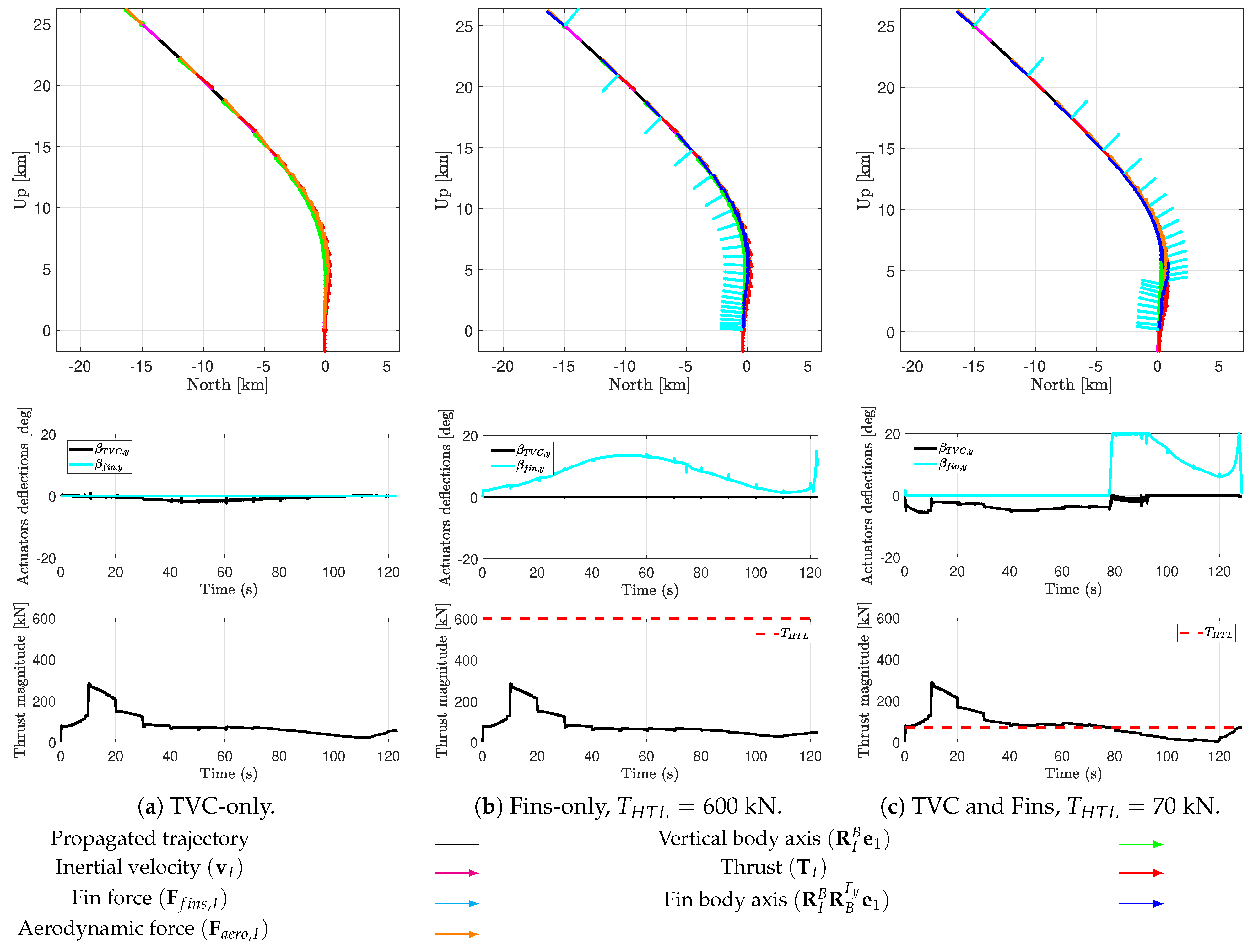
• The generation of corrections using classical linear feedback control through gain-scheduled PID controllers. Then, commands are allocated between the TVC system and the steerable planar fins according to the level of thrust. This feature also allows a certain modularity for studying different actuation configurations according to the mission requirements (e.g., propellant consumption) and the flight phase: TVC-only, planar fins-only, or both.

The paper is organised as follows. Section 2 introduces the reusable launcher controlled dynamics simulator with a description of all the building blocks: from the reference frames, environmental and aerodynamic models, and vehicle dynamics to the definition of the different actuation systems. Then, the successive convex optimisation guidance algorithm is introduced in Section 3. In addition, Section 4 presents the preliminary control method using classic linear control theory with gain-scheduled PID controllers and explains how the command is then allocated to the TVC system and/or the steerable planar fins. Subsequently, several simulations are performed in Section 5 with different actuation configurations. A sensitivity analysis is also carried out, adding wind and dispersion to several parameters in order to study their impact on the D&L performance and better address them for future developments in advanced G&C methods. Finally, conclusions are provided in Section 6.

2. Reusable Launcher Controlled Dynamics Modelling

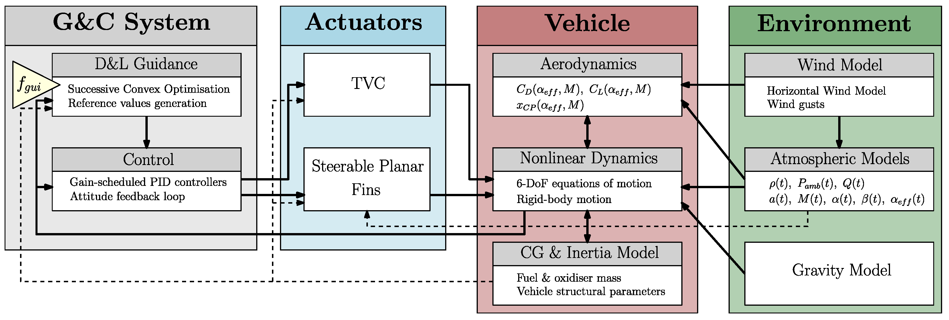
The RLV controlled dynamics simulator developed in this paper relies on the nonlinear 6-DoF dynamics of a VTVL vehicle first-stage booster modelled as a rigid body with a varying mass subjected to external forces induced by the terrestrial atmosphere and controlled through embedded closed-loop guidance and control strategies. Therefore, it is made up of several building blocks with interconnections. A description of the developed architecture is provided in Figure 1. The elements were implemented through MATLAB/Simulink R2021b and will be briefly presented in the following subsections. A performance analysis of the simulator described below with a simplified aerodynamic model and TVC actuation only was carried out in Ref. [13].

The reference frames and environmental models adopted for gravity, atmospheric parameters, and wind are explained in Section 2.1. Then, the equations of motion and the centre of gravity (CG) and inertia estimations are described in Section 2.2. The developed aerodynamic model is presented in Section 2.3. The vehicle is steered via TVC and planar fins depending on their level of control authority. These actuators are introduced in Section 2.4 and Section 2.5, respectively.

Finally, the G&C algorithms are organised into two subsystems. First, “D&L Guidance” is responsible for the real-time generation of the reference control values, here in terms of thrust magnitude and attitude angles. Note that this feature is executed at frequency $f_{gui}$, which differs from the simulator time step. A dedicated passage on the development of the guidance algorithm is provided in Section 3. Then, the “Control” subsystem, responsible for the computation of the commands allocated among the aforementioned actuators, is defined in Section 4.

2.1. Reference Frames and Environmental Models

This subsection describes the reference frames and environmental models that are adopted in the RLV controlled dynamics simulator. They are essential to simulating the re-entry of a reusable rocket into the terrestrial atmosphere.

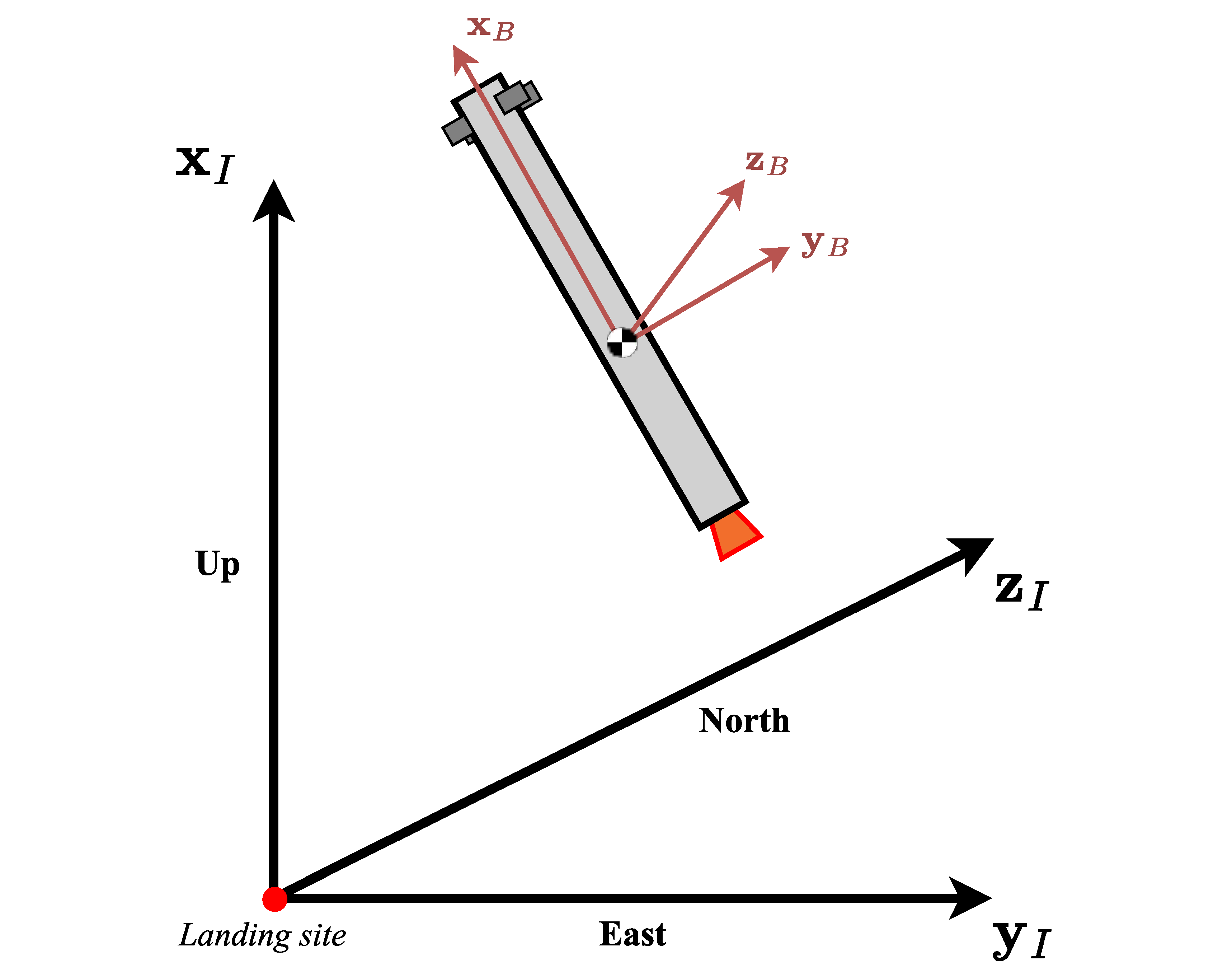
Two reference frames are considered and are shown in Figure 2. The first is the landing-site-centred reference frame. Its origin is at the landing site and it is an up–east–north reference frame, such that the ${\mathbf{x}}_I$-axis points up, the ${\mathbf{y}}_I$-axis east, and the ${\mathbf{z}}_I$-axis north. This reference frame is considered inertial, and the equations of motion refer to it. Simulations start from an initial position in this reference frame ${\mathbf{r}}_I\left(0\right)$, with an initial velocity ${\mathbf{v}}_I\left(0\right)$. The second reference frame is the vehicle’s body-fixed reference frame. This is fixed to the vehicle’s CG, and the basis vectors can be defined as follows: the ${\mathbf{x}}_B$-axis lies along the vehicle’s longitudinal axis, the ${\mathbf{y}}_B$-axis is defined so as to remain perpendicular to the pitch plane, and the ${\mathbf{z}}_B$-axis completes the right-handed system (and thus remains perpendicular to the yaw plane). Following these definitions, the roll, pitch, and yaw angles ($\varphi \left(t\right)$, $\theta \left(t\right)$, and $\psi \left(t\right)$, respectively) represent the orientation of the body-fixed reference frame with respect to the landing-site-centred inertial reference frame. These angles are useful for controlling the vehicle trajectory. However, in the formulation of the equations of motion, the rotation quaternion ${\mathbf{q}}_B^I\left(t\right)$ is used to translate the attitude of the vehicle. Therefore, ${\mathbf{R}}_B^I\left(t\right)$ represents the rotation matrix from the inertial reference frame to the vehicle’s body-fixed reference frame. The angular velocity is defined in the body-fixed reference frame with an initial value ${\mathit{\omega }}_B\left(0\right)$.

The atmosphere model adopted in this study, available in the MATLAB Aerospace Toolbox [14], implements the mathematical representation of the 1976 Committee on Extension to the Standard Atmosphere (COESA) [15], which provides, as a function of altitude $h\left(t\right)$, the atmospheric density $\rho \left(h\right(t\left)\right)$, the speed of sound $a\left(h\right(t\left)\right)$, and the ambient atmospheric pressure $P_{amb}\left(h\left(t\right)\right)$. Then, the gravitational field is defined in the inertial frame by ${\mathbf{g}}_I\left(h\left(t\right)\right)={\left[\begin{array}{ccc}g\left(h\right(t\left)\right)& 0& 0\end{array}\right]}^T$, where $g\left(h\right(t\left)\right)$ is obtained as a function of the altitude and expressed by

$$g\left(h\left(t\right)\right)=g_0{\left(\frac{R_E}{R_E+h\left(t\right)}\right)}^2$$

(1)

Here, $g_0\approx 9.81\mathrm{m}/{\mathrm{s}}^2$ is the standard gravity of Earth, and $R_E=6378\mathrm{km}$ is the radius of the Earth. For conciseness, these values will now be written as a function of time t.

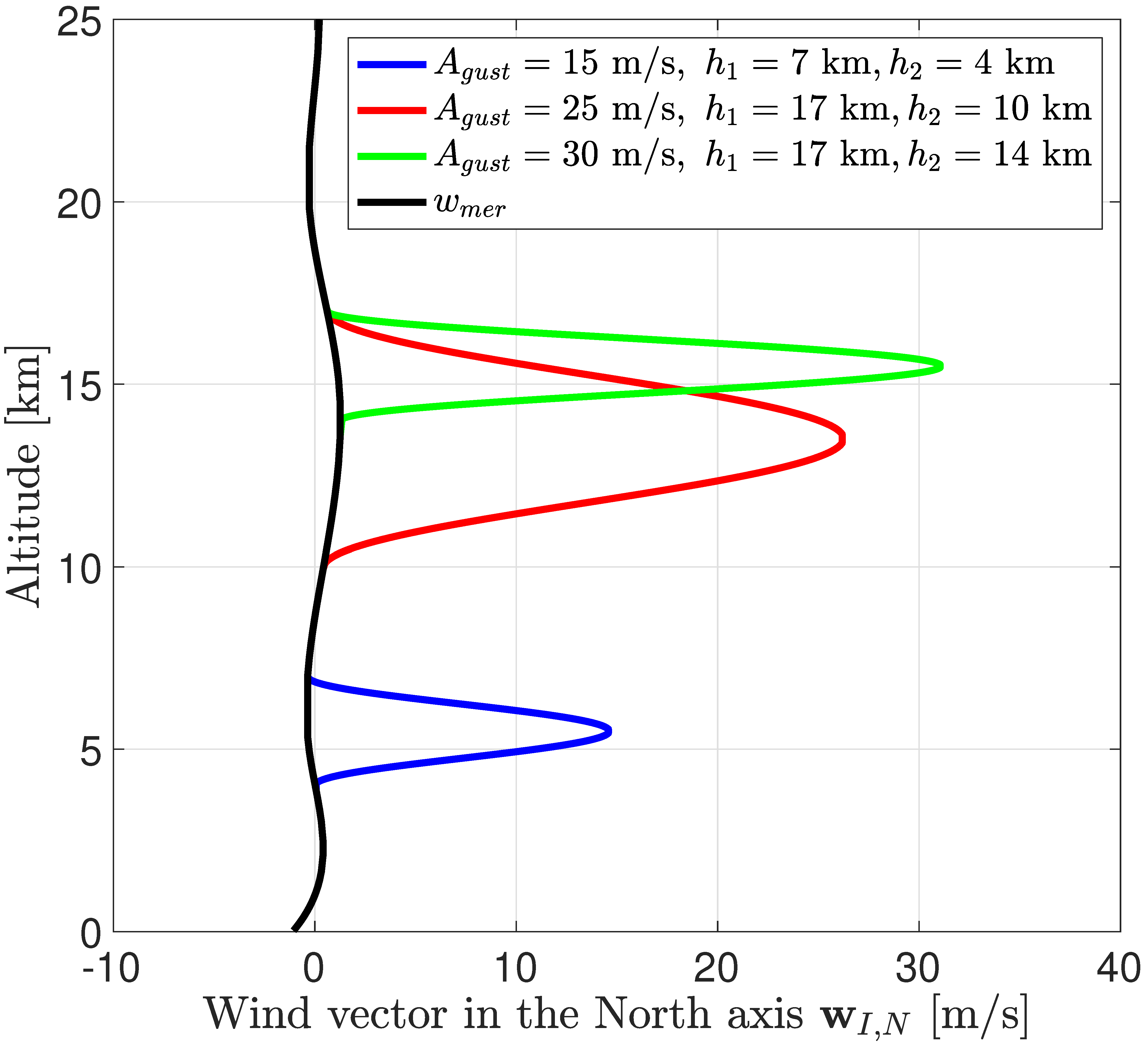
Finally, the constant wind is computed with the US Naval Research Laboratory model Horizontal Wind Model 14, also available in Ref. [14], which generates the meridional $w_{mer}\left(t\right)$ and zonal $w_{zon}\left(t\right)$ components of the wind for a set of geophysical data. Wind gusts are modelled as a cosine-shaped function, so the user can define the amplitude of the gust and the altitude at which it occurs. The function is expressed as follows:

$${\mathbf{V}}_{gust}\left(h\left(t\right)\right)=\left(\frac{{\mathbf{A}}_{gust}}{2}\right)\left(1-cos\left(\frac{\pi (h\left(t\right)-h_1)}{0.5\Delta h}\right)\right)$$

(2)

where ${\mathbf{A}}_{gust}\in {\mathbb{R}}^3$ specifies the amplitude of the gust in three directions, $h\left(t\right)$ is the current altitude of the spacecraft, $h_1$ specifies the altitude at which the gust starts, and $\Delta h$ is the altitude range in which the gust is applied. Therefore, the maximum intensity of the gust is reached in the middle of the specified altitude region. Consequently, the wind vector is written in the inertial reference frame as follows:

$${\mathbf{w}}_I\left(t\right)={\left[\begin{array}{ccc}0& w_{mer}\left(t\right)& w_{zon}\left(t\right)\end{array}\right]}^T+{\mathbf{V}}_{gust}\left(h\left(t\right)\right).$$

(3)

Note that the wind model is not considered in the descent dynamics of the guidance algorithm described in Section 3.

2.2. Equations of Motion and CG/Inertia Estimations

The equations of motion are written using the reference frames previously defined in Section 2.1. They are based on ${\mathbf{x}}_I\left(0\right)=\left[\begin{array}{ccccc}m\left(0\right)& {\mathbf{r}}_I^T\left(0\right)& {\mathbf{v}}_I^T\left(0\right)& {\mathbf{q}}_B^I{\left(0\right)}^T& {\mathit{\omega }}_B^T\left(0\right)\end{array}\right]$, the initial state vector, and the assumption that the vehicle is a rigid body with no effects induced by the varying mass (e.g., propellant sloshing) and structural flexibility.

The mass depletion dynamics are modelled by an affine function of the thrust magnitude as follows:

$$\dot{m}\left(t\right)=-\frac{\left|\right|{\mathbf{F}}_{TVC,I}\left(t\right){\left|\right|}_2}{I_{sp}{g}_0}-\frac{A_{nozzle}{P}_{amb}\left(t\right)}{I_{sp}{g}_0}$$

(4)

where $I_{sp}=282\mathrm{s}$ is the vacuum specific impulse of the engine, which is assumed to be constant for simplicity, and $A_{nozzle}=3.1416{\mathrm{m}}^2$ is the nozzle exit area of the engine. ${\mathbf{F}}_{TVC,I}\left(t\right)\in {\mathbb{R}}^3$ is the thrust vector coming from the TVC system, introduced in Section 2.4. The second term is related to the reduction in the specific impulse due to the atmospheric back pressure [4].

The translational states, position, and velocity of the vehicle in the inertial reference frame, ${\mathbf{r}}_I\left(t\right)\in {\mathbb{R}}^3$ and ${\mathbf{v}}_I\left(t\right)\in {\mathbb{R}}^3$, are governed by the following dynamics:

$$\begin{array}{cc}\hfill {\dot{\mathbf{r}}}_I\left(t\right)& ={\mathbf{v}}_I\left(t\right)\hfill \\ \hfill {\dot{\mathbf{v}}}_I\left(t\right)& =\frac{1}{m\left(t\right)}\left[{\mathbf{F}}_{TVC,I}\left(t\right)+{\mathbf{F}}_{aero,I}\left(t\right)+{\mathbf{F}}_{fins,I}\left(t\right)\right]+{\mathbf{g}}_I\left(t\right)\hfill \end{array}$$

(5)

where ${\mathbf{F}}_{aero,I}\left(t\right)\in {\mathbb{R}}^3$ describes the aerodynamic force acting on the vehicle in the inertial reference frame (Section 2.3), and ${\mathbf{F}}_{fins,I}\left(t\right)\in {\mathbb{R}}^3$ represents the control force generated by the planar fins (Section 2.5).

Then, the attitude states are governed by the following rotational dynamics, using the quaternion-based kinematics equation:

$$\begin{array}{cc}\hfill & {\dot{\mathbf{q}}}_B^I\left(t\right)=\frac{1}{2}\left[\begin{array}{ccc}{q}_4\left(t\right)& -q_3\left(t\right)& q_2\left(t\right)\\ q_3\left(t\right)& q_4\left(t\right)& -q_1\left(t\right)\\ -q_2\left(t\right)& q_1\left(t\right)& q_4\left(t\right)\\ -q_1\left(t\right)& -q_2\left(t\right)& -q_3\left(t\right)\end{array}\right]{\mathit{\omega }}_B\left(t\right)\hfill \\ \hfill & {\dot{\mathit{\omega }}}_B\left(t\right)=J^{-1}\left(t\right)\left[{\mathbf{M}}_{TVC,B}\left(t\right)+{\mathbf{M}}_{aero,B}\left(t\right)+{\mathbf{M}}_{fins,B}\left(t\right)-{\mathit{\omega }}_B\left(t\right)\times J{\mathit{\omega }}_B\right]\hfill \end{array}$$

(6)

where $J\left(t\right)$ is the inertia matrix of the vehicle, introduced below. ${\mathbf{M}}_{aero,B}\left(t\right)\in {\mathbb{R}}^3$, ${\mathbf{M}}_{TVC,B}\left(t\right)\in {\mathbb{R}}^3$, and ${\mathbf{M}}_{fins,B}\left(t\right)\in {\mathbb{R}}^3$ (Section 2.3, Section 2.4 and Section 2.5) represent the aerodynamic and control torques acting on the vehicle. In Equation (6), the coupling between angular velocity and inertia along the three axes and the effect of centroid movement on the inertia caused by mass consumption are ignored.

Finally, because of the propellant mass and the level variations throughout the flight, the total vehicle CG and the moments of inertia also vary. The CG is considered to lie along the vehicle body’s longitudinal axis, i.e., ${\mathbf{x}}_{CG}\left(t\right)={\left[\begin{array}{ccc}{x}_{CG}\left(t\right)& 0& 0\end{array}\right]}^T$, while the inertia tensor is assumed to be diagonal, i.e., $J\left(t\right)=\mathrm{diag}\left(\left[\begin{array}{ccc}{J}_A\left(t\right)& J_N\left(t\right)& J_N\left(t\right)\end{array}\right]\right)$. Following the model and data available in Ref. [16], the vehicle’s mass is broken down into structural mass and time-dependent propellant mass, which is updated via Equation (4) during engine burn. Therefore, the reader is referred to Ref. [16] for details of the parameters defining the inertial and CG properties and their numerical values.

2.3. Aerodynamic Model

The aerodynamic forces and moments generated by the vehicle depend on its structure, as well as the instantaneous dynamic pressure. This atmospheric parameter is usually given by

$$Q\left(t\right)=\frac{1}{2}\rho \left(t\right)V^2\left(t\right)$$

(7)

where $V\left(t\right)=\left|\right|{\mathbf{v}}_{air,I}\left(t\right){\left|\right|}_2$ and ${\mathbf{v}}_{air,I}\left(t\right)={\mathbf{v}}_I\left(t\right)-{\mathbf{w}}_I\left(t\right)$ are the air-relative velocity vectors written in the inertial reference frame that account for the wind ${\mathbf{w}}_I\left(t\right)$.

For the computation of aerodynamic loads, it is common to define a velocity reference frame that is fixed to the vehicle’s CG but directed along the air-relative velocity written in the body-fixed reference frame ${\mathbf{v}}_{air,B}\left(t\right)$. This reference frame enables the definition of the two aerodynamic angles, the angle of attack $\alpha \left(t\right)$ and the sideslip angle $\beta \left(t\right)$, in order to illustrate the rotation from the body-fixed to the velocity reference frame ${\mathbf{R}}_V^B\left(t\right)$, as follows:

$${\mathbf{R}}_V^B\left(t\right)=\left[\begin{array}{ccc}cos\alpha \left(t\right)cos\beta \left(t\right)& sin\beta \left(t\right)& sin\alpha \left(t\right)cos\beta \left(t\right)\\ -cos\alpha \left(t\right)sin\beta \left(t\right)& cos\beta \left(t\right)& -sin\alpha \left(t\right)sin\beta \left(t\right)\\ sin\alpha \left(t\right)& 0& cos\alpha \left(t\right)\end{array}\right]$$

(8)

where the aerodynamic angles are given by

$$\begin{array}{cc}\hfill \alpha \left(t\right)& =atan2(v_{air,B,z}\left(t\right),v_{air,B,x}\left(t\right))\hfill \\ \hfill \beta \left(t\right)& =arcsin\left(\frac{v_{air,B,y}\left(t\right)}{V\left(t\right)}\right).\hfill \end{array}$$

(9)

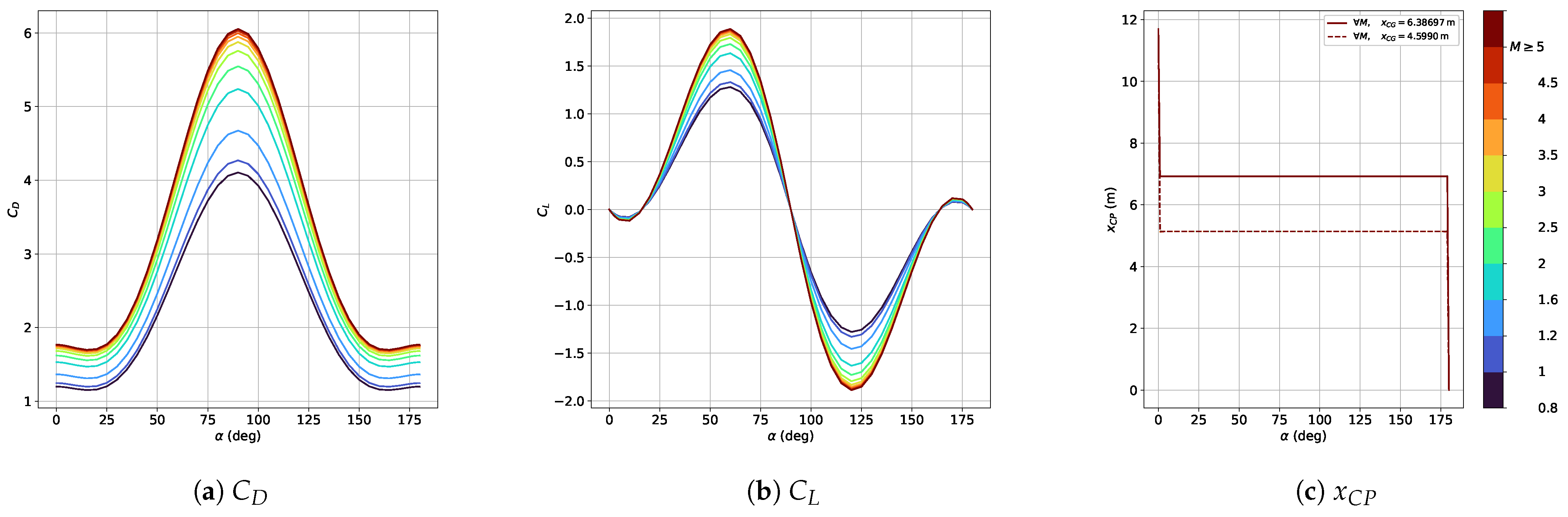
With these definitions and assuming that the vehicle has an axisymmetric shape, the aerodynamic forces and moments generated by the vehicle are expressed in the body-fixed reference frame as

$$\begin{array}{cc}\hfill {\mathbf{F}}_{aero,B}\left(t\right)& =-Q\left(t\right)S_{ref}{\mathbf{R}}_B^V\left(t\right)\left[\begin{array}{c}{C}_D({\alpha }_{eff}\left(t\right),M\left(t\right))\\ 0\\ C_L({\alpha }_{eff}\left(t\right),M\left(t\right))\end{array}\right]\hfill \\ \hfill {\mathbf{M}}_{aero,B}\left(t\right)& =\left[{\mathbf{x}}_{CP}\left(t\right)-{\mathbf{x}}_{CG}\left(t\right)\right]\times {\mathbf{F}}_{aero,B}\left(t\right)\hfill \end{array}$$

(10)

where $S_{ref}=7.14{\mathrm{m}}^2$ is the vehicle reference area; ${\mathbf{x}}_{CP}\left(t\right)={\left[\begin{array}{ccc}{x}_{CP}\left(t\right)& 0& 0\end{array}\right]}^T$ is the vehicle’s center of pressure (CP); and $\{C_D,C_L\}$ are the drag and lift coefficients, respectively. These parameters are estimated as functions of the effective angle of attack ${\alpha }_{eff}\left(t\right)=\sqrt{{\alpha }^2\left(t\right)+{\beta }^2\left(t\right)}$ and the Mach number $M\left(t\right)=V\left(t\right)/a\left(t\right)$, where $a\left(t\right)$ is the speed of sound, also obtained from COESA as a function of altitude.

Aerodynamic parameters are obtained using the Supersonic/Hypersonic Arbitrary-Body Program (S/HABP) for a cylindrical-shape first-stage rocket, with an angle of attack from 0 to 180 deg and a Mach number from 0.8 to 5. This programme, which was developed in 1973 by the United States Air Force Flight Dynamics Laboratory [17] and used by the National Aeronautics and Space Administration, has been adapted to obtain an aerodynamic database composed of the aerodynamic coefficients and the CP as function of the Mach number and the aerodynamic angles. More details on the development of the aerodynamic database and its validation are given in Ref. [18]. These coefficients are then linearly interpolated in the simulator according to the current flight conditions. The variation of $C_D$, $C_L$ and $x_{CP}$ with respect to ${\alpha }_{eff}\left(t\right)$ and $M\left(t\right)$ is illustrated in Figure 3.

Note that this aerodynamic database has some limitations. In fact, S/HABP was designed to operate from about Mach 2 to the hypersonic range [19]. However, for the RLV descent phase, and particularly for this study, the Mach number range starts around Mach 5 and then drops below Mach 1 until reaching zero velocity at landing. In addition, the aerodynamic coefficients are assumed to be independent of the thrust level. This approximation is very rough for retro-propulsive flight, where there are significant interactions between the exhaust plume of the engine and the oncoming flow that substantially impact the drag coefficient and the heat loads [20]. Therefore, the approximations obtained for the aerodynamic coefficients might diverge from the true values [18]. However, the goal of this simulator is not to gather high-fidelity models but to study the interactions and challenges that exist in the design of an RLV controlled dynamics simulator and assess the advanced and robust G&C methods that must be developed accordingly.

2.4. TVC System

The trajectory of the vehicle during descent is controlled by adjusting the magnitude and direction of the thrust vector generated by the main engine. This is achieved by the TVC actuator deflecting the engine nozzle by ${\beta }_{TVC,y}\left(t\right)$ and ${\beta }_{TVC,z}\left(t\right)$, respectively, along the ${\mathbf{y}}_B$-axis and ${\mathbf{z}}_B$-axis. The required thrust magnitude $T_{ref}\left(t\right)$ and deflection angles $\{{\beta }_{TVC,y}\left(t\right),{\beta }_{TVC,z}\left(t\right)\}$ are obtained from the guidance algorithm (Section 3) and the control method (Section 4), respectively. Decoupling between translational and rotational dynamics is common for TVC control due to the fact that the attitude of the vehicle can change faster than its trajectory [16]. Thus, the TVC-generated force and moment can be expressed in the body-fixed frame by

$$\begin{array}{cc}\hfill {\mathbf{F}}_{TVC,B}\left(t\right)& =T_{ref}\left(t\right)\left[\begin{array}{c}cos\left({\beta }_{TVC,y}\left(t\right)\right)cos\left({\beta }_{TVC,z}\left(t\right)\right)\\ cos\left({\beta }_{TVC,y}\left(t\right)\right)sin\left({\beta }_{TVC,z}\left(t\right)\right)\\ -sin\left({\beta }_{TVC,y}\left(t\right)\right)\end{array}\right]\hfill \\ \hfill {\mathbf{M}}_{TVC,B}\left(t\right)& =\left[{\mathbf{x}}_{PVP}-{\mathbf{x}}_{CG}\left(t\right)\right]\times {\mathbf{F}}_{TVC,B}\left(t\right)\hfill \end{array}$$

(11)

where ${\mathbf{x}}_{PVP}={\left[\begin{array}{ccc}{x}_{PVP}& 0& 0\end{array}\right]}^T$ is the TVC pivot position ($x_{PVP}=0.96\mathrm{m}$).

2.5. Steerable Planar Fins Model

The implementation of planar fins for a G&C strategy has already been studied in the literature. Usually, two pairs of fins are placed above the vehicle’s CG: one pair, with deflections $\{{\beta }_{fin,1}\left(t\right),{\beta }_{fin,2}\left(t\right)\}$, controlls the motion in the pitch plane, while the other, with $\{{\beta }_{fin,3}\left(t\right),{\beta }_{fin,4}\left(t\right)\}$, controlls the motion in the yaw plane. Therefore, it is considered that there is no roll perturbation, meaning that the two pairs always remain in the trajectory yaw and pitch planes, respectively. In Ref. [8], Sagliano et al. used aerodynamic coefficient lookup tables that directly considered the state of the vehicle (angle of attack $\alpha \left(t\right)$, sideslip angle $\beta \left(t\right)$, and Mach number $M\left(t\right)$) and fin deflections $\{{\beta }_{fin,1}\left(t\right),{\beta }_{fin,2}\left(t\right),{\beta }_{fin,3}\left(t\right),{\beta }_{fin,4}\left(t\right)\}$. In Ref. [21], the authors developed a fin model with a corresponding lookup table for the axial coefficient and the derivative of the normal coefficient, depending on only the Mach number. Therefore, the lookup tables were the same for the four fins, and the generated force was determined by the fin’s local angle of attack, defined as a function of the fin deflection and the vehicle’s angle of attack or sideslip angle. Finally, in Ref. [16], Simplício et al. also developed a fin model, but it only considered the normal force, which was calculated as a function of the fin’s local angle of attack. The same approach is used in this paper, and the obtained planar fins model was validated in Ref. [22].

Table 1. Position of the fins’ CP with respect to the base of the RLV and corresponding deflections.

	Fin CP Position ${\mathbf{x}}_{\mathit{fin},\mathit{i}}$	Fin Deflection ${\mathit{\beta }}_{\mathit{fin},\mathit{i}}\left(\mathit{t}\right)$
Fin1	${\left[\begin{array}{ccc}{x}_{fin}& y{z}_{fin}& 0\end{array}\right]}^T$	${\beta }_{fin,1}\left(t\right)$
Fin2	${\left[\begin{array}{ccc}{x}_{fin}& -y{z}_{fin}& 0\end{array}\right]}^T$	${\beta }_{fin,2}\left(t\right)$
Fin3	${\left[\begin{array}{ccc}{x}_{fin}& 0& y{z}_{fin}\end{array}\right]}^T$	${\beta }_{fin,3}\left(t\right)$
Fin4	${\left[\begin{array}{ccc}{x}_{fin}& 0& -y{z}_{fin}\end{array}\right]}^T$	${\beta }_{fin,4}\left(t\right)$

defines the fin positions with the corresponding deflections.

Furthermore, due to the reduced fin area compared to the RLV body, only the normal force contribution is considered [16]. Then, the value of the normal coefficient of the fin is estimated using lifting-line theory [23]. In fact, for a symmetric airfoil, the lift coefficient can be approximated by

$$c_l\left(\alpha \left(t\right)\right)=2\pi \alpha \left(t\right).$$

(12)

To obtain the lift coefficient $C_L$ of the corresponding wing, it is necessary to define the aspect ratio, denoted by $AR$ and defined as

$$AR=\frac{b^2}{S}=\frac{b}{c}$$

(13)

where b is the wing span, S is the wing reference area, and c is the wing chord. Therefore, the following approximation is obtained [24]:

$$C_L\left(\alpha \left(t\right)\right)=\left(\frac{AR}{AR+2}\right)c_l\left(\alpha \left(t\right)\right).$$

(14)

This theory is then adapted for the fins of the RLV. Because flow separation is neglected and the angle of attack of the rocket is around $\pi$ during descent, the normal fin coefficient has a sinusoidal dependence on the fin angle of attack ${\gamma }_{fin,i}\left(t\right)$ and can be approximated by

$$C_{N,fin,i}\left({\gamma }_{fin,i}\left(t\right)\right)=2\pi \left(\frac{A{R}_{fin}}{A{R}_{fin}+2}\right)sin\left({\gamma }_{fin,i}\left(t\right)\right),i=\{1,2,3,4\}.$$

(15)

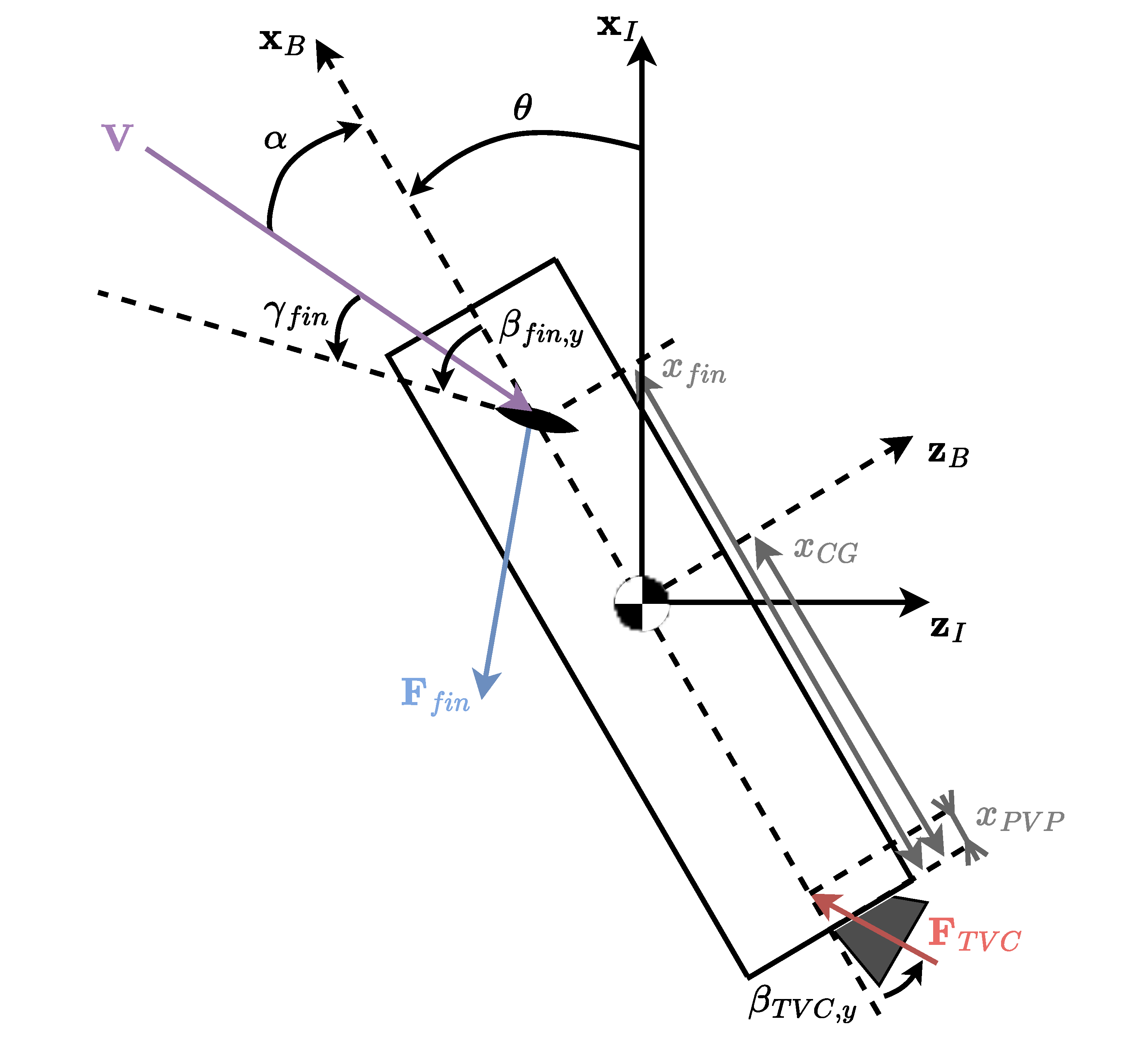
It remains to define the ith fin’s angle of attack and its associated force ${\mathbf{F}}_{fin,i}\left(t\right)$ and moment ${\mathbf{M}}_{fin,i}\left(t\right)$ in the vehicle’s body-fixed reference frame. Figure 4 shows the motion of the vehicle in the pitch plane; from this figure and Ref. [16], it is possible to state the following:

$$\left\{\begin{array}{c}{\gamma }_{fin,i}\left(t\right)={\beta }_{fin,i}\left(t\right)-\alpha \left(t\right)\hfill \\ {\mathbf{F}}_{fin,i}\left(t\right)=\frac{1}{2}\rho \left(t\right)\left|\right|{\mathbf{v}}_{air,I}\left(t\right){\left|\right|}_2^2{S}_{fin}{C}_{N,fin,i}\left({\gamma }_{fin,i}\left(t\right)\right){\left[\begin{array}{ccc}-sin\left({\beta }_{fin,i}\left(t\right)\right)& 0& cos\left({\beta }_{fin,i}\left(t\right)\right)\end{array}\right]}^T\hfill \\ {\mathbf{M}}_{fin,i}\left(t\right)=[{\mathbf{x}}_{fin,i}-{\mathbf{x}}_{CG}]\times {\mathbf{F}}_{fin,i}\left(t\right)\hfill \end{array}\right.,i=\{1,2\}$$

(16)

where $\alpha \left(t\right)$ is the vehicle’s angle of attack, and $S_{fin}$ is the fin reference area. Similarly, the following formula is obtained in the yaw plane:

$$\left\{\begin{array}{c}{\gamma }_{fin,i}\left(t\right)=-{\beta }_{fin,i}\left(t\right)-\beta \left(t\right)\hfill \\ {\mathbf{F}}_{fin,i}\left(t\right)=\frac{1}{2}\rho \left(t\right)\left|\right|{\mathbf{v}}_{air,I}\left(t\right){\left|\right|}_2^2{S}_{fin}{C}_{N,fin,i}\left({\gamma }_{fin,i}\left(t\right)\right){\left[\begin{array}{ccc}sin\left({\beta }_{fin,i}\left(t\right)\right)& cos\left({\beta }_{fin,i}\left(t\right)\right)& 0\end{array}\right]}^T\hfill \\ {\mathbf{M}}_{fin,i}\left(t\right)=[{\mathbf{x}}_{fin,i}-{\mathbf{x}}_{CG}]\times {\mathbf{F}}_{fin,i}\left(t\right)\hfill \end{array}\right.,i=\{3,4\}$$

(17)

where $\beta \left(t\right)$ is the vehicle’s sideslip angle.

Finally, the total force generated by the fixed planar fins in the inertial reference frame and the total moment generated in the vehicle’s body-fixed reference frame are given by

$${\mathbf{F}}_{fins,I}\left(t\right)={\mathbf{R}}_I^B\left(t\right)\sum _{i=1}^4{\mathbf{F}}_{fin,i}\left(t\right)$$

(18)

$${\mathbf{M}}_{fins,B}\left(t\right)=\sum _{i=1}^4{\mathbf{M}}_{fin,i}\left(t\right)$$

(19)

Table 2. Planar fins’ model parameters.

Parameter	Value	Unit
$x_{fin}$	$11.1$	$\mathrm{m}$
$y{z}_{fin}$	$2.5$	$\mathrm{m}$
$b_{fin}$	$1.2$	$\mathrm{m}$
$c_{fin}$	$0.8$	$\mathrm{m}$
$S_{fin}$	$0.96$	${\mathrm{m}}^2$
$A{R}_{fin}$	$1.5$	-

specifies the parameters of the planar fins that are implemented in the simulator.

3. Guidance Strategy

For the RLV D&L simulator introduced in the previous section, the guidance algorithm is responsible for the real-time generation of a reference trajectory to be followed by the vehicle with thrust and attitude commands. Here, a direct method is used within the convex optimisation framework. This consists in transforming the fuel-optimal trajectory problem into a convex one—more precisely, into a Second-Order Cone Programming (SOCP) problem, which can be solved with efficient solvers in polynomial time. These challenging tasks rely on converting nonconvex state and control constraints into the convex form, requiring high computational power. Recently, the so-called lossless convexification method [25] and advances in computational development have enabled these issues to be overcome and therefore allow real-time trajectory generation in a closed-loop fashion.

Moreover, a particular class of convex optimisation, successive convex optimisation, can be applied to approximate the remaining nonlinearities in the optimal landing problem, such as the aerodynamic effects, which have previously been ignored. This consists in iteratively solving convex optimisation SOCP subproblems in which the nonconvex dynamics and constraints are repeatedly linearised using information originating from the previous iteration’s solution. This algorithm was first developed by Szmuk et al. in Ref. [4] and then adapted in different ways in Refs. [7,9]. In this paper, the successive convex optimisation algorithm relies on the work achieved by Guadagnini et al. in Ref. [26], where the strategy defined in Ref. [4] was improved to be applicable in a closed-loop fashion for a 6-DoF controlled dynamics simulator.

In this study, the successive convex optimisation guidance algorithm is implemented in MATLAB using the CVX library [27] to formulate the convex problem and the ECOS routine [28] to solve it. At each simulation instance defined by the simulation rate $f_{sim}$, the reference thrust profile ${\mathbf{T}}_{B,ref}\left(t\right)$ and the reference attitude angles $\{{\theta }_{ref}\left(t\right),{\psi }_{ref}\left(t\right)\}$ are calculated from the most recent guidance solution by linear interpolation. 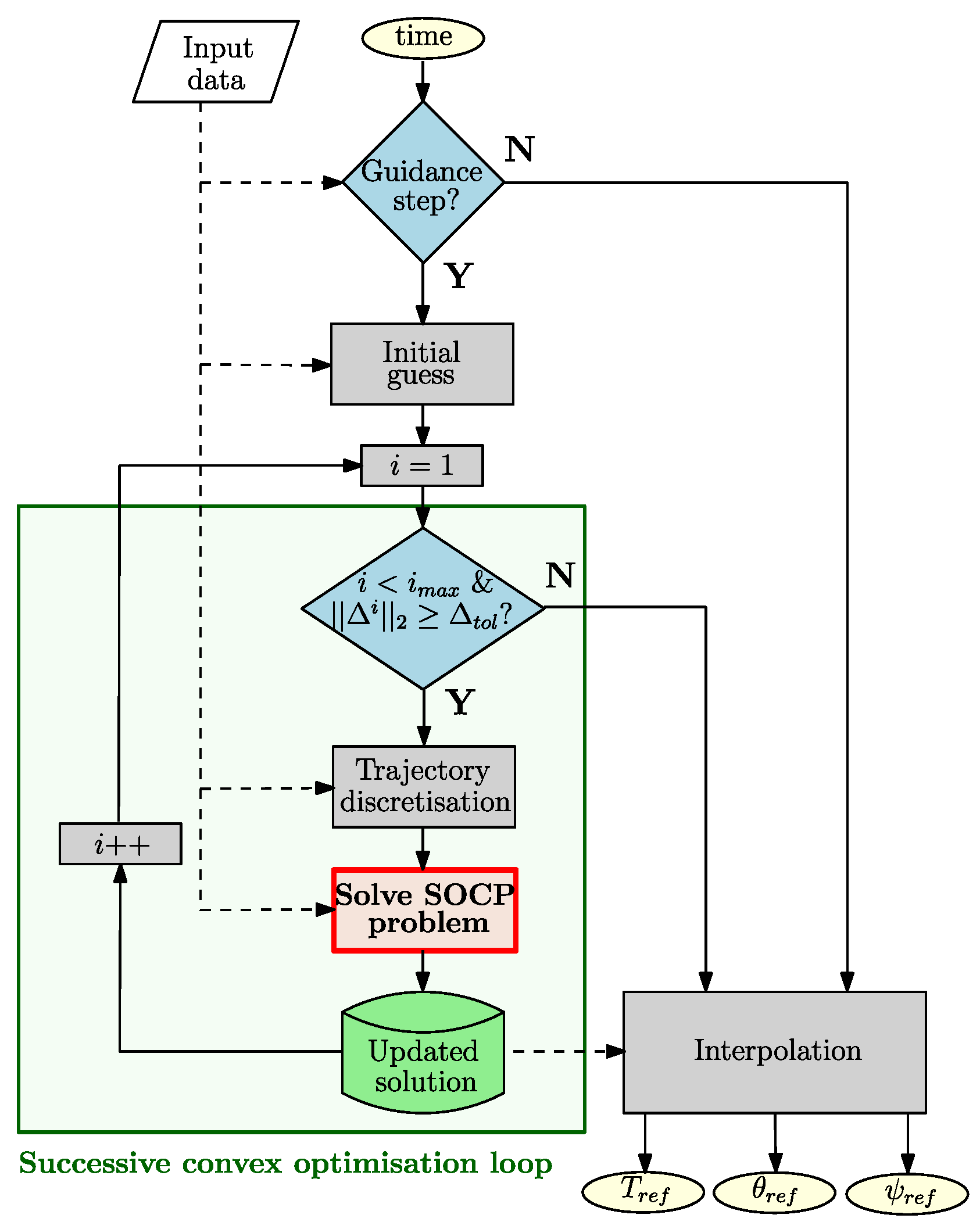In fact, this solution is stored as an online lookup table, which is updated at each guidance step, with the guidance update frequency $f_{gui}=0.1$ Hz, that is, every 10 s. The guidance algorithm inside the “D&L Guidance” building block of the simulator (recall Figure 1) is schematised in Figure 5.

Before describing the algorithm, a description of the adopted notation is provided. In the following paragraphs and subsections, the discrete time instant is specified with the parameter k. Consequently, a variable a at the time instant k is represented as $a\left[k\right]$. Then, since we are handling an iterative process, the considered iterative solution is specified with the superscript i. Therefore, the solution a obtained at iteration i is specified as $a^i$. Thus, a variable a at a time instant k, relative to iteration i, is denoted $a^i\left[k\right]$.

First, it is necessary to initialise the process with a dynamically inconsistent guess solution. The simplest approach for the state vector is to create a linear interpolation of the discrete state variables under the initial and final conditions. Regarding the control vector, a good guess for the 6-DoF D&L problem is to match the gravitational force at each time step. In this study, the time of flight, which is the final time $t_f$, is also an optimisation variable and therefore must be initialised. The initial guess for the state and control vector solutions at each time instant, starting at time $t_c$ and for the time of flight $t_f$, are defined by

$$\begin{array}{cc}\hfill {\mathbf{x}}^0\left[k\right]& =\frac{K-k}{K-1}\mathbf{x}\left(t_c\right)+\frac{k-1}{K-1}\mathbf{x}\left(t_f\right),k\in [1,K]\hfill \\ \hfill {\mathbf{u}}^0\left[k\right]& =m^0\left[k\right]·{\left[\begin{array}{ccc}{g}_0& 0& 0\end{array}\right]}^T,k\in [1,K-1]\hfill \\ \hfill t_f^0& =120\mathrm{s}.\hfill \end{array}$$

(20)

The algorithm is not specifically sensitive to initial guesses, but poor guesses can lead to an increased convergence time [4].

Once the initial guess is defined, we enter the successive convex optimisation loop, which consists of solving the SOCP problem several times until reaching the user-defined maximum iteration number $i_{max}$ or the tolerance relative to the trust region radius ${\Delta }_{tol}$, defined in the next subsection. Note that several exit conditions can be defined, such as a tolerance with respect to the norm of the virtual controls or the norm of the difference in the cost function between two iterations. Those defined here lead to satisfactory results and enable the coupling of the guidance algorithm with the other building blocks of the 6-DoF RLV controlled dynamics simulator, which is the main focus of this paper.

Then, to enable the formulation of the SOCP subproblems, the optimal control problem must be converted into a finite-dimensional parameter optimisation problem. Therefore, the trajectory and optimisation variables are discretised into K uniformly spaced points, ranging from the current instant of time $t_c$ to the final time $t_f$. At each guidance step, the time vector is divided in the following way:

$$t\left[k\right]=\frac{k-1}{K-1}{t}_f,k\in [1,K]$$

(21)

Additionally, because the estimated time of flight $t_f\to 0$ as $t\to ToF$, where $ToF$ is the actual time of flight achieved by the simulation, the accuracy of the discretisation becomes more precise towards the end. More specifically, the sampling time is given by $T_s=t_f/(K-1)$. The linearisation and discretisation methods are explained in the next subsection, together with the definition of the SOCP problem.

When the optimisation algorithm converges to an optimal solution, this reference trajectory is saved to be used for the next iteration, or, if the exit criterion of the successive convex optimisation routine is met, it is transferred to the online look-up table from which the actual reference parameters corresponding to the simulation instance can be generated. In this study, this involves the reference thrust magnitude profile $T_{ref}\left(t\right)$ and the reference pitch and yaw angle profiles ${\theta }_{ref}\left(t\right)$ and ${\psi }_{ref}\left(t\right)$, respectively.

3.1. Nonconvex Optimal Control Problem

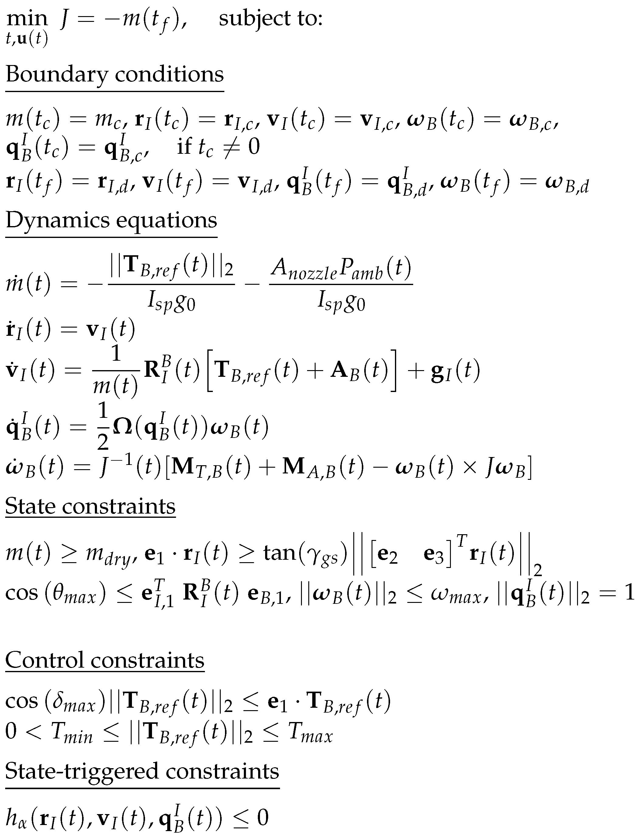
The guidance law relies on solving an optimal control problem with dynamic constraints. These involve the descent dynamics, but it is also possible to add several state and control constraints. The following paragraphs describe the optimisation problem implemented in the successive convex optimisation loop. Note that the superscript i that defines the current iteration loop is omitted from the following description for the sake of clarity. Figure 6 shows the nonconvex optimisation problem defined for this study.

It can be observed that the 6-DoF nonlinear descent dynamics displayed in Equations (4)–(6) are re-adapted to the 6-DoF descent of a powered-only first-stage booster, meaning that only the thrust vector of the main engine, denoted hereafter as ${\mathbf{T}}_{ref,B}\left(t\right)$, is considered as the control input $\mathbf{u}\left(t\right)$. In fact, the steerable planar fins are not included in the optimisation problem for the rocket D&L in order to avoid adding complexity due to the nonlinearities generated by the addition of these aerodynamic loads. This is common practice for launcher re-entry, since the thrust vector (magnitude and direction) is a good indicator for reference trajectory generation. The allocation between the actuators, TVC, and steerable planar fins is achieved afterwards by the control subsystem using the reference values obtained in terms of thrust magnitude and attitude angles.

In addition, the aerodynamics are modelled through a so-called spherical aerodynamic model. This model, introduced by Szmuk et al. in Ref. [4], approximates the relationship between the aerodynamic force and the velocity vector and has the advantage of being easily implementable with the successive convex optimisation guidance method. More specifically, the aerodynamic force ${\mathbf{A}}_B\left(t\right)$ is considered to be always anti-parallel with respect to the velocity ${\mathbf{v}}_B\left(t\right)$ as if the vehicle were subjected to a pure drag force. Assuming that the rocket is axisymmetric, the aerodynamic forces and moments in the vehicle’s body-fixed reference frame are expressed by

$$\begin{array}{cc}\hfill {\mathbf{A}}_B\left(t\right)& =-\frac{1}{2}\rho \left(t\right)\left|\right|{\mathbf{v}}_I\left(t\right){\left|\right|}_2{S}_{ref}{C}_{aero}\left(t\right){\mathbf{R}}_B^I\left(t\right){\mathbf{v}}_I\left(t\right)\hfill \\ \hfill {\mathbf{M}}_{A,B}\left(t\right)& =\left[{\mathbf{x}}_{CP}-{\mathbf{x}}_{CG}\left(t\right)\right]\times {\mathbf{A}}_B\left(t\right)\hfill \end{array}$$

(22)

Here, $C_{aero}\left(t\right)=\mathrm{diag}\left(\left[\begin{array}{ccc}{c}_{a,x}\left(t\right)& c_{a,x}\left(t\right)& c_{a,x}\left(t\right)\end{array}\right]\right)$ is the aerodynamic coefficient matrix, where $c_{a,x}\left(t\right)$ is a positive scalar defined as follows

$$c_{a,x}\left(t\right)=C_D(\alpha =\pi ,M\left(t\right))$$

(23)

Here, $C_D(\alpha \left(t\right),M\left(t\right))$ is the drag coefficient, which is estimated from the available lookup tables defined in Section 2.3.

Regarding the state constraints, the first is a lower bound of the mass: for any time $t\in [t_c,t_f]$, the mass cannot be lower than the dry mass of the vehicle. This constraint is expressed as follows:

$$m\left(t\right)\ge m_{dry}.$$

(24)

The second constraint is the so-called glide-slop constraint: it restricts the inertial position to lie within a glide-slope cone with half-angle ${\gamma }_{gs}\in [0,90\mathrm{deg})$ and a vertex at the landing site. This constraint is enforced by

$${\mathbf{e}}_1·{\mathbf{r}}_I\left(t\right)\ge tan\left({\gamma }_{gs}\right){\left|\left|{\left[\begin{array}{cc}{\mathbf{e}}_2& {\mathbf{e}}_3\end{array}\right]}^T{\mathbf{r}}_I\left(t\right)\right|\right|}_2$$

(25)

where ${\mathbf{e}}_i,i\in [1,3]$ are the versors. The third constraint then concerns the tilt angle, that is, the angle between the $\mathbf{x}$-axes of the two reference frames, which is limited to a maximum of ${\theta }_{max}\in (0,90\mathrm{deg}]$. It is defined by

$$cos\left({\theta }_{max}\right)\le {\mathbf{e}}_{I,1}^T{\mathbf{R}}_I^B\left(t\right){\mathbf{e}}_{B,1}.$$

(26)

Then, the fourth constraint limits the angular rate of the vehicle and is enforced by

$$\left|\right|{\mathit{\omega }}_B\left(t\right){\left|\right|}_2\le {\omega }_{max}.$$

(27)

Finally, an additional constraint preserves the unit norm of the quaternion as follows:

$$\left|\right|{\mathbf{q}}_B^I\left(t\right){\left|\right|}_2=1.$$

(28)

Moreover, a so-called State-Triggered Constraint (STC) [4] is added. In the present case, it consists in imposing an angle of attack $\alpha$ constraint, ${\alpha }_{max}$, when the dynamic pressure $Q\left(t\right)$ is larger than a prescribed value $Q_{max}$. This constraint is written in a continuous formulation with a trigger function $g_{\alpha }$ and a constraint function $c_{\alpha }$ as follows:

$$\begin{array}{cc}\hfill h_{\alpha }({\mathbf{r}}_I\left(t\right),{\mathbf{v}}_I\left(t\right),{\mathbf{q}}_B^I\left(t\right))& =-min(g_{\alpha }({\mathbf{v}}_I\left(t\right),{\mathbf{r}}_I\left(t\right)),0)·c_{\alpha }\le 0\hfill \\ \hfill c_{\alpha }({\mathbf{v}}_I\left(t\right),{\mathbf{q}}_B^I\left(t\right))& ={\mathbf{e}}_1·{\mathbf{R}}_B^I\left(t\right){\mathbf{v}}_I\left(t\right)+cos\left({\alpha }_{max}\right)\left|\right|{\mathbf{v}}_I\left(t\right){\left|\right|}_2\hfill \\ \hfill g_{\alpha }({\mathbf{r}}_I\left(t\right),{\mathbf{v}}_I\left(t\right))& =Q_{max}-\frac{1}{2}\rho \left(t\right)\left|\right|{\mathbf{v}}_I\left(t\right){\left|\right|}_2^2.\hfill \end{array}$$

(29)

Two control constraints are considered to bound the direction and magnitude of the thrust force. The direction is bounded by limiting the TVC up to a maximum gimbal angle ${\delta }_{max}$. It is enforced by

$$cos\left({\delta }_{max}\right)\left|\right|{\mathbf{T}}_{B,ref}\left(t\right){\left|\right|}_2\le {\mathbf{e}}_1·{\mathbf{T}}_{B,ref}\left(t\right).$$

(30)

Then, the thrust magnitude is bounded between minimum and maximum values, i.e.,

$$0<T_{min}\le \left|\right|{\mathbf{T}}_{B,ref}\left(t\right){\left|\right|}_2\le T_{max}$$

(31)

where $T_{min}$ and $T_{max}$ are the lower and upper bounds, respectively.

The objective of the optimal control problem defined herein is to find the optimal trajectory subject to the defined re-entry dynamics and state and control constraints while minimising the vehicle’s fuel consumption, which corresponds to maximising the vehicle’s final mass. Therefore, the cost function can be written as follows at each ith SOCP iteration:

$$J=-m\left(t_f\right).$$

(32)

3.2. SOCP Problem

However, the optimisation problem subject to the described dynamics and state and control constraints is not convex and must therefore be convexified. In order to achieve this, the first step is to convert the free-final-time nonlinear continuous-time optimal control problem into an equivalent fixed-final-time nonlinear continuous-time problem. This is achieved by normalising the time of flight from $t\in [t_c,t_f]$ to $\tau \in [0,1]$, where $\tau$ is the normalised time of flight. The nonlinear dynamics are summarised as $\dot{\mathbf{x}}\left(t\right)=f(\mathbf{x}\left(t\right),\mathbf{u}\left(t\right))$ with $\mathbf{x}\left(t\right)={\left[\begin{array}{ccccc}m\left(t\right)& {\mathbf{r}}_I^T\left(t\right)& {\mathbf{v}}_I^T\left(t\right)& {\mathbf{q}}_B^I{\left(t\right)}^T& {\mathit{\omega }}_B^T\left(t\right)\end{array}\right]}^T$ as the state vector and $\mathbf{u}\left(t\right)={\mathbf{T}}_{B,ref}\left(t\right)$ as the control vector, which can be rewritten as follows:

$$\dot{\mathbf{x}}\left(t\right)=\frac{\mathrm{d}\tau }{\mathrm{d}t}\frac{\mathrm{d}}{\mathrm{d}\tau }\mathbf{x}\left(t\right).$$

(33)

Therefore, with $\sigma ={\left(\mathrm{d}\tau /\mathrm{d}t\right)}^{-1}$, the normalised nonlinear dynamics are expressed by

$$\frac{\mathrm{d}}{\mathrm{d}\tau }\mathbf{x}\left(\tau \right)=\sigma ·f(\mathbf{x}\left(\tau \right),\mathbf{u}\left(\tau \right))$$

(34)

where $\sigma =t_f$, since $\tau \in [0,1]$.

Then, the nonlinear descent dynamics equations, defined above, are linearised and discretised about the solution of the previous iteration through a first-order Taylor approximation and using a zero-order-hold interpolation scheme. First, the original continuous-time problem is transformed into a Linear Time-Varying (LTV) problem defined by

$$\frac{\mathrm{d}}{\mathrm{d}\tau }\mathbf{x}\left(\tau \right)=\mathbf{A}\left(\tau \right)\mathbf{x}\left(\tau \right)+\mathbf{B}\left(\tau \right)\mathbf{u}\left(\tau \right)+\mathbf{\Sigma }\left(\tau \right)\sigma +\mathbf{z}\left(\tau \right)$$

(35)

where the parameters are evaluated about a reference trajectory corresponding to the previous ($i-1$)th SOCP solution:

$$\begin{array}{cc}\hfill \mathbf{A}\left(\tau \right)& :={\sigma }^{i-1}·\frac{\partial f}{\partial \mathbf{x}}{|}_{{\mathbf{x}}^{i-1}\left(\tau \right),{\mathbf{u}}^{i-1}\left(\tau \right)}\hfill \\ \hfill \mathbf{B}\left(\tau \right)& :={\sigma }^{i-1}·\frac{\partial f}{\partial \mathbf{u}}{|}_{{\mathbf{x}}^{i-1}\left(\tau \right),{\mathbf{u}}^{i-1}\left(\tau \right)}\hfill \\ \hfill \mathbf{\Sigma }\left(\tau \right)& :=f({\mathbf{x}}^{i-1}\left(\tau \right),{\mathbf{u}}^{i-1}\left(\tau \right))\hfill \\ \hfill \mathbf{z}\left(\tau \right)& :=-\mathbf{A}\left(\tau \right){\mathbf{x}}^{i-1}\left(\tau \right)-\mathbf{B}\left(\tau \right){\mathbf{u}}^{i-1}\left(\tau \right).\hfill \end{array}$$

(36)

Second, the discretised LTV system is given for each $k\in [1,K-1]$ by

$$\begin{array}{cc}\hfill \mathbf{x}[k+1]& =\overline{\mathbf{A}}\left[k\right]\mathbf{x}\left[k\right]+\overline{\mathbf{B}}\left[k\right]\mathbf{u}\left[k\right]+\overline{\mathbf{\Sigma }}\left[k\right]\sigma +\overline{\mathbf{z}}\left[k\right],\hfill \\ \hfill \overline{\mathbf{A}}\left[k\right]& :={\mathbf{I}}_{n_x\times n_x}+{\mathrm{T}}_s\mathbf{A}\left[k\right],\hfill \\ \hfill \overline{\mathbf{B}}\left[k\right]& :={\mathrm{T}}_s\mathbf{B}\left[k\right],\hfill \\ \hfill \overline{\mathbf{\Sigma }}\left[k\right]& :={\mathrm{T}}_s\mathbf{\Sigma }\left[k\right],\hfill \\ \hfill \overline{\mathbf{z}}\left[k\right]& :={\mathrm{T}}_s\mathbf{z}\left[k\right].\hfill \end{array}$$

(37)

Once the descent dynamics are linearised and discretised, the next step is the convexification of the nonconvex constraints. This concerns two state constraints, the norm of the quaternion (Equation (28)) and the STC (Equation (29)), and one control constraint, the lower bound of the thrust magnitude (Equation (31)). The convexification of Equation (28) is obtained through a first-order Taylor expansion approximation evaluated about the previous $(i-1)$th SOCP iteration:

$$\left|\right|{\mathbf{q}}_B^{I,i-1}\left[k\right]{\left|\right|}_2+\frac{{\mathbf{q}}_B^{I,i-1}{\left[k\right]}^T}{\left|\right|{\mathbf{q}}_B^{I,i-1}\left[k\right]{\left|\right|}_2}({\mathbf{q}}_B^{I,i}\left[k\right]-{\mathbf{q}}_B^{I,i-1}\left[k\right])=1.$$

(38)

The same method is used for the STC (Equation (29)). However, due to the $min(·)$ function, the constraint is approximated as follows:

$$\left\{\begin{array}{cc}\hfill h_{\alpha }\left({\mathit{\xi }}^{i-1}\left[k\right]\right)+{\left.\frac{\partial h_{\alpha }}{\partial \mathit{\xi }}\right|}_{{\mathit{\xi }}^{i-1}\left[k\right]}({\mathit{\xi }}^i\left[k\right]-{\mathit{\xi }}^{i-1}\left[k\right])\le 0,& \mathrm{if}{g}_{\alpha }\left({\mathit{\xi }}^{i-1}\left[k\right]\right)<0\hfill \\ \hfill 0,& \mathrm{otherwise}\hfill \end{array}\right.$$

(39)

where ${\mathit{\xi }}^i\left[k\right]={\left[\begin{array}{cc}{\mathbf{v}}_I^i{\left[k\right]}^T& {\mathbf{q}}_B^{I,i}{\left[k\right]}^T\end{array}\right]}^T,\forall k\in [1,K]$ are the reference trajectory parameters obtained from the ith SOCP iteration. Lastly, it is applied to the lower bound of the thrust magnitude, obtaining the following expression for $k\in [1,K-1]$:

$$\begin{array}{cc}\hfill & h_T\left(\mathbf{u}\left[k\right]\right)=T_{min}-\left|\right|{\mathbf{T}}_{B,ref}\left[k\right]{\left|\right|}_2\hfill \\ \hfill & h_T\left({\mathbf{u}}^{i-1}\left[k\right]\right)+{\left.\frac{\partial h_T}{\partial \mathbf{u}}\right|}_{{\mathbf{u}}^{i-1}\left[k\right]}({\mathbf{u}}^i\left[k\right]-{\mathbf{u}}^{i-1}\left[k\right])\le 0.\hfill \end{array}$$

(40)

The successive convex optimisation strategy involves the use of trust regions and virtual controls to prevent unboundedness and artificial infeasibility, respectively. In fact, these issues are due to the linearisation process. They could be avoided using the nonlinearity preservation and linearisation approach instead of the direct linearisation approach adopted in this guidance law to reduce complexity [29,30]. The implementation of trust regions allows one to limit the deviation between two consecutive iterations responsible for artificial unboundedness. They consist of quadratic inequality constraints. The aim is to define a region near the previous iteration so that the deviation is mitigated. As a consequence, this involves the radius being penalised in the cost function. In this optimisation problem, the trust regions are defined first for the state and control vectors and then for the time of flight as follows:

$$\begin{array}{cc}\hfill \left|\right|{\mathbf{x}}^i\left[k\right]-{\mathbf{x}}^{i-1}{\left[k\right]\left|\right|}_2+\left|\right|{\mathbf{u}}^i\left[k\right]-{\mathbf{u}}^{i-1}\left[k\right]{\left|\right|}_2& \le {\Delta }_{\mathbf{x},\mathbf{u}}^i\left[k\right]\hfill \\ \hfill \left|\right|{\sigma }^i-{\sigma }^{i-1}{\left|\right|}_2& \le {\Delta }_{\sigma }^i.\hfill \end{array}$$

(41)

${\mathbf{\Delta }}_{\mathbf{x},\mathbf{u}}^i={\left[\begin{array}{ccc}{\Delta }_{\mathbf{x},\mathbf{u}}^i\left[1\right],& \cdots ,& {\Delta }_{\mathbf{x},\mathbf{u}}^i\left[K\right]\end{array}\right]}^T\in {\mathbb{R}}^K$ is then defined as the state and control trust region vector. To convert this trust region vector into the SOCP formulation, it is necessary to define a joint state and control vector at each time instant, ${\mathit{\xi }}^i\left[k\right]={\left[\begin{array}{cc}{\left({\mathbf{x}}^i\left[k\right]\right)}^T& {\left({\mathbf{u}}^i\left[k\right]\right)}^T\end{array}\right]}^T$, $k\in [1,K-1]$ so that Equation (41) can be rewritten as

$$\left|\right|\begin{array}{cc}\hfill (1-2{\left({\mathit{\xi }}^{i-1}\left[k\right]\right)}^T{\mathit{\xi }}^i\left[k\right]+& ({\left({\mathit{\xi }}^{i-1}\left[k\right]\right)}^T{\mathit{\xi }}^{i-1}\left[k\right]-{\Delta }_{\mathbf{x},\mathbf{u}}^i\left[k\right]))/2\hfill \\ & {\mathbf{I}}_{n_{\xi }\times n_{\xi }}{\mathit{\xi }}^i\left[k\right]\hfill \end{array}|{|}_2\le (1+2{\left({\mathit{\xi }}^{i-1}\left[k\right]\right)}^T{\mathit{\xi }}^i\left[k\right]-({\left({\mathit{\xi }}^{i-1}\left[k\right]\right)}^T{\mathit{\xi }}^{i-1}\left[k\right]-{\Delta }_{\mathbf{x},\mathbf{u}}^i\left[k\right]))/2.$$

(42)

Finally, the size of the trust regions must be bounded; therefore, the norms ${\mathbf{\Delta }}_{\mathbf{x},\mathbf{u}}^i$ and ${\mathbf{\Delta }}_{\sigma }^i$ must be inserted into the cost function. Regarding the state and control trust region vector, a slack variable $S_{{\mathbf{\Delta }}_{\mathbf{x},\mathbf{u}}}^i$ must be introduced in order to avoid a quadratic term in the cost function. This implies the addition of the following inequality constraint [26]:

$$\left|\right|{\mathbf{\Delta }}_{\mathbf{x},\mathbf{u}}^i{\left|\right|}_2\le S_{{\mathbf{\Delta }}_{\mathbf{x},\mathbf{u}}}^i.$$

(43)

Virtual controls are additional control inputs ${\mathit{\nu }}^i\in {\mathbb{R}}^{n_x}$ that allow one to reach each point of the solution domain through dynamics relaxation and therefore avoid artificial infeasibility. They are commonly met during the first iterations of the algorithm due to the dynamically inconsistent initial guess, but they also compensate for the high-order terms neglected by the discretisation process. Therefore, the linear discrete dynamics of Equation (37) become

$${\mathbf{x}}^i[k+1]=\overline{\mathbf{A}}\left[k\right]{\mathbf{x}}^i\left[k\right]+\overline{\mathbf{B}}\left[k\right]{\mathbf{u}}^i\left[k\right]+\overline{\mathbf{\Sigma }}\left[k\right]\sigma +{\overline{\mathbf{z}}}^i\left[k\right]+{\mathit{\nu }}^i\left[k\right].$$

(44)

We can then define a concatenated vector ${\overline{\mathit{\nu }}}^i:={\left[\begin{array}{ccc}{\left({\mathit{\nu }}^i\left[1\right]\right)}^T,& \cdots ,& {\left({\mathit{\nu }}^i[K-1]\right)}^T\end{array}\right]}^T\in {\mathbb{R}}^{n_x\times (K-1)}$. Similarly to the trust regions, all these terms must be penalised in the cost function, and to avoid a quadratic term, a slack variable $S_{\mathit{\nu }}^i$ must be again be defined in conjunction with the following inequality constraint:

$$\begin{array}{c}\hfill \left|\right|{\overline{\mathit{\nu }}}^i{\left|\right|}_2\le S_{\mathit{\nu }}^i.\end{array}$$

(45)

Finally, the cost function of Equation (32) is augmented with the previously defined features and becomes:

$$J=-m^i\left[K\right]+w_{\mathit{\nu }}{S}_{\mathit{\nu }}^i+w_{{\mathbf{\Delta }}_{\mathbf{x},\mathbf{u}}}{S}_{{\mathbf{\Delta }}_{\mathbf{x},\mathbf{u}}}^i+w_{{\Delta }_{\sigma }}{\Delta }_{\sigma }^i$$

(46)

where $w_{\mathit{\nu }}$, $w_{{\mathbf{\Delta }}_{\mathbf{x},\mathbf{u}}}$, and $w_{{\Delta }_{\sigma }}$ are penalisation weights.

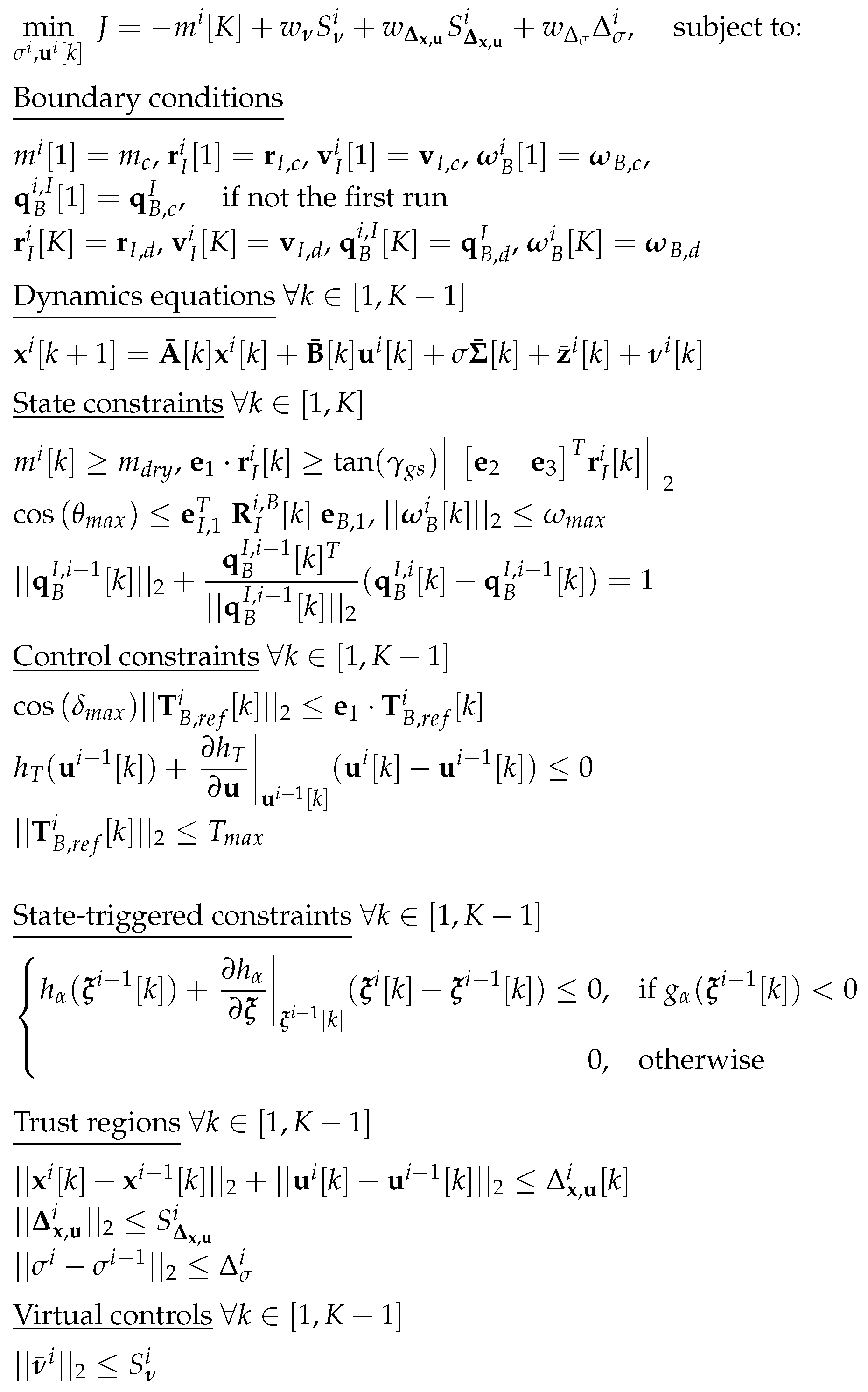
The obtained SOCP optimisation problem, which is solved iteratively in the successive convex optimisation algorithm, is summarised in Figure 7.

Table 3. SOCP optimisation problem parameters.

Parameter	Value	Units	Parameter	Value	Units
${\omega }_{\Delta }$	1	-	$T_{max}$	600	kN
${\omega }_{\nu }$	1000	-	$T_{min}$	0	kN
${\omega }_{\sigma }$	0.75	-	${\omega }_{max}$	28.6	deg/s
$i_{max}$	10	-	${\theta }_{max}$	75	deg
${\Delta }_{tol}$	0.001	-	${\gamma }_{gs}$	10	deg
K	100	-	${\delta }_{max}$	10	deg
$t_f^0$	120	s	${\alpha }_{max}$	5	deg
$m_{dry}$	2750	kg	$Q_{max}$	$4\times {10}^4$	Pa

provides the SOCP problem parameters.

4. Control Approach

From the reference trajectory computed by the previously defined guidance algorithm and the current states of the vehicle, the control algorithm must be able to generate the necessary commands in terms of the thrust magnitude $T_{ref}\left(t\right)$; TVC deflection angles $\{{\beta }_{TVC,y}\left(t\right),{\beta }_{TVC,z}\left(t\right)\}$; and fin deflections $\{{\beta }_{fin,1}\left(t\right),{\beta }_{fin,2}\left(t\right),{\beta }_{fin,3}\left(t\right),{\beta }_{fin,4}\left(t\right)\}$ to be applied by the actuators in order to correct the trajectory of the vehicle. For this study, we assume ${\beta }_{fin,1}\left(t\right)={\beta }_{fin,2}\left(t\right)={\beta }_{fin,y}\left(t\right)$ and ${\beta }_{fin,3}\left(t\right)={\beta }_{fin,4}\left(t\right)={\beta }_{fin,z}\left(t\right)$. The method adopted here considers the use of two gain-scheduled PID controllers to compute the respective deflection angles. In fact, the thrust magnitude command is taken directly from the guidance algorithm $T_{ref}\left(t\right)=\left|\right|{\mathbf{T}}_{B,ref}\left(t\right){\left|\right|}_2$. This approximation is penalised by a low-pass filter, which simulates the intrinsic physics of the device, and the delay induced is compensated for by a PI controller. In fact, the descent control system is more complex than the ascent phase due to the throttleability of the thrust force generated by the rocket’s main engine. If this were considered as a control input, the pitch and yaw motion could not be decoupled, as is usually carried out for rocket preliminary attitude control design. We followed this approach herein since the objective was primarily to study the interactions between all the subsystems, rather than the development of a highly accurate, high-performance control system.

Usually, the 6-DoF problem is separated into two 3-DoF problems. One is characterised by the motion in the ${\mathbf{x}}_{\mathit{B}}{\mathbf{z}}_{\mathit{B}}$ plane with the controller on the pitch angle $\theta \left(t\right)$ through the deflection angles ${\beta }_{TVC,y}\left(t\right)$ and ${\beta }_{fin,y}\left(t\right)$. The second problem is characterised by the motion in the ${\mathbf{x}}_{\mathit{B}}{\mathbf{y}}_{\mathit{B}}$ plane with the controller on the yaw angle $\psi \left(t\right)$ through the deflection angles ${\beta }_{TVC,z}\left(t\right)$ and ${\beta }_{fin,z}\left(t\right)$. An assumption is made that the roll angle $\varphi \left(t\right)$ is small so that no coupling effects can arise in the dynamics. Therefore, two linear systems are built using a reference trajectory precomputed offline. This reference trajectory corresponds to the solution of the successive convex optimisation algorithm in its first run, meaning that the initial conditions of the studied problem are used. These can be rewritten in terms of the perturbed variables $\tilde{\mathbf{x}}\left(t\right)=\mathbf{x}\left(t\right)-\overline{\mathbf{x}}\left(t\right)$ and $\tilde{\mathbf{u}}\left(t\right)=\mathbf{u}\left(t\right)-\overline{\mathbf{u}}\left(t\right)$, where $\overline{\mathbf{x}}\left(t\right)$ and $\overline{\mathbf{u}}\left(t\right)$ are the reference state and control vectors, respectively, to finally obtain

$$\begin{array}{cc}\hfill & \dot{\tilde{\mathbf{x}}}\left(t\right)=\mathbf{A}\left(t\right)\tilde{\mathbf{x}}\left(t\right)+\mathbf{B}\left(t\right)\tilde{\mathbf{u}}\left(t\right)\hfill \\ \hfill & \mathbf{y}\left(t\right)=\mathbf{C}\left(t\right)\tilde{\mathbf{x}}\left(t\right)\hfill \end{array}$$

(47)

where $\mathbf{A}\left(t\right)\in {\mathbb{R}}^{10\times 10}$ and $\mathbf{B}\left(t\right)\in {\mathbb{R}}^{10\times 4}$ are the Jacobian matrices of the nonlinear equations with respect to the state and control variables respectively, computed with the function $\mathtt{jacobian}$ in MATLAB, and $\mathbf{C}\left(t\right)\in {\mathbb{R}}^{2\times 10}$ enables the extraction of the pitch angle error $\tilde{\theta }\left(t\right)$ and the yaw angle error $\tilde{\psi }\left(t\right)$. Therefore, the decoupling into two 3-DoF is achieved, and the following linear systems are obtained:

$$\begin{array}{cc}\hfill {\mathbf{x}}_{pitch}\left(t\right)& ={\left[\begin{array}{ccccc}m\left(t\right)& v_x\left(t\right)& v_z\left(t\right)& {\omega }_y\left(t\right)& \theta \left(t\right)\end{array}\right]}^T\in {\mathbb{R}}^5,\hfill \\ \hfill {\mathbf{u}}_{pitch}\left(t\right)& ={\left[\begin{array}{cc}{\beta }_{TVC,y}\left(t\right)& {\beta }_{fin,y}\left(t\right)\end{array}\right]}^T\in {\mathbb{R}}^2,{\mathbf{y}}_{pitch}\left(t\right)=\theta \left(t\right)\in \mathbb{R}\hfill \\ \hfill {\mathbf{x}}_{yaw}\left(t\right)& ={\left[\begin{array}{ccccc}m\left(t\right)& v_x\left(t\right)& v_y\left(t\right)& {\omega }_z\left(t\right)& \psi \left(t\right)\end{array}\right]}^T\in {\mathbb{R}}^5,\hfill \\ \hfill {\mathbf{u}}_{yaw}\left(t\right)& ={\left[\begin{array}{cc}{\beta }_{TVC,y}\left(t\right)& {\beta }_{fin,y}\left(t\right)\end{array}\right]}^T\in {\mathbb{R}}^2,{\mathbf{y}}_{yaw}\left(t\right)=\psi \left(t\right)\in \mathbb{R}\hfill \end{array}$$

(48)

where $v_x\left(t\right)$, $v_y\left(t\right)$, and $v_z\left(t\right)$ are the x, y, and z components of ${\mathbf{v}}_B\left(t\right)$, respectively, and ${\omega }_y\left(t\right)$ and ${\omega }_z\left(t\right)$ are the y and z components of ${\mathit{\omega }}_B\left(t\right)$. The corresponding Jacobian matrices are computed similarly to the linear system defined in Equation (47). This decoupling of the dynamics was validated in [26].

With these definitions and because two control inputs are considered in each linear system (TVC and fin deflections), the latter is considered as a Multiple-Input Multiple-Output (MIMO) control system for which it is complex to apply classical linear control theory since every channel must be iteratively addressed in a single-loop fashion. The solution to overcome this drawback would be the use of advanced robust control methods such as the $H_{\infty }$ family of methods or the LPV approach. A preliminary study of structured $H_{\infty }$ control synthesis within this simulator is available in Ref. [31]. In this study, to develop a baseline simulator and stay in line with the current state of the art in control design for launchers [10,32], the linear systems are adapted to Single-Input Single-Output (SISO) control systems, for which it is possible to use gain-scheduled PID controllers. Two configurations are chosen and are explained in the next subsections. The first is the TVC-only configuration, for which the fins are considered fixed and the only input is therefore the TVC deflection. The second configuration lies in the definition of a control moment, introduced in Ref. [16], which gathers TVC and fin control authorities and then allocates the necessary command to each actuator according to the level of thrust.

4.1. TVC-Only SISO Configuration

In this case, the only control inputs are ${\beta }_{TVC,y}\left(t\right)$ for the pitch plane and ${\beta }_{TVC,z}\left(t\right)$ for the yaw plane. Therefore, the two linear systems consider the following parameters:

$$\begin{array}{cc}\hfill {\mathbf{x}}_{pitch}\left(t\right)& ={\left[\begin{array}{ccccc}m\left(t\right)& v_x\left(t\right)& v_z\left(t\right)& {\omega }_y\left(t\right)& \theta \left(t\right)\end{array}\right]}^T\in {\mathbb{R}}^5,\hfill \\ \hfill {\mathbf{u}}_{pitch}\left(t\right)& ={\beta }_{TVC,y}\left(t\right),{\mathbf{y}}_{pitch}\left(t\right)=\theta \left(t\right)\hfill \\ \hfill {\mathbf{x}}_{yaw}\left(t\right)& ={\left[\begin{array}{ccccc}m\left(t\right)& v_x\left(t\right)& v_y\left(t\right)& {\omega }_z\left(t\right)& \psi \left(t\right)\end{array}\right]}^T\in {\mathbb{R}}^5,\hfill \\ \hfill {\mathbf{u}}_{yaw}\left(t\right)& ={\beta }_{TVC,z}\left(t\right),{\mathbf{y}}_{yaw}\left(t\right)=\psi \left(t\right)\hfill \end{array}$$

(49)

where $v_x\left(t\right)$, $v_y\left(t\right)$, and $v_z\left(t\right)$ are the x, y, and z components of ${\mathbf{v}}_B\left(t\right)$, respectively, and ${\omega }_y\left(t\right)$ and ${\omega }_z\left(t\right)$ are the y and z components of ${\mathit{\omega }}_B\left(t\right)$. The corresponding Jacobian matrices are computed similarly to the linear system defined in Equation (47).

Due to the time-varying nature of the problem, a single PID controller might be unable to stabilise the system for the whole trajectory. Therefore, the reference altitude profile is discretised into 25 slots where linearisation is performed. This was chosen as the scheduling parameter since it evolves monotonically with respect to time and has been well validated in the literature [33,34]. Moreover, it allows one to capture the variations in terms of thrust magnitude. In this way, the problem is divided into regions wherein it is possible to analyse if the controller is able to stabilise the system. Thanks to this, the controllers can be considered gain-scheduled PID controllers, as the gains can be changed to achieve the desired levels of performance in all the regions. For each system, the gains are tuned with the following performance requirements: an overshoot inferior to 10%, a settling time strictly inferior to 1 s, a gain margin superior to 6 dB, and a phase margin superior to 60 deg. The tuning is performed with the MATLAB application $\mathtt{PID} \mathtt{tuner}$.

4.2. TVC and Fin SISO Configuration

Here, the MIMO formulation is translated into an SISO formulation by defining a surrogate variable that gathers gimbal and fin angle deflections and achieving control synthesis on it. More specifically, following Ref. [16], the control moment $m_{ctr}\left(t\right)$ is defined as a parameter that specifies the necessary pitch or yaw moment to correct the trajectory of the vehicle. Knowing the control effectiveness level of each actuator, a control allocation algorithm is then used to determine the actual control inputs $\{{\beta }_{TVC,y}\left(t\right)$, ${\beta }_{fin,y}\left(t\right)\}$ and $\{{\beta }_{TVC,z}\left(t\right)$, ${\beta }_{fin,z}\left(t\right)\}$.

The control effectiveness levels are expressed as follows. The effectiveness of TVC in generating control moments is quantified by

$${\mu }_{TVC}\left(t\right)=[x_{CG}\left(t\right)-x_{PVP}]\frac{T_{ref}\left(t\right)}{J_N\left(t\right)}.$$

(50)

Regarding the fins, the control effectiveness is given by

$${\mu }_{fin}\left(t\right)=2[x_{fin}-x_{CG}\left(t\right)]\frac{Q\left(t\right)S_{fin}{C}_{N,fin\setminus \alpha }\left(t\right)}{J_N\left(t\right)}$$

(51)

where $C_{N,fin\setminus \alpha }\left(t\right)=2\pi \left(\frac{A{R}_{fin}}{A{R}_{fin}+2}\right)cos\left({\gamma }_{fin,i}\left(t\right)\right)$ is the normal fin force gradient with ${\gamma }_{fin,i}\left(t\right)$ computed from Equation (37) for the pitch plane and Equation (38) for the yaw plane. The relationship between the control moment and the control inputs is then expressed as

$$m_{ctr,\#}\left(t\right)=-{\mu }_{TVC}\left(t\right){\beta }_{TVC,\#}\left(t\right)-{\mu }_{fin}\left(t\right){\beta }_{fin,\#}\left(t\right)$$

(52)

where $\#=\{y,z\}$ for the pitch plane and the yaw plane, respectively.

Therefore, these parameters are obtained from the reference trajectory, and similarly to Equation (47), the following linear systems are built for the pitch and the yaw planes:

$$\begin{array}{cc}\hfill {\mathbf{x}}_{pitch}\left(t\right)& ={\left[\begin{array}{ccccc}m\left(t\right)& v_x\left(t\right)& v_z\left(t\right)& {\omega }_y\left(t\right)& \theta \left(t\right)\end{array}\right]}^T\in {\mathbb{R}}^5,\hfill \\ \hfill {\mathbf{u}}_{pitch}\left(t\right)& =m_{ctr,y}\left(t\right),{\mathbf{y}}_{pitch}\left(t\right)=\theta \left(t\right)\hfill \\ \hfill {\mathbf{x}}_{yaw}\left(t\right)& ={\left[\begin{array}{ccccc}m\left(t\right)& v_x\left(t\right)& v_y\left(t\right)& {\omega }_z\left(t\right)& \psi \left(t\right)\end{array}\right]}^T\in {\mathbb{R}}^5,\hfill \\ \hfill {\mathbf{u}}_{yaw}\left(t\right)& =m_{ctr,z}\left(t\right),{\mathbf{y}}_{yaw}\left(t\right)=\psi \left(t\right).\hfill \end{array}$$

(53)

The Jacobian matrices and the corresponding PIDs for the given altitude slots are computed in the same manner as for the previous configuration. Note that the obtained controllers must be robust enough to cope with a range of trajectories since the guidance is recomputed several times during the descent, but not the tuning of the gains. However, it is observed that the updated guidance trajectories follow the same scheme, which is enforced by the boundary constraint on the quaternion (recall Figure 7), and since the controllers are interpolated with respect to the altitude (and not the time of flight, which is unknown), the obtained gains provide satisfactory results all along the descent flight.

Finally, the commanded control moment $m_{ctr}\left(t\right)$ is allocated between the TVC system and the planar fins following the algorithm in Ref. [16], repeated in Algorithm 1. More specifically, if the commanded thrust magnitude $T_{ref}\left(t\right)$ is above the user-defined high thrust limit $T_{HTL}$, then the TVC system is used as the primary actuator, and the planar fins are used only if the maximum authority ${\beta }_{TVC,max}$ of the TVC system is reached. In contrast, if the thrust magnitude command $T_{ref}\left(t\right)$ is below the user-defined high thrust limit $T_{HTL}$, then the planar fins are used as the primary actuator, and the TVC system is used as the secondary actuator if the maximum authority ${\beta }_{fin,max}$ of the planar fins is reached. Here, ${\beta }_{TVC,max}=10\mathrm{deg}$ and ${\beta }_{fin,max}=20\mathrm{deg}$.

Algorithm 1 Control allocation [16]

1: if  $T_{ref}\ge T_{HTL}$  then   2:       ${\beta }_{TVC}\leftarrow -m_{ctr}/{\mu }_{TVC}$   3:       ${\beta }_{fin}\leftarrow 0$   4:       if $|{\beta }_{TVC}|>{\beta }_{TVC,max}$ then   5:            ${\beta }_{TVC}\leftarrow {\beta }_{TVC,max}\times sign\left({\beta }_{TVC}\right)$   6:            ${\beta }_{fin}\leftarrow -(m_{ctr}+{\mu }_{TVC}\times {\beta }_{TVC})/{\mu }_{fin}$   7:       end if   8: else   9:       ${\beta }_{fin}\leftarrow -m_{ctr}/{\mu }_{fin}$ 10:       ${\beta }_{TVC}\leftarrow 0$ 11:       if $|{\beta }_{fin}|>{\beta }_{fin,max}$ then 12:            ${\beta }_{fin}\leftarrow {\beta }_{fin,max}\times sign\left({\beta }_{fin}\right)$ 13:            ${\beta }_{TVC}\leftarrow -(m_{ctr}+{\mu }_{fin}\times {\beta }_{fin})/{\mu }_{TVC}$ 14:       end if 15: end if 16: OUTPUTS: ${\beta }_{TVC}$, ${\beta }_{fin}$

Note that this control configuration also enables a fin-only actuation configuration by setting a high thrust limit $T_{HTL}$ superior to the maximum thrust magnitude allowed by the guidance algorithm. Note also that this choice of criteria for changing the actuator allocation configuration was made after further analyses. Other criteria were tested, such as dynamic pressure or control effectiveness levels, that is, allocation primarily to the TVC system if ${\mu }_{TVC}\left(t\right)>{\mu }_{fin}\left(t\right)$ and to the planar fins otherwise. However, the dynamic pressure profile was not accurate enough, since at the beginning of the trajectory the dynamic pressure is high, as well as the thrust magnitude; thus, the planar fins are efficient but in reality not as efficient as the TVC system. Furthermore, the control effectiveness level was not optimal, since some overlaps when both actuators had a similar control authority were observed that could lead to convergence issues, since it would involve rapid switches in the commands given to the actuators. Moreover, since the reference thrust magnitude is among the control inputs and completely decoupled from the TVC system by design, this parameter is less complex to implement, preventing coupling effects and therefore leading to the best results.

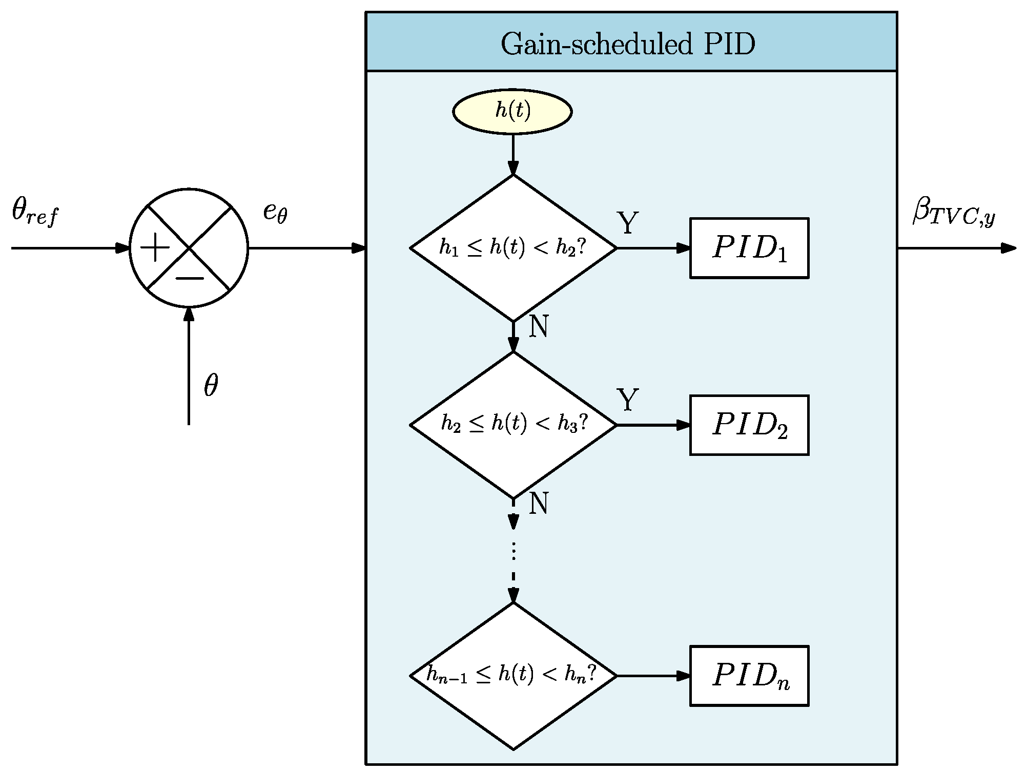
Once verified through linear analysis, the controllers were implemented in the nonlinear simulator according to the actual altitude following the scheme described in Figure 8. Basically, no interpolation was achieved, and a controller was selected as soon as we entered the altitude region in which this controller had been defined. Note that the controllers’ gains could have been interpolated linearly with respect to the altitude using a finite-difference method as in Ref. [33]. However, this solution was not adopted, since the values of two adjacent gain-scheduled controllers were considerably different, leading to inaccuracies when achieving the interpolation. Another strategy would be to use a so-called signal blending scheme to mitigate the previous issue [34]. However, this could cause large transients in the switching regions and would be quite complex to implement. Therefore, this technique was not studied, since the objective was primarily the design of a closed-loop baseline simulator. The gain-scheduling method should be more thoroughly investigated in future work, since an improved scheduling strategy would be a substantial extension for enhanced robustness.

5. Simulation Results

This section illustrates the results obtained with the proposed G&C architecture coupled with the RLV controlled dynamics simulator under different control configurations: TVC-only, fins-only, and both (Section 5.1). Then, a sensitivity analysis is carried out to assess the impact on the obtained trajectory from disturbances such as wind gusts as well as multiple uncertainties through a Monte Carlo approach (Section 5.2).

5.1. Nominal Trajectory Simulations for Different Actuation Configurations

For this study, no wind was considered, and neither propellant sloshing effects nor flexible bending modes were included, since the described simulator is still at an early design stage and more complex studies are necessary for future developments. Three different actuation configurations were tested. The first one with TVC actuation only used the control architecture defined in Section 4.1 and considered fixed planar fins with 0 deg deflection. The second used only planar fins actuation with the control architecture defined in Section 4.2 (with $T_{HTL}=T_{max}=600\mathrm{kN}$). Finally, the third configuration used TVC and planar fins actuation with a thrust magnitude limit of $T_{HTL}=70\mathrm{kN}$. The initial and final conditions are described in

Table 4. Initial and final conditions.

Parameter	Value	Parameter	Value
${\mathbf{r}}_I\left[0\right]$	${[250-15]}^T$$\mathrm{km}$	${\mathbf{r}}_I\left[K\right]$	${\left[000\right]}^T$$\mathrm{m}$
${\mathbf{v}}_I\left[0\right]$	${[-8500950]}^T$$\mathrm{m}/\mathrm{s}$	${\mathbf{v}}_I\left[K\right]$	${[-500]}^T$$\mathrm{m}/\mathrm{s}$
${\mathit{\omega }}_B\left[0\right]$	${\left[000\right]}^T$$\mathrm{rad}/\mathrm{s}$	${\mathit{\omega }}_B\left[K\right]$	${\left[000\right]}^T$$\mathrm{rad}/\mathrm{s}$
$m\left[0\right]$	$\mathrm{14,000}$  $\mathrm{kg}$	${\mathbf{q}}_B^I\left[K\right]$	${\left[0001\right]}^T$

. The initial conditions allowed us to study a trajectory evolving mainly in the pitch plane. Other simulations were also carried out for a trajectory mainly in the yaw plane and for a trajectory in both planes, showing similar results; therefore, they are not displayed in this paper.

Figure 9 shows the converged trajectories for the different cases, as well as the control contributions of the vehicle through the TVC and fin deflection angles and the thrust magnitude level. The forces acting on the vehicle as well as the vertical axes of the vehicle and fins are represented at different times during the descent.

Table 5. Performance results for the different actuation configurations.

	TVC-Only	Fins-Only	TVC and Fins
Final mass	$2775\mathrm{kg}$	$2761\mathrm{kg}$	$2767\mathrm{kg}$
Final downrange	$77\mathrm{m}$	$354\mathrm{m}$	$84\mathrm{m}$
Final velocity	$4.96\mathrm{m}/\mathrm{s}$	$4.86\mathrm{m}/\mathrm{s}$	$6.53\mathrm{m}/\mathrm{s}$

summarises the performance results obtained for each configuration through the final vehicle mass, the final downrange error, and the final velocity error. Performance criteria were defined to evaluate the different simulation cases. In this study, a precise soft landing was considered satisfactory when the final mass of the vehicle was greater than the dry mass, when the downrange error was lower than 300 m, and when the final velocity was lower than 10 m/s.

From these simulations, some observations could be made. For the case with the TVC-only configuration in Figure 9a, we noticed that the commanded thrust vector in red was not anti-parallel to the velocity vector in magenta, since the TVC system was activated to counteract the deviations caused by the aerodynamic force in orange. No saturation was observed since the TVC deflections remained between $-10$ and 10 deg, and the rocket managed to reach the landing site vertically, satisfying the landing requirements quite accurately. However, for the case with the fins-only control configuration represented in Figure 9b, the trajectory obtained was considerably different. The fins’ deflection can be observed with the emergence of the pitch fins’ vertical body axis in dark blue, which is not merged with the rocket vertical body axis in green. This created the normal force of the corresponding fins, which corrected the trajectory of the vehicle. However, even if saturation was not reached, the performance results obtained were not as good as those of the TVC-only configuration, since the final downrange was higher and exceeded the aforementioned criterion for precision landing. This lack of precision was compensated for by a slight reduction in propellant use. This suggests that TVC is essential for precise landing. This observation was justified by the last configuration using TVC as the primary effector when the thrust magnitude level was higher than 70 kN and fin control otherwise; the results are shown in Figure 9c. Note that the obtained trajectory was similar to a combination of both previous trajectories: the TVC-only trajectory until 80 s of flight and around 4 km of altitude and then the fins-only profile. However, we observed a saturation of the fins between 80 and 95 s of flight. This was likely a consequence of the control allocation switch. In terms of performance results, this enabled us to obtain more accurate results regarding the final downrange position than the fins-only configuration, again with the advantage of a reduction in propellant mass use. Saturation due to the control allocation switching was more likely to lead to a higher final velocity error, although this remained within the desired bounds. Therefore, we observed the limitations of the adopted control law, since a rapid change in control allocation could generate undesired transients that could damage the final performance. However, this method enabled us to easily notice the advantages of combining TVC and steerable planar fins for the aerodynamic and powered descent phase of reusable launchers. Note that in the problem studied, the steerable planar fins were used at a relatively low altitude compared to standard scenarios. In fact, under 5 km of altitude, the TVC system is typically preferred. This is due to the thrust magnitude profile given by the guidance algorithm, which does not follow so-called bang-bang behaviour and therefore causes the control authority of the TVC system to be higher than the steerable planar fins during most of the descent flight. In Ref. [35], the authors analysed the guidance strategy to obtain this bang-bang profile and compared the global performance using the same simulator. In fact, this enabled us to a obtain a significant increase in performance with a trajectory for which the fins were primarily used in the middle of the flight, between the two thrust burns from the main engine.

5.2. Sensitivity Analyses

In this section, the simulator was complexified by adding external forces such as wind and dispersion to specific parameters. This study enabled us to demonstrate how the combination of TVC and steerable planar fins managed to counteract these forces well and assess the robustness of the actual G&C architecture against disturbances and uncertainties.

5.2.1. Wind

In this study, we considered three different wind cases that modified the gust amplitude and the altitude range at which the gust occurred (recall Equation (2)). Case 1 corresponded to $A_{gust}=15\mathrm{m}/\mathrm{s},h_1=7\mathrm{km},h_2=4\mathrm{km}$, Case 2 corresponded to $A_{gust}=25\mathrm{m}/\mathrm{s},h_1=17\mathrm{km},h_2=10\mathrm{km}$, and Case 3 corresponded to $A_{gust}=30\mathrm{m}/\mathrm{s}$, $h_1=17\mathrm{km},h_2=14\mathrm{km}$. Figure 10 displays these cases in the up-north plane, as well as the horizontal wind. Note that the same wind conditions were also considered in the up-east plane to study the impact on the yaw motion. This led to the creation of an out-of-plane component along the east direction and a 3D trajectory. Note also that the wind gust model used here was not realistic and that using noise-coloring Dryden filters as in Ref. [36] would be more accurate. However, for this baseline analysis, the goal was only to analyse the behaviour of the G&C system in counteracting external events such as wind, and more accurate models remain to be developed in future work.

The three wind cases were tested under nominal initial conditions with the enhanced aerodynamic model and the TVC and fins control configuration corresponding to Figure 9c of the previous section. Figure 11 presents the simulation results showing the altitude versus downrange and velocity profiles and the control contributions in terms of deflection angles for each control configuration. The deflection angles in the yaw plane, ${\beta }_{TVC,z}$ and ${\beta }_{fin,z}$, are also represented to show that the consideration of the wind also led to the emergence of trajectory corrections in the yaw plane.

Table 6. Performance results for three wind cases.

	Case 1	Case 2	Case 3
Final mass	$2751\mathrm{kg}$	$2764\mathrm{kg}$	$2758\mathrm{kg}$
Final downrange	$260\mathrm{m}$	$133\mathrm{m}$	$201\mathrm{m}$
Final velocity	$7.90\mathrm{m}/\mathrm{s}$	$8.46\mathrm{m}/\mathrm{s}$	$8.07\mathrm{m}/\mathrm{s}$

summarises the performance results.

From these simulations, it is possible to observe how the trajectory was modified due to the corresponding wind gust by examining the altitude versus downrange profile in Figure 11a. In fact, Case 3 with a strong gust at an upper altitude did not impact the trajectory profile considerably, since it followed the nominal profile relatively well. However, we could observe with Cases 1 and 2 that at a lower altitude such gusts could modify the trajectory quite significantly, even if they were not particularly strong ($A_{gust}=15$ for Case 1). This statement was confirmed by considering the performance results in Table 6, where Case 1, in which the wind gust occurred at the lowest altitude, shows the highest final errors. Furthermore, looking at the control commands generated in Figure 11b, slight changes in the deflection angles compared to the nominal profile can be observed at the times of the gusts. Since the gusts also occurred in the yaw plane, we also noticed the emergence of deflections arising from the actuators controlling the yaw motion. These also impacted the rest of the trajectory, since yaw fin deflections were generated when the wind gusts had stopped. Overall, even though the controller was not designed to specifically counteract the wind (which was made possible by including the wind as an exogenous input in the control synthesis [36]), it still provided satisfactory performance results within the desired bounds for precise landing defined previously, and therefore enabled us to study G&C interactions in the presence of wind.

5.2.2. Monte Carlo Analyses

Finally, the G&C system was tested within the 6-DoF controlled dynamics simulator in the presence of multiple uncertainties and disturbances through a 100-run Monte Carlo analysis. Note that 100 cases might not have been sufficient to properly assess the robustness of the present control system. However, the objective of the study was not to provide a high-performance control system, but rather a relevant tool to perform controllability analyses of reusable rockets during the D&L phase. Therefore, the robustness analysis carried out here had to first ensure that the present tool could adapt to a range of different trajectories and be evaluated with this number of runs. The corresponding dispersions are indicated in

Table 7. Perturbations considered for the Monte Carlo analysis.

Perturbation	Variable	Distribution	Value
Initial lateral velocity	$v_z\left[0\right]$	Normal	$\sigma =20\mathrm{m}/\mathrm{s}$
Initial mass	$m\left[0\right]$	Uniform	2%
Moments of inertia	$J_A\left(t\right),J_N\left(t\right)$	Uniform	2%
Reference thrust	$T_{ref}\left(t\right)$	Uniform	10%
Atmospheric density	$\rho \left(t\right)$	Uniform	20%
Ambient pressure	$P_{amb}\left(t\right)$	Uniform	10%
Drag coefficient	$C_D\left(t\right)$	Uniform	20%
Lift coefficient	$C_L\left(t\right)$	Uniform	20%

. Note again that neither sloshing effects nor flexible modes were included in this analysis. The results of the analysis are depicted in Figure 12, showing the errors in terms of position, velocity, and pitch angle, as well as the corresponding control commands in terms of thrust magnitude, TVC gimbal angle, and fin deflection angle profiles. At the bottom of the figure, a table gives the number of cases belonging to each of three different categories: (i) those for which a convergence issue occurred or the final mass obtained was greater than the dry mass of the vehicle and that were therefore considered as failure; (ii) those for which the final velocity or downrange did not verify the criteria defined in Section 5.1; and finally (iii), those whose results satisfied these criteria.

These results confirmed that the G&C system was not highly robust to uncertainties. In fact, of the 100 cases, 41 were failures. This was due to a convergence issue for 31 cases (not shown in the figure). This meant that among all the tested cases, 31% were not usable, showing that the current G&C solution could not be applied for real scenarios. However, all other cases could be used to study the controllability of reusable rockets, which was the main objective of the simulator. Among them, 34 cases satisfied the criteria for a precise soft landing, showing the system’s relative flexibility to undertake the necessary corrections and counteract the existing uncertainties. In terms of pitch angle error, we noticed some cases where the error was greater than for the nominal case, but the controllers and actuators managed to correct it well and land with a pitch angle within $[-1,2]$ deg. In fact, looking at the control contributions, we observed that as soon as the pitch angle error grew, the controller quickly compensated for this by generating the corresponding actuator deflection angles. We actually observed significant differences in the control command profiles because the thrust reference profile generated by the guidance algorithm was sensitive to the disturbances and uncertainties considered. This profile showed in some cases a higher commanded thrust at the beginning and a lower one in the second part of the flight, causing the actuator switch from the TVC to the steerable planar fins to occur earlier. Consequently, the deflection profiles obtained from the actuators are significantly different. However, it also enables to observe that for some cases, this behaviour does not reduce overall performance, confirming that even if this control strategy is not optimal, it manages to overcome the challenging task of combining TVC and steerable planar fins for the descent phase and precise landing of reusable launchers.

6. Conclusions

This paper described the development of a controlled dynamics simulator with closed-loop guidance and control integration for the D&L phase of reusable launchers. We considered a VTVL first-stage booster descent and soft pinpoint landing. The simulator included the 6-DoF descent dynamics of a rigid-body model with a varying mass, evolving in the terrestrial atmosphere with varying environmental parameters, uncertainties, and disturbances and subjected to external forces. To steer the spacecraft towards a controlled descent and a soft pinpoint landing, the vehicle is equipped with a TVC system and steerable planar fins controlled by gain-scheduled PID controllers, which correct the trajectory deviations with respect to the reference profile generated by a successive convex optimisation guidance algorithm. More specifically, the simulator involved a modular control architecture, allowing us to study different actuation configurations according to the mission requirements and the flight phase: TVC-only, planar fins-only, or both.

Several simulations were carried out that allowed us to provide preliminary assessments of the controllability challenges encountered by a rocket during the D&L phase while highlighting the necessary improvements for enhanced robustness to uncertainties. The combination of the TVC system and steerable planar fins was critical to provide a fuel-optimal trajectory and a precise landing for the reusable rocket while counteracting the possible disturbances and uncertainties existing in the terrestrial atmosphere. Despite the simplifying assumptions used in the simulator design and the low complexity of the control and allocation laws adopted, the tool obtained represents a powerful and versatile baseline for the development of more sophisticated G&C techniques. For example, as mentioned in the previous section, the guidance could be leveraged to generate the so-called bang-bang thrust magnitude profile, likely leading to less propellant consumption. Advanced approaches such as pseudospectral convex optimisation could be assessed and compared with the actual successive convex optimisation strategy. Concerning the control system synthesis, methods based on robust algorithms such as structured $H_{\infty }$ could also be assessed in the simulator and are expected to provide improved performance.