Distance-Scalar Disturbance Observer-Based Parallel Approaching Guidance Using Finite-Time Prescribed Performance

Abstract

In this paper, to make an interceptor intercept a maneuvering target, a parallel approaching guidance law is developed. In order to estimate the target maneuver more accurately and reduce its influence on the guidance accuracy, a distance-scalar disturbance observer is employed. Specifically, the estimation accuracy of the designed observer is not affected by the relative distance. Finite-time prescribed performance is employed to ensure that the line-of-sight angular rate is capable of converging to a predetermined small region within the specified finite time. All signals of the interception system can guarantee an ultimately uniformly boundedness, as proven by Lyapunov stability theory. Finally, the function of the parallel approaching guidance law is demonstrated using numerical simulation.

1. Introduction

With an increasingly complex flight environment and drastic target maneuvers, an interceptor is required to intercept the target accurately. This presents a great challenge for the interceptor. The guidance process is generally divided into initial guidance [1], mid-course guidance [2], and terminal guidance phases [3]. The phase that mainly determines the interception accuracy is the terminal guidance phase (TGP). As such, guidance law for the TGP has become a significant supporting technology in guaranteeing the interception success and performance of an interception system.

Generally, the objectives of the interception in the TGP are to avoid the escape of the target and to achieve the minimum miss distance [4]. To achieve these objectives, many works have been reported. Proportional navigation guidance (PNG) laws for non-maneuvering targets were proposed in [5,6]. Reference [7] proposed a PNG law using delayed line-of-sight angular rate (LOSAR) information. Recently, parallel approaching guidance (PAG), a promising strategy that keeps the LOSAR at zero, has received increased attention [8]. Under PAG, the interceptor possesses a flatter interception trajectory and, thus, requires less normal acceleration than the target. However, it still is a challenge to address unknown maneuvers of the target, and more research efforts are necessary.

To address the interception issue of maneuvering targets, many methods have been reported. To ensure a low sensitivity to the target maneuvers and other unknown factors, a proportional-integral (PI) control-based guidance law was adopted [9]. According to the $H_{\infty }$ robust control theory, the $H_{\infty }$ guidance law [10,11] was used to solve the problem of intercepting a maneuvering target. In addition, an adaptive sliding mode guidance law was developed for the interception of high-speed and maneuvering targets [12,13]. However, all of the above were passive disturbance rejection methods. The robustness of these systems was realized at the expense of their nominal performance. When a system requires high performance, the aforementioned methods may struggle to meet the requirements.

Meanwhile, the active disturbance rejection method can efficiently estimate bounded unknown disturbances and compensate for observed disturbances, to reduce their impact on the system [14]. Due to its advantages, the active disturbance rejection method is suitable for a system with good control accuracy. Among these methods, a nonlinear disturbance observer (NDO) is an effective method that has been used in a lot of systems [15,16,17,18]. Furthermore, the NDO was used in a guidance system to estimate unknown target maneuvers [19,20,21]. However, the target maneuvers were treated as compound disturbances in the above works. With the relative distance decreasing rapidly during an interception, the estimation accuracy will be affected. In light of all of these factors, further research efforts to design an NDO with higher estimation accuracy are necessary.

In addition, during the interception of maneuvering targets, some constraints should be taken into consideration, to ensure the system performance. It is usually required that the line-of-sight angle (LOSA) remains within a bounded area, to guarantee the target remains in the seeker’s sight of view. To fulfill this requirement, some remarkable research results for an interceptor have been reported. An event-triggered (ET) backstepping-based guidance law was employed to ensure the LOSAR remained at zero [8]. SMC was adopted to intercept a maneuvering target with a terminal LOSA constraint [19,20,21,22]. Nevertheless, the above works only considered the steady-state performance of the systems. More studies to simultaneously guarantee a steady state and transient performance are necessary.

As far as this is concerned, the prescribed performance control (PPC) proposed in [23] can ensure the tracking error remains zero. Its maximum convergence time and the maximum overshoot do not exceed the preset values, which makes the transient performance better. Because of this feature, PPC has been employed to solve various kinds of control problem [24,25,26,27]. In particular, PPC was used to stabilize the LOSA and its rate [28]. However, the traditional PPC guarantees that the system is stabilized as the control time goes to infinity. It is not an ideal method for solving control problems with a requirement for the convergence time, such as in interception. Recently, finite-time prescribed performance control (FPPC) was proposed to solve this problem [29,30,31]. But the disadvantage of FPPC is that too large an overshoot makes the transient performance insufficient. To solve this problem, a novel FPPC that can adjust its bounds adaptively according to the positive or negative of the initial error was proposed, with a small overshoot [32].

Based on the above motivation, this work proposes a PAG law to intercept a maneuvering target using FPPC. A target maneuver is estimated using a distance-scalar disturbance observer (DSDO), whose estimation accuracy is not affected by the relative distance. The objective is to stabilize the LOSAR in the specified finite time and to ensure a minimum distance. The contributions and advantages of this study are summarized in the following:

1.

FPPC is used to stabilize the LOSA to a small enough neighborhood of a given constant within a given time, so as to make the LOSAR converge to a small enough neighborhood of the origin within a given time. In this way, the time of the interception is shortened. With the help of the FPPC technique, there is a small overshoot in the convergence process;

2.

A DSDO is employed to estimate a target unknown maneuver without estimating the relative distance. Consequently, the estimation accuracy of the DSDO is improved. The estimation is introduced into the control input, so as to reduce the adverse influence on the interception accuracy;

3.

The system stability is analyzed, which shows that the LOSAR and the estimation error are uniformly ultimately bounded (UUB). The effectiveness of the PAG law proposed is ensured.

The arrangement of sections is as follows: The relative kinematics equations in two dimensions are introduced in Section 2. The DSDO and the FPPC-based PAG law are proposed in Section 3. The the ability of the signals of the interception system to guarantee the UUB is proven in Section 4. To illustrate how the PAG law works, simulation results are given in Section 5. Finally, the conclusions are given.

2. Problem Formulation and Preliminaries

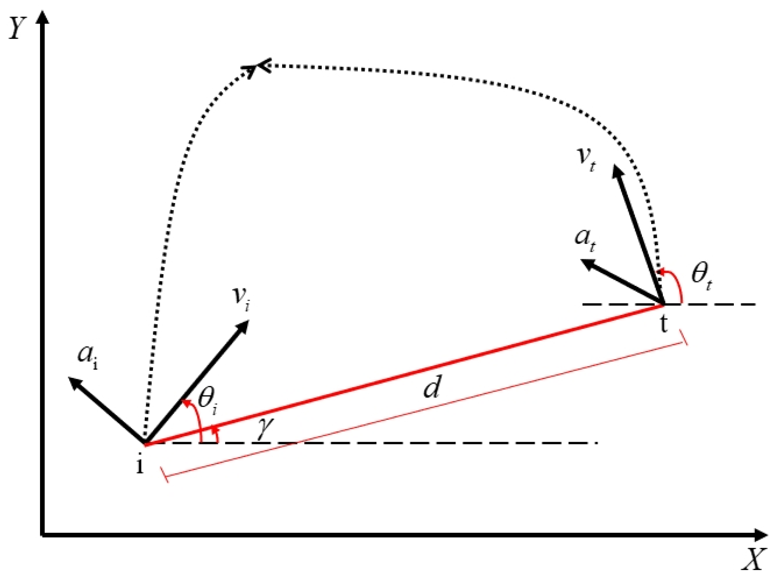
In order to simplify the derivation, both the interceptor and the target are considered as mass points. Both gravity and the aerodynamics model for them are ignored. Specifically, the interceptor and the target are denoted by the symbols of ‘i’ and ‘t’, respectively, and a schematic diagram is provided in Figure 1. To describe the relative motion dynamics, the relative states consist of the LOSA $\gamma \in \mathbb{R}$, the LOSAR $\varpi \in \mathbb{R}$, the relative distance $d\in \mathbb{R}$, and the relative velocity $v_{i-t}\in \mathbb{R}$. ${\theta }_i\in \mathbb{R}$ is the interceptor’s flight-path angles (FPA). ${\theta }_t\in \mathbb{R}$ is the target’s FPA. The velocities of the interceptor and the target are represented by $v_i$ and $v_t$, respectively. Both $v_i$ and $v_t$ are assumed to be constants. All of these are normal components contained in the horizontal plane and can be measured by the seeker of the interceptor.

Figure 1. Relative motion between the interceptor and the target in a two-dimensional system.

In a horizontal plane without air and gravity, the relative kinematical equations for the interceptor–target are given as [33]

$$\left\{\begin{array}{cc}\hfill v_{i-t}& =\dot{d}=v_{t}cos({\theta }_t-\gamma )-v_{i}cos({\theta }_i-\gamma )\hfill \\ \hfill \varpi & =\dot{\gamma }=\frac{1}{d}(v_{t}sin({\theta }_t-\gamma )-v_{i}sin({\theta }_i-\gamma ))\hfill \end{array}\right.$$

(1)

The kinematical equations for the interceptor are given as [33]

$$\left\{\begin{array}{cc}\hfill {\dot{\theta }}_i& =\frac{a_i}{v_i}\hfill \\ \hfill {\dot{x}}_i& =v_{xi}=v_{i}cos{\theta }_i\hfill \\ \hfill {\dot{y}}_i& =v_{yi}=v_{i}sin{\theta }_i\hfill \end{array}\right.$$

(2)

where $x_i\in \mathbb{R}$ and $y_i\in \mathbb{R}$ denote the x-coordinate and y-coordinate of the interceptor, respectively. The velocities along $x_i$ and $y_i$ are $v_{xi}\in \mathbb{R}$ and $v_{yi}\in \mathbb{R}$, respectively. The variable $a_i\in \mathbb{R}$ denotes the interceptor’s acceleration normal to its velocity. All of these are normal components contained in the horizontal plane.

In the same way, the kinematical equations of the target are given as [33]

$$\left\{\begin{array}{cc}\hfill {\dot{\theta }}_t& =\frac{a_t}{v_t}\hfill \\ \hfill {\dot{x}}_t& =v_{xt}=v_{t}cos{\theta }_t\hfill \\ \hfill {\dot{y}}_t& =v_{yt}=v_{t}sin{\theta }_t\hfill \end{array}\right.$$

(3)

where $x_t\in \mathbb{R}$ and $y_t\in \mathbb{R}$ denote the x-coordinate and y-coordinate of the target, respectively. The velocities along $x_t$ and $y_t$ are $v_{xt}\in \mathbb{R}$ and $v_{yt}\in \mathbb{R}$, respectively. $a_t\in \mathbb{R}$ represents the target’s normal acceleration. It is important to point out that all the states mentioned above, except the target’s acceleration $a_t$, can be measured by the seeker of the interceptor. All of them are normal components contained in the horizontal plane.

Considering (1), (2), and (3), the derivative of $\varpi$ is given as [34]

$$\dot{\varpi }=\frac{-2v_{i-t}}{d}\varpi -\frac{a_{i}cos({\theta }_i-\gamma )}{d}+\frac{a_{t}cos({\theta }_t-\gamma )}{d}$$

(4)

Thus, the relative kinematic equations are rewritten as [34]

$$\left\{\begin{array}{cc}\hfill \dot{\gamma }& =\varpi \hfill \\ \hfill \dot{\varpi }& =\frac{-2v_{i-t}}{d}\varpi -\frac{a_{i}cos({\theta }_i-\gamma )}{d}+\frac{\Omega }{d}\hfill \end{array}\right.$$

(5)

where $\Omega =a_{t}cos({\theta }_t-\gamma )$ is the target’s acceleration normal to the LOSAR. Because $a_t$ is unmeasurable, $\Omega$ is treated as a disturbance of the system.

The objective of this paper was to design the interceptor’s acceleration $a_i$ as a control input that can guarantee $\varpi$ remains in a sufficiently small neighborhood to zero. In other words, $\gamma$ rapidly converges to a neighborhood of a suitable constant under the conditions of the LOSA constraint and simultaneously satisfies the performance indexes of the state and control input. Then, if the relative velocity is negative and the LOSAR is stabilized, the interceptor will finally intercept the target [35]. Thus, to realize the PAG, we define the tracking error as $e_{\gamma }=\gamma -{\gamma }_c$ where ${\gamma }_c$ is the constant tracking command of $\gamma$.

The derivative of the tracking error $e_{\gamma }$ with respect to time is given as

$${\dot{e}}_{\gamma }=\varpi$$

(6)

because of the derivative of the tracking command, ${\dot{\gamma }}_c$ is zero for achieving PAG.

In order to carry out follow-up work and take into account the real situation, we made the following assumptions:

Assumption 1.

The target’s normal acceleration $a_t$ is continuous, bounded, and differentiable. And $a_t$ satisfies $\left|\frac{d^i{a}_t}{d{t}^i}\right|\le \alpha ,i=0,1,...$, where $\alpha >0$ is a constant;

Assumption 2

([8]). For the system (5), the LOSAR is controllable when $\left|{\theta }_i-\gamma \right|\ne \frac{\pi }{2}$. Thus, in the guidance process, the LOSA γ and the FGA ${\theta }_i$ of the interceptor remain in the domain Π defined by

$$\mathsf{\Pi }=\left\{\gamma ,{\theta }_i,\in \mathbb{R}:\left|{\theta }_i-\gamma \right|\ne \frac{\pi }{2}\right\}$$

(7)

Remark 1

([8]). The guidance system (5) is unavailable when the relative distance $d\to 0$. In the TGP, considering the limitations of physical factors such as the interceptor seeker and the receiver overload, there is a minimum distance $d_m$; when $d<d_m$, the guidance can be considered to end, then the interceptor and the target rely on their own inertia to complete the final guidance task.

Remark 2.

Considering the field of view of the interceptor’s seeker and the performance of the interception, the LOSA is required to be always in the feasible region $\Xi =\left\{\gamma \in \mathbb{R}:{\gamma }_l\le \gamma \le {\gamma }_u\right\}$, where ${\gamma }_l$ and ${\gamma }_u$ are the lower and upper bounds of the region. In this feasible domain, the seeker can measure the system state information at all times. If the LOSA is not in this region, this could cause the escape of the target and thus cause the failure of the interception mission.

3. Finite-Time Prescribed Performance and DSDO-Based Guidance

In this section, PAG is realized using a DSDO and FPPC. The unmeasured target maneuver is estimated by the DSDO and the estimation is fed forward into the system. To improve the interception accuracy, an DSDO is designed whose estimation accuracy is independent of the relative distance. A PAG law is proposed using the FPPC, so that the LOSAR converges to the neighborhood of zero in a specified finite time. The rapid performance and transient performance of the guidance system are ensured.

3.1. Finite-Time Prescribed Performance

The faster the LOSAR converges, the better the speed of the guidance system. Therefore, FPPC is a suitable method for designing a PAG law. In view of the disadvantage of a large overshoot affecting the performance, a finite-time performance function (FTPF) is employed. Considering the seeker’s measurement area and the quality of the PAG, the LOSA error $e_{\gamma }$ converges to a bounded region, constrained as follows:

$${\omega }_l\left(t\right)<e_{\gamma }<{\omega }_u\left(t\right)$$

(8)

where ${\omega }_l\in \mathbb{R}$ and ${\omega }_u\in \mathbb{R}$ are the FTPFs. Due to the advantages of PPC, the tracking error can be limited to the preset upper and lower bounds. During the whole guidance process, the LOSA error $e_{\gamma }$ is limited to the FTPFs ${\omega }_l$ and ${\omega }_u$; that is, ${\omega }_l<\gamma -{\gamma }_c<{\omega }_u$. Thus, the LOSA is restricted between ${\omega }_l+{\gamma }_c$ and ${\omega }_u+{\gamma }_c$. The LOSA is required to be within the region $\Xi$ to achieve a good performance for the guidance system, so the choice of FTPFs should satisfy the inequality, which is given as

$${\gamma }_l<{\omega }_l+{\gamma }_c<{\omega }_u+{\gamma }_c<{\gamma }_u$$

(9)

Due to the advantages of PPC, the LOSA is maintained in the region $\Xi$ during the guidance process. The escape of the target is avoided.

The FTPFs ${\omega }_l$ and ${\omega }_u$ are chosen as [32]

$$\begin{array}{cc}\hfill {\omega }_l=& \left\{\begin{array}{c}{\gamma }_0\left[\mathrm{sign}\left(e_{\gamma }\left(0\right)\right)-{\rho }_l\right]exp\left(\frac{-\tau t}{T_F-t}\right)-{\rho }_l{\gamma }_{l,F},t\in \left[0,T_F\right)\hfill \\ -{\rho }_l{\gamma }_{l,F},t\in \left[T_F,\infty \right)\hfill \end{array}\right.\hfill \\ \hfill {\omega }_u=& \left\{\begin{array}{c}{\gamma }_0\left[\mathrm{sign}\left(e_{\gamma }\left(0\right)\right)-{\rho }_u\right]exp\left(\frac{-\tau t}{T_F-t}\right)-{\rho }_u{\gamma }_{u,F},t\in \left[0,T_F\right)\hfill \\ -{\rho }_u{\gamma }_{u,F},t\in \left[T_F,\infty \right)\hfill \end{array}\right.\hfill \end{array}$$

(10)

where ${\rho }_l\in \left(0,1\right)$, ${\rho }_u\in \left(0,1\right)$, ${\gamma }_0>0$, ${\gamma }_{l,F}>0$, ${\gamma }_{u,F}>0$, $\tau >0$ and $T_F>0$ are the constants to be determined, and $e_{\gamma }\left(0\right)$ is the initial value of the LOSA error. ${\gamma }_{l,F}<{\gamma }_0$ and ${\gamma }_{u,F}<{\gamma }_0$. Correct choice of the above parameters is required to ensure that the inequality (8) is valid.

Remark 3.

The parameter τ determines the convergence speed of the FTPFs. The specified finite time $T_F$ determines the convergence time of the LOSAR. In this way, the speed of the guidance system is ensured.

Because of the requirement to ensure that the LOSA error can converge before the end of the guidance, attention should be paid to the selection of $T_F$. The time-to-go of the PAG is given as

$$\begin{array}{c}\hfill t_{ttg}=\frac{d_m-d\left(t\right)}{v_{m-t}}\end{array}$$

(11)

where $d_m$ is the minimum distance.

To make the LOSA error converge to a suitable time, the value of $T_F$ is approximately chosen as

$$\begin{array}{c}\hfill T_F=f_r{t}_{ttg0}\end{array}$$

(12)

where $t_{ttg0}$ is the initial value of the time-to-go and $f_r\in (0,1)$ is a suitable constant.

Remark 4.

Since the signs of the FTPFs are related to the initial LOSA error, the sign of the LOSA error $e_{\gamma }$ remains unchanged in the process of realizing the PAG. This will not only give the system a smaller overshoot but also facilitates the seeker in measuring information during the interception process. This improvement in the measurement quality plays a pivotal role in the improvement in the interception accuracy.

To proceed further, the derivatives of ${\omega }_l$ and ${\omega }_u$ with respect to time are given as

$$\begin{array}{cc}\hfill {\dot{\omega }}_l=& \left\{\begin{array}{c}\frac{-{\gamma }_0\tau T_F}{{\left(T_F-t\right)}^2}\left[\mathrm{sign}\left(e_{\gamma }\left(0\right)\right)-{\rho }_l\right]exp\left(\tau \frac{-t}{T_F-t}\right),t\in \left[0,T_F\right)\hfill \\ 0,t\in \left[T_F,\infty \right)\hfill \end{array}\right.\hfill \\ \hfill {\dot{\omega }}_u=& \left\{\begin{array}{c}\frac{-{\gamma }_0\tau T_F}{{\left(T_F-t\right)}^2}\left[\mathrm{sign}\left(e_{\gamma }\left(0\right)\right)-{\rho }_u\right]exp\left(\tau \frac{-t}{T_F-t}\right),t\in \left[0,T_F\right)\hfill \\ 0,t\in \left[T_F,\infty \right)\hfill \end{array}\right.\hfill \end{array}$$

(13)

The second-order derivatives of FTPFs are given as

$$\begin{array}{cc}\hfill {\ddot{\omega }}_l=& \left\{\begin{array}{c}\frac{{\gamma }_0\left({\tau }^2{T}_F^2-2\tau T_F\left(T_F-t\right)\right)}{{\left(T_F-t\right)}^4}\left(\mathrm{sign}\left(e_{\gamma }\left(0\right)\right)-{\rho }_l\right)exp\left(\tau \frac{-t}{T_F-t}\right),t\in \left[0,T_F\right)\hfill \\ 0,t\in \left[T_F,\infty \right)\hfill \end{array}\right.\hfill \\ \hfill {\ddot{\omega }}_u=& \left\{\begin{array}{c}\frac{{\gamma }_0\left({\tau }^2{T}_F^2-2\tau T_F\left(T_F-t\right)\right)}{{\left(T_F-t\right)}^4}\left(\mathrm{sign}\left(e_{\gamma }\left(0\right)\right)-{\rho }_u\right)exp\left(\tau \frac{-t}{T_F-t}\right),t\in \left[0,T_F\right)\hfill \\ 0,t\in \left[T_F,\infty \right)\hfill \end{array}\right.\hfill \end{array}$$

(14)

Based on the design flow of the prescribed performance, we convert $e_{\gamma }$ into the unconstrained error $\upsilon$, which is expressed as [32]

$$\upsilon =ln\left(\frac{e_{\gamma }-{\omega }_l}{{\omega }_u-e_{\gamma }}\right)$$

(15)

where $\upsilon$ satisfies $\underset{e_{\gamma }\to {\omega }_l}{lim}\upsilon =-\infty$, $\underset{e_{\gamma }\to {\omega }_u}{lim}\upsilon =\infty$. Considering that the $\mathsf{\Theta }\left(e_{\gamma }\right)=ln\left(\frac{e_{\gamma }-{\omega }_l}{{\omega }_u-e_{\gamma }}\right)$ is a monotonically increasing function of the LOSA error, any LOSA error $e_{\gamma }\in ({\omega }_l\left(t\right),{\omega }_u\left(t\right))$ uniquely corresponds to an unconstrained error $\upsilon \in (-\infty ,\infty )$. The task of controlling the constrained error can be transformed into the task of controlling unconstrained error. In this regard, controlling an unconstrained error greatly reduces the difficulty of control. There is no need to worry about interception failure due to an excessive absolute value of LOSA.

The derivative of $\upsilon$ respect to time is given as

$$\begin{array}{cc}\hfill \dot{\upsilon }& =\eta \left({\dot{e}}_{\gamma }+\frac{\left({\dot{\omega }}_l-{\dot{\omega }}_u\right)e_{\gamma }+{\dot{\omega }}_u{\omega }_l-{\omega }_u{\dot{\omega }}_l}{{\omega }_u-{\omega }_l}\right)\hfill \\ \hfill & =\eta \left(\varpi +\frac{\left({\dot{\omega }}_l-{\dot{\omega }}_u\right)e_{\gamma }+{\dot{\omega }}_u{\omega }_l-{\omega }_u{\dot{\omega }}_l}{{\omega }_u-{\omega }_l}\right)\hfill \end{array}$$

(16)

with $\eta =\frac{{\omega }_u-{\omega }_l}{\left(e_{\gamma }-{\omega }_l\right)\left({\omega }_u-e_{\gamma }\right)}$.

Now, the objective to converge the constrained $\varpi$ to the neighborhood of zero is transformed into stabilizing the unconstrained error $\upsilon$.

3.2. Distance Scalar Disturbance Observer

Generally speaking, the unknown target maneuver is usually treated as the compound disturbance $\varrho =\frac{\Omega }{d}$. However, when the interceptor nears the target, due to the extremely small relative distance, the derivative of the compound disturbance $\varrho$ will approach infinity. Obviously, the estimation accuracy is seriously affected. Therefore, we project the target acceleration into the LOS coordinate frame and estimate the target’s acceleration normal to the LOSAR $\Omega$ by designing an DSDO. The estimation accuracy is better, regardless of the relative distance.

The DSDO is designed as

$$\begin{array}{c}\hfill \left\{\begin{array}{cc}\hfill \widehat{\Omega }& =\widehat{z}+n\varpi d\hfill \\ \hfill \dot{\widehat{z}}& =n(\varpi v_{i-t}+a_{i}cos({\theta }_i-\gamma )-\widehat{\Omega })\hfill \end{array}\right.\end{array}$$

(17)

where $n>0$ is a constant, z is an intermediate variable, and $z=\Omega -n\varpi d$.

The derivative of z is given as

$$\dot{z}=\dot{\Omega }-n\varpi \dot{d}-nd\dot{\varpi }$$

(18)

Substituting (5) into (18) yields

$$\dot{z}=\dot{\Omega }+n\left(\varpi v_{i-t}+a_{i}cos\left({\theta }_i-\gamma \right)-\Omega \right)$$

(19)

The derivative of the disturbance $\Omega$ is given as

$$\dot{\Omega }={\dot{a}}_{t}cos\left({\theta }_t-\gamma \right)-a_{t}sin\left({\theta }_t-\gamma \right)\left({\dot{\theta }}_t-\dot{\gamma }\right)$$

(20)

and then, substituting (1) and (3) into (20) yields

$$\begin{array}{cc}\hfill \dot{\Omega }=& -\frac{sin\left({\theta }_t-\gamma \right)}{v_t}{a}_t^2+\frac{v_t{sin}^2({\theta }_t-\gamma )}{d}{a}_t\hfill \\ \hfill & -\frac{v_{i}sin({\theta }_i-\gamma )sin\left({\theta }_t-\gamma \right)}{d}{a}_t+{\dot{a}}_{t}cos\left({\theta }_t-\gamma \right)\hfill \end{array}$$

(21)

Recalling that both $v_m$ and $v_t$ are constant and $\left|\frac{d^i{a}_t}{d{t}^i}\right|\le \alpha ,i=0,1,...$, it is obtained that

$$\begin{array}{cc}\hfill \left|\dot{\Omega }\right|& \le \frac{a_t^2}{v_t}+\frac{v_t}{d}\alpha +\frac{v_i}{d}\alpha +\alpha \hfill \\ \hfill & \le \frac{a_t^2}{v_t}+\frac{v_t+v_i+d}{d}\alpha \hfill \\ \hfill & \le \frac{{\alpha }^2}{v_t}+\frac{v_t+v_i}{d_m}\alpha +\alpha \hfill \end{array}$$

(22)

Since the right side of the inequality sign consists of constant terms, the derivative of the disturbance $\dot{\Omega }$ is bounded.

Considering the stability of the DSDO, the error of estimation is defined as

$$\begin{array}{c}\hfill \tilde{\Omega }=\Omega -\widehat{\Omega }\end{array}$$

(23)

The derivative of $\tilde{\Omega }$ is developed as

$$\begin{array}{cc}\hfill \dot{\tilde{\Omega }}& =\dot{\Omega }+n\left(\varpi v_{i-t}+a_{i}cos\left({\theta }_i-\gamma \right)-\Omega \right)-n\left(\varpi v_{i-t}+a_{i}cos\left({\theta }_i-\gamma \right)-\widehat{\Omega }\right)\hfill \\ \hfill & =\dot{\Omega }-n\left(\Omega -\widehat{\Omega }\right)\hfill \\ \hfill & =\dot{\Omega }-n\tilde{\Omega }\hfill \end{array}$$

(24)

where $\dot{\Omega }$ is bounded and $n>0$. Thus, the estimation error will converge to a bounded region, and the designed DSDO can track the unknown disturbance.

Remark 5.

This paper provides a design idea for target maneuver estimation that is not limited to a two-dimensional coordinate system. When considering the interception problem of a maneuvering target in a three-dimensional coordinate system, the target acceleration can still be projected onto two components perpendicular to the line-of-sight (LOS) under the LOS frame. In this way, the decoupling of the disturbance and relative distance is realized, and the decline in the estimation accuracy is avoided when the interceptor is near the target.

3.3. Parallel Approaching Guidance Design

As above, the LOSA error $e_{\gamma }$ is converted to an unconstrained $\upsilon$ using an error transformation function, and the projected target acceleration is estimated by the DSDO using the system states. In order to achieve PAG, we use the system states and the estimation $\widehat{\Omega }$ to design a PAG law that can stabilize $\upsilon$ and then input the PAG law into the interception system. The structure of the interception system of this paper is shown in the Figure 2. Considering the principle of the PAG making the LOSAR remain zero, the PAG law is obtained using the method of backstepping. To proceed further, we define $z_1=\upsilon$, $z_2=\varpi -{\sigma }_c$, where ${\sigma }_c$ is a virtual law to be designed. To stabilize the transformed error, just like in the common stability analysis process, we define $V_1=\frac{1}{2}{z}_1^2$, and its derivative is given as

$$\begin{array}{cc}\hfill {\dot{V}}_1& =z_1\eta \left(\varpi +\frac{\left({\dot{\omega }}_l-{\dot{\omega }}_u\right)e_{\gamma }+{\dot{\omega }}_u{\omega }_l-{\omega }_u{\dot{\omega }}_l}{{\omega }_u-{\omega }_l}\right)\hfill \\ \hfill & =z_1\eta \left(z_2+{\sigma }_c+\frac{\left({\dot{\omega }}_l-{\dot{\omega }}_u\right)e_{\gamma }+{\dot{\omega }}_u{\omega }_l-{\omega }_u{\dot{\omega }}_l}{{\omega }_u-{\omega }_l}\right)\hfill \end{array}$$

(25)

Figure 2. FPPC-based PAG system structure diagram.

We design the stabilizing function ${\sigma }_c$ as

$$\begin{array}{c}\hfill {\sigma }_c=-\frac{k_1{z}_1}{\eta }-\frac{\left({\dot{\omega }}_l-{\dot{\omega }}_u\right)e_{\gamma }+{\dot{\omega }}_u{\omega }_l-{\omega }_u{\dot{\omega }}_l}{{\omega }_u-{\omega }_l}\end{array}$$

(26)

where $k_1>0$ is a constant. In fact, ${\sigma }_c$ can be understood as the desired LOSAR, which can stabilize $\upsilon$.

Inserting (26) into (25) yields

$${\dot{V}}_1=-k_1{z}_1^2+\eta z_1{z}_2$$

(27)

We define the stability function as

$$V_2=V_1+\frac{1}{2}{z}_2^2$$

(28)

To proceed further, the derivative of $V_2$ is given as

$$\begin{array}{cc}\hfill {\dot{V}}_2& =-k_1{z}_1^2+\eta z_1{z}_2+z_2\left(\dot{\varpi }-{\dot{\sigma }}_c\right)\hfill \\ \hfill & =-k_1{z}_1^2+\eta z_1{z}_2+z_2\left(-\frac{2v_{i-t}}{d}\varpi +\frac{1}{d}\Omega -{\dot{\sigma }}_c\right.\left.-\frac{cos\left({\theta }_i-\gamma \right)}{d}{a}_i\right)\hfill \end{array}$$

(29)

The derivative of the variable ${\sigma }_c$ is given as

$$\begin{array}{cc}\hfill {\dot{\sigma }}_c& =\frac{k_1\dot{\upsilon }\eta -\upsilon \dot{\eta }}{{\eta }^2}-\frac{\left({\ddot{\omega }}_l-{\ddot{\omega }}_u\right)e_{\gamma }+\left({\omega }_l-{\omega }_u\right)\varpi +{\ddot{\omega }}_u{\omega }_l-{\omega }_u{\ddot{\omega }}_l}{\left({\omega }_u-{\omega }_l\right)}\hfill \\ \hfill & -\frac{\left({\dot{\omega }}_l-{\dot{\omega }}_u\right)\left[\left({\dot{\omega }}_l-{\dot{\omega }}_u\right)e_{\gamma }+{\dot{\omega }}_u{\omega }_l-{\omega }_u{\dot{\omega }}_l\right]}{{\left({\omega }_u-{\omega }_l\right)}^2}\hfill \end{array}$$

(30)

where $\dot{\eta }=\frac{{\dot{\omega }}_l-{\dot{\omega }}_u}{\left(e_{\gamma }-{\omega }_l\right)\left({\omega }_u-e_{\gamma }\right)}-\frac{\left(\varpi -{\dot{\omega }}_l\right)\left({\dot{\omega }}_u-\varpi \right)\left({\omega }_u-{\omega }_l\right)}{{\left(e_{\gamma }-{\omega }_l\right)}^2{\left({\omega }_u-e_{\gamma }\right)}^2}$.

To stabilize the transformed error and the LOSAR, we design the PAG law as

$$\begin{array}{cc}\hfill a_i& =\frac{d}{cos\left({\theta }_i-\gamma \right)}\left(-\frac{2v_{i-t}}{d}\varpi -{\dot{\sigma }}_c+k_2{z}_2+\eta z_1\right.\left.+\frac{1}{d}\widehat{\Omega }+\frac{{\lambda }_1{z}_2}{2d^2}\right)\hfill \end{array}$$

(31)

where $\frac{{\lambda }_1{z}_2}{2d^2}$ is the stability term, which will be mentioned below, and ${\lambda }_1>0$ is a regulation factor.

In this way, the LOSAR is stabilized within the given time $T_F$ and remains in a small enough neighborhood of zero until the end of guidance. The implementation mechanism of the PAG is shown in Figure 3.

Figure 3. The implementation of PAG using FPPC.

4. Stability Analysis

According to the principle of PAG, if the LOSA error and the estimation error can guarantee UUB, the feasibility of the guidance law can be verified. In this section, the stabilities of the LOSA error and the estimation error are analyzed. This analysis leads to a theorem, as follows:

Theorem 1.

For the system (5), in the presence of the DSDO (17) and the PAG law (30) based on the FPPC, the signal $z_1$, $z_2$ and the estimation error $\tilde{\Omega }$ are UUB and the PAG is realized when the constants $k_1$, $k_2$, and n satisfy the conditions

$$\left\{\begin{array}{cc}\hfill k_1& >0\hfill \\ \hfill k_2& >0\hfill \\ \hfill n& >\frac{1}{2{\lambda }_1}+\frac{{\lambda }_2}{2}\hfill \end{array}\right.$$

(32)

where ${\lambda }_2>0$ is a regulation factor.

Proof of Theorem 1.

Considering the estimation error of the DSDO, we define the stability function of the guidance system (5) as

$$V=V_2+\frac{1}{2}{\tilde{\Omega }}^2$$

(33)

To discuss the role of the PAG law in stabilizing the signals $z_1$ and $z_2$, we substitute (31) into (29), and the derivative of $V_2$ is rewritten as

$$\begin{array}{c}\hfill {\dot{V}}_2=-k_1{z}_1^2-k_2{z}_2^2+\frac{z_2}{d}\left(\Omega -\widehat{\Omega }\right)-\frac{{\lambda }_1{z}_2^2}{2d^2}\end{array}$$

(34)

Using Young’s inequality, one has

$$\begin{array}{cc}\hfill {\dot{V}}_2& \le -k_1{z}_1^2-k_2{z}_2^2+\frac{{\lambda }_1{z}_2^2}{2d^2}+\frac{1}{2{\lambda }_1}{\tilde{\Omega }}^2-\frac{{\lambda }_1{z}_2^2}{2d^2}\hfill \\ \hfill & \le -k_1{z}_1^2-k_2{z}_2^2+\frac{1}{2{\lambda }_1}{\tilde{\Omega }}^2\hfill \end{array}$$

(35)

As long as we can prove the boundedness of $\tilde{\Omega }$, we can guarantee that $z_1$ and $z_2$ will be stabilized. Taking the derivative of (33) and substituting (24) into it, we can obtain

$$\begin{array}{cc}\hfill \dot{V}& \le -k_1{z}_1^2-k_2{z}_2^2+\frac{1}{2{\lambda }_1}{\tilde{\Omega }}^2+\tilde{\Omega }\dot{\tilde{\Omega }}\hfill \\ \hfill & \le -k_1{z}_1^2-k_2{z}_2^2+\frac{1}{2{\lambda }_1}{\tilde{\Omega }}^2+\tilde{\Omega }\left(\dot{\Omega }-n\tilde{\Omega }\right)\hfill \\ \hfill & \le -k_1{z}_1^2-k_2{z}_2^2-\left(n-\frac{1}{2{\lambda }_1}\right){\tilde{\Omega }}^2+\tilde{\Omega }\dot{\Omega }\hfill \end{array}$$

(36)

Using Young’s inequality, the inequality (36) becomes

$$\begin{array}{cc}\hfill \dot{V}& \le -k_1{z}_1^2-k_2{z}_2^2-\left(n-\frac{1}{2{\lambda }_1}\right){\tilde{\Omega }}^2+\frac{{\lambda }_2}{2}{\tilde{\Omega }}^2+\frac{1}{2{\lambda }_2}{\dot{\Omega }}^2\hfill \\ \hfill & \le -k_1{z}_1^2-k_2{z}_2^2-\left(n-\frac{1}{2{\lambda }_1}-\frac{{\lambda }_2}{2}\right){\tilde{\Omega }}^2+\frac{1}{2{\lambda }_2}{\dot{\Omega }}^2\hfill \\ \hfill & \le -k_1{z}_1^2-k_2{z}_2^2-\left(n-\frac{1}{2{\lambda }_1}-\frac{{\lambda }_2}{2}\right){\tilde{\Omega }}^2+\frac{1}{2{\lambda }_2}{\left|\dot{\Omega }\right|}^2\hfill \end{array}$$

(37)

where ${\lambda }_2$ is a positive regulation factor.

Taking into account the above proof of the boundedness of $\dot{\Omega }$, we substitute the proof result (22) into (37). The derivative of the stability function V is rewritten as

$$\begin{array}{cc}\hfill \dot{V}& \le -k_1{z}_1^2-k_2{z}_2^2-\left(n-\frac{1}{2{\lambda }_1}-\frac{{\lambda }_2}{2}\right){\tilde{\Omega }}^2+\frac{1}{2{\lambda }_2}{\left(\frac{{\alpha }^2}{v_t}+\frac{v_t+v_i}{d_m}\alpha +\alpha \right)}^2\hfill \\ \hfill & \le -\kappa V+C\hfill \end{array}$$

(38)

where $\kappa$ and C are given as

$$\begin{array}{c}\hfill \begin{array}{c}\kappa :=min\left(\begin{array}{c}{\lambda }_{min}\left(k_1\right)\\ {\lambda }_{min}\left(k_2\right)\\ {\lambda }_{min}\left(n-\frac{1}{2{\lambda }_1}-\frac{{\lambda }_2}{2}\right)\end{array}\right)\hfill \\ C:=\frac{1}{2{\lambda }_2}{\left(\frac{{\alpha }^2}{v_t}+\frac{v_t+v_i}{d_m}\alpha +\alpha \right)}^2\hfill \end{array}\end{array}$$

(39)

If $k_1$, $k_2$, and n satisfy the condition (32), according to (38) one has

$$\begin{array}{c}\hfill 0\le V\le \left[V\left(0\right)-\frac{C}{\kappa }\right]e^{-\kappa t}+\frac{C}{\kappa }\end{array}$$

(40)

where $V\left(0\right)=\frac{1}{2}{z}_1^2\left(0\right)+\frac{1}{2}{z}_2^2\left(0\right)+\frac{1}{2}{\tilde{\Omega }}^2\left(0\right)$.

From the definition of the Lyapunov function V, we have [35]

$$\begin{array}{c}\hfill \begin{array}{cc}\hfill \left|z_1\right|& \le \sqrt{2\left[V\left(0\right)-\frac{C}{\kappa }\right]e^{-\kappa t}+\frac{2C}{\kappa }}\hfill \\ \hfill \left|z_2\right|& \le \sqrt{2\left[V\left(0\right)-\frac{C}{\kappa }\right]e^{-\kappa t}+\frac{2C}{\kappa }}\hfill \\ \hfill \left|\tilde{\Omega }\right|& \le \sqrt{2\left[V\left(0\right)-\frac{C}{\kappa }\right]e^{-\kappa t}+\frac{2C}{\kappa }}\hfill \end{array}\end{array}$$

(41)

From (41), we can conclude that for any $t\ge T$, we have $\left|z_1\right|\le D$, $\left|z_2\right|\le D$, and $\left|\tilde{\Omega }\right|\le D$ where [35]

$$\begin{array}{c}\hfill D=\sqrt{2\left[V\left(0\right)-\frac{C}{\kappa }\right]e^{-\kappa T}+\frac{2C}{\kappa }}\end{array}$$

(42)

Then, we have [35]

$$\begin{array}{c}\hfill T=-\frac{1}{\kappa }ln\left(\frac{D_1^2-\frac{2C}{\kappa }}{2\left[V\left(0\right)-\frac{C}{\kappa }\right]}\right)\end{array}$$

(43)

In addition, from (40) we can determine that

$$\begin{array}{c}\hfill \underset{t\to \infty }{lim}V\le \frac{C}{\kappa }\end{array}$$

(44)

This means the signals $z_1$, $z_2$ and $\tilde{\Omega }$ are UUB [18]. This completes the proof. □

5. Simulation Results

To prove the feasibility of the PAG law, three scenarios were considered in this section. In addition, the guidance performances of the PAG law in the three scenarios were compared with those of PNG. The selections of the initial system states and the controller parameters are given in Table 1 and Table 2. The simulation results for the three Scenarios were as follows:

Table 1. The initial values of the guidance system states.

System States	Initial Value
$(x_{m0},y_{m0})$	$(0,0)$ (m)
$(x_{t0},y_{t0})$	$(3600,3600)$ (m)
$v_m$	530 (m/s)
$v_t$	410 (m/s)
${\theta }_{m0}$	$\frac{65\pi }{180}$ (rad/s)
${\theta }_{t0}$	0 (rad/s)
${\gamma }_c$	$\frac{20\pi }{180}$(rad/s)

Table 2. The values of the controller parameters.

System States	Initial Value
$k_1$	3
$k_2$	10
n	100
${\gamma }_0$	$1.4543$
${\rho }_l$	$0.85$
${\rho }_u$	$0.55$
$T_F$	$9.2$
$\tau$	$1.89$
${\gamma }_{l,F}$	$0.0471$
${\gamma }_{u,F}$	$0.0727$

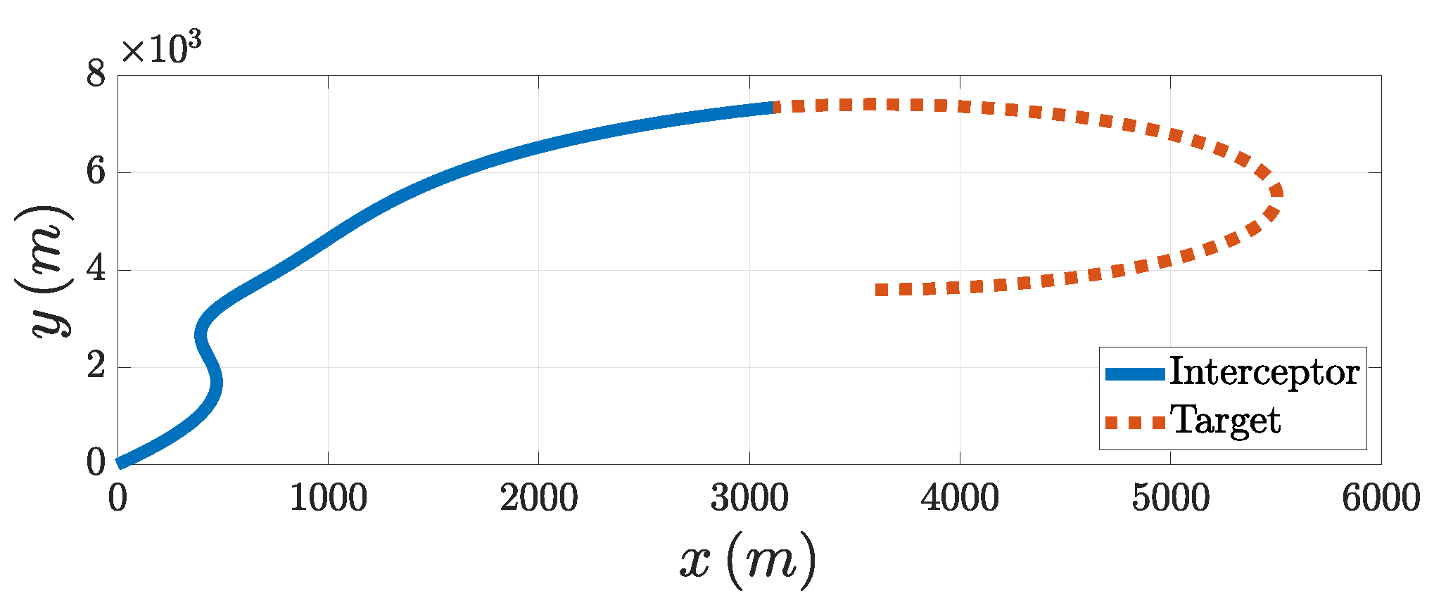
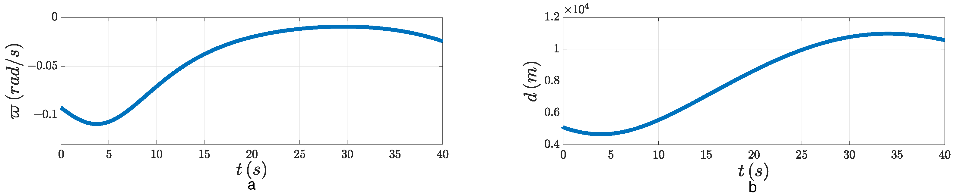
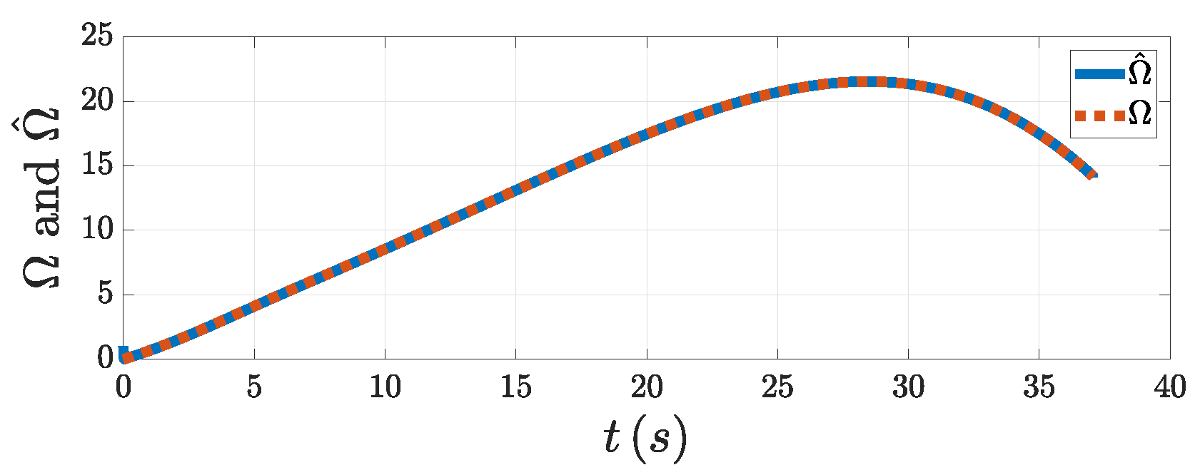
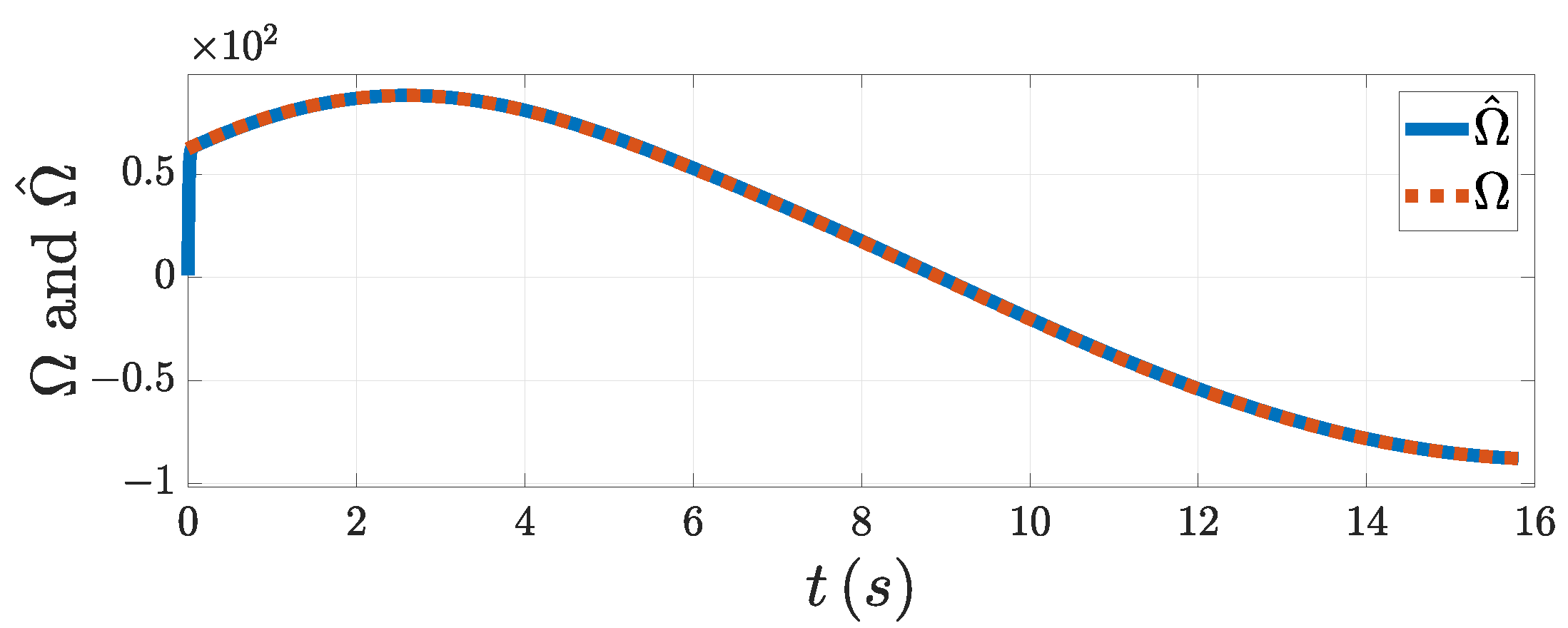
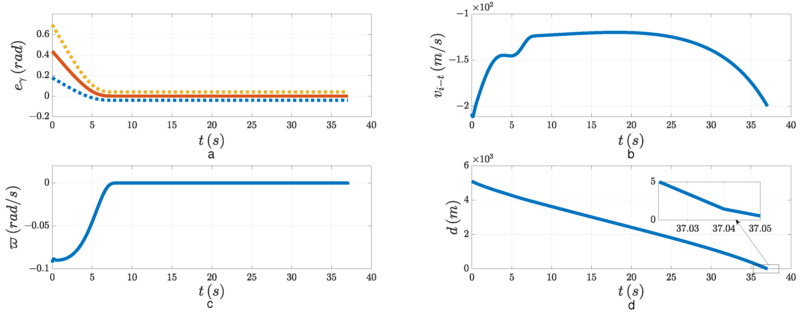
Scenario 1 (Constant Acceleration): The acceleration of the target is given by $a_t=9$ g. Considering the target for a circular maneuver, $a_t=9$ g, when $a_i=0$. It is apparent that the LOSAR was not stabilized, and the minimum distance could not be reached, see Figure 4. That means the interception was unsuccessful when $a_i=0$. Then, we fed the FPPC-based guidance law into the system. From Figure 5, the DSDO could track the target’s maneuver well using the designed PAG law. This means that the influence of the target maneuver on the guidance accuracy could be compensated for well after the estimation of DSDO was input into the system. From Figure 6a,c, both the tracking error and the LOSAR were stabilized with the FPPC in the specified finite time $T_F$. As can be seen in Figure 4a, the overshoot of the tracking error was small. That means that the smooth change in LOSA gave the system a good performance. 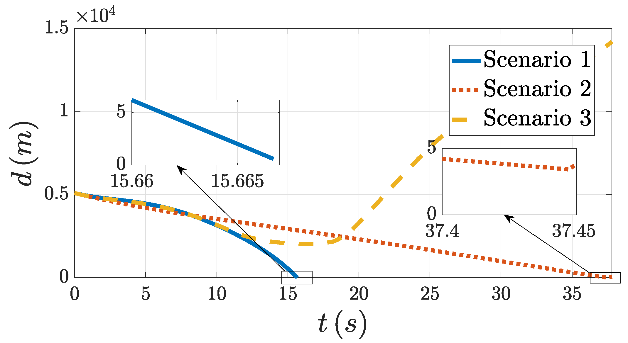If the relative velocity is negative, that is, $v_{i-t}<0$, when the LOSAR remains in a small enough neighborhood of origin, PAG will be realized. From Figure 6b, the relative velocity was negative when the LOSAR was stabilized. In Figure 6d, the relative distance finally converged to the minimum distance. 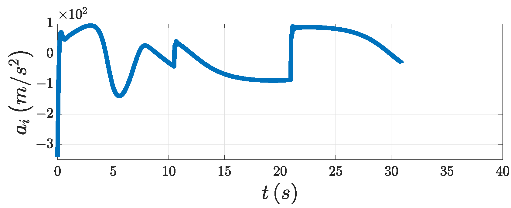The miss distance is shown in Table 3. The PAG law is presented in Figure 7. In addition, in Figure 8, we can see the trajectories of both the interceptor and the target. Therefore, the effectiveness of the PAG law was illustrated when the target performed a circular maneuver.

Figure 4. Signals of the interception system without guidance law in Scenario 1: (a) The LOSAR; (b) The relative distance.

Figure 5. The disturbance and its estimation in Scenario 1.

Figure 6. Closed-loop signals of the interception system in Scenario 1: (a) The LOSA error; (b) The relative velocity; (c) The LOSAR; (d) The relative distance.

Table 3. The guidance accuracies of the different guidance laws in the different scenarios.

Scenarios	Miss Distance of PNG (m)	Miss Distance of PAG (m)
$Scenario1$	$0.6369$	$0.1579$
$Scenario2$	$3.419$	$0.5503$
$Scenario3$	$Miss$	$0.1219$

Figure 7. The interceptor’s acceleration in Scenario 1.

Figure 8. Engagement trajectory in Scenario 1.

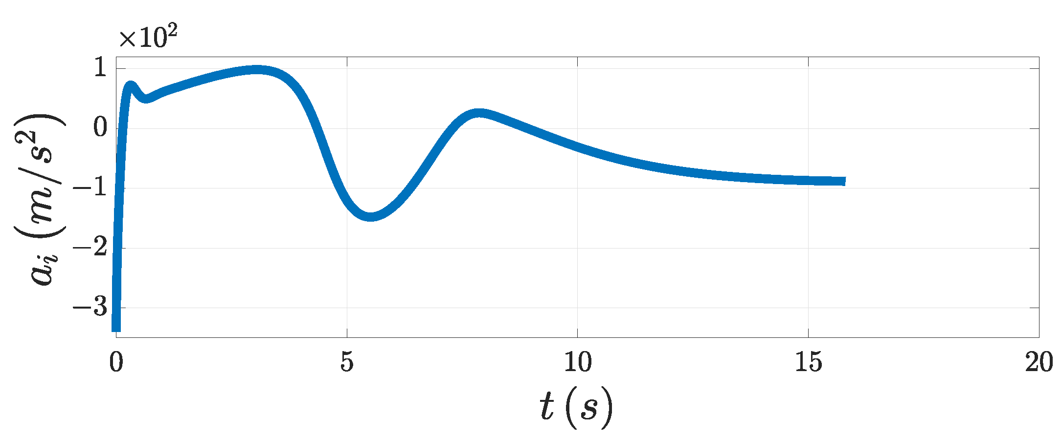
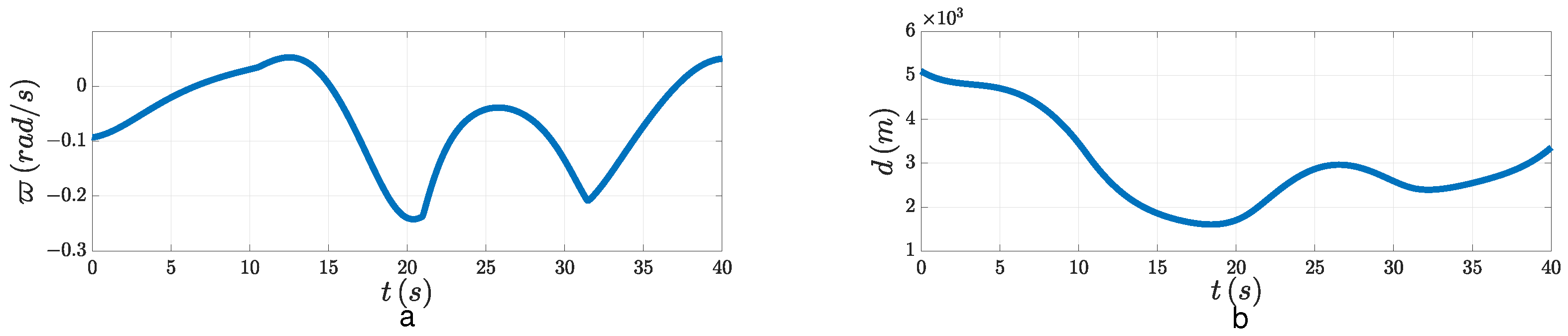
Scenario 2 (Sine Acceleration): The acceleration of the target was set to $a_t=9$ g $sin\left(0.01t\right)$. For the follow-up comparison, we considered a situation where $a_i=0$. It is apparent that the LOSAR was not stabilized and the minimum distance could not be achieved, see Figure 9. That means the interception was unsuccessful when $a_i=0$. From Figure 10, the DSDO could track the target’s maneuver well using the PAG law. That means that the influence of the target maneuver on the guidance accuracy could be well compensated for after the estimation of DSDO was input into the system. From Figure 11a,c, both the tracking error and the LOSAR were stabilized with the FPPC within the specified finite time $T_F$. As can be seen in Figure 11a, the overshoot of the tracking error was small. That means that the smooth change in LOSA gave the system a good performance. From Figure 11b, the relative velocity was negative when the LOSAR remained in the neighborhood of zero. As seen in Figure 11d, the relative distance finally converged to the minimum distance. The PAG law is shown in Figure 12. In addition, from Figure 13 we can see the trajectories of both the interceptor and the target. Therefore, the effectiveness of the PAG law is illustrated.

Figure 9. Signals of the interception system without guidance law in Scenario 2: (a) The LOSAR; (b) The relative distance.

Figure 10. The disturbance and its estimation in Scenario 2.

Figure 11. Closed-loop signals of the interception system in Scenario 2: (a) The LOSA error; (b) The relative velocity; (c) The LOSAR; (d) The relative distance.

Figure 12. The interceptor’s acceleration in Scenario 2.

Figure 13. Engagement trajectory in Scenario 2.

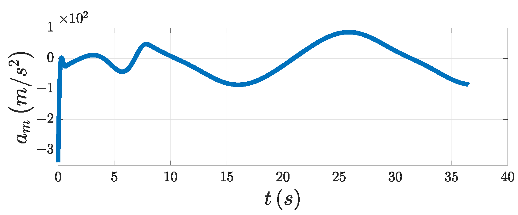
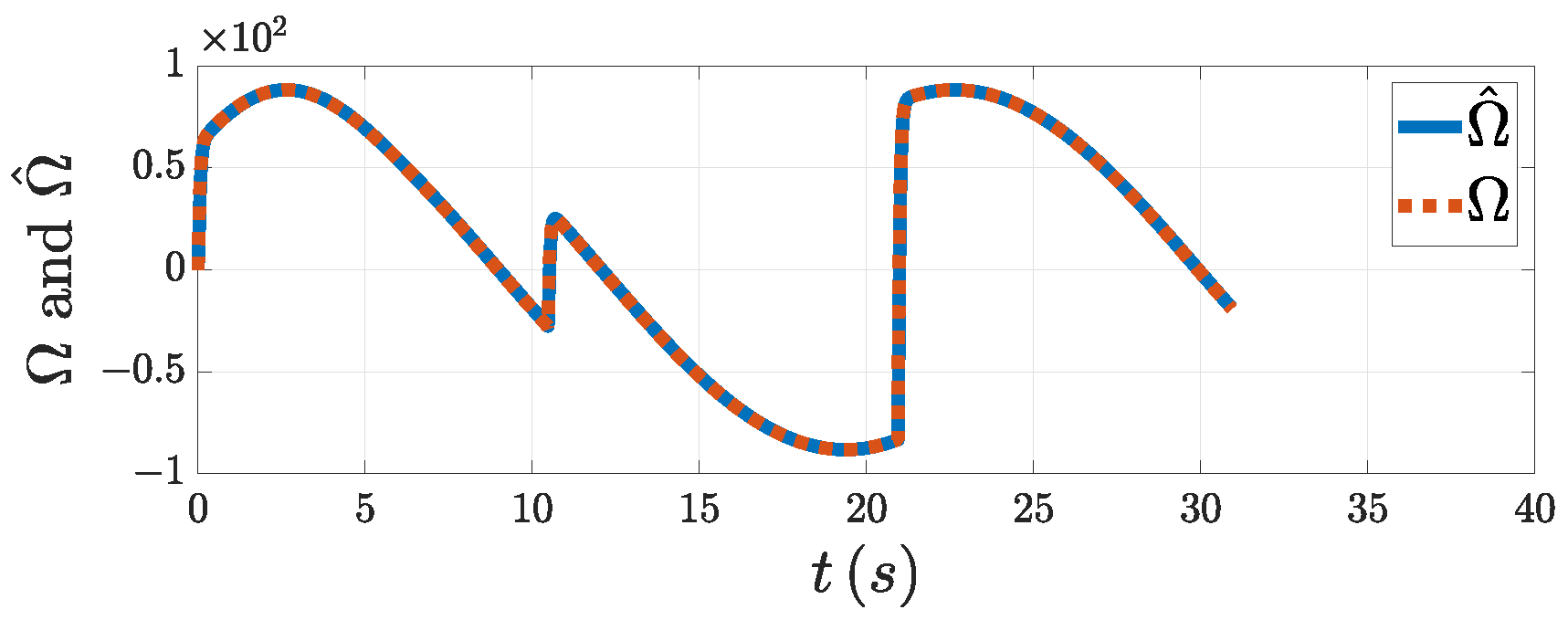
Scenario 3 (Square-Like Acceleration): The acceleration of the target $a_t$ was given by a square-like signal, the amplitude of the signal was 9 g, and the frequency was $0.3$ rad/s. Considering the target for a square-like maneuver when $a_i=0$, the LOSAR and the relative distance were as shown in Figure 14. The interception was unsuccessful when $a_i=0$. As seen in Figure 15, the DSDO could track the target’s maneuver well using the PAG law. That means the influence of the target maneuver on the guidance accuracy could be well compensated for after the estimation of the DSDO was input into the system. 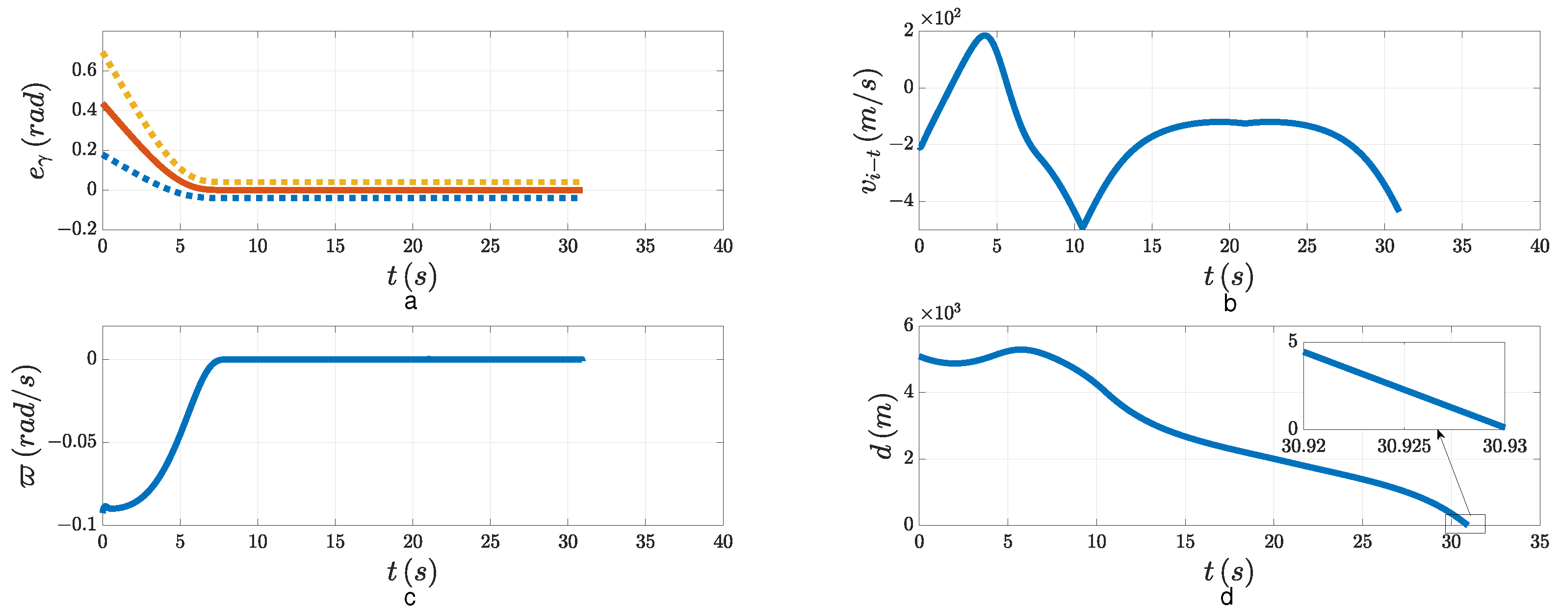From Figure 16a,c, both the tracking error and the LOSAR were stabilized using the FPPC within the specified finite time $T_F$. As can be seen in Figure 14a, the overshoot of the tracking error was small. That means that the smooth change in the LOSA gave the system a good performance. From Figure 16b, the relative velocity was negative when the LOSAR remained in a small enough neighborhood to zero. In Figure 16d, the relative distance finally converged to the minimum distance. 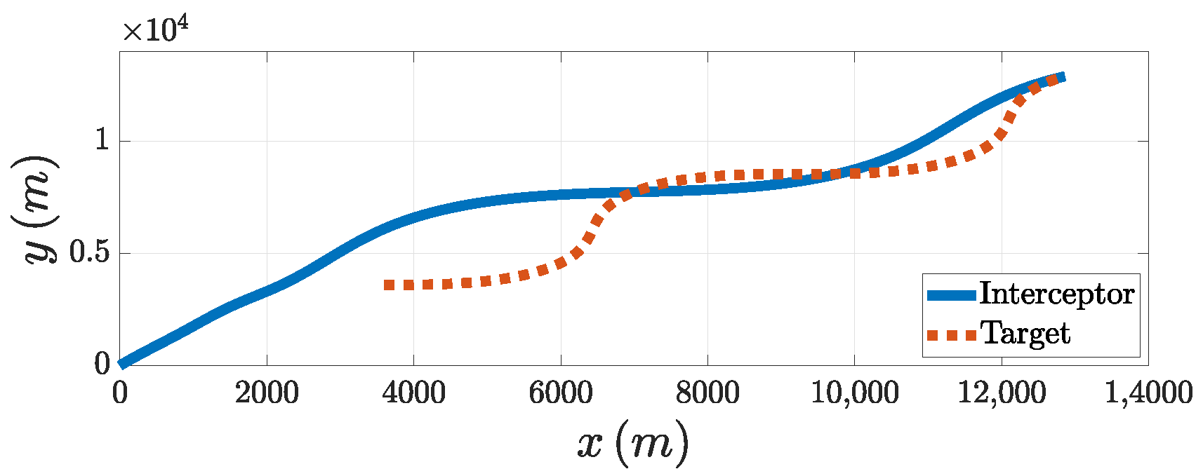The PAG law is shown in Figure 17. In addition, in Figure 18, we can see the trajectories of both the interceptor and the target. Therefore, the effectiveness of the guidance law was illustrated when the target performed a square-like maneuver.

Figure 14. Signals of the interception system without guidance law in Scenario 3: (a) The LOSAR; (b) The relative distance.

Figure 15. The disturbance and its estimation in Scenario 3.

Figure 16. Closed-loop signals of the interception system in Scenario 3: (a) The LOSA error; (b) The relative velocity; (c) The LOSAR; (d) The relative distance.

Figure 17. The interceptor’s acceleration in Scenario 3.

Figure 18. Engagement trajectory in Scenario 3.

In order to illustrate the guidance performance of the PAG law designed in this paper, we used the existing PNG method for a comparative analysis. The PNG law is given as [36]

$$\begin{array}{c}\hfill a_i=-k_{pn}\dot{d}\varpi \end{array}$$

(45)

where $k_{pn}\ge 2$ is the unitless coefficient of PNG. In this section, $k_{pn}=5$. Then, we input the PNG law into the system (5) and compared its guidance performance with the PAG law designed in this paper for Scenario 1, Scenario 2, and Scenario 3. The relative distance with the PNG law (40) is shown in Figure 19.

Figure 19. The relative distance with the PNG law in the three scenarios.

The guidance accuracies of the interceptor with the PNG law (40) and the PAG law designed in this paper in the different scenarios are shown in Table 3.

Through comparing the precision of PNG and PAG in the different scenarios, it was seen that the PAG law designed in this paper had a higher precision in the cases of intercepting the three kinds of target maneuvers. The precision of PNG in the three cases was inferior to that of the PAG. When intercepting a target performing a square wave maneuver, the interceptor even missed the target. Therefore, it is not difficult to see that the PAG law based on the FPPC had a stable accuracy when intercepting large maneuvering targets. This is because the designed DSDO can estimate the target maneuver well, and the FPPC is designed such that the LOSA error can be kept within the preset bounds during the guidance process.

6. Conclusions

In this study, a PAG law for an interceptor using FPPC was proposed. To eliminate the uncertainty of unknown maneuvering target acceleration, a DSDO was developed. Specifically, the estimation accuracy of the DSDO was independent of the relative distance. Then, in order to realize the PAG, the FPPC was used to ensure the LOSAR converged to the neighborhood of zero within the specified finite time and to make it remain at zero during the interception. In this way, the speed of the interception system was also improved. All signals of the interception system could guarantee UUB, and the feasibility of the PAG law is illustrated by the simulation results.