Article

Fast Trajectory Generation with a Deep Neural Network for Hypersonic Entry Flight

1
School of Transportation Science and Engineering, Beihang University, Beijing 100191, China
2
Beijing System Design Institute of the Electro-Mechanic Engineering, Beijing 100074, China
3
Chinese Ordnance Navigation and Control Technology Research Institute, Beijing 100089, China
*
Author to whom correspondence should be addressed.
Aerospace 2023, 10(11), 931; https://doi.org/10.3390/aerospace10110931
Submission received: 4 September 2023 / Revised: 30 October 2023 / Accepted: 30 October 2023 / Published: 31 October 2023
(This article belongs to the Section Aeronautics)

Abstract

:
Optimal entry flight of hypersonic vehicles requires achieving specific mission objectives under complex nonlinear flight dynamics constraints. The challenge lies in rapid generation of optimal or near-optimal flight trajectories with significant changes in the initial flight conditions during entry. Deep Neural Networks (DNNs) have shown the capability to capture the inherent nonlinear mapping between states and optimal actions in complex control problems. This paper focused on comprehensive investigation and evaluation of a DNN-based method for three-dimensional hypersonic entry flight trajectory generation. The network is designed using cross-validation to ensure its performance, enabling it to learn the mapping between flight states and optimal actions. Since the time-consuming training process is conducted offline, the trained neural network can generate a single optimal control command in about 0.5 milliseconds on a PC, facilitating onboard applications. With the advantages in mapping capability and calculating speed of DNNs, this method can rapidly generate control action commands based on real-time flight state information from the DNN model. Simulation results demonstrate that the proposed method maintains a high level of accuracy even in scenarios where the initial flight conditions (including altitude, velocity, and flight path angle) deviate from their nominal values, and it has certain generalization ability.

1. Introduction

In recent years, the application of the new generation of artificial intelligence technologies, represented by Deep Neural Networks (DNNs), has made significant progress across various domains. In 2006, Geoffrey Hinton proposed the concept of deep learning, which introduced a model known as a Deep Belief Network (DBN) [1]. This network consists of multiple stacked Restricted Boltzmann Machines (RBMs) [2]. He developed a pretraining algorithm for rapid training of DBNs, which was the beginning of the third resurgence of artificial intelligence. In 2012, the AlexNet model proposed by Alex and Geoffrey achieved groundbreaking results in image classification [3]. They abandoned the layer-wise greedy training algorithm, opting to directly utilize Graphics Processing Units (GPUs) for training. Since the introduction of the AlexNet model, attention has been drawn to the enormous potential of DNNs in computer vision and language processing.
Meanwhile, researchers have begun to explore the potential applications of deep learning in other fields. The application of deep learning in aerospace guidance, control, and dynamics has yielded some research outcomes [4]. Sánchez, Dario, and others [5,6] have systematically studied DNNs in the context of optimal state feedback control for deterministic, continuous-time, and nonlinear systems, including stability analysis of inverted pendulums, precise landing control for quadcopter aircraft and spacecraft, etc. These systems involve cost functions for smooth continuous or discrete optimal control. The research indicates that DNNs can proficiently accomplish tasks, and even when selecting trajectories beyond the training range, the network’s predictions still meet the requirements effectively. This shows the networks’ inherent robustness. In these studies, the authors pointed out that DNNs were not merely interpolating the control data but might have learned the underlying dynamical relationships within the state and control space of nonlinear systems. Dario and his colleagues [7] extended this research to interplanetary trajectories and investigated how to train DNNs to guide a spacecraft along optimal paths from Earth to Mars. They coined this approach “Guidance and Control Networks” (G&CNETs) [8], which employed DNNs trained through imitation or supervised learning to achieve optimal trajectory prediction. The authors also provided a differential algebra-based method to elucidate its stability margin and control precision. G&CNETs are simple fully connected feedforward neural networks and they illustrated the potential of using relatively straightforward neural networks to replace current onboard navigation and control algorithms. Based on these studies, Furfaro et al. [9] devised a Long Short-Term Memory (LSTM) recurrent neural network to predict the fuel-optimal thrust from a sequence of states during powered planetary descent. They validated the algorithm through Monte Carlo simulation experiments in a lunar landing scenario. Another study by Furfaro et al. [10] utilized Convolutional Neural Networks (CNNs) for excellent image classification performance and applied them to lunar surface image processing. The data from these processes were then fed into LSTMs for spacecraft control during landing, showcasing a comprehensive application of different types of DNNs. While there have been some achievements in employing deep learning for real-time control of spacecraft trajectory landing and orbit transfer [11,12,13,14,15], the research on applying deep learning to real-time optimal trajectory generation for hypersonic vehicles remains relatively scarce.
The real-time onboard generation of optimal trajectories for hypersonic vehicles poses an exceptionally intricate challenge due to the intricate nonlinear flight dynamics constraints of hypersonic flight and the uncertainty stemming from initial flight conditions. In practical scenarios, hypersonic aircraft trajectories require rapid responsiveness and adjustments, which imposes stringent demands on the real-time capability of trajectory control systems. Amidst the amalgamation of these factors, it is essential to ensure robustness, rapidity, and guidance accuracy in the application of onboard systems. Thus, the development of efficient online trajectory optimization algorithms capable of fulfilling the demands of complex hypersonic flight missions is an urgent imperative.
One main approach to enhance the performance of online trajectory generation for hypersonic entry flight is the convex optimization technique. Wang et al. [16] formulated the highly nonlinear problem of planetary-entry optimal control as a series of convex problems and employed an interior-point method to solve these convex optimization problems. The results demonstrated that this solving method converges to the exact solution faster than general-purpose solvers. Wang [17] further improved the algorithm by introducing line-search and trust-region techniques, fundamentally enhancing the performance of sequential convex programming methods in ballistic trajectory optimization. However, the high computational cost and convergence issues to some extent hinder its onboard application in hypersonic trajectory optimization [18,19].
To explore more effective solving methods, researchers have started to experiment with emerging technologies such as artificial intelligence and machine learning. In the field of deep reinforcement learning, Gao et al. [20] optimized the reentry phase of a Reusable Launch Vehicle (RLV) using a deep reinforcement learning method and validated the feasibility of the Deep Deterministic Policy Gradient (DDPG) algorithm for continuous nonlinear optimization problems through comparisons with the Particle Swarm Optimization (PSO) algorithm. Wu [21] employed a deep reinforcement learning approach to address the design problem of feedback gains in the entry guidance of hypersonic vehicles. By comparing the results of Monte Carlo simulation, the algorithm achieved real-time adjustment of feedback gains within a certain error range. Solari [22] investigates the Powered Descent (PD) phase of Mars landings using a reinforcement learning approach with a policy model based on Neural Networks (NNs) with only one hidden layer. The results demonstrate that this algorithm architecture exhibits robustness against disturbances and generalizes effectively to regions of the state space beyond the training domain.
In the deep learning domain, which is the focus of this paper, Yang et al. [18] following the research methodology of G&CNETs, extending this approach to generating optimal trajectories for a hypersonic vehicle. Simulation results demonstrated that their designed network exhibited favorable control accuracy and robustness. However, their consideration was limited to the two-dimensional longitudinal plane motion trajectory of the hypersonic entry, involving relatively fewer flight states and control variables. Wang et al. [19] extended Yang’s work to address three-dimensional optimal trajectory planning for hypersonic entry vehicles. They also incorporated terminal states into their training dataset to ensure the generation of trajectories under varying terminal conditions. However, their simulation results indicated that the accuracy in the predicted trajectories of the network model needs to be improved. Due to the absence of the initial flight state range and visually intuitive trajectory fitting curves in simulations, it is hard to validate the robustness of the trajectory generated by the network. Wang et al. [23], capitalizing on the advantages of deep learning in neural network mapping and real-time performance, utilized the real-time state information of entry vehicles. They employed LSTM models to generate real-time bank angle commands, enhancing computational efficiency while ensuring guidance precision. Cheng et al. [24] combined DNNs with constraint management techniques, proposing an intelligent multi-constraint prediction–correction guidance algorithm. Simulation results demonstrated the algorithm’s ability to achieve trajectory corrections at a 20 Hz update rate, offering accurate entry guidance for hypersonic flight.
The primary approach in the aforementioned studies is to generate multiple high-precision optimal trajectories using either a direct or indirect method. The optimal state–action sets from these trajectories are then employed as training inputs for the network, with the network outputting optimal control commands for the flight. The network is subjected to offline training. Subsequently, the trained network is integrated into the guidance system to serve as a controller, enabling real-time generation of optimal guidance control commands. In summary, while these studies have yielded promising results for specific problems, they lack comprehensive analyses of sample data reliability, network architecture, and parameter design. In this paper, a simulation verification of the trajectories in the sample database obtained via GPOPS is described based on a 3 Degrees of Freedom (3Dof) flight dynamics model of a hypersonic vehicle. This ensured the reliability of the trajectory data used for network training and testing. Furthermore, the network’s architecture and parameters were determined through cross-validation, and callback functions were introduced to optimize the network, ensuring its excellence in the study case. These efforts effectively enhanced the accuracy and generalization capability of network predictions.
This paper provides an in-depth, comprehensive examination and assessment of the DNN-based generation method for three-dimensional optimal trajectories of hypersonic vehicle entry. Firstly, using the pseudo-spectral method and algorithm package GPOPS II [25], the optimal flight trajectories of the hypersonic vehicle entry flight are generated. The state–action sets are then extracted from these trajectories and used as training samples for the network model after simulation checking. Verification experiments are designed to ensure the authenticity of the data sample library. Subsequently, the network architecture and hyperparameters are designed and analyzed. The network model is trained offline to effectively learn the underlying mathematical relationships within the hypersonic vehicle’s optimal flight state–action set. This allows the network model to predict optimal control and trajectories. Finally, nonlinear simulations based on the 3Dof flight dynamics model are conducted. Numerical analysis of prediction errors is performed to validate the feasibility of the algorithm and assess its robustness under some uncertain conditions. In this study, the most time-consuming and computationally intensive training process is conducted offline. The trained network solely requires straightforward matrix addition and multiplication operations within its hidden nodes based on the input state set to generate the requisite optimal control commands. Consequently, this algorithm can achieve the generation of the optimal trajectory of the hypersonic vehicle while ensuring expedited execution. The contributions of this paper are mainly in two aspects. Firstly, a detailed analysis of the impact of network structure and parameters on prediction results is conducted. The network model is designed using cross-validation to ensure its quality, effectively enhancing the guidance accuracy of the network. Secondly, the performance of the network and its adaptability to varying initial flight states is evaluated through multiple sets of 3Dof nonlinear simulation experiments. By comparing with numerical optimization methods, the paper demonstrates that the network exhibits significant accuracy and robustness.
The structure of this paper is as follows. In Section 2, the continuous-time optimal control problem of three-dimensional hypersonic entry flight is presented. Using the GPOPS II package, a large amount of flight trajectories are generated, which serve as training and test samples for the network. In Section 3, the detailed network design process is given, and the predictive results of the model are analyzed. Section 4 conducts simulation experiments on the trained network model, followed by a numerical analysis of errors. This section evaluates the performance of the trajectory generation method based on the network model.

2. Problem Formulation

2.1. Problem Statement

This section primarily introduces the investigated optimal trajectory planning problem of a hypersonic vehicle entry flight, which is selected from reference [26]. The optimal objective is to choose a set of control variables to maximize the cross-range, which is one of the important issues in determining the footprint for high-speed entry flight. It somehow indicates the flight scope covered by a hypersonic entry vehicle. The objective is defined as maximizing the terminal latitude.
J = ϕ ( t f )
The 3Dof flight dynamics model for hypersonic vehicles is given as follows:
d r d t = v sin γ
d θ d t = v cos γ sin ψ r cos ϕ
d ϕ d t = v cos γ cos ψ r
d v d t = F d m g sin γ
d γ d t = F l cos σ m v g v v r cos γ
d ψ d t = F l sin σ m v cos γ + v cos γ sin ψ tan ϕ r
r represents the radial distance of the aircraft from the Earth’s center. θ stands for longitude. ϕ denotes latitude. v is the relative velocity of the aircraft with respect to the Earth. γ represents the flight path angle. ψ is the heading angle. F d , g , F l , σ respectively denote drag, gravitational acceleration, lift, and bank angle. m denotes the mass of the vehicle. The flight state vector x is represented by [ r , θ , ϕ , v , γ , ψ ].
Lift and drag are functions of altitude, velocity, and angle of attack:
F l = 1 2 S r e f ρ v 2 c L ( α )
F d = 1 2 S r e f ρ v 2 c D ( α )
S r e f is the aerodynamic reference area. ρ is the atmospheric density. C L and C D are the lift and drag coefficients, respectively. The control vector u is represented by [ α , σ ] where α is the angle of attack.
The final point of the entry trajectory occurs at an unknown (free) time t f . As the design objective is to maximize cross-range, terminal constraints do not impose limitations on the terminal values of longitude and latitude. The hypersonic entry flight is one of flight phases of the whole flight mission and is not the last flight phase. So, the final altitude is not zero (about 24,384 m), and the final fight path angle and velocity are constrained to specific values. Table 1 presents the boundary conditions for the nominal flight trajectory.
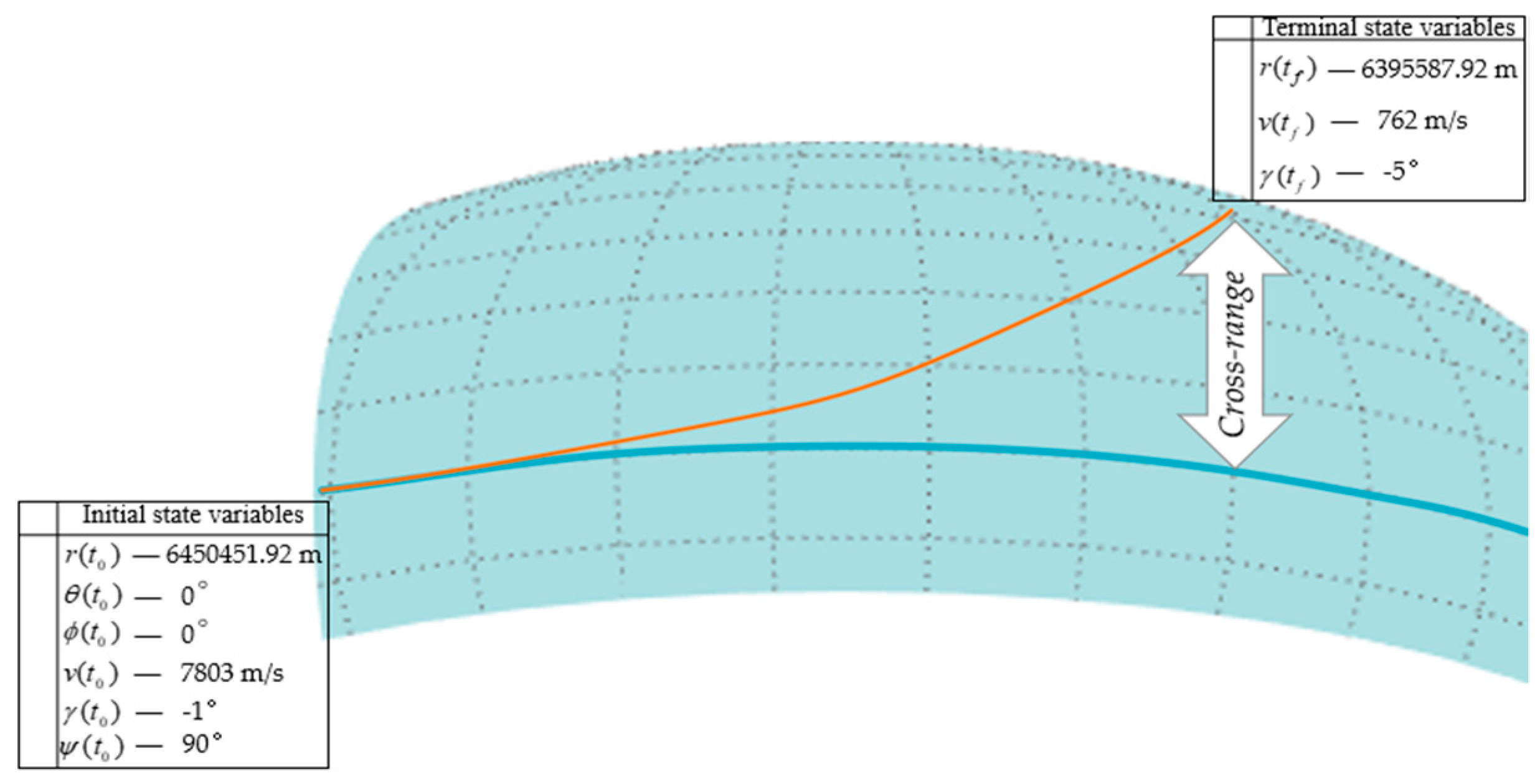
Figure 1 illustrates this optimal entry trajectory problem of the hypersonic vehicle, along with the initial and terminal boundary conditions for the vehicle’s flight.
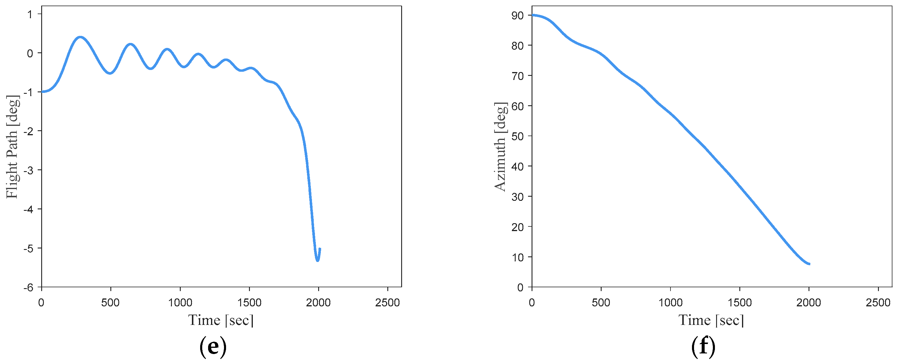
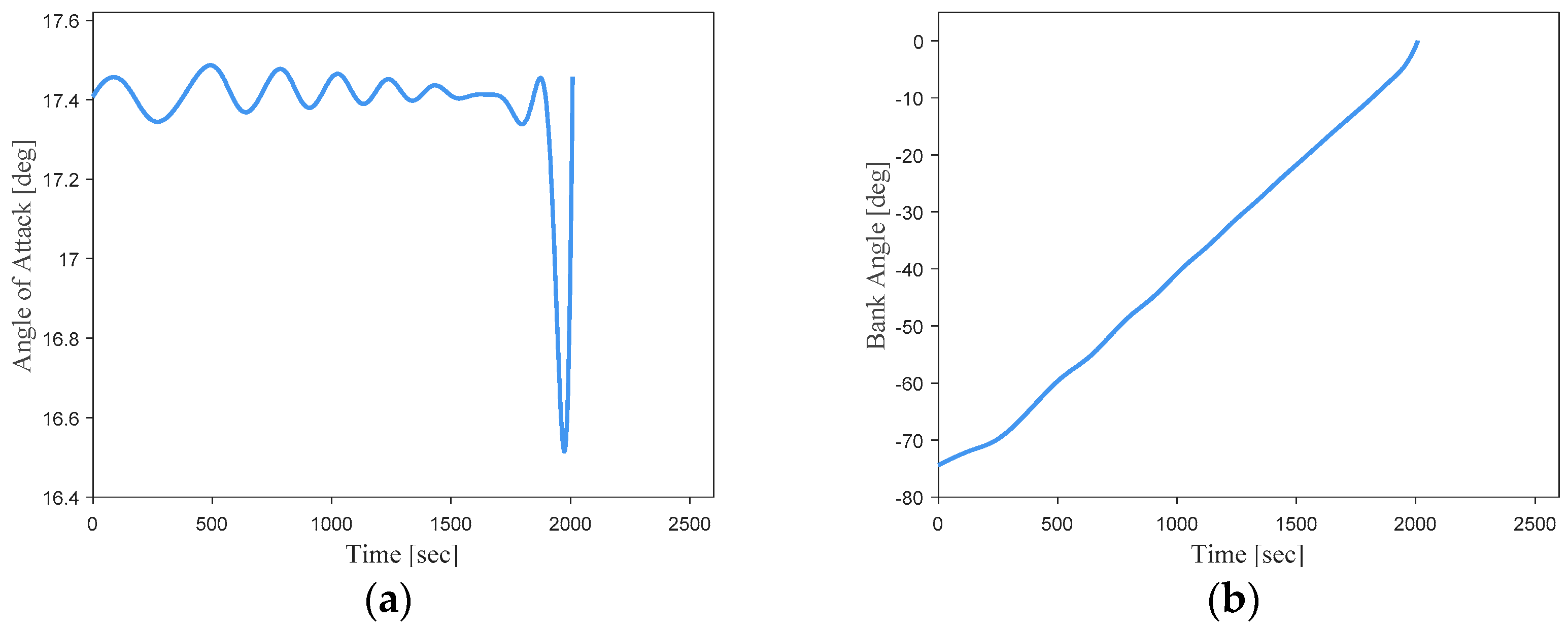
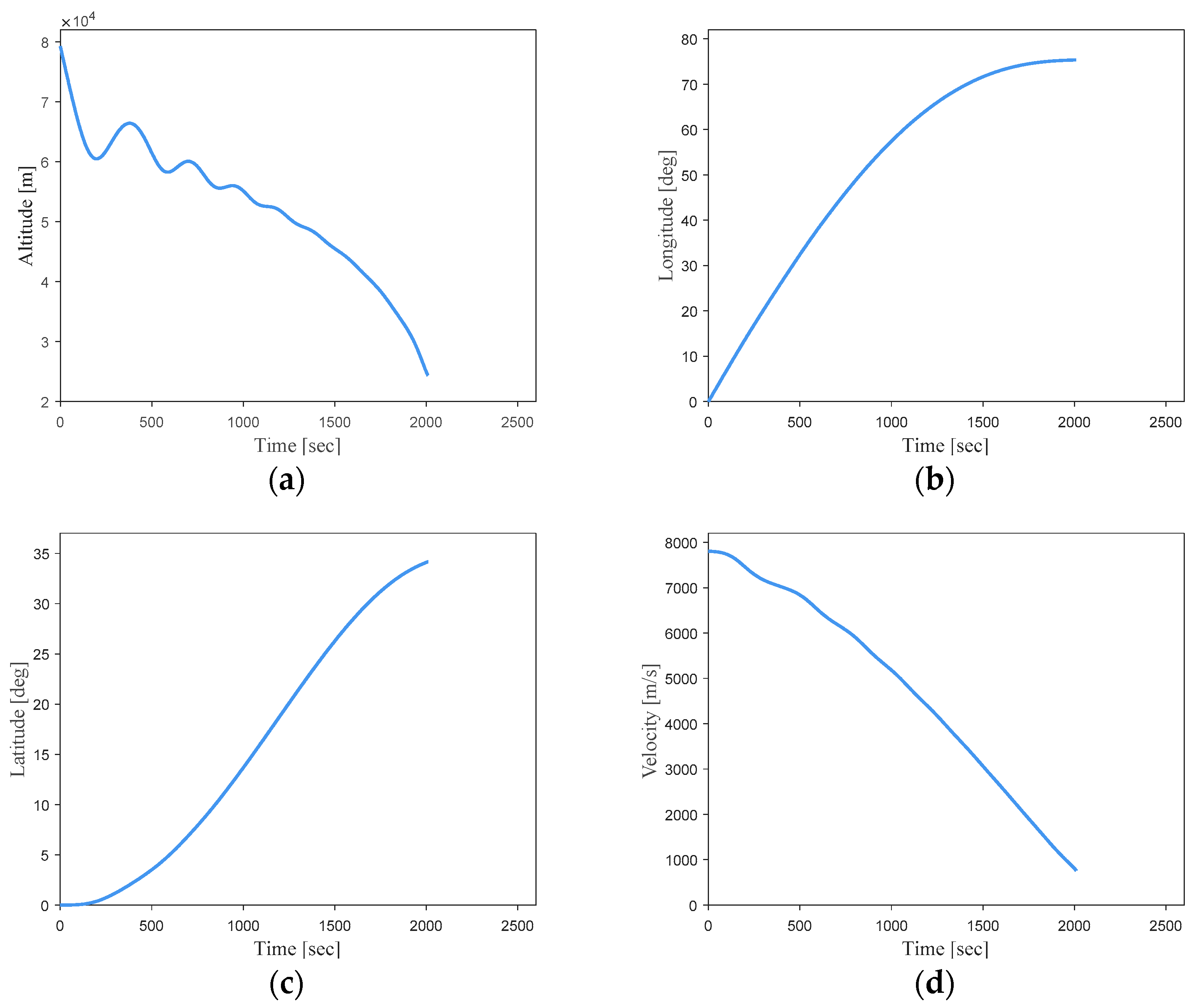
Figure 2 and Figure 3 depict the optimal trajectory generated using the direct method (GPOPS II) under nominal entry initial flight condition. Remarkable nonlinear relationship between flight states (velocity, flight path angle, etc.) and optimal control inputs (angle of attack and bank angle) can be observed. The DNN-based guidance controller is designed and used to capture the inherent nonlinear mapping between states and optimal actions. It is worth noting that the trajectory sample database employed for subsequent network training was generated by varying the flight initial conditions.

2.2. Generation of Training and Test Data

Considering the requirements of hypersonic vehicle entry flight missions, their initial flight states might be variable. It is crucial to ensure that even when the initial state deviates from the nominal values, the vehicle can still generate optimal or near-optimal trajectory to guide it through the mission. To enable the DNN, serving as a trajectory generator, to adapt to a wide range of initial conditions, a substantial number of optimal trajectories with various initial flight states are chosen as the training datasets. This ensures that the neural network can learn the underlying mapping relationships between flight states x (including [ r , θ , ϕ , v , γ , ψ ]) and optimal control actions u .The optimal control variables refer to the angle of attack α and bank angle σ .
In this paper, the Gaussian pseudo-spectral method tool, GPOPS II, is applied for generating an optimal trajectory library. One of the key influencing factors in numerically generating optimal trajectories is the number of Gaussian collocation points on each trajectory. Too few collocation points compromise the quality of trajectory optimization, while too many collocation points increase the time cost of both trajectory generation and subsequent network training significantly. For the specific case considered in this study, we find that an average time interval of about 1 s between two collocation points can generate trajectories with enough accuracy. The entry flight time would be about 1000–2000 s. After trading off between trajectory generation time and trajectory optimization quality, it was determined that each trajectory should have an average of around 1600 discrete optimal state–action sets. This design allowed us to generate reliable flight trajectories within acceptable time costs. It is worth mentioning that using even more Gaussian collocation points is feasible, but it would come at a significant time cost. The current selection of discretization points already ensures the reliability of the trajectories, and a detailed analysis regarding trajectory reliability is presented below. Within the initial state value range as shown in Table 2, a total of 6261 trajectories were optimized. These trajectories include approximately 10,000,000 data points, which are used as training samples for the neural network. The scale of this sample database is determined by referencing relevant literature [18,19,24] and ensuring that the network can learn from a wide range of potential flight scenarios in the given case. These samples are divided into training and validation sets with a ratio of 90/10.
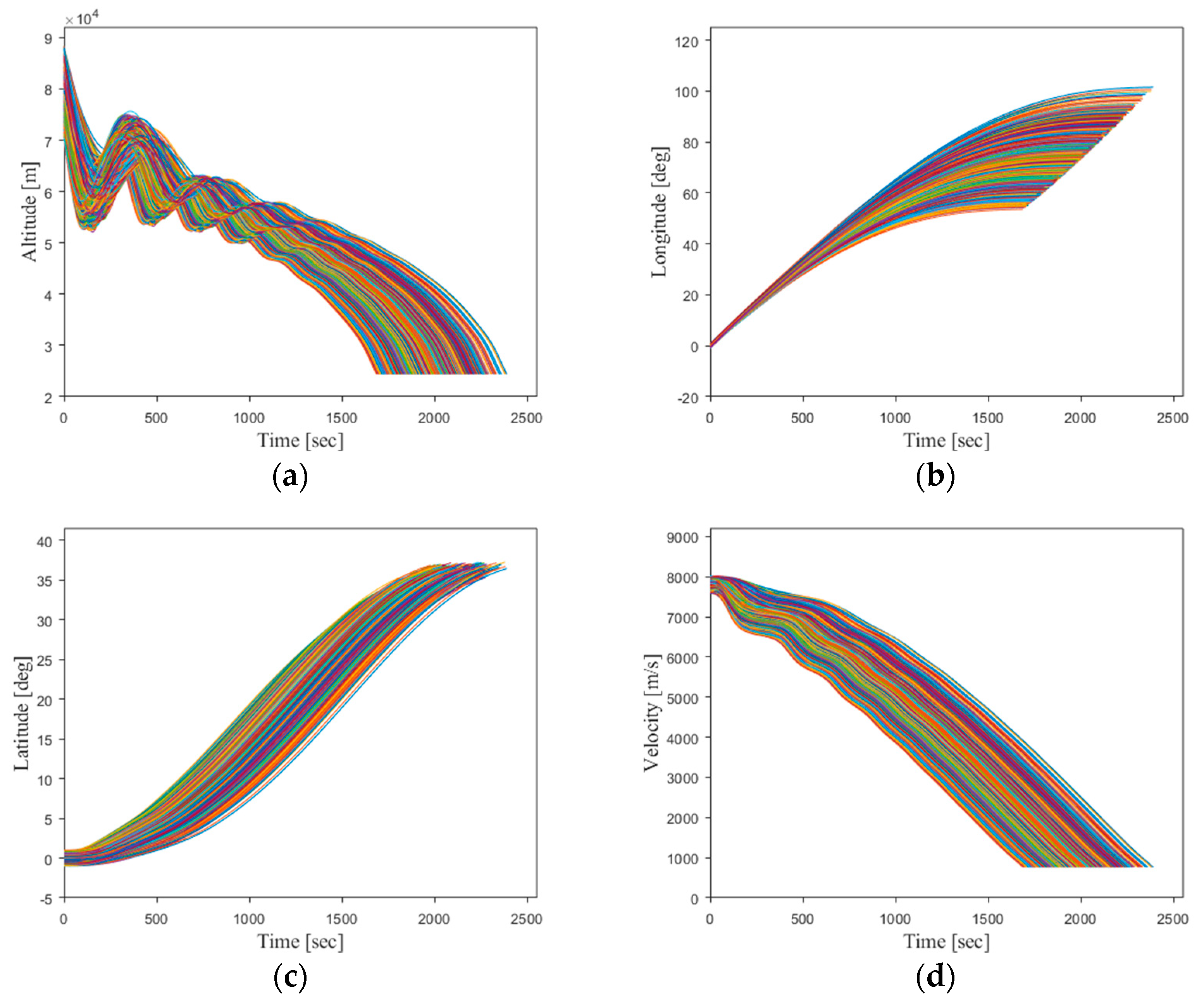
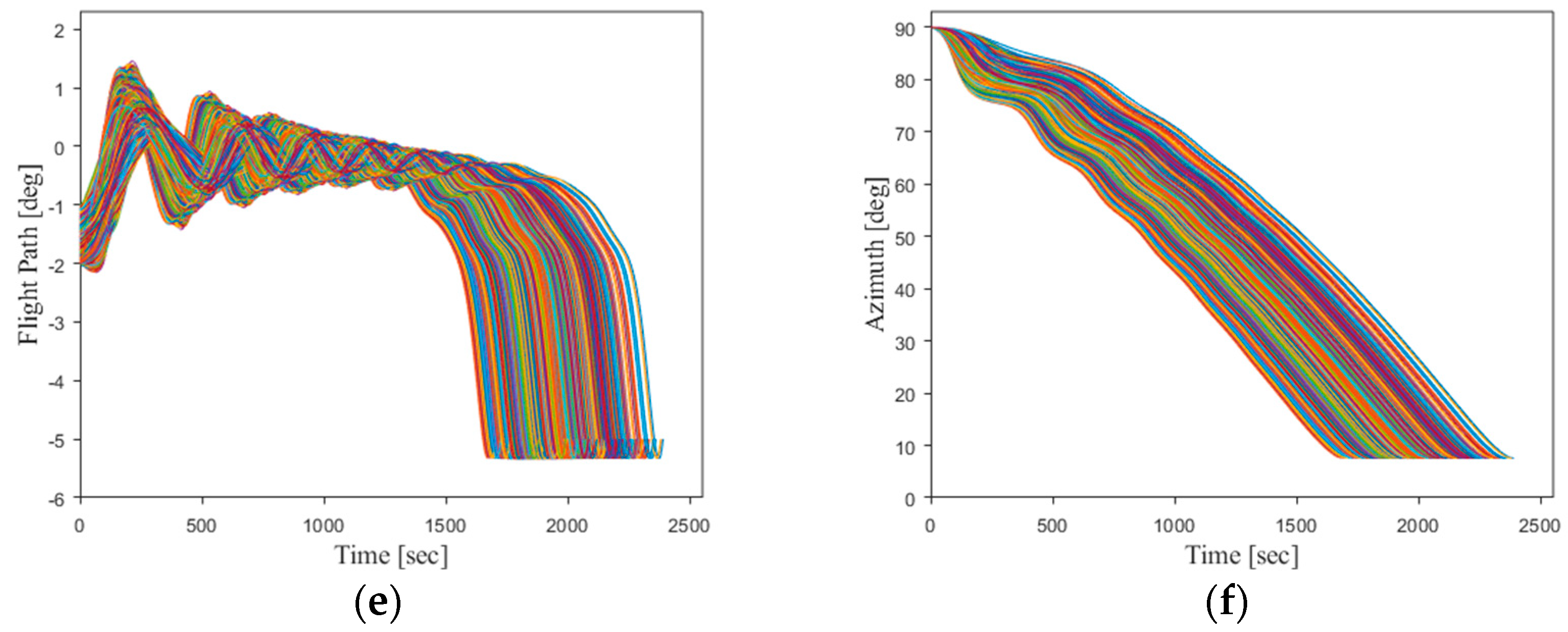
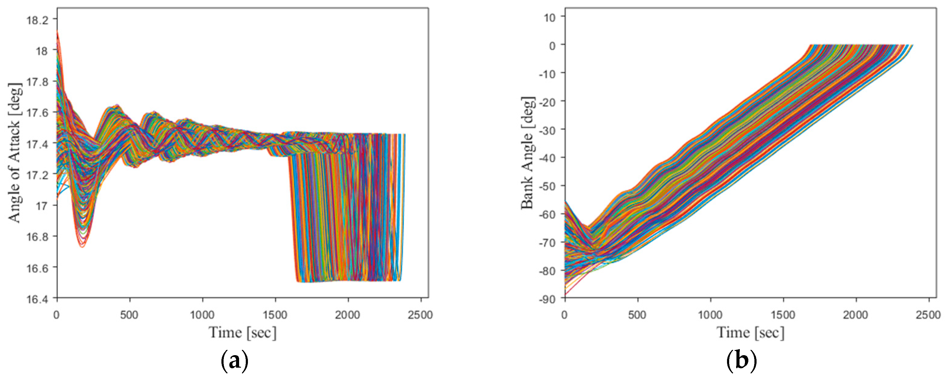
Figure 4 and Figure 5 depict the 6261 optimal trajectories randomly generated within the aforementioned range of initial values for altitude, longitude, latitude, velocity, and flight path angle.
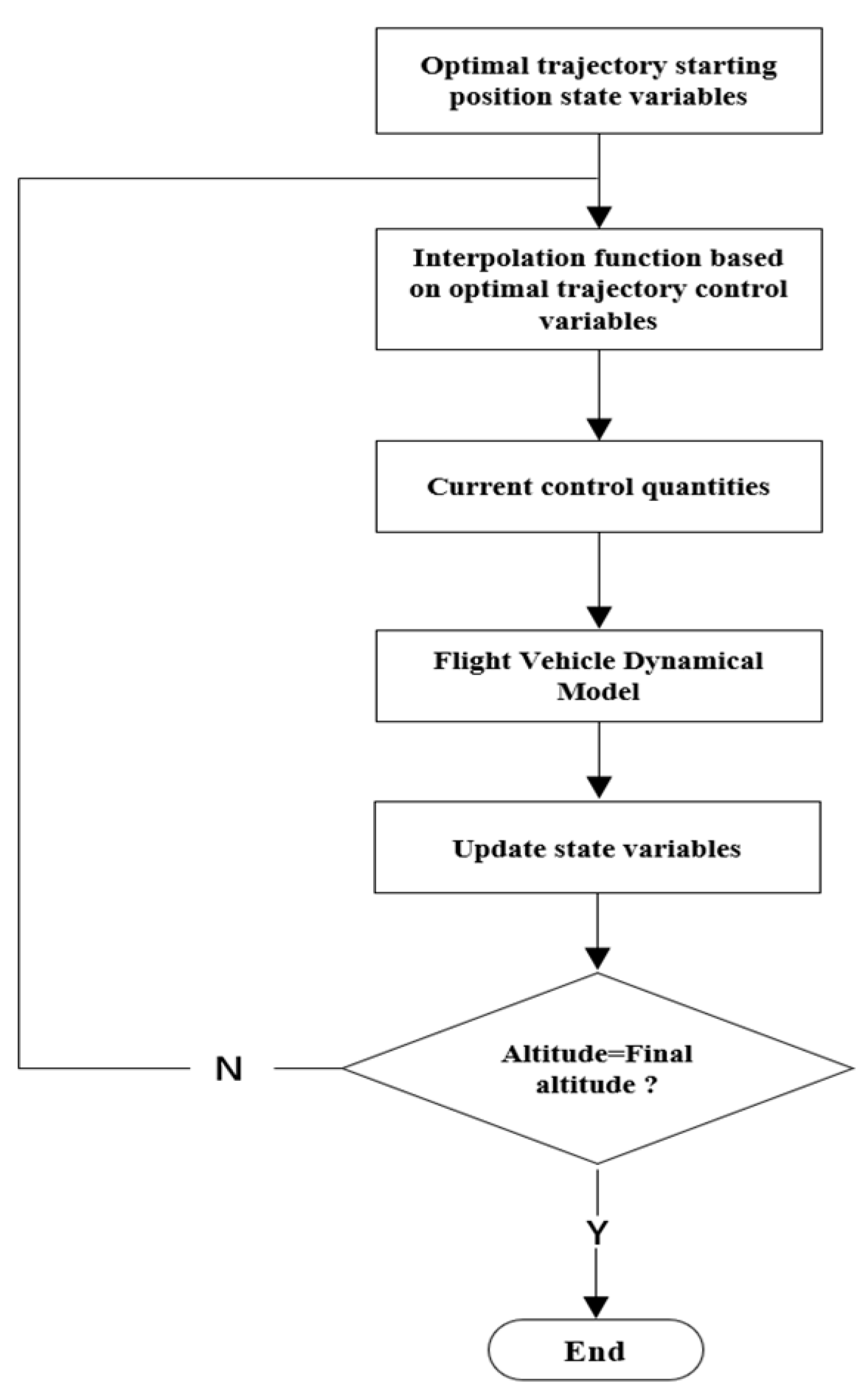
To validate the quality of numerical optimal trajectories, all generated sample data underwent simulation verification based on the 3Dof flight dynamics. The computational process is illustrated in Figure 6.
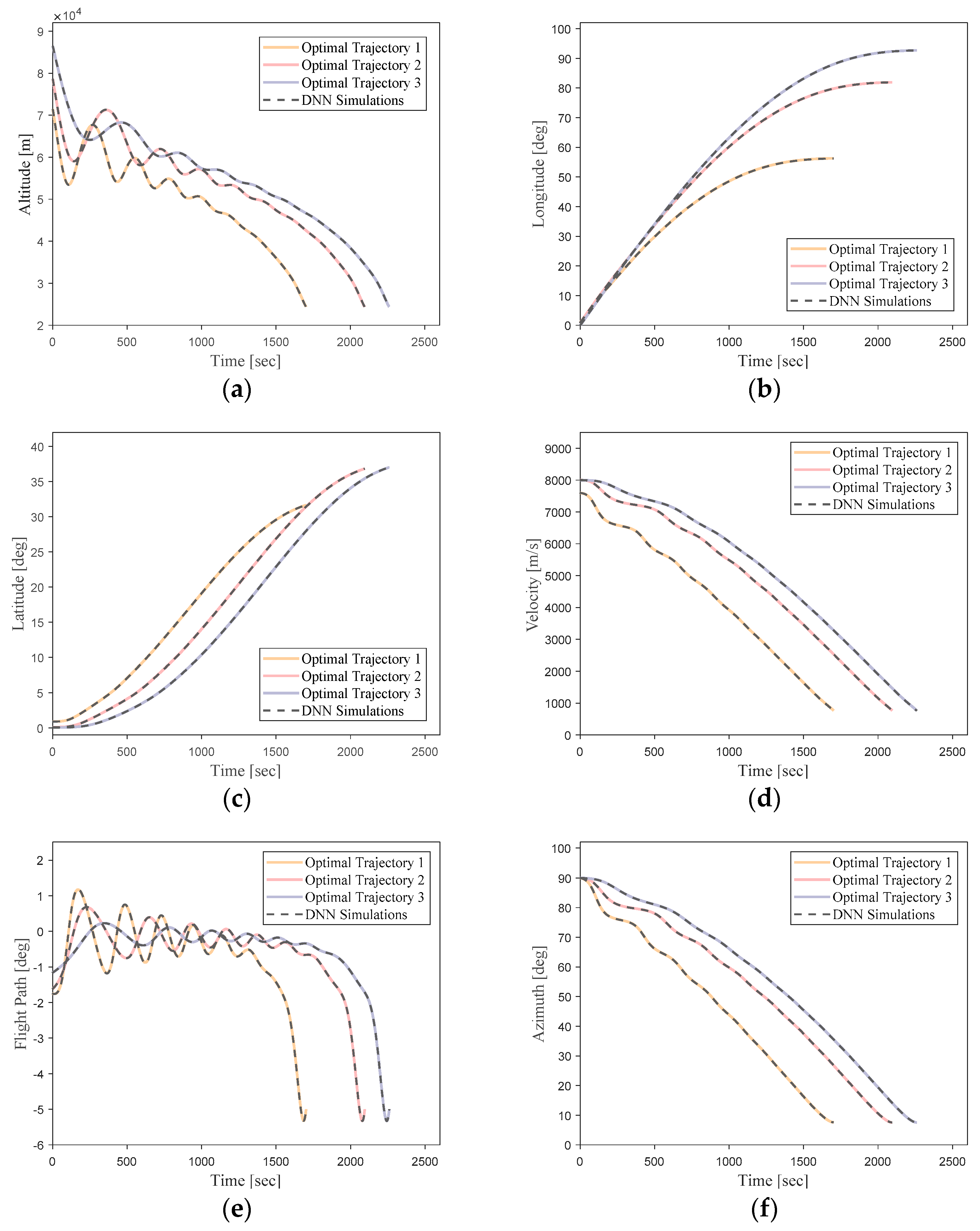
In this computational process, we input the initial flight state x of the optimal trajectory along with the optimal control u –time profiles. By interpolating the angle of attack–time profiles and bank angle–time profiles, we obtain the optimal flight control quantities at each step time. Subsequently, these data are substituted into Equations (2)–(7) to calculate the flight state at the next step. This process repeats iteratively until the flight altitude descends to the final altitude, concluding the computation. Table 3 presents the absolute errors from our simulation calculations for all flight trajectories within the optimal trajectory library.
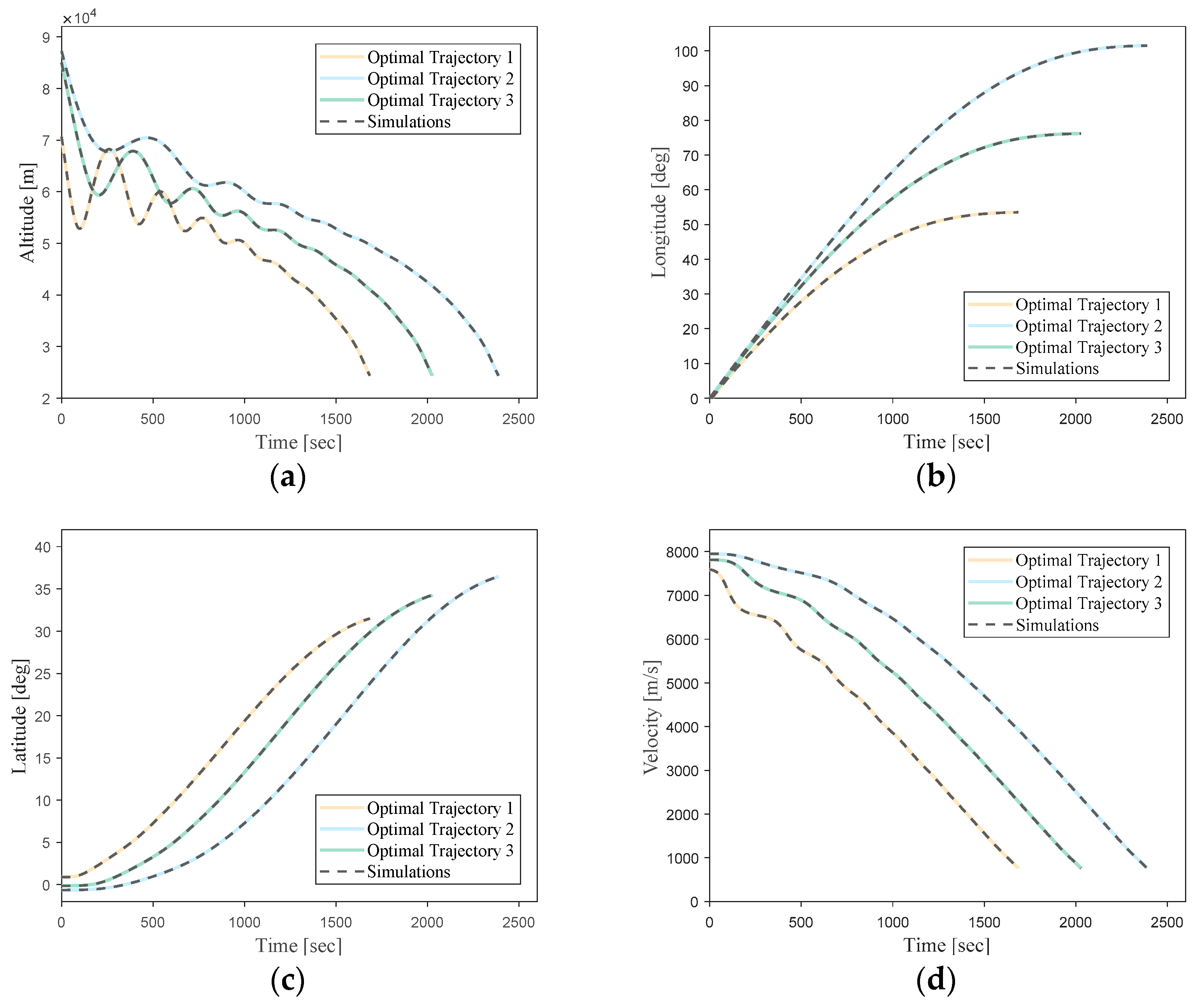
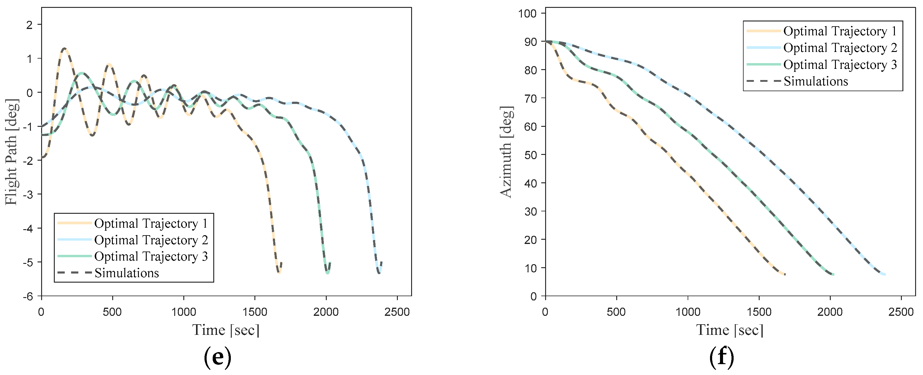
To provide a more visual representation of the simulation results, three trajectories were randomly selected, as shown in Figure 7. The results indicate that the optimal trajectory sample data used for network training possess high-fidelity optimization quality. It is noteworthy that the subsequent training and validation data of optimal trajectories have all undergone simulation verification to ensure their accuracy.

3. DNN-Based Fast Trajectory Optimization

Neural networks can learn the nonlinear mathematical relationship between input state vectors and optimal control outputs. The trained neural networks would serve as the controller in the onboard guidance system to generate guidance commands. Since both the input of sample data and network training are conducted offline, the DNN-based optimal trajectory optimization algorithm is expected to significantly reduce the time required for online control command generation while ensuring precision.

3.1. Overall Design Scheme

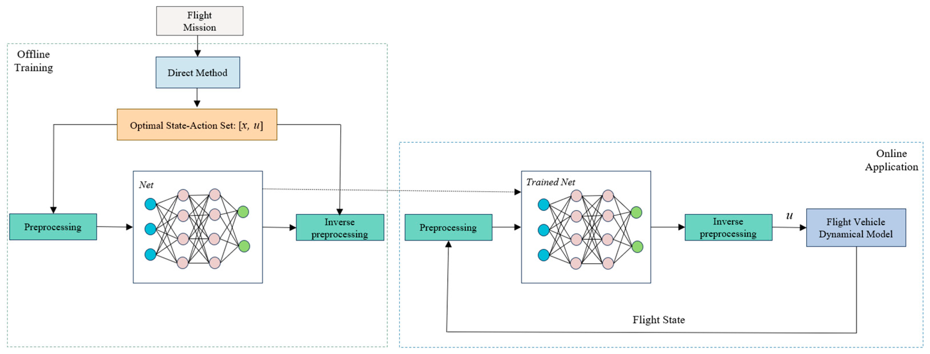
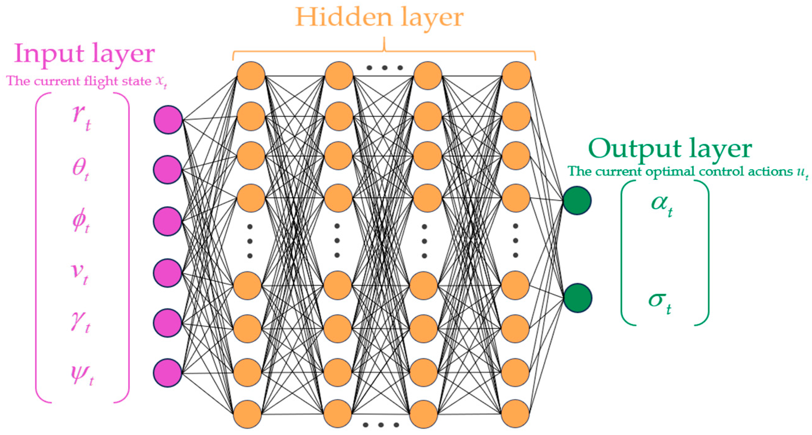
The optimal trajectory generation method for hypersonic entry vehicles based on DNNs is illustrated in Figure 8. In the context of a given flight mission, the optimal state–action dataset is obtained through a direct method. After preprocessing the dataset, it is input into the neural network for offline training. The neural network model can learn the nonlinear mapping relationship present in the dataset. This allows it to predict the optimal control actions of the vehicle based on the flight state feedback. The trained neural network only requires simple multiplication and addition operations on the input current flight state x t to predict the corresponding optimal control actions u t , which are angle of attack α t and bank angle σ t . It is worth noting that these DNN-based guidance controllers have two application scenarios. One involves a trained DNN-based controller capable of directly generating optimal guidance commands based on the current flight state feedback in a real-time manner (usually in milliseconds). The other application scenario is to utilize the DNN-based controller to generate a whole reference entry flight trajectory based on a specific initial entry flight condition in a short time (usually in seconds). The schematic diagram of the online application of DNNs, including its inputs, outputs, and structure, is illustrated in Figure 9.

3.2. Design and Optimization of DNN

This subsection provides details of the design of the network model and the process of hyperparameter selecting. The network model designed in this paper is a fully connected feedforward neural network, consisting of an input layer, several hidden layers, and an output layer. The network’s input consists of the state variables of the optimal trajectory x = [ r , θ , ϕ , v , γ , ψ ], and the neural network learns the underlying nonlinear mathematical mapping relationship between the state vector and the optimal control actions u = [ α , σ ] through training. The output of the i unit in the j layer of the network, denoted as o i j , can be represented as follows:
o i j = g ( w i j o i 1 + b i j )
w i j is the weight vector, b i j is the bias vector for that unit, o i 1 is the full output from the previous layer, and g is the nonlinear activation function of that unit.
By comparing commonly used nonlinear activation functions, it was observed that the Rectified Linear Unit (ReLU) [27] performed the most optimally in this particular case. Consequently, ReLU was employed as the nonlinear activation function in the hidden layers of the network to assist in capturing complex patterns within the data.
Regarding the input state vector, the units for altitude and velocity are m and m/s, respectively. The magnitudes of their values are much larger than those of other state variables. To enhance optimization algorithm performance, expedite convergence, and decrease computational costs, preprocessing is conducted on the altitude and velocity within the input vector. The process is illustrated as follows:
r p r e = r R e , v p r e = v v t 0
where R e signifies the Earth’s radius, v ( t 0 ) is the entry initial flight velocity of the vehicle, r p r e and v p r e represent altitude and velocity after preprocessing, respectively.
In deep learning, a loss function L is used to quantify the difference between the model’s predicted results and the actual labels. It guides and optimizes model training, aiming to minimize this loss function to improve the accuracy of predictions. In this paper, the Mean Absolute Error (MAE) is chosen as the model’s loss function due to its higher robustness. It is defined by Equation (12):
L = 1 N i = 1 N N e t ( x i ) y i
where N is the number of training samples, N e t ( x i ) represents the predicted output of the neural network under the input state vector, and y i represents the optimization data obtained through the direct method.
The first set of hyperparameters to be determined is the network structure, which includes the number of hidden layers and the number of units in each hidden layer. Too few hidden layers or neurons may result in the network struggling to learn the nonlinear mapping relationship between inputs and outputs, which leads to underfitting. On the other hand, too many hidden layers or units can increase training time and risk overfitting, where the network overly learns from the training dataset and performs poorly on the validation set.
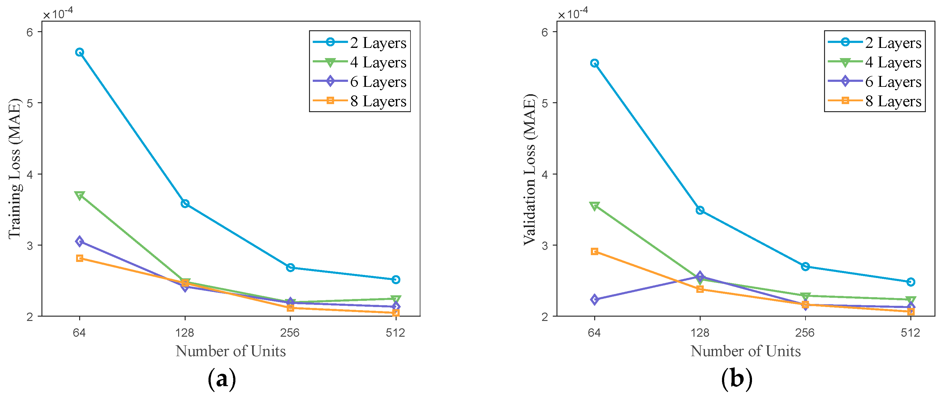
The number of hidden layers and neurons per layer are determined via cross-validation. Various combinations of hidden layer depths and neuron counts are compared by evaluating the loss on both the training and validation sets, as depicted in Figure 10.
The comparative results indicate that networks with fewer layers are insufficient to capture all the features of the samples and achieve the desired accuracy. Networks with more hidden layers generally outperform shallower ones. Moreover, both training and validation set losses decrease as the number of units increases, with no observable overfitting. The final determined network structure consists of 8 layers, each containing 512 units.
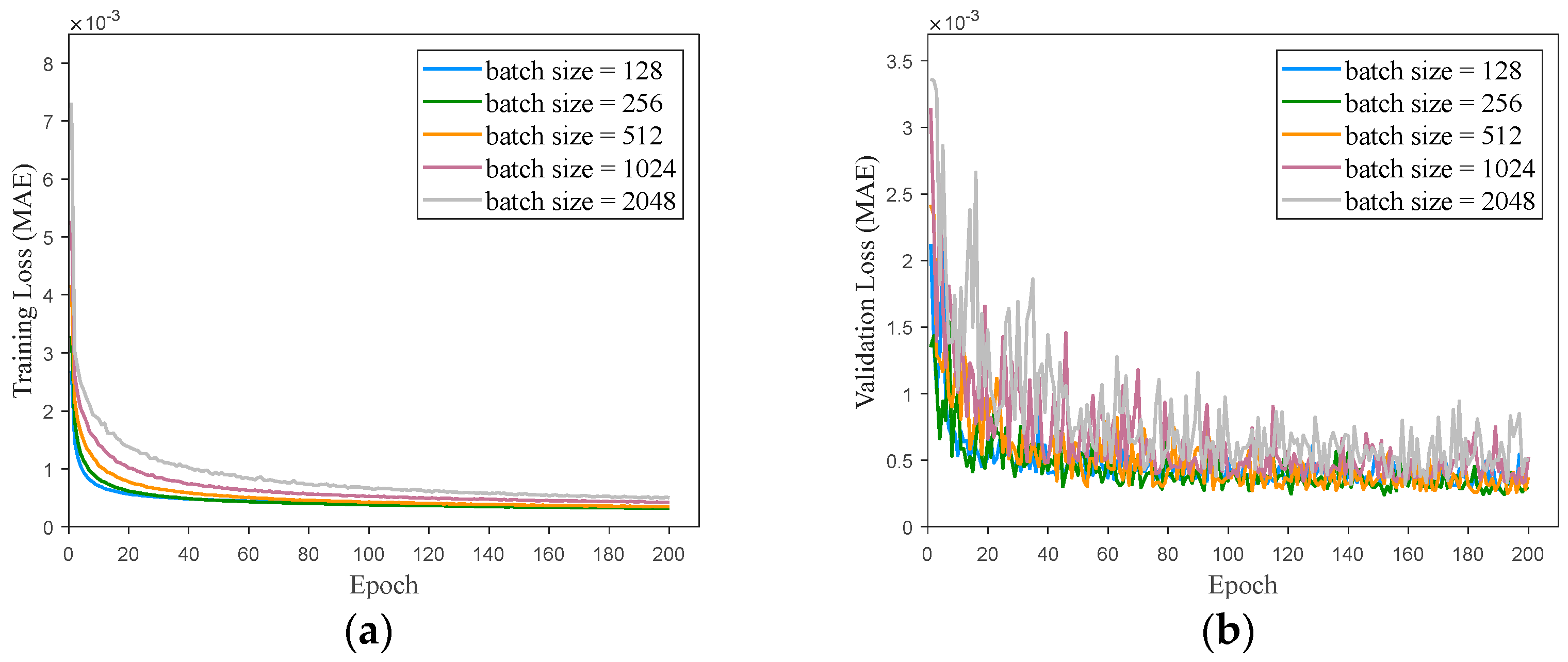
The model weights are updated using the mini-batch gradient descent method. Therefore, another set of hyperparameters to be selected includes batch size and initial learning rate. The batch size parameter specifies the number of samples used in each training iteration. A well-suited batch size allows for the efficient utilization of computational resources, expedites the model training process, and offers more stable gradient estimates. Figure 11 displays the MAE of the network model on the training and validation sets across different batch sizes.
It can be seen that as the batch size increases, the model’s convergence slows down, and oscillations in the validation set become more pronounced. However, a small batch size can significantly extend the model’s training time. This study sets the batch size to 256 in the model design.
Based on mini-batch gradient descent, this paper further introduces the Adam optimization algorithm [28] to enhance the model’s training process. Through its adaptive learning rate feature, the Adam algorithm updates the model’s weight and bias parameters to improve convergence speed and generalization capabilities. The update rule for model parameters Z using the Adam optimization algorithm at time t is as follows:
n t = β 1 n t 1 + ( 1 β 1 ) L Z υ t = β 2 υ t 1 + ( 1 β 2 ) 2 L Z 2 Z t = Z t 1 l t n t υ t + ε
where n and υ represent mean and variance, respectively. The introduction of m is derived from the momentum gradient descent algorithm, which employs historical gradient information to adjust the current gradient, thereby mitigating oscillations during variable updates and achieving more stable gradient updates. The utilization of υ is inspired by the adaptive learning rate gradient descent algorithm. The learning rates l and υ t + ε are treated as a unified entity, resulting in adaptive learning rates. β 1 and β 2 are the forgetting factors, while L is the loss function, and Z denotes the parameters to be updated, encompassing weights w and biases b . ε is a minor constant incorporated to prevent division by zero.
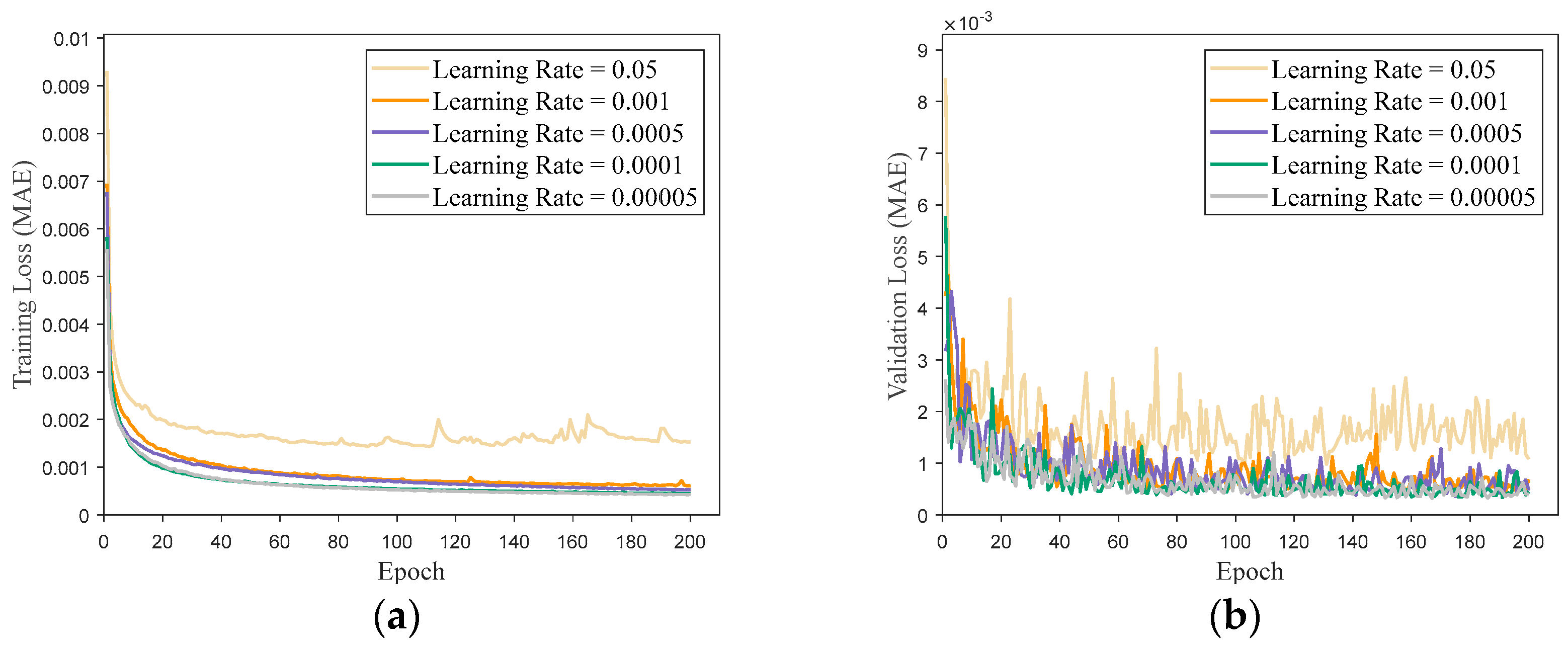
The learning rate controls the step size or speed of each parameter update and determines the magnitude of parameter adjustments during the training process. It plays a crucial role in influencing the convergence speed and performance of the model. A lower learning rate might lead to slow parameter updates and prolonged training times, whereas a higher learning rate could cause the model to converge rapidly towards suboptimal solutions. Selecting an appropriate learning rate is a significant challenge in the model training process. Experiments involving various initial learning rate values are carried out. Results are depicted in Figure 12. Additionally, it is noteworthy that a dynamic learning rate scheduling strategy is also employed to enhance the model’s performance.
From Figure 12, it can be seen that a higher learning rate prevents the model from converging to the optimal solution, while a lower learning rate helps mitigate oscillations. Ultimately, the initial learning rate value is chosen to be 1 ×10⁻⁴.
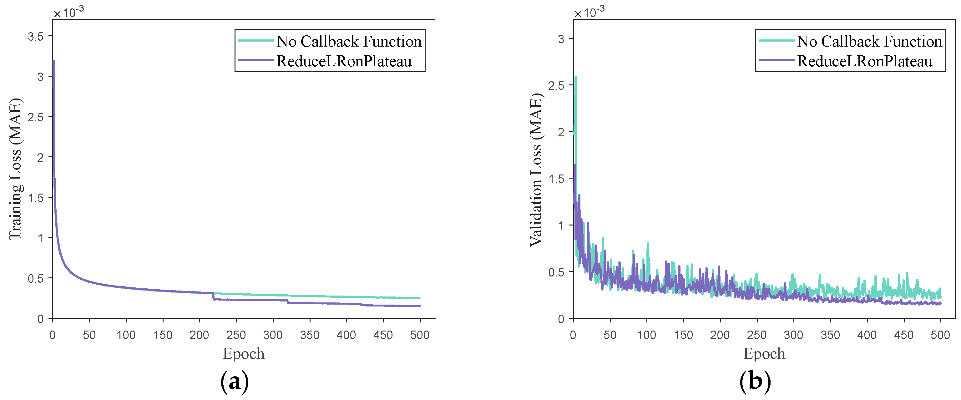
Extensive practical experiences indicate that when a model encounters performance stagnation during training, reducing the learning rate by a factor of 2–10 can help the model escape local minima and optimize more effectively [29,30]. Thus, the ReduceLRonPlateau callback function from the Keras deep learning framework is introduced. This function dynamically adjusts the learning rate during training based on the model’s performance. It monitors the loss metric on the validation set and reduces the learning rate when the metric does not exhibit significant improvement over a specified number of epochs. Figure 13 illustrates a comparison with and without the ReduceLRonPlateau process. As shown, the introduction of the ReduceLRonPlateau allows the model to break out of local optima during training, effectively enhancing the model’s performance and stability.
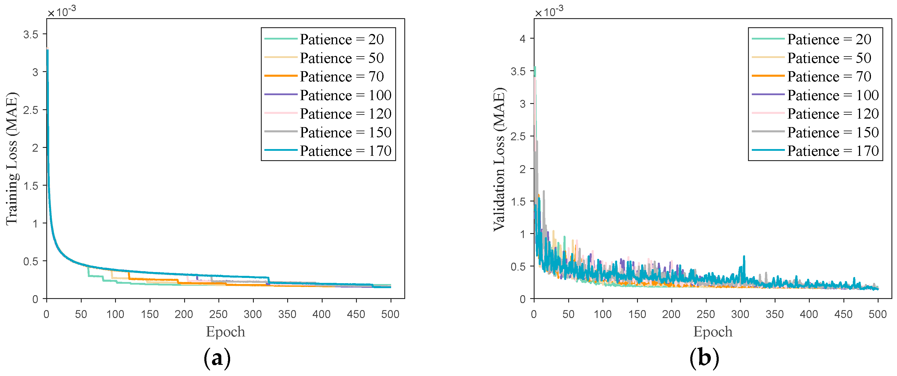
Figure 14 illustrates the impact of different patience levels on model training. Setting various patience levels causes the model to exhibit improvements at different stages, yet all converge to the optimal solution. It does not affect the final network training outcomes significantly. Ultimately, the chosen patience for the callback function is set to 170.

4. Simulations and Result Analysis

In this section, the effectiveness of the DNN-based optimal trajectory generation algorithm is evaluated through simulation based on the 3Dof flight dynamics. In the preceding section of network design, the MAE was used to assess the gap between the network’s predicted values and the optimized values. However, considering the complexity of actual flight scenarios, a more comprehensive simulation is required to verify the network’s performance. Initially, an analysis of the error between DNN-based prediction and direct numerical optimization results is conducted. Subsequently, a ballistic simulation is designed to validate the accuracy of the network-generated trajectories. Finally, new optimal trajectories are generated beyond the initial value range of the sample data using direct optimization. These new trajectories are compared and analyzed against the trajectories generated by the network to verify the network’s generalization capability and robustness.

4.1. Analysis of Network Prediction Results

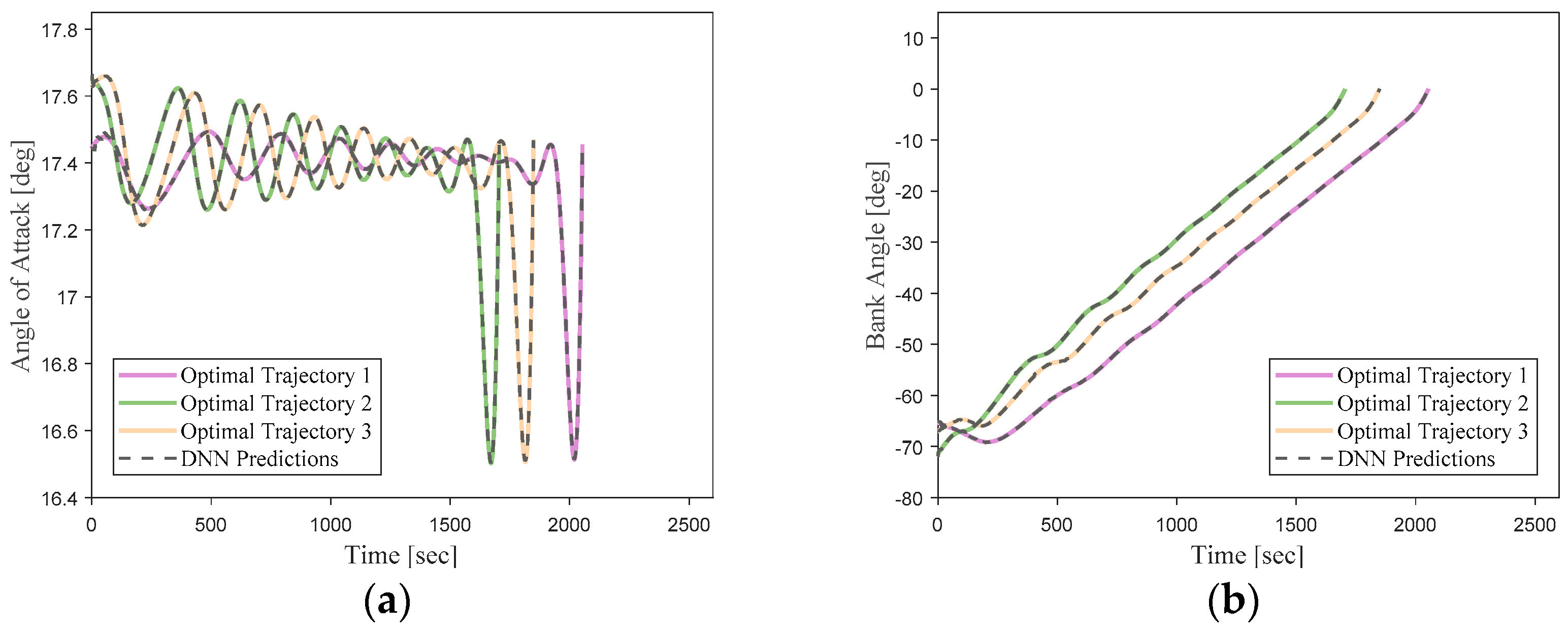
The trained neural network can make predictions based on the current flight state vector x at a given time, providing the control inputs u for the current moment, namely the angle of attack α and bank angle σ . Figure 15 illustrates a comparison between three randomly selected trajectories from the network’s validation dataset and the predicted trajectories generated by the neural network.
The predicted results by the neural network match the optimal trajectories generated using the direct method very closely. This demonstrates a high level of fitting accuracy.
Compared to traditional algorithms, the DNN-based controller offers a simplified computational process and shorter response times. For current DNN models which are developed with TensorFlow in the Python environment, it takes about 0.5 milliseconds to generate a single optimal control instruction on a desktop with an Intel Core i7-12700K processor and a NVIDIA GeForce RTX 3070Ti GPU.
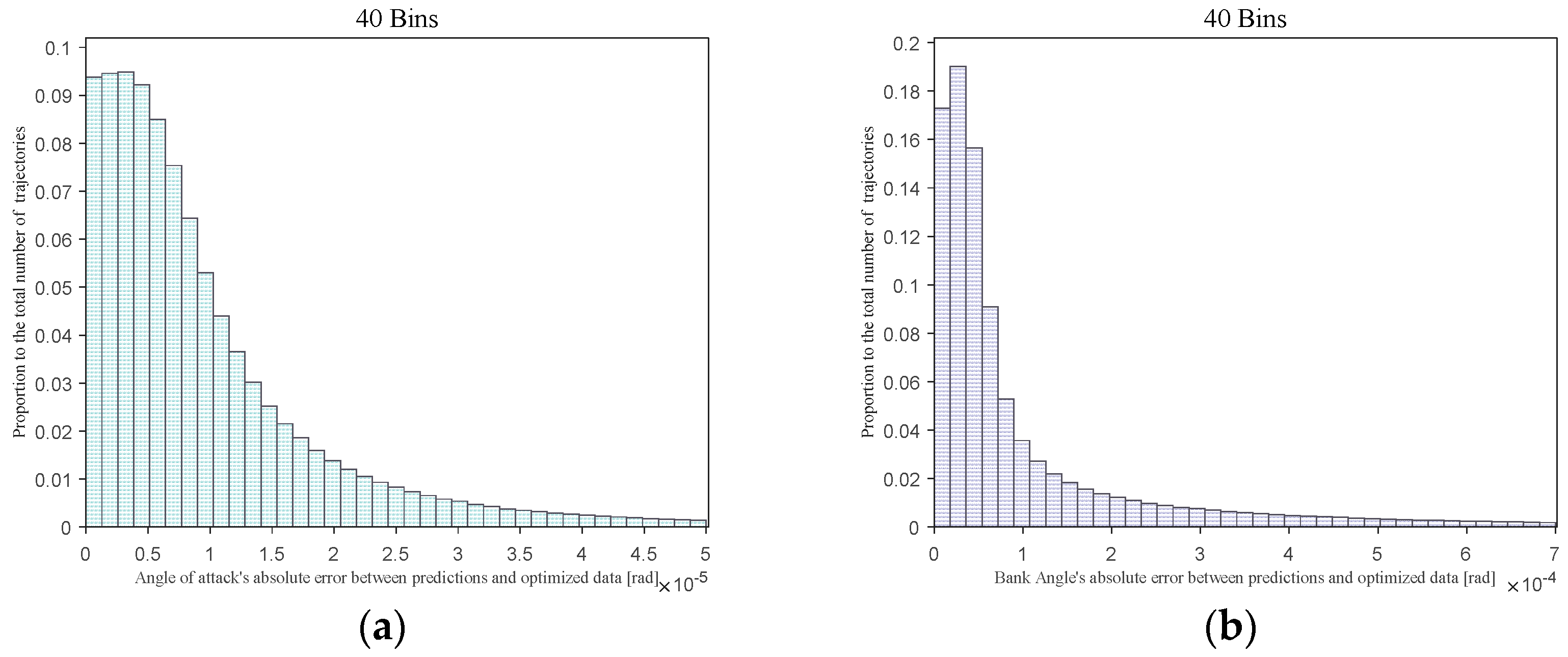
To further quantitatively illustrate the prediction accuracy and errors of the neural network, a histogram of the network prediction absolute errors is presented for another 1000 randomly generated trajectories within the same range as the sample database, as shown in Figure 16.
Figure 16 illustrates the absolute prediction errors of the neural network for optimal actions across 40 bins. The analysis reveals that in the case of angle of attack α , 96.7% of the absolute errors fall below 0.003°, with 58.9% of the errors being less than 0.0005°, and 12.8% not exceeding 0.0001°. The average prediction error is recorded at 0.001°, with a median of 0.0004° and a standard deviation of 0.005°. As for the bank angle σ , 91.2% of the absolute errors are within 0.03°, while 50.9% are limited to 0.003° or less, and 16.8% are below 0.001°. The mean, median, and standard deviation of the prediction errors amount to 0.016°, 0.003°, and 0.11° respectively. The designed DNN model exhibits high accuracy in predicting optimal actions, indicating its potential for achieving precise real-time guidance.

4.2. Analysis of Trajectory Simulation

The preceding section analyzed the direct prediction capability of the network model for optimal actions under the current input state. However, when considering the entire flight trajectory, small prediction errors at each moment can accumulate over the whole flight and may lead to significant deviations between the trajectory predicted based on the network and the optimal trajectory, resulting in suboptimal or failed flight missions. Therefore, it is necessary to conduct trajectory simulations based on neural network predictions to evaluate the network’s performance in a given task scenario. Algorithm 1 provides the pseudo-code for the simulation verification process.
Algorithm 1 Simulation of Trajectory Driving Guided by Deep Neural Networks
1: Load DNN model N e t
2: Set integral step size S
3: Initialize state vector x ( t i ) = x ( t 0 )
4: While r ( t i ) > r ( t f ) :
5:   Preprocess state vector, x ( t i ) p r e p r o c e s s e d
6:   Get predicted control values α p r e d i c t i o n , σ p r e d i c t i o n from N e t
7:   Inverse x ( t i ) p r e p r o c e s s e d to x ( t i )
8:   Put α p r e d i c t i o n , σ p r e d i c t i o n and x ( t i ) into the dynamical equation, obtain x ˙ ( t i )
9:   Integrate for next state vector x ( t i + 1 ) (the RK4 method)
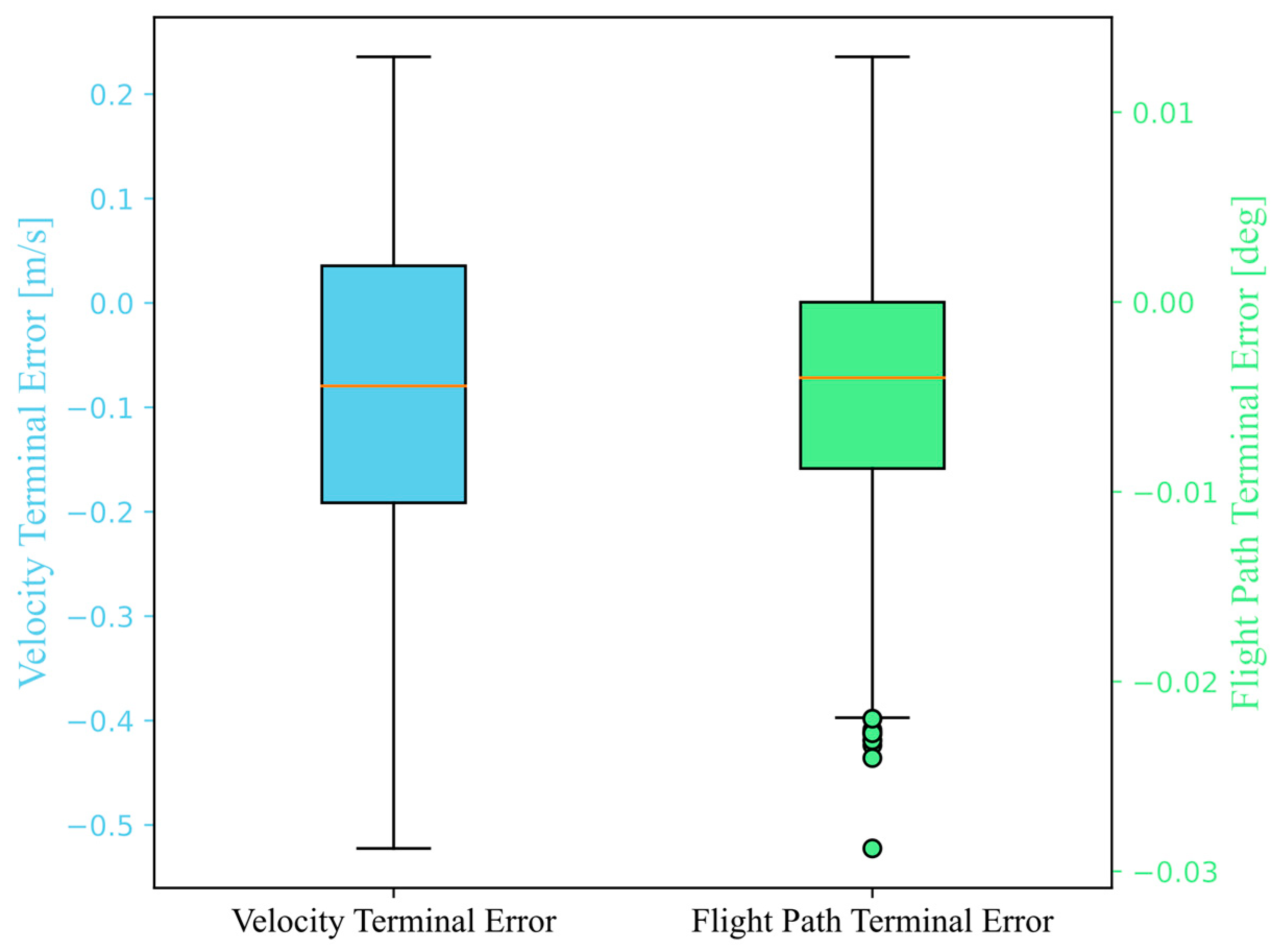
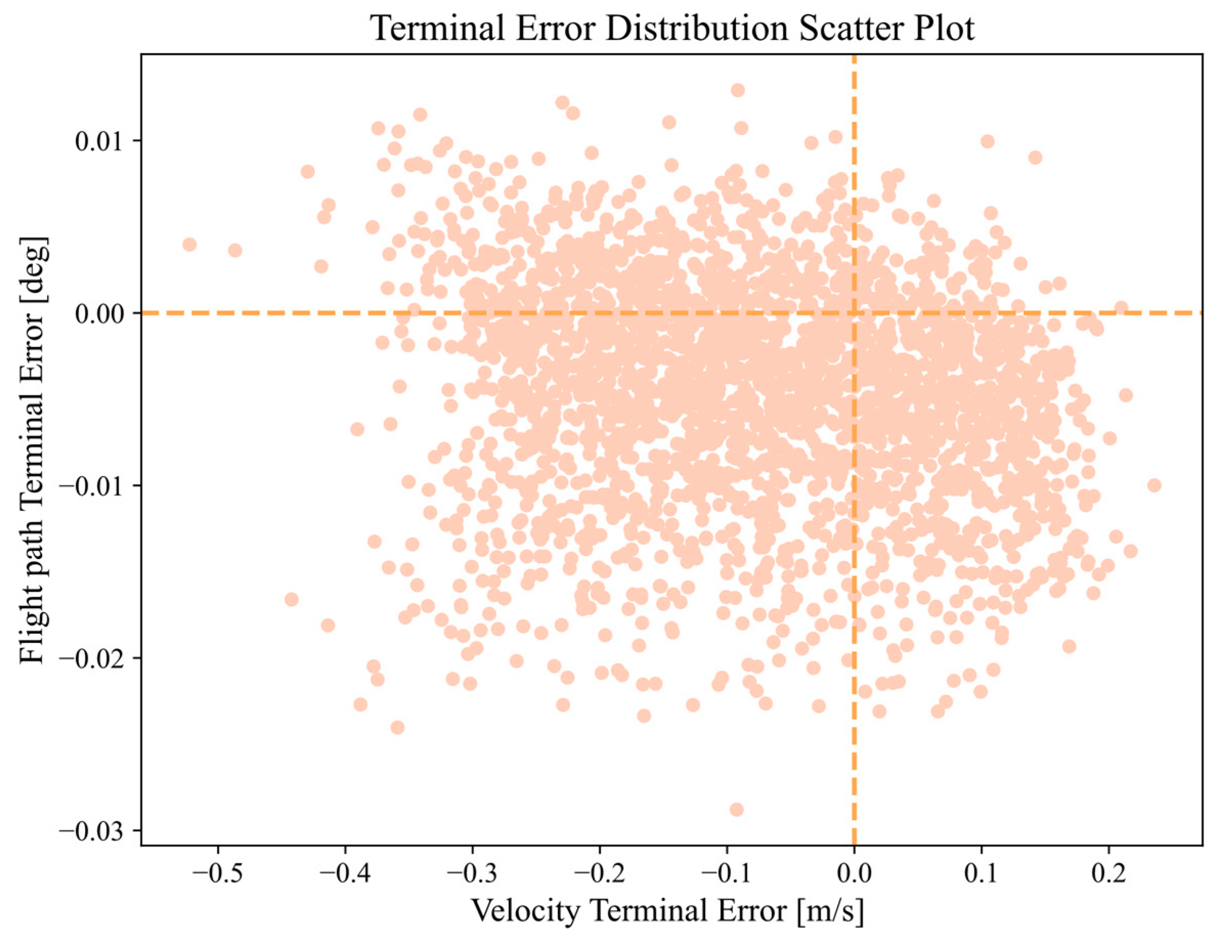
The algorithm implements trajectory generation based on DNNs. By comparing the average absolute errors between the simulated results from the network and the optimal trajectories generated using the direct method, the optimality of the simulated network trajectories can be verified. In order to illustrate the performance of the network, a quantitative analysis of the simulation error of the neural network is conducted. Firstly, the errors in the terminal velocity v ( t f ) and terminal flight path angle γ ( t f ) with terminal constraints in the state vector are calculated. Figure 17 displays the precision analysis of these two variables for trajectories with random initial states. It is worth noting that since the termination condition in Algorithm 1 is the terminal altitude r ( t f ) , there is no precision analysis for the terminal altitude here. Figure 18 depicts the distribution of trajectory terminal errors in simulation.
The maximum, median, and standard deviation of terminal state errors are provided in Table 4.
The terminal velocity error ranges from −0.522 to 0.235 m/s, and the terminal flight path angle error ranges from −0.028° to 0.012°. The maximum terminal velocity error is approximately 0.068% of the terminal velocity, and the maximum terminal bank angle error is approximately 0.57% of the terminal bank angle. Additionally, building upon the analysis of terminal errors in DNN simulation, we also analyzed the MAE of state and control variables based on DNN simulation for these trajectories. The specific data are provided in Table 5.
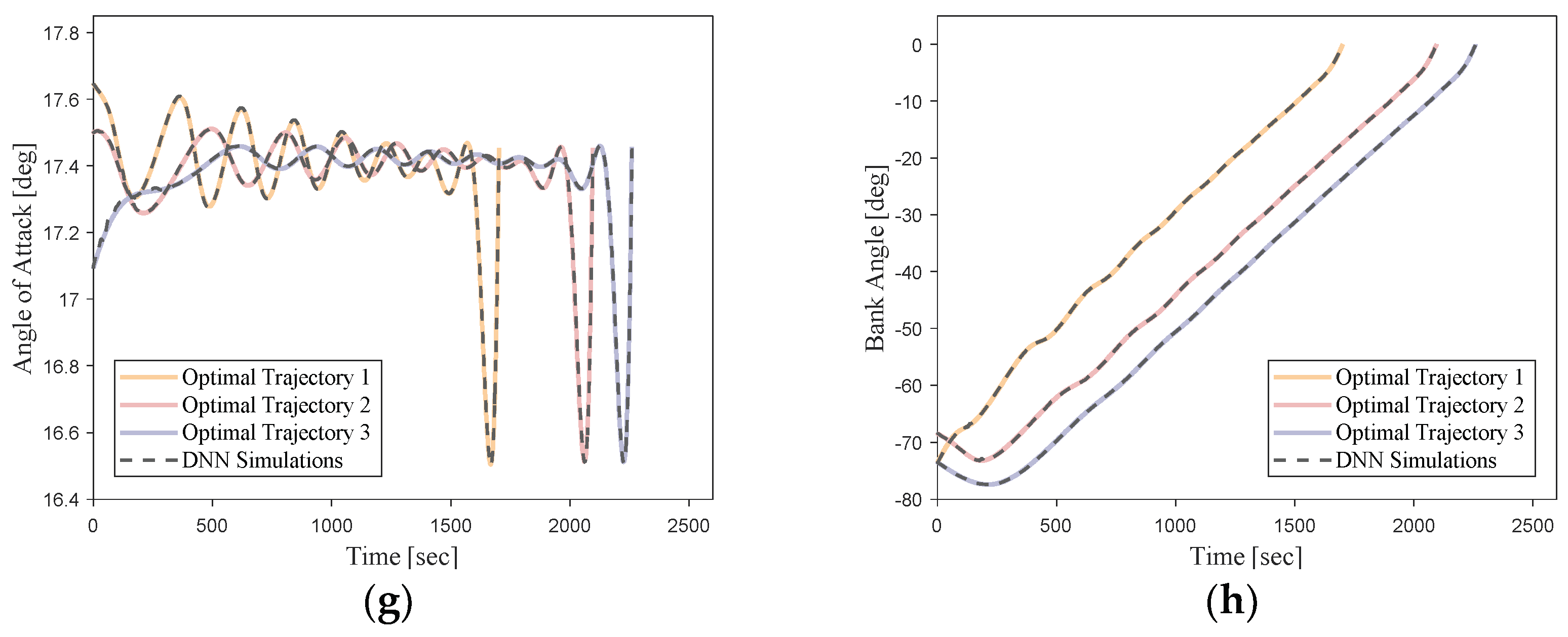
From these error analysis data, it can be shown that the DNN-based optimal trajectory controller for this hypersonic vehicle can ensure trajectory optimality while exhibiting remarkable guidance accuracy under conditions of uncertain initial states. To provide a more intuitive representation of the network’s performance, simulation curves for three trajectories with randomly initialized state vectors are shown in Figure 19.
It can be seen that the simulation trajectories driven by the DNN match the optimal trajectories very well. Under random initial conditions, the DNN can guide the vehicle to complete the flight task along the optimal trajectory for the current state. Additionally, the trajectory simulation time step size of the DNN (0.1 s) is much smaller than the time step size of the optimal trajectories generated using the pseudo-spectral method (about 1 s). This implies that most of the flight state data are not included in the training samples. This indicates that the designed DNN model in this study can effectively learn the nonlinear mapping relationship between the flight state vectors and optimal actions of the hypersonic vehicle in the given task scenario.

4.3. Analysis of Network Robustness

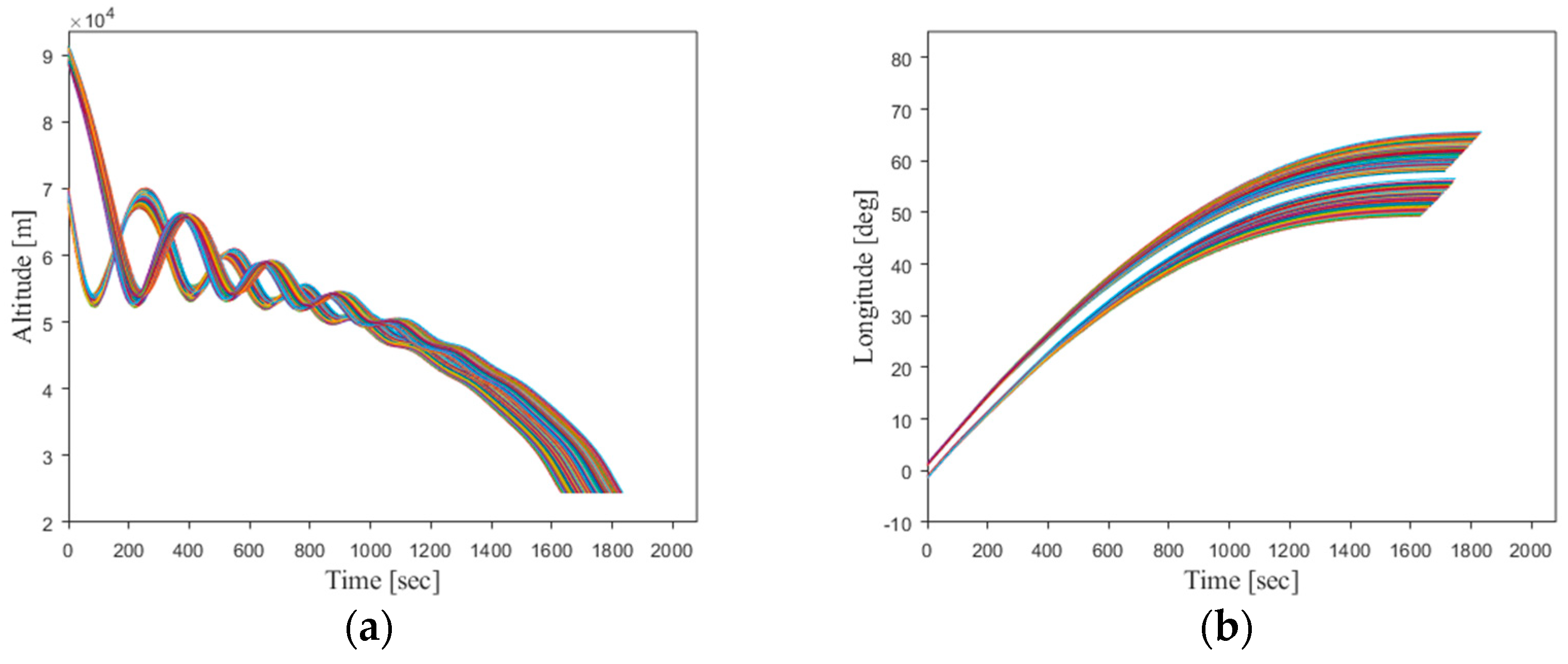
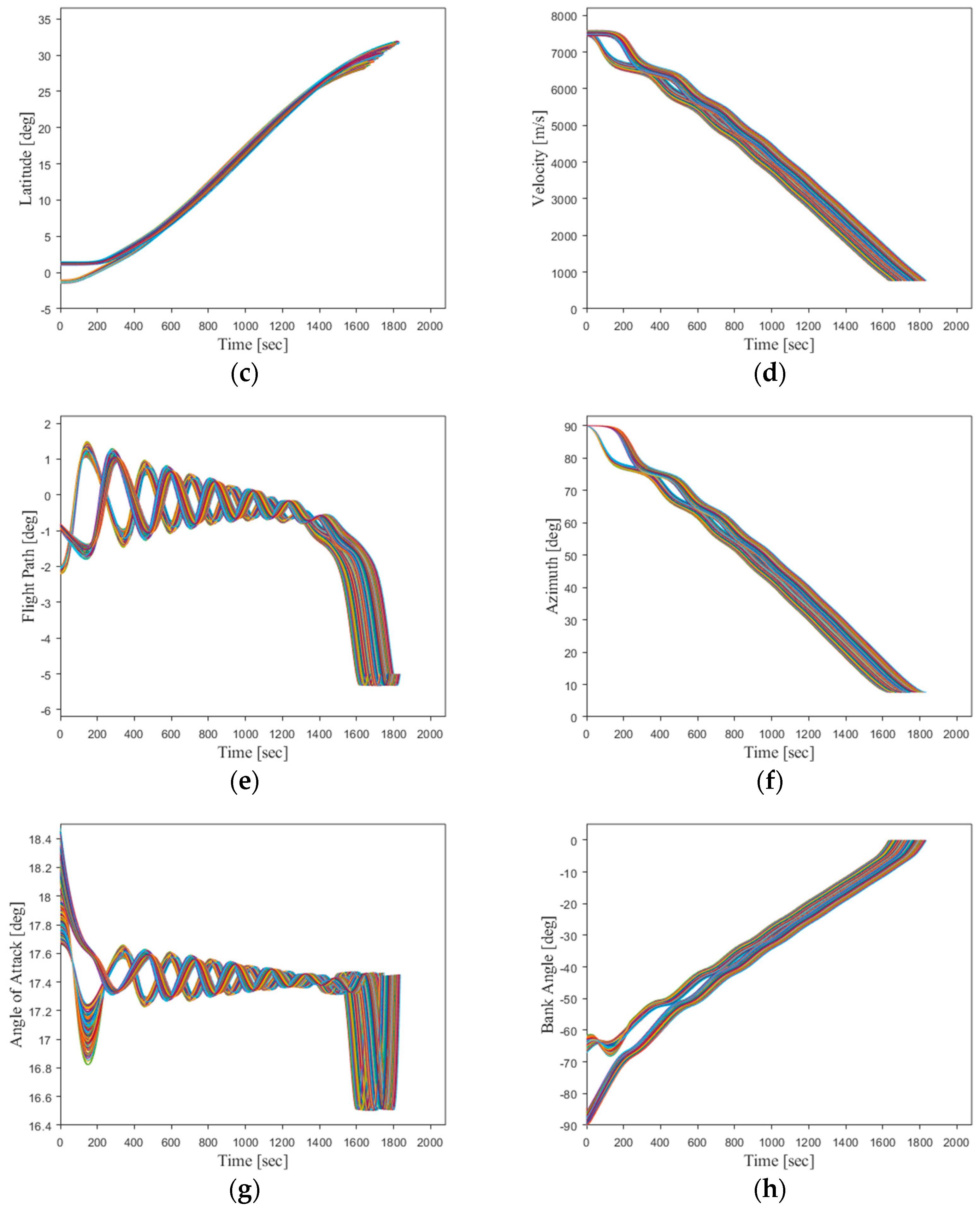
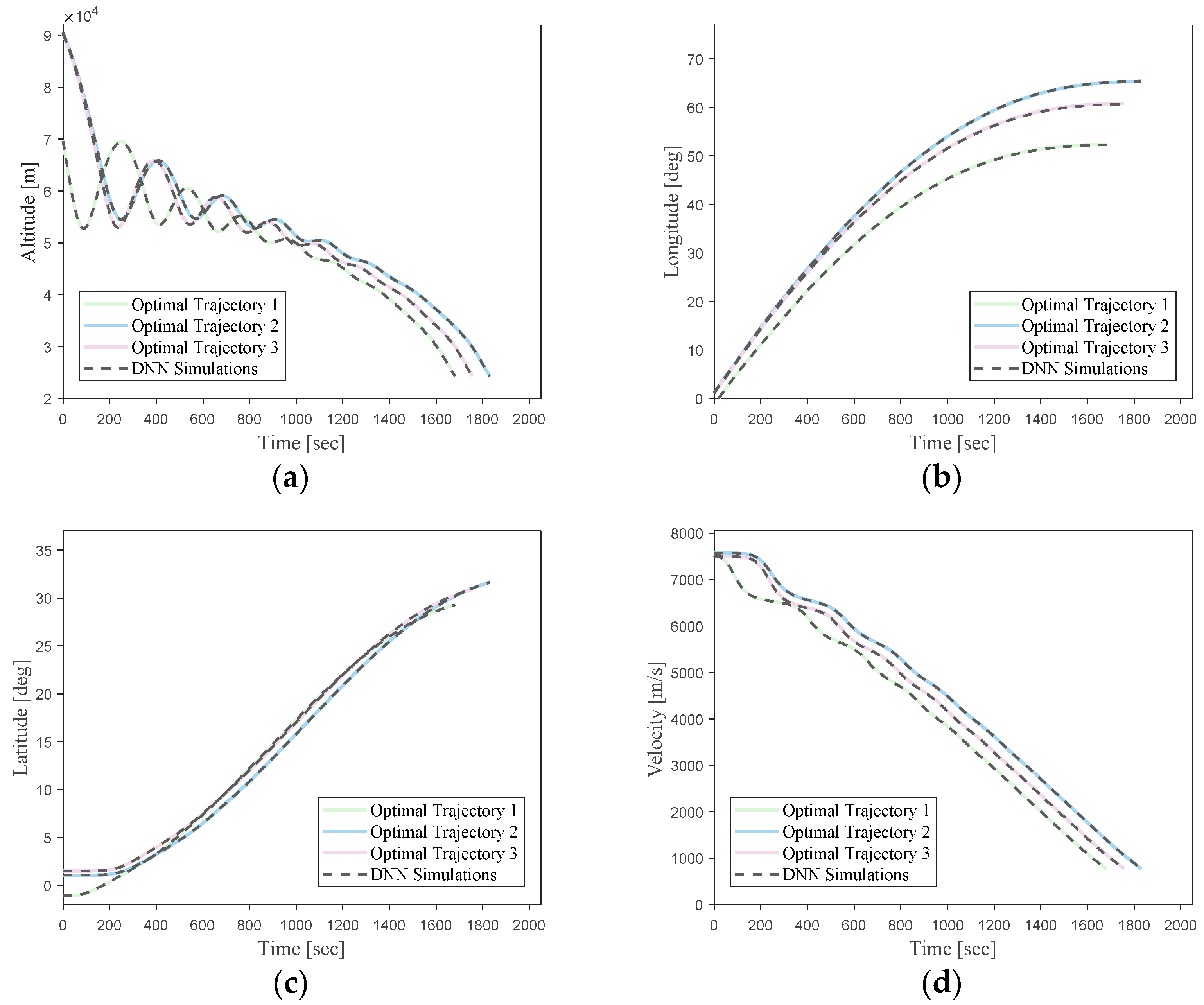
To further explore the network’s performance under unknown initial flight conditions, 500 trajectories are randomly generated outside the original training sample’s initial state range. This is conducted to analyze the network’s generalization capability and its robustness under the uncertainties of the initial flight state. The results are presented in Figure 20.
The new generated trajectories, in comparison to the original training sample data, have significantly extended the range of flight state values at the entry initial point. The specific value ranges for each initial state variable are provided in Table 6.
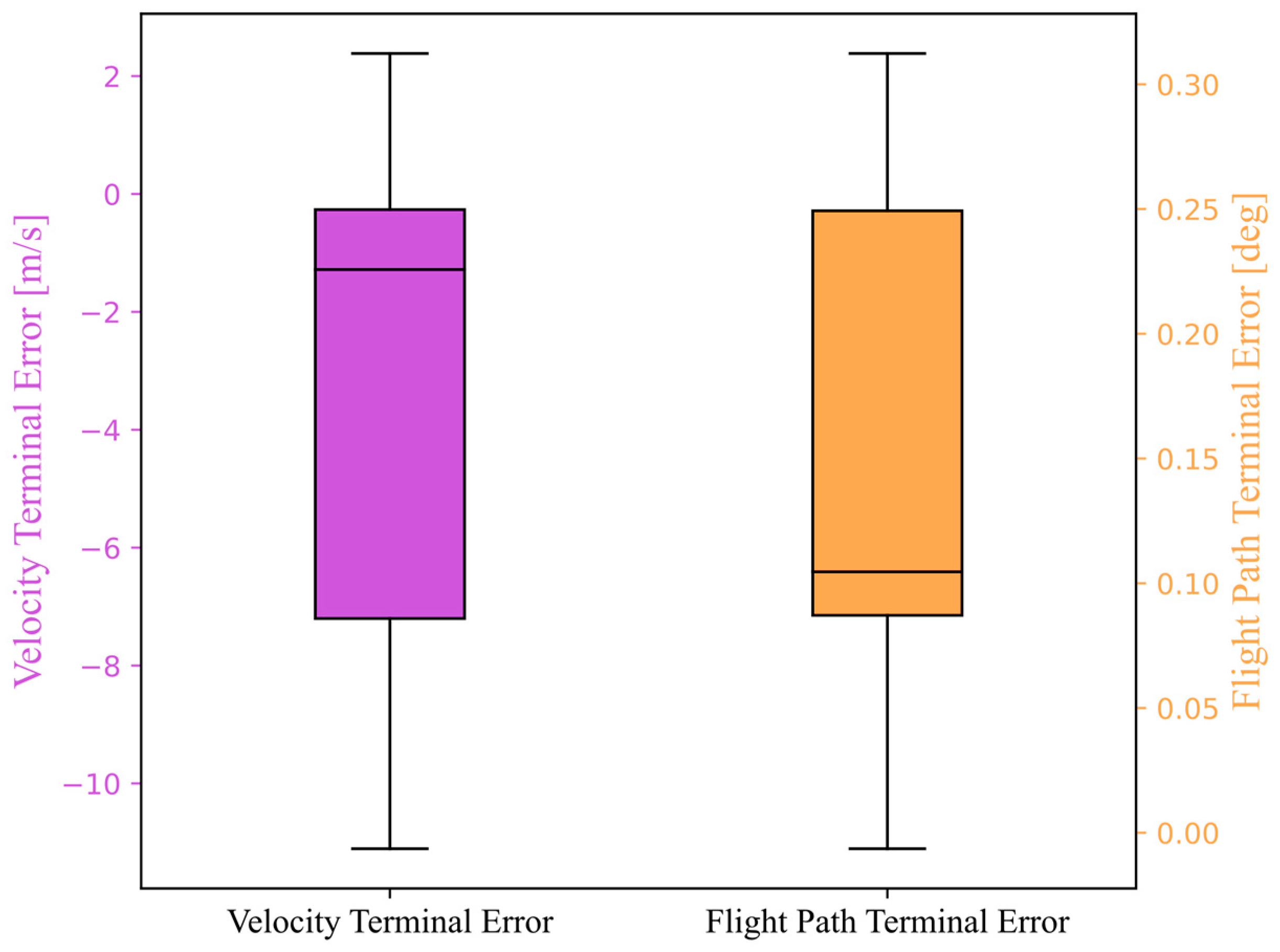
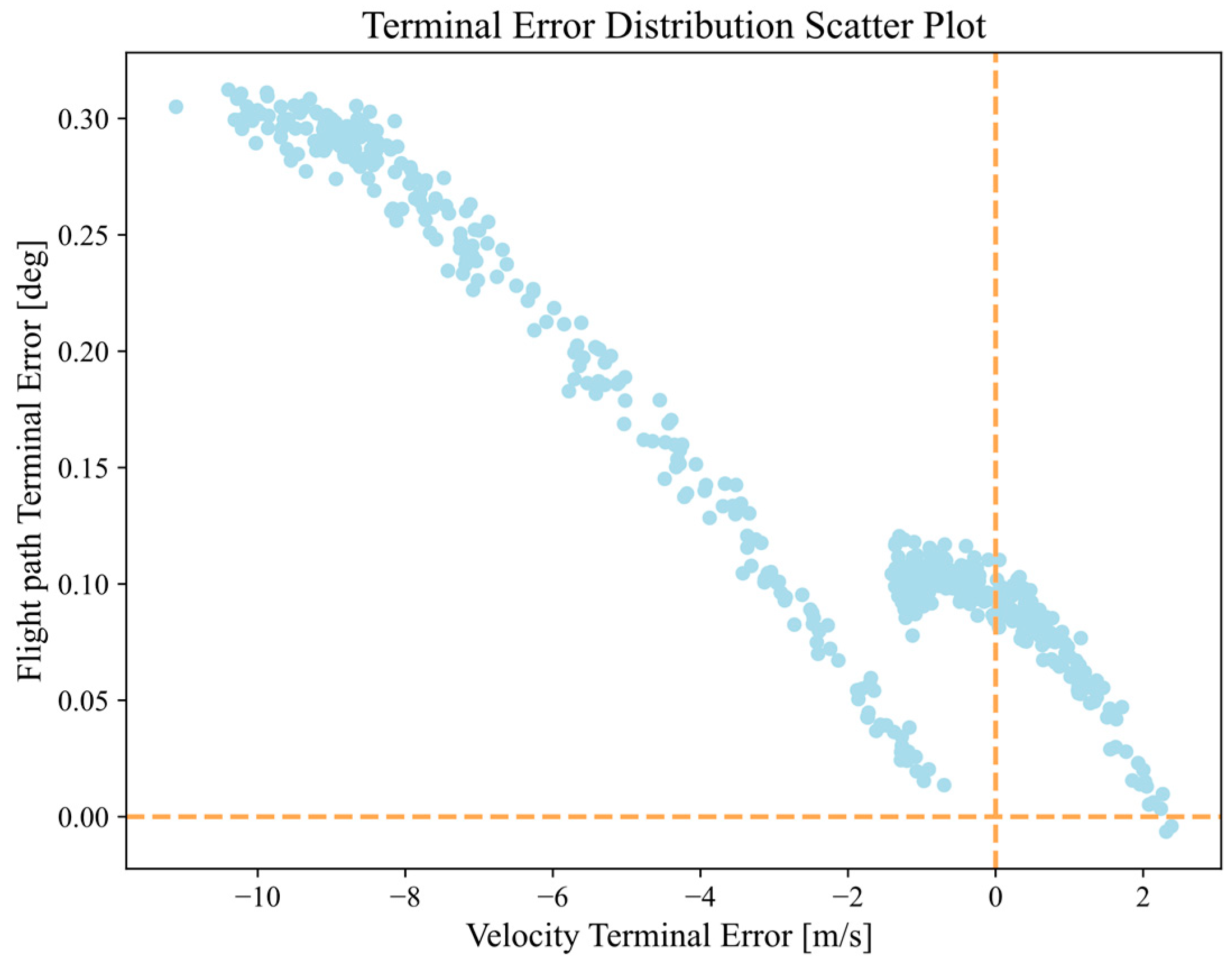
To further illustrate the performance of the DNN-based controller in an unknown initial state region, we conducted a simulation analysis using the DNN model on 500 trajectories from the test dataset. Figure 21 shows the analysis of terminal errors for trajectories generated by the network in the expanded initial state range. It can be observed that although the terminal errors are relatively larger compared to the results in Section 4.2, they remain within an acceptable range. The terminal velocity error ranges within [−11.1076, 2.3835] m/s, and the terminal bank angle error falls within the range of [−0.064, 0.3123] degrees. The maximum, mean, median, and standard deviation of terminal errors are provided in Table 7. Figure 22 depicts the distribution of trajectory simulation terminal errors in the expanded range. It can be observed that the terminal errors of trajectories generated by the DNN within the current expanded range are not normally distributed, and they exhibit a strip-like distribution. It presents two near linear relationships between velocity terminal error and flight path angle terminal error. Table 8 presents a statistical analysis of the MAE for all trajectories generated by the DNN within this expanded state range.
From the error analysis data, it can be observed that even beyond the range of training data, the DNN-based controller is still capable of achieving a certain level of guidance accuracy.
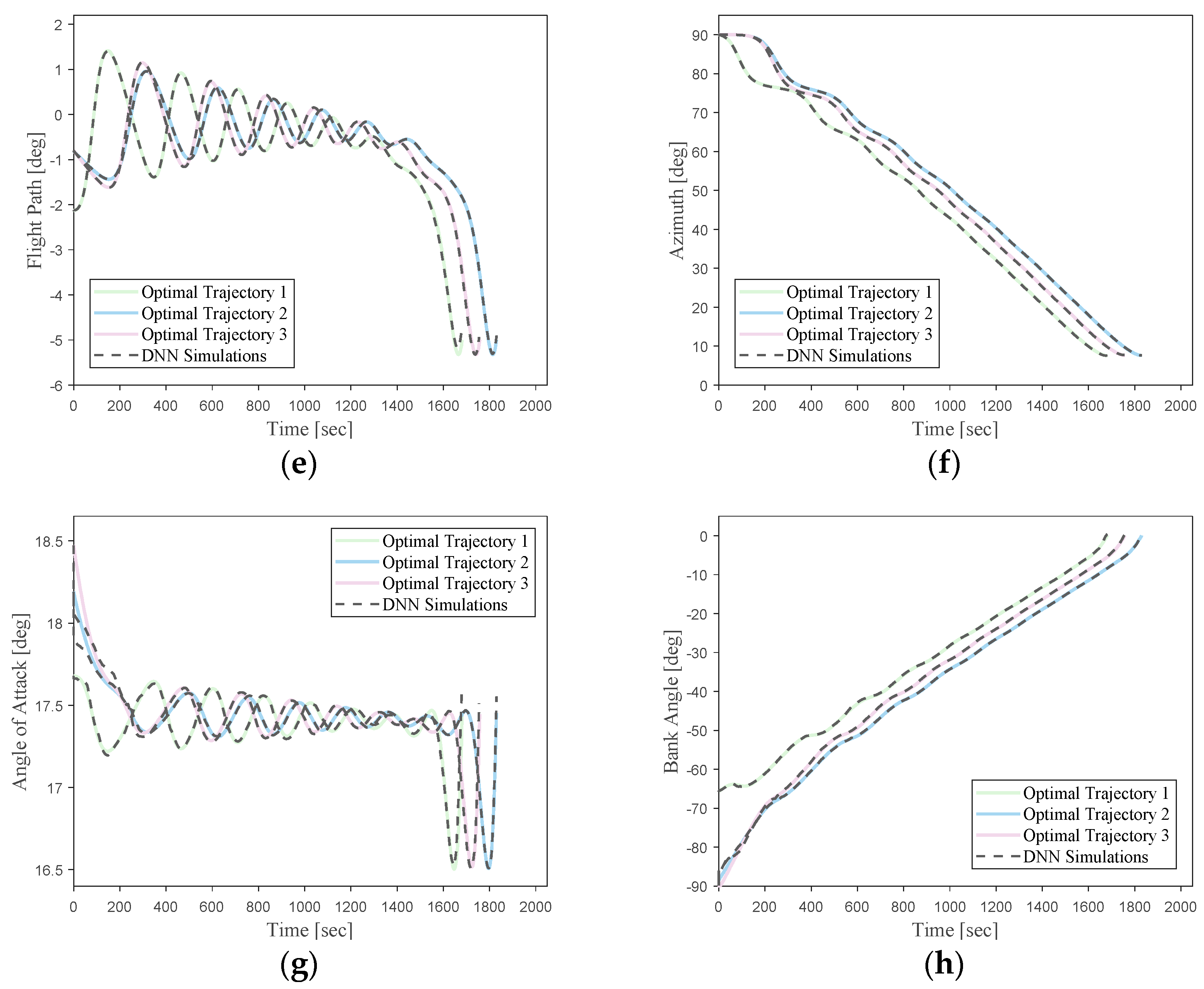
To provide a more visual evaluation of the network’s performance outside the training space, three trajectories were randomly selected within the expanded initial space for online simulations based on the DNN. As shown in Figure 23, a comparison was made between the flight profiles of these trajectories and their corresponding optimal trajectories.
It can be shown that the flight state curves driven by the DNN are smooth and the errors are relatively small. The control variables exhibit larger errors in the initial stages but progressively approach optimal values, with a near-optimal behavior achieved around 270 s. Thus, the proposed DNN-based optimal trajectory controller in this study demonstrates the capability to provide approximate control actions and correct trajectories towards the desired goals, even in cases of significant initial state deviations.
The above results indicate that the designed DNN-based controller can maintain an acceptable level of guidance accuracy even when there are deviations in the initial flight state. It is capable of generating high-quality control commands, demonstrating a certain level of generalization ability and robustness.
5. Conclusions

This paper introduces a method for fast generation of three-dimensional optimal trajectories for hypersonic vehicles using DNNs. It achieves the rapid completion of optimal trajectory planning while maintaining guidance accuracy. This method holds the potential to address the long-standing challenge of balancing the trade-off between fast solution times and optimality in nonlinear optimal control problems. The paper demonstrates how to design and train DNN models to learn the underlying nonlinear mapping relationship between flight states and optimal actions. It verified the authenticity of the sample data and explored the impact of network structure and parameters on the problem. This study encompasses the implementation of a series of simulation experiments aimed at conducting an exhaustive assessment of the trajectory generation capability, generalization proficiency, and robustness of the proposed model. To commence, the optimal trajectory sample data are acquired through the Gauss pseudo-spectral method, and their accuracy is subsequently validated. Subsequently, the cross-validation method is used to iteratively update the network structure and hyperparameters. Optimizers and callback functions are employed to optimize the network model and ensure its optimality. Experimental results demonstrate that the trained network model can rapidly generate guidance commands for optimal flight control with high precision using flight states feedback. Additionally, the model exhibits remarkable generalization ability and robustness, even when the flight states deviate significantly from their initial values at the beginning of the flight.

Author Contributions

Conceptualization, H.L. and C.T.; methodology, H.C.; software, H.L.; validation, H.L., H.C. and Z.J.; formal analysis, X.X.; investigation, H.C.; resources, X.X.; data curation, Z.J.; writing—original draft preparation, H.L. and C.T.; writing—review and editing, H.C., Z.J. and X.X.; visualization, C.T.; supervision, H.C.; project administration, Z.J.; funding acquisition, X.X. All authors have read and agreed to the published version of the manuscript.

Funding

This research was funded by National Defense Basic Scientific Research Program of China, Grant No. 2021103084-M.

Data Availability Statement

All data used during the study appear in the submitted article.

Conflicts of Interest

The authors declare no conflict of interest. The funders had no role in the design of the study; in the collection, analyses, or interpretation of data; in the writing of the manuscript; or in the decision to publish the results.

References

  1. Hinton, G.E.; Osindero, S.; Teh, Y.W. A Fast Learning Algorithm for Deep Belief Nets. Neural Comput. 2006, 18, 1527–1554. [Google Scholar] [CrossRef]
  2. Ackley, D.H.; Hinton, G.E.; Sejnowski, T.J. A Learning Algorithm for Boltzmann Machines. Cogn. Sci. 1985, 9, 147–169. [Google Scholar] [CrossRef]
  3. Krizhevsky, A.; Sutskever, I.; Hinton, G. ImageNet Classification with Deep Convolutional Neural Networks. Commun. ACM 2017, 60, 84–90. [Google Scholar] [CrossRef]
  4. Izzo, D.; Martens, M.; Pan, B. A Survey on Artificial Intelligence Trends in Spacecraft Guidance Dynamics and Control. Astrodynamics 2019, 3, 287–299. [Google Scholar] [CrossRef]
  5. Sanchez-Sanchez, C.; Izzo, D.; Hennes, D. Learning the Optimal State-Feedback Using Deep Networks. In Proceedings of the IEEE Symposium Series on Computational Intelligence (SSCI), Athens, Greece, 6–9 December 2016. [Google Scholar] [CrossRef]
  6. Sanchez-Sanchez, C.; Izzo, D. Real-Time Optimal Control via Deep Neural Networks: Study on Landing Problems. J. Guid. Control Dyn. 2018, 41, 1122–1135. [Google Scholar] [CrossRef]
  7. Izzo, D.; Sprague, C.; Tailor, D. Machine Learning and Evolutionary Techniques in Interplanetary Trajectory Design. arXiv 2018. [Google Scholar] [CrossRef]
  8. Izzo, D.; Tailor, D.; Vasileiou, T. On the Stability Analysis of Deep Neural Network Representations of an Optimal State Feedback. IEEE Trans. Aerosp. Electron. Syst. 2021, 57, 145–154. [Google Scholar] [CrossRef]
  9. Furfaro, R.; Bloise, I.; Orlandelli, M.; Di Lizia, P.; Topputo, F.; Linares, R. A recurrent deep architecture for quasi-optimal feedback guidance in planetary landing. In Proceedings of the First IAA/AAS SciTech Forum on Space Flight Mechanics and Space Structures and Materials, Moscow, Russia, 13–15 November 2018. [Google Scholar]
  10. Furfaro, R.; Bloise, I.; Orlandelli, M.; Di Lizia, P.; Topputo, F.; Linares, R. Deep learning for autonomous lunar landing. In Proceedings of the AAS/AIAA Astrodynamics Specialist Conference, Snowbird, UT, USA, 19–23 August 2018. [Google Scholar]
  11. Cheng, L.; Wang, Z.; Jiang, F.; Zhou, C. Real-Time Optimal Control for Spacecraft Orbit Transfer via Multiscale Deep Neural Networks. IEEE Trans. Aerosp. Electron. Syst. 2019, 55, 2436–2450. [Google Scholar] [CrossRef]
  12. Yin, S.; Li, J.; Cheng, L. Low-Thrust Spacecraft Trajectory Optimization via a DNN-Based Method. Adv. Space Res. 2020, 66, 1635–1646. [Google Scholar] [CrossRef]
  13. Cheng, L.; Wang, Z.; Jiang, F.; Li, J. Fast Generation of Optimal Asteroid Landing Trajectories Using Deep Neural Networks. IEEE Trans. Aerosp. Electron. Syst. 2019, 56, 2642–2655. [Google Scholar] [CrossRef]
  14. Cheng, L.; Wang, Z.; Song, Y.; Jiang, F. Real-Time Optimal Control for Irregular Asteroid Landings Using Deep Neural Networks. Acta Astronaut. 2020, 170, 66–79. [Google Scholar] [CrossRef]
  15. You, S.; Wan, C.; Dai, R.; Rea, J. Learning-Based Onboard Guidance for Fuel-Optimal Powered Descent. J. Guid. Control Dyn. 2021, 44, 601–613. [Google Scholar] [CrossRef]
  16. Wang, Z.; Michael, J.G. Constrained trajectory optimization for planetary entry via sequential convex programming. J. Guid. Control Dyn. 2017, 40, 2603–2615. [Google Scholar] [CrossRef]
  17. Wang, Z.; Ye, L. Improved sequential convex programming algorithms for entry trajectory optimization. J. Spacecr. Rocket. 2020, 57, 1373–1386. [Google Scholar] [CrossRef]
  18. Shi, Y.; Wang, Z. Onboard Generation of Optimal Trajectories for Hypersonic Vehicles Using Deep Learning. J. Spacecr. Rocket. 2021, 58, 400–414. [Google Scholar] [CrossRef]
  19. Wang, J.; Wu, Y.; Liu, M.; Yang, M.; Liang, H. A Real-Time Trajectory Optimization Method for Hypersonic Vehicles Based on a Deep Neural Network. Aerospace 2022, 9, 188. [Google Scholar] [CrossRef]
  20. Gao, J.; Shi, X.; Cheng, Z.; Xiong, J.; Liu, L.; Wang, Y.; Yang, Y. Reentry trajectory optimization based on Deep Reinforcement Learning. In Proceedings of the 2019 Chinese Control and Decision Conference (CCDC), Nanchang, China, 3–5 June 2019. [Google Scholar]
  21. Wu, T.; Wang, H.; Liu, Y.; Ren, B.; Yu, Y. A Reentry Guidance Algorithm Based on Deep Reinforcement Learning and Altitude Rate Feedback. Unmanned Syst. Technol. 2022, 5, 1–13. [Google Scholar] [CrossRef]
  22. Solari, M. Reinforcement Learning Guidance for Pinpoint Landing on Mars. Master’s Thesis, Delft University of Technology, Delft, The Netherlands, 26 July 2017. [Google Scholar]
  23. Wang, R.; Hui, J.; Yu, Q.; Li, T. Research of LSTM Model-Based Intelligent Guidance of Flight Aircraft. Chin. J. Theor. Appl. Mech. 2021, 53, 2047–2057. [Google Scholar] [CrossRef]
  24. Cheng, L.; Jiang, F.; Wang, Z.; Li, J. Multiconstrained Real-Time Entry Guidance Using Deep Neural Networks. IEEE Trans. Aerosp. Electron. Syst. 2021, 57, 325–340. [Google Scholar] [CrossRef]
  25. Patterson, M.; Rao, A. GPOPS-II: A MATLAB Software for Solving Multiple-Phase Optimal Control Problems Using Hp-Adaptive Gaussian Quadrature Collocation Methods and Sparse Nonlinear Programming. ACM Trans. Math. Softw. 2014, 41, 1–37. [Google Scholar] [CrossRef]
  26. Betts, J. Practical Methods for Optimal Control and Estimation Using Nonlinear Programming; Society for Industrial and Applied Mathematics Press: Philadelphia, PA, USA, 2009; pp. 147–152. [Google Scholar]
  27. Nair, V.; Hinton, G.E. Rectified Linear Units Improve Restricted Boltzmann Machines. In Proceedings of the 27th International Conference on International Conference on Machine Learning, Madison, WI, USA, 21–24 June 2010. [Google Scholar]
  28. Kingma, D.; Ba, J. Adam: A Method for Stochastic Optimization. arXiv 2014. [Google Scholar] [CrossRef]
  29. He, T.; Zhang, Z.; Zhang, H.; Zhang, Z.; Xie, J.; Li, M. Bag of Tricks for Image Classification with Convolutional Neural Networks. In Proceedings of the 2019 IEEE/CVF Conference on Computer Vision and Pattern Recognition (CVPR), Long Beach, CA, USA, 15–20 June 2019. [Google Scholar] [CrossRef]
  30. Darken, C.; Chang, J.; Moody, J. Learning Rate Schedules for Faster Stochastic Gradient Search. In Neural Networks for Signal Processing II, Proceedings of the 1992 IEEE Workshop, Helsingoer, Denmark, 31 August–2 September 1992; IEEE Press: Piscataway, NJ, USA, 1992. [Google Scholar] [CrossRef]
Figure 1. Max cross-range entry flight.
Aerospace 10 00931 g001
Figure 2. Profiles of the states. (a) Altitude–time curve; (b) Longitude–time curve; (c) Latitude–time curve; (d) Velocity–time curve; (e) Flight path–time curve; (f) Azimuth–time curve.
Aerospace 10 00931 g002aAerospace 10 00931 g002b
Figure 3. Profiles of the optimal control. (a) Angle of attack–time curve; (b) Bank angle–time curve.
Aerospace 10 00931 g003
Figure 4. State of training and test data. (a) Altitude–time curve; (b) Longitude−time curve; (c) Latitude–time curve; (d) Velocity–time curve; (e) Flight path–time curve; (f) Azimuth–time curve.
Aerospace 10 00931 g004aAerospace 10 00931 g004b
Figure 5. Optimal control of training and test data. (a) Angle of attack–time curve; (b) Bank angle–time curve.
Aerospace 10 00931 g005
Figure 6. The flowchart of the trajectory simulation process.
Aerospace 10 00931 g006
Figure 7. Trajectory comparison between simulated and numerically optimal. (a) Altitude–time curve; (b) Longitude–time curve; (c) Latitude–time curve; (d) Velocity–time curve; (e) Flight path–time curve; (f) Azimuth–time curve.
Aerospace 10 00931 g007aAerospace 10 00931 g007b
Figure 8. DNN-based trajectory optimization method.
Aerospace 10 00931 g008
Figure 9. DNN online application diagram scheme.
Aerospace 10 00931 g009
Figure 10. Training histories of neural network with different network architectures. (a) Training loss; (b) Validation loss.
Aerospace 10 00931 g010
Figure 11. Training histories of neural network with different minibatch sizes. (a) Training loss; (b) Validation loss.
Aerospace 10 00931 g011
Figure 12. Training histories of neural network with different initial learning rates. (a) Training loss; (b) Validation loss.
Aerospace 10 00931 g012
Figure 13. Comparison diagram of introducing callback function. (a) Training loss; (b) Validation loss.
Aerospace 10 00931 g013
Figure 14. Training histories of neural network with different patience levels. (a) Training loss; (b) Validation loss.
Aerospace 10 00931 g014
Figure 15. Comparison between optimized and DNN-predicted values of the control variable. (a) Angle of attack–time curve; (b) Bank angle–time curve.
Aerospace 10 00931 g015
Figure 16. Absolute error histograms of the DNN prediction of optimal action. (a) The absolute error of the angle of attack; (b) The absolute error of the bank angle.
Aerospace 10 00931 g016
Figure 17. Terminal error analysis of trajectory simulation.
Aerospace 10 00931 g017
Figure 18. Terminal error distribution scatter plot.
Aerospace 10 00931 g018
Figure 19. Comparison between DNN-driven Trajectory and Optimal Trajectory. (a) Altitude–time curve; (b) Longitude–time curve; (c) Latitude–time curve; (d) Velocity–time curve; (e) Flight path–time curve; (f) Azimuth–time curve; (g) Angle of attack–time curve; (h) Bank angle–time curve.
Aerospace 10 00931 g019aAerospace 10 00931 g019b
Figure 20. Optimal trajectory in expanded random range. (a) Altitude–time curve; (b) Longitude–time curve; (c) Latitude–time curve; (d) Velocity–time curve; (e) Flight path–time curve; (f) Azimuth–time curve; (g) Angle of attack–time curve; (h) Bank angle–time curve.
Aerospace 10 00931 g020aAerospace 10 00931 g020b
Figure 21. Terminal error analysis of trajectory simulation in expanded range.
Aerospace 10 00931 g021
Figure 22. Terminal error distribution scatter plot in expanded range.
Aerospace 10 00931 g022
Figure 23. DNN-driven trajectory in expanded random range. (a) Altitude–time curve; (b) Longitude–time curve; (c) Latitude–time curve; (d) Velocity–time curve; (e) Flight path–time curve; (f) Azimuth–time curve; (g) Angle of attack–time curve; (h) Bank angle–time curve.
Aerospace 10 00931 g023aAerospace 10 00931 g023b
Table 1. Boundary conditions for nominal flight conditions.
Initial ParameterValueTerminal ParameterValue
Geocentric distance r ( t 0 ) 6,450,451.92 mGeocentric distance r ( t f ) 6,395,587.92 m
Longitude θ ( t 0 ) Longitude θ ( t f ) Free
Latitude ϕ ( t 0 ) Latitude ϕ ( t f ) Free
Velocity v ( t 0 ) 7803 m/sVelocity v ( t f ) 762 m/s
Flight path angle γ ( t 0 ) −1°Flight path angle γ ( t f ) −5°
Heading angle ψ ( t 0 ) 90°Heading angle ψ ( t f ) Free
Table 2. Range of initial state values for trajectories.
ParameterValue Range
Initial geocentric distance r ( t 0 ) 6,441,307.92~6,459,595.92 m
Initial longitude θ ( t 0 ) −1°~1°
Initial latitude ϕ ( t 0 ) −1°~1°
Initial velocity v ( t 0 ) 7589.52~8016.24 m/s
Initial flight path angle γ ( t 0 ) −2°~−1°
Table 3. Statistics for state variable absolute error analysis.
ParameterMaxMeanMedianStandard
Deviation
Altitude47.6 m7.47 m6.33 m5.71 m
Longitude0.05°0.002°0.0009°0.003°
Latitude0.01°0.0009°0.0005°0.001°
Velocity3.15 m/s0.3 m/s0.22 m/s0.28 m/s
Flight path0.03°0.002°0.002°0.002°
Azimuth0.13°0.006°0.004°0.008°
Table 4. Statistics for terminal guidance error analysis.
ParameterMaxMeanMedianStandard
Deviation
Terminal velocity
error
−0.522 m/s−0.078 m/s−0.079 m/s0.138 m/s
Terminal flight path error−0.028°−0.004°−0.003°0.006°
Table 5. Statistics for state and control variable MAE analysis.
ParameterMaxMeanMedianStandard
Deviation
MAE of altitude756.8 m11.63 m8.4 m28.032 m
MAE of longitude0.522°0.006°0.003°0.017°
MAE of latitude0.254°0.003°0.001°0.008°
MAE of velocity57.1 m/s0.72 m/s0.434 m/s1.964 m/s
MAE of flight path0.122°0.003°0.002°0.005°
MAE of azimuth0.724°0.009°0.006°0.025°
MAE of angle of
attack
0.045°0.001°0.001°0.002°
MAE of bank angle0.854°0.014°0.009°0.031°
Table 6. Out-of-range trajectory initial state value range.
ParameterValue Range
Initial geocentric distance r ( t 0 ) 6,438,259.92~6,441,307.92 m,
6,459,595.92~6,462,643.92 m
Initial longitude θ ( t 0 ) −1.5°~−1°, 1°~1.5°
Initial latitude ϕ ( t 0 ) −1.5°~−1°, 1°~1.5°
Initial flight path angle γ ( t 0 ) −2.2°~−2°, −1°~−0.8°
Table 7. Terminal error analysis data within expanded range.
ParameterMaxMeanMedianStandard
Deviation
Terminal velocity
error
−11.107 m/s−3.232 m/s−1.283 m/s3.804 m/s
Terminal flight path error0.312°0.149°0.105°0.091°
Table 8. MAE data of state variables and control variables within expanded range.
ParameterMaxMeanMedianStandard
Deviation
MAE of altitude631.6 m123 m59.2 m138.8 m
MAE of longitude0.242°0.053°0.046°0.042°
MAE of latitude0.107°0.025°0.021°0.019°
MAE of velocity30.3 m/s6.74 m/s5.75 m/s5.34 m/s
MAE of flight path0.129°0.029°0.016°0.028°
MAE of azimuth0.423°0.094°0.077°0.076°
MAE of angle of
attack
0.053°0.019°0.016°0.009°
MAE of bank angle0.576°0.187°0.17°0.094°
Disclaimer/Publisher’s Note: The statements, opinions and data contained in all publications are solely those of the individual author(s) and contributor(s) and not of MDPI and/or the editor(s). MDPI and/or the editor(s) disclaim responsibility for any injury to people or property resulting from any ideas, methods, instructions or products referred to in the content.