Structural Stability Analysis of Underwater High-Speed Moving Vehicles in Supercavity Flow Velocity

Abstract

The purpose of this paper is to analyze the structural stability of an underwater high-speed vehicle. The drag characteristics of a moving body moving at high speed in water were analyzed, and a stability analysis of the structure was performed by applying the non-conservative property according to the driven force in a rocket propulsion environment. To this end, the fluid characteristics that enable high-speed maneuvering in an underwater environment were described, and the structural stability was analyzed by simplifying modeling by increasing the resulting drag. In addition, for high-speed underwater movement, an analysis of the following force according to drag and axial load and the effect on structural stability was conducted by simplifying the structure attached to a specific location when a supercavitation occurs.

1. Introduction

The maximum speed of underwater vehicles with large slenderness, such as submarines and torpedoes, is limited by the significant friction drag on the hull surface. The maximum speed of an underwater vehicle does not exceed 40 m/s, and actual operating systems could not achieve more than half of that speed. The characteristics of underwater vehicles that move at low speeds have advantages in terms of underwater acoustics and hydrodynamics, but underwater weapons of modern torpedoes or submarines require high-speed propulsion. In response to this demand, the former Soviet Union developed a torpedo named Shkval in 1977, and the maximum underwater speed reached up to 100 m/s. Supercavitation occurs in these underwater vehicles due to high speed. Supercavitation is a phenomenon in which fluid pressure air bubbles are created on the surface of a moving body due to water vapor pressure when a certain speed is exceeded in water. These air bubbles can cause noise and a decrease in speed, causing structural instability due to changes in the cavitation area depending on the speed of the moving body [1]. Recently, research on the surface flow of underwater vehicles has continued, and in 1997, the U.S. Navy NUWC (Naval Undersea Warfare Center) succeeded in obtaining a speed of 1549 m/s, which is close to the speed of sound in water [2]. However, increasing thrust to increase speed basically causes the tangential follower force caused by thrust. Due to these load characteristics, structures can become statically or dynamically unstable [3]. In other words, in the case of an elastic body subjected to a force whose magnitude changes over time, structural stability analysis has become important, taking into account not only static stability but also dynamic stability.

Previously, high-speed moving objects in water had only the ability to move straight due to difficulty in attitude control. However, technological advancements and operational performance requirements require that attitude control be possible at high speeds underwater, and control techniques for this are continuously evolving [4,5]. Currently, attitude control techniques include a method of controlling attitude by changing the underwater incidence angle of the cavitator, and a method of controlling attitude by protruding a control pin outside the underwater supercavity is being developed [6,7].

In this study, structural stability analysis was performed by applying a method that allows direct attitude control by protruding a controller outside the supercavity. The structure (or controller) at a specific location outside the supercavity is affected by the bulk modulus of elasticity. In particular, when structural instability occurs depending on the characteristics of the follower force, the lift coefficient value changes according to the change in the fluid incidence angle of the fin. This change in coefficient was assumed to be an intermediate elastic support effect. Using the intermediate elastic support effect and a model in which the entire beam receives elastic support, we attempted to evaluate the stability of the structure through analysis of structural vibration and stability according to the elastic support location. For this purpose, the natural frequencies and modes of the structure were numerically analyzed using the finite-element method. However, the fluid characteristics were simply considered as elastic support, and only the trend of influence on the structure was identified. As an example of the mathematical modeling process of a system receiving such a follower force, Beck considered an ideal cantilever (Beck’s beam) receiving a tangential follower force (P) at the end, as shown in Figure 1 [8]. As shown in the figure, Beck’s beam does not exactly match the actual structure, but it is assumed to be a cantilever beam by further simplifying the free-free beam that receives the following force. In real flexible structures, the mass, stiffness, and axial pressure distribution are variable. On the other hand, if the beam is assumed to be a cantilever and the mass, stiffness, and axial pressure of the structure are expressed as uniform distributions, analysis becomes easier. Basically, it was confirmed that Beck’s beam can be expressed with basic stability and bending flutter corresponding to a free-free beam. In addition, since experiments to verify the dynamic stability of the free-free beam are quite difficult, it was considered a cantilever beam, and it was proven that the theoretical analysis results and the experimental results were consistent [9].

2. Theoretical Analysis

2.1. Mathematical Model

The mathematical model in Figure 2 shows that the underwater supercavity body is concentrated in drag by the cavitator at the bow, which can be simplified into a cantilever (Beck’s beam) with a fixed end [8]. The underwater high-speed vehicle has an external protruding structure, and this structure also acquires fluid characteristics due to a supercavity. At this time, water flowing into the external structure due to re-entrant affects the drag of the aircraft. This is due to the re-inflow of water into the cavity area, resulting in cavitation shedding. Due to cavitation shedding, the structure comes into contact with water instead of steam, causing it to vibrate significantly, as shown in the picture. As the structure (body) comes into contact with water, which has a higher pressure than water vapor, the drag increases; conversely, the more it comes into contact with water vapor, the drag decreases.

In this way, a cantilever beam (Beck’s beam) with a constant cross-section of the entire length subjected to a concentrated driven force was placed on an elastic foundation and was modeled as having a support point at a random position from the fixed end. Here, the bending stiffness of the beam is EI, the mass of the beam per unit length is m, the spring constant of the elastic foundation is k, and the spring constant of the partial elastic foundation is k₁. Also, E* is time and γ is the internal material attenuation coefficient.

2.2. Equation of Motion

In order to obtain the governing equations of motion for the model in Figure 2, the extended Hamilton principle was used as follows.

$$\xi \mathsf{\delta }{\int }_{t_1}^{t_2}\left(T+W_c-U\right)dt+{\int }_{t_1}^{t_2}\left(\delta W_{id}+\delta W_{nc}\right)dt=0$$

(1)

Here, T is the kinetic energy, W_c is the work due to the conservative component of the force acting on the free end, U is the elastic potential energy, $\mathsf{\delta }{W}_{id}$ is the virtual work due to internal damping, and $\mathsf{\delta }{W}_{nc}$ is the virtual work due to the non-conservative component.

$$T={\int }_0^L\frac{m}{2}{\left(\frac{\partial y}{\partial t}\right)}^{2}dx$$

(2)

$$W_c={\int }_0^L\frac{p}{2}{\left(\frac{\partial y}{\partial x}\right)}^{2}dx,$$

(3)

$$U={\int }_0^L\frac{EI}{2}{\left(\frac{{\partial }^{2}y}{\partial x^2}\right)}^{2}dx+{\int }_0^L\frac{k}{2}{y}^{2}dx,$$

(4)

$${\delta W}_{id}=-{\int }_0^L{E}^{*}{\left(\frac{{\partial }^{2}y}{\partial x^2}\right)}^{2}dx+{\int }_0^L\frac{k}{2}{y}^{2}dx,$$

(5)

$${\delta W}_{nc}=-p{\left(\frac{\partial y}{\partial x}\right)}_{x=L}dy$$

(6)

To simplify the calculations, the following non-dimensionalized coordinates and parameters were used here.

$$\xi =\frac{x}{L},\mathrm{\eta }=\frac{y}{L}, \tau =\frac{t}{L^2}\sqrt{\frac{EI}{m}},{\xi }_1=\frac{x_1}{L}, p=\frac{P{L}^2}{EI}, \kappa =\frac{k{L}^4}{EI}, {\kappa }_1=\frac{k{x}_1^4}{EI}, \gamma =\frac{E^{*}}{E{L}^2}\sqrt{\frac{EI}{m_f+m_p}}$$

(7)

Here, $\xi$ and $\mathrm{\eta }$ are the coordinates of $x$ and $y$, respectively; $m$ is the mass per unit length; $E^{*}$ is the internal material damping coefficient; $\tau$ is time; $p$ is the driven force; $\gamma$ is the internal damping; $\kappa$ is a dimensionless parameter representing the overall elastic support spring of the beam; and ${\kappa }_1$ is a dimensionless parameter representing the elastic support spring of the intermediate support point. Although ${\kappa }_1$ is not mentioned in the formula, the calculation program calculates it by considering that the deflection at the position of the support point is 0. Substituting Equations (2) to (6) into Equation (1) and then substituting the dimensionless parameters and coordinates of Equation (7), the following equation is obtained.

$${\int }_{{\tau }_1}^{{\tau }_2}{\int }_0^1\left[{\eta }_{\tau }\delta {\eta }_{\tau }+p{\eta }_{\xi }\delta {\eta }_{\xi }-k\eta \delta \eta -{\eta }_{\xi \xi }\delta {\eta }_{\xi \xi }-\gamma {\eta }_{\xi \xi \tau }\delta {\eta }_{\xi \xi }\right]d\xi d\tau -{\int }_{{\tau }_1}^{{\tau }_2}{\left[p{\eta }_{\xi }\delta \eta \right]}_{\xi =1}d\tau =0$$

(8)

The finite-element method can then be applied to obtain the numerical solution of Equation (8). Figure 3 shows the division of the beam into uniform elements.

By substituting the local coordinates $\left(\zeta =N\xi -i+1; 0\le \xi \le 1\right)$ in Figure 3 into Equation (8), the following discretized equation is obtained.

$${\int }_{{\tau }_1}^{{\tau }_2}\left[\sum _{i=1}^N{\int }_0^1\left\{{\eta }_{\tau }^{\left(i\right)}\delta {\eta }_{\tau }^{\left(i\right)}+p{N}^2{\eta }_{\zeta }^{\left(i\right)}\delta {\eta }_{\zeta }^{\left(i\right)}-k{\eta }^{\left(i\right)}\delta {\eta }^{\left(i\right)}-N^4{\eta }_{\zeta \zeta }^{\left(i\right)}\delta {\eta }_{\zeta \zeta }^{\left(i\right)}-\gamma N^4{\eta }_{\zeta \zeta \tau }^{\left(i\right)}\delta {\eta }_{\zeta \zeta }^{\left(i\right)}\right\}d\zeta -{\left\{p{N}^2{\eta }_{\zeta }^{\left(N\right)}\delta {\eta }^{\left(N\right)}\right\}}_{\zeta =1}\right]d\tau =0$$

(9)

Meanwhile, the displacement function ${\eta }^{\left(i\right)}\left(\zeta ,\tau \right)$ is introduced as follows.

$${\eta }^{\left(i\right)}\left(\zeta ,\tau \right)=\left\{e^{\left(i\right)}\left(\zeta \right)\right\}·\left\{v^{\left(i\right)}\left(\tau \right)\right\}$$

(10)

Here, $e^{\left(i\right)}\left(\zeta \right)$ is the shape function and $v^{\left(i\right)}\left(\tau \right)$ is the vector function.

By approximating ${\eta }^{\left(i\right)}\left(\zeta ,\tau \right)$ to the cubic function of $\zeta$ through Taylor series expansion and ignoring the higher-order terms, the following equation is obtained.

$${\eta }^{\left(i\right)}\left(\zeta ,\tau \right)=a_0\left(\tau \right)+a_1\left(\tau \right)\zeta +a_2\left(\tau \right){\zeta }^2+a_3\left(\tau \right){\zeta }^3$$

(11)

Using the deformation and deformation angle of both ends of the ith element of the beam, the nodal displacement vector of the ith element can be defined as follows. $v_1\left(\tau \right)$ is the deflection of the left end of the ith element, $v_3\left(\tau \right)$ is the deflection of the right end of the ith element, $v_2\left(\tau \right)/N$ is the deflection angle of the left end of the ith element, and $v_4\left(\tau \right)/N$ is the deflection angle of the right end of the ith element, which can be expressed as the following equation.

$$v^{\left(i\right)}{\left(\tau \right)}^T={\left[v_1\left(\tau \right) v_2\left(\tau \right)/N v_3\left(\tau \right) v_4\left(\tau \right)/N\right]}^{\left(i\right)}$$

(12)

$$\left\{\begin{array}{c}{v}_1\left(\tau \right)=a_0\left(\tau \right) \hfill \\ v_2\left(\tau \right)/N=a_1\left(\tau \right) \hfill \\ v_3\left(\tau \right)=a_0\left(\tau \right)+a_1\left(\tau \right)+a_2\left(\tau \right)+a_3\left(\tau \right)\hfill \\ v_4\left(\tau \right)/N=a_1\left(\tau \right)+{2a}_2\left(\tau \right)+{3a}_3\left(\tau \right) \hfill \end{array}\right.$$

Here, if $a^{\left(i\right)}{\left(\tau \right)}^T=\left[a_0\left(\tau \right)+a_1\left(\tau \right)+a_2\left(\tau \right)+a_3\left(\tau \right)\right],{ b}^{\left(i\right)}{\left(\zeta \right)}^T=\left[1 \zeta {\zeta }^2 {\zeta }^3\right]$, Equation (12) can be expressed as a matrix as follows.

$$\mathrm{From} v^{\left(i\right)}\left(\tau \right)=A{a}^{\left(i\right)}\left(\tau \right), A=\left[\begin{array}{c}\begin{array}{c}1 0 0 0\\ 0 1 0 0\\ 1 1 1 1\end{array}\\ 0 1 2 3\end{array}\right]$$

(13)

The displacement function in Equation (10) is as follows.

$$\begin{gathered} {\eta }^{\left(i\right)}\left(\zeta ,\tau \right)=b^{\left(i\right)}{\left(\zeta \right)}^T{a}^{\left(i\right)}\left(\tau \right)=b^{\left(i\right)}{\left(\zeta \right)}^T{A}^{-1}{v}^{\left(i\right)}\left(\tau \right) \\ =\left[{\left(1-\zeta \right)}^2\left(1+2\zeta \right) \zeta {\left(1-\zeta \right)}^2 {\zeta }^2\left(3-2\zeta \right)-{\zeta }^2\left(1-\zeta \right)\right]v^{\left(i\right)}\left(\tau \right) \end{gathered}$$

(14)

By applying Equation (14) to Equation (9), the following characteristic equation can be obtained.

$$\left[M\right]\left\{v_{\tau \tau }\right\}+\left[C\right]\left\{v_{\tau }\right\}+\left[K\right]\left\{v\right\}=\left\{0\right\}$$

(15)

Here, $\left[M\right]$ represents the combined mass matrix, $\left[C\right]$ represents the combined damping matrix, and $\left[K\right]$ represents the combined stiffness matrix.

2.3. Eigenvalue Problem

In Equation (15), the displacement vector is assumed as follows.

$$\left\{v\left(\tau \right)\right\}=\left\{X\right\}\exp \left(\lambda \tau \right)$$

(16)

Here, $\lambda$ is the eigenvalue and $\left\{X\right\}$ is the eigenvector.

By substituting Equation (16) into Equation (15) and organizing, a standard eigenvalue problem results, as follows.

$$\lambda \left[I\right]\left\{Z\right\}=\left[A\right]\left\{Z\right\}$$

(17)

Here, $\left\{Z\right\}=\left\{\begin{array}{c}\left\{X\right\}\\ \lambda X\end{array}\right\},\left[\mathrm{A}\right]=\left[\begin{array}{cc}\left\{0\right\}& \left\{I\right\}\\ \left\{{-M}^{-1}K\right\}& \left\{{-M}^{-1}C\right\}\end{array}\right]$.

The stability of the system is determined by the sign of $\mathsf{\sigma }$, which is the real part of the characteristic root $\left(\lambda =\sigma \pm iw\right)$. In other words, when $\mathsf{\sigma }>0$, the system becomes unstable, and when $\mathsf{\sigma }<0$, the system becomes stable. Therefore, when $\mathsf{\sigma }=0$, the boundary between the stability and instability of the system becomes a critical condition, and the follower force at this time becomes the critical follower force $\left(p_{cr}\right)$.

2.4. Mode Shape

The mode shape for each mode can be obtained by calculating the lateral displacement, $\left\{v\left(\tau \right)\right\}$, using the following equation, using the eigenvector {X} at the critical follower force, $p_{cr}=p^{*}$, where instability occurs.

$$\left\{v\left(\tau \right)\right\}=\left|\left\{X_i\right\}\right|cos\left(w^{*}\tau +{\varphi }_i\right)$$

(18)

Here, the phase angle, ${\varphi }_i$, is as follows.

$$tan{\varphi }_i=Im\left\{X_i\right\}/Re\left\{X_i\right\}$$

(19)

3. Numerical Analysis Results and Considerations

This study applied the finite-element method to perform a numerical analysis and developed a calculation program (using MATLAB) to investigate the stability according to changes in the position of the intermediate support in Beck’s beam on an elastic foundation. In addition, in this study, the length of the beam was obtained by dividing it into 20 finite elements, and to verify the validity of the numerical solution, the result (p = 20.052) of reference [10], which did not consider the intermediate support point in Beck’s beam on an elastic foundation, was used, and it can be confirmed that the result (p = 20.054) obtained in this study has an error of 0.0001%.

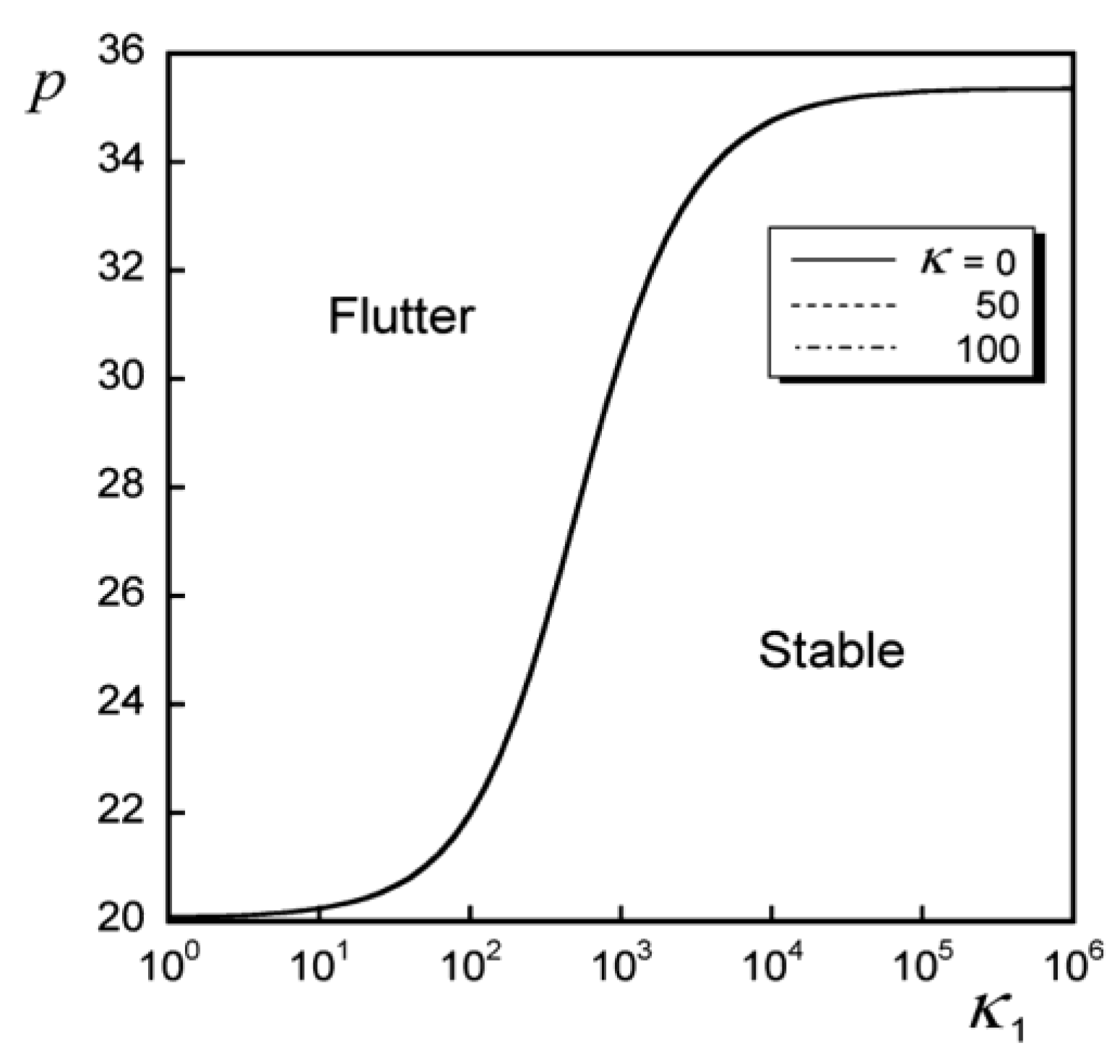
Figure 4 shows the critical follower force value according to the size of the intermediate support spring stiffness, k₁, when the elastic foundation parameter is k = 0, 50, 100 and the position of the intermediate support point is ${\xi }_1$ = 0.3. What can be seen from this figure is that, regardless of the sizes of k and k₁, only flutter-type instability occurs, and the critical value increases sharply when k₁ ranges from 10¹ to 10⁶.

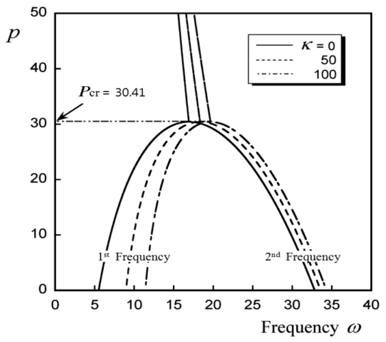
Figure 5 shows the first and second natural frequencies according to the change in the following force for the elastic foundation parameters are k = 0, 50, 100 when the intermediate support point position is ${\xi }_1$ = 0.3 and the intermediate support spring stiffness is k₁ = 10³. In this figure, flutter-type instability occurs where the first and second natural frequencies match, the critical flutter value at which flutter occurs is $p_{cr}=30.41$, and as the value of the elastic basis parameter k increases, the natural frequency value increases. However, it can be seen that there is no change in the critical flutter value.

Figure 6 shows the critical follower force value according to the size of the intermediate support spring stiffness, k1, when the elastic foundation parameters are k = 0, 50, 100 and the position of the intermediate support point is ${\mathsf{\xi }}_1$ = 0.2. When k = 0, flutter-type instability occurs in the section where k₁ ≤ 47.77, and as the value of k₁ increases, the critical follower force value increases rapidly. At k₁ = 47.77, there is a transition from flutter-type instability to divergence-type instability, and in the section of k₁ ≥ 47.77, only divergence-type instability occurs, and as the value of k1 increases, the critical follower force value decreases rapidly. In the case of k = 50, 100, it can be seen that there is a transition from flutter-type instability to divergence-type instability at k₁ = 55.29 and 64.88, respectively.

In Figure 7, in order to explain in more detail the process of transition from flutter-type instability to divergence-type instability, the position of the intermediate support point was calculated according to the change in the value of the following force when ${\xi }_1$ = 0.510, 0.515, 0.520, 0.525. It shows changes in the first and second natural frequency values. In the case of ${\xi }_1$ = 0.510, flutter-type instability, where the first and second natural frequencies match, occurs at p_cr = 36.48, and in the case of ${\xi }_1$ = 0.515, flutter-type instability occurs at p_cr = 41.67. The section where the first and second natural frequencies matched became shorter than when ${\xi }_1$ = 0.510, and the critical value at which flutter occurred increased. Divergence-type instability occurs at p_cr = 37.01, where the first natural frequency of ${\xi }_1$= 0.520 becomes 0, indicating that there has been a transition from flutter-type instability to divergence-type instability. In the case of ${\xi }_1$ = 0.525, divergence-type instability occurs at p_cr = 32.91, where the first natural frequency becomes 0, and the critical value at which divergence occurs is reduced compared to the case of ${\xi }_1$ = 0.520.

Figure 8 shows the instability type and critical follower force value according to the change in the position of the intermediate support point when the elastic foundation parameters are k = 0, 50, 100 and $\mathsf{\gamma }$ = 0.001 and the intermediate support spring stiffness, k₁ = 10⁶. In this figure, flutter-type instability occurs in the section where the position of the middle support point is ${\xi }_1$ ≤ 0.498, and the critical follower force value increases rapidly at ${\xi }_1$ = 0.499, resulting in a transition from flutter-type instability to divergence-type instability. In the range of ${\xi }_1$≥ 0.498, divergence-type instability occurs. Also, what can be seen from this figure is that, in the flutter section, there is a constant critical follower force value regardless of the value of the elastic basis parameter, and as the elastic support moves from the fixed end to the center (0 → 0.498), the critical follower force value increases. And in the divergence section, as the value of the elastic foundation parameter, k, increases, the critical follower force value increases, and as the elastic support moves from the center to the free-end direction (0.499 → 1), the critical follower force value decreases.

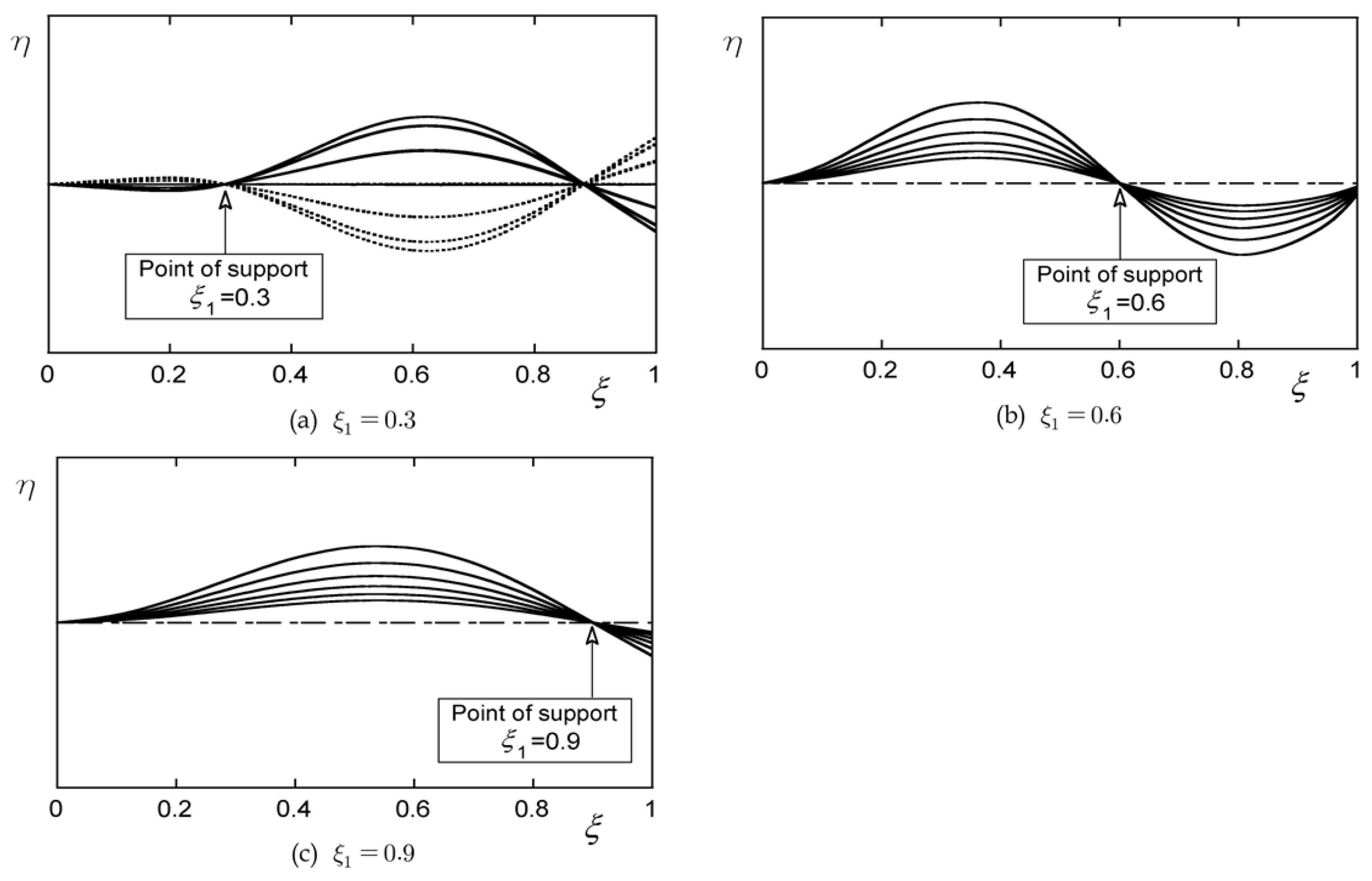
Figure 9 shows the instability mode shapes in each instability region (${\xi }_1$ = 0.3, 0.6, 0.9).

Figure 9a shows the instability mode shape when there is an intermediate support at the position of ${\xi }_1$ = 0.3. In this picture, it has a flutter-type unstable mode shape and is a third mode with two nodes.

Figure 9b shows the unstable mode shape when there is an intermediate support at the position of ${\xi }_1$ = 0.6, and it has a divergence-type unstable mode shape with upper and lower amplitudes based on the point of ${\xi }_1$ = 0.6.

When there is an intermediate support at the position of ${\xi }_1$ = 0.9, as shown in Figure 9c, it has a divergence-type instability mode shape with upper and lower amplitudes based on the point of ${\xi }_1$ = 0.9. Therefore, in Figure 9, it can be seen that the unstable mode shape and the order of the mode are different depending on the location of the intermediate support point.

Through the above analysis results, it was found that structural instability transitions near the center of the beam. Although there is no change in the critical value (p_cr) according to the number of finite-element divisions, the calculation was performed by dividing the finite elements into 40 to perform a detailed analysis of changes according to the intermediate support position (ξ₁). The change in the critical value of the follower force in the section where structural instability transitions was confirmed, and the number of finite-element divisions was increased to obtain detailed analysis values.

Figure 10a shows the results of the analysis performed using the range ξ₁ = 0.4~0.6 (pos) and the values of k₁ = 10⁶ (ssp) and k = 0 (fsp). It was confirmed that the intermediate support’s vibration divergence occurred as k₁ moved from 0.4 to 0.6. Figure 10b shows the results of the analysis performed using the range ξ₁ = 0.4~0.6 (pos) and the values of k₁ = 10⁶ (ssp) and k = 150 (fsp). It was confirmed that the intermediate support’s vibration divergence occurred as k₁ moved from 0.4 to 0.6. As shown in Figure 10a,b, the flutter critical value is the same as k changes, but when vibration diverges, the critical value increases further. Here, pos(x): represents the position ratio from the fixed end, ssp(x): represents the dimensionless parameter of the elastic support end, and fsp(x): represents the dimensionless parameter of the elastic support member.

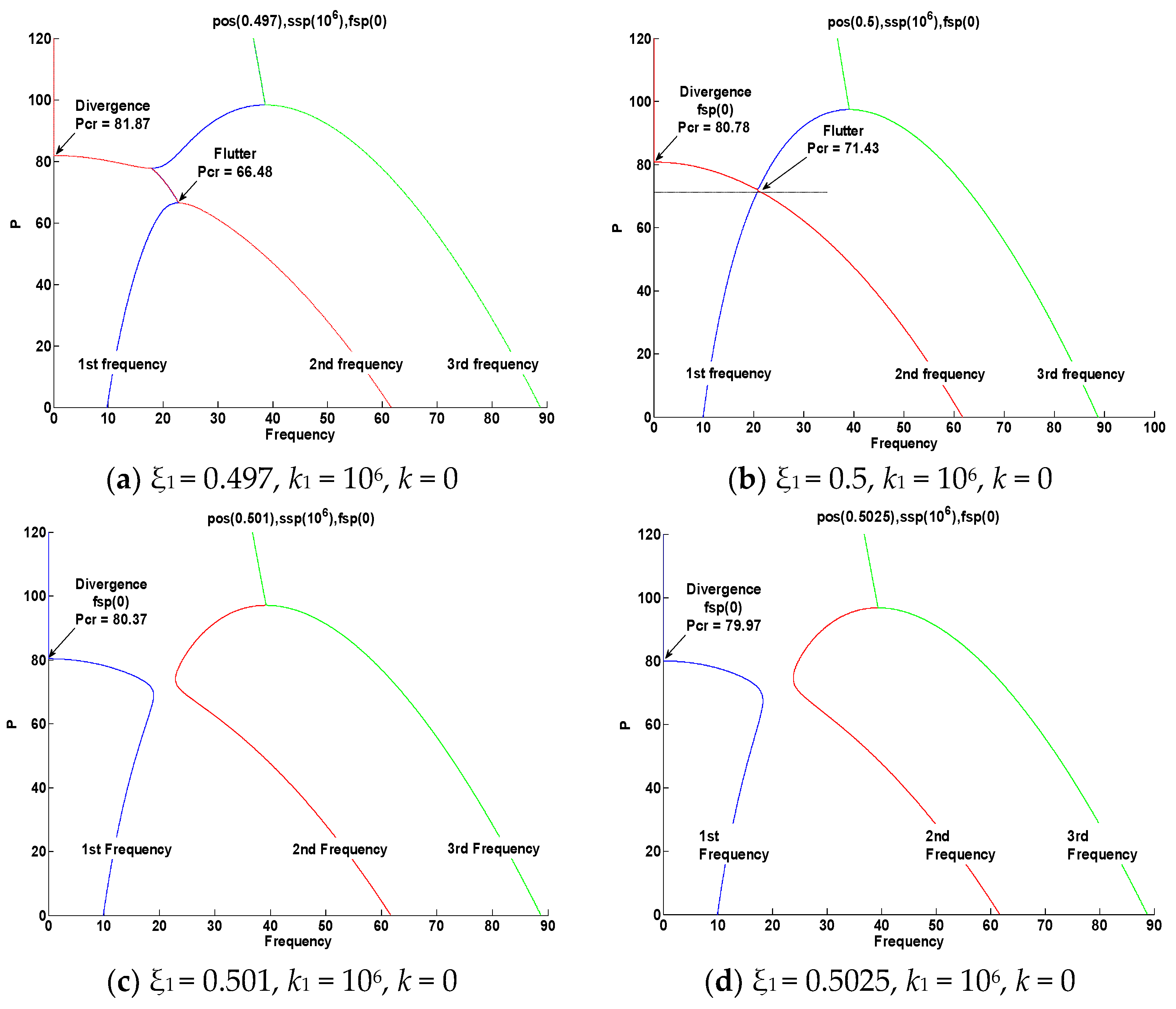
Figure 11 shows the process in which the intermediate elastic support transitions (flutter → divergence) according to the change in position (ξ₁). The critical value (p_cr) is in the form of flutter when the position of the intermediate support (k₁) increases from 0.497 → 0.525. It was confirmed that the critical value (p_cr) in the form of divergence decreased after the transition while rising.

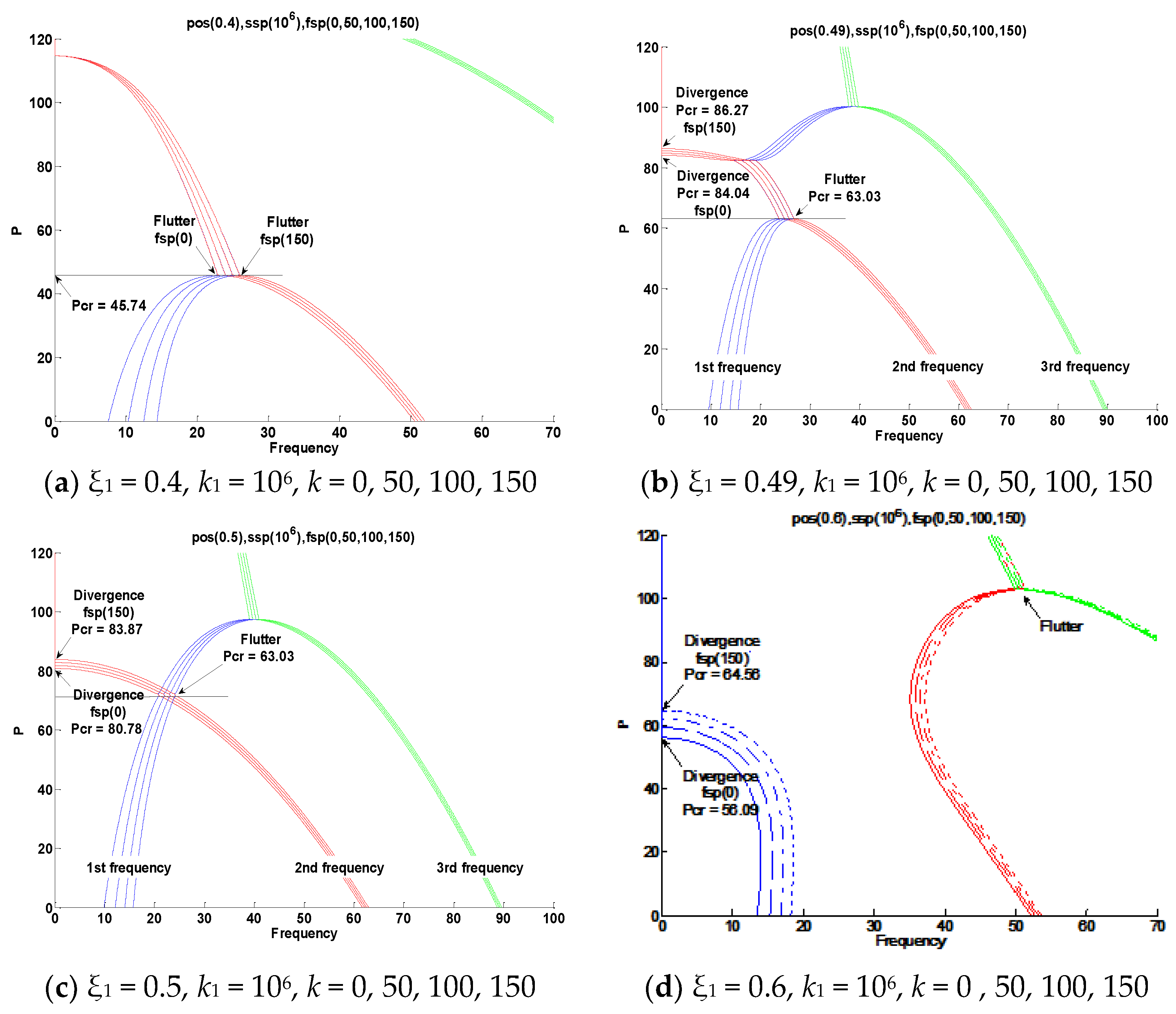
Figure 12 shows the change in location of the concentrated elastic support (ξ₁) and the increase in the elasticity value (k) of the distributed elastic support. The instability characteristics (flutter → divergence) changed according to the position change (ξ₁), the critical value (p_cr) was the same according to the change in value in the case of flutter-type instability, and the value changed in the case of divergence-type instability. Accordingly, the critical value (p_cr) increased. At this time, as the k value increased, each natural frequency increased. In the process of transition (flutter → divergence), Figure 12a shows instability in the form of flutter where the first and second natural frequencies meet. However, as the position change (ξ₁) increases, as shown in Figure 12b,c, instability in the form of flutter is followed by instability in the form of divergence due to secondary natural vibrations. Additionally, in Figure 12d, it was confirmed that instability in the form of divergence appears by the first natural frequency.

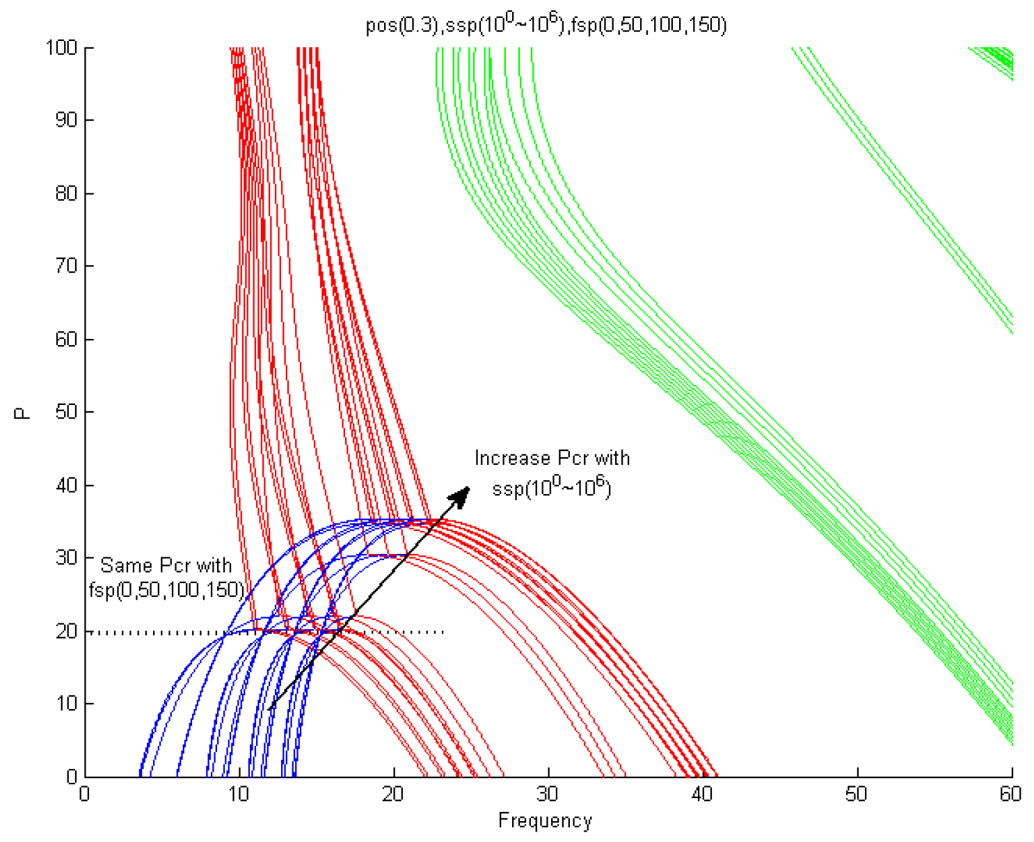
Figure 13 shows an analysis performed according to the increase in elasticity values of k₁ and k in the section ξ₁ = 0.3 (pos). For k₁, the values k₁ = 10⁰, 10¹, 10², 10³, 10⁴, 10⁵, 10⁶ (ssp) were applied step by step, and k was the result of the analysis by applying the values k = 0, 50, 100, and 150 (fsp). It was confirmed that as the elastic modulus of k₁ increased in the intermediate support section, the critical follower force value (p_cr) and the natural frequency increased. In addition, it was confirmed that as the elastic modulus of k increases, the critical follower force value (p_cr) remains unchanged and only the natural frequency increases.

Through this conclusion, as shown in Figure 12, it was confirmed that the natural frequency of the beam structure placed on an elastic foundation increases only as the elastic modulus (k) increases, and the critical value (p_cr) when unstable in the form of flutter is the same. It was confirmed that the critical value (p_cr) increases when instability occurs in the form of divergence.

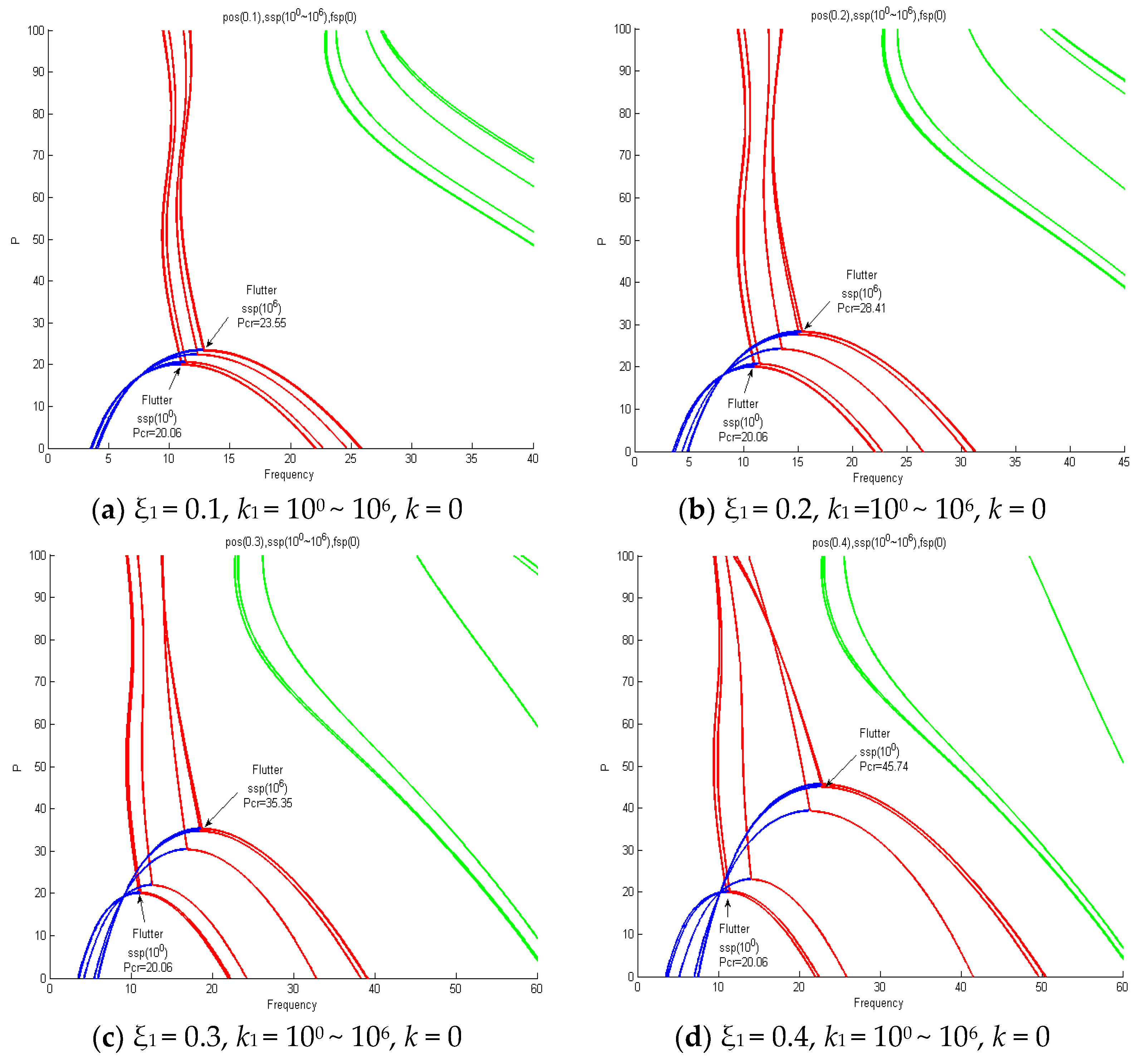
Figure 14 shows the change in critical value according to the change in the intermediate elastic support position (ξ₁) and the elastic support value (k₁). In the section where the ξ₁ value increases from 0.1 → 0.4 (pos), instability in the form of flutter was shown. In addition, it was confirmed that when the intermediate elastic support value increased to k₁ = 10⁰, 10¹, 10², 10³, 10⁴, 10⁵, 10⁶, the critical value (p_cr) and the natural frequency increased due to instability in the form of flutter. At this time, it was confirmed that the critical value (p_cr) increased rapidly at k₁ = 10², 10³, 10⁴ and that there was no change in the critical value depending on the value of k. When k₁ = 10⁰, the critical value according to the change in the intermediate elastic support position (ξ₁) was the same as p_cr = 20.06.

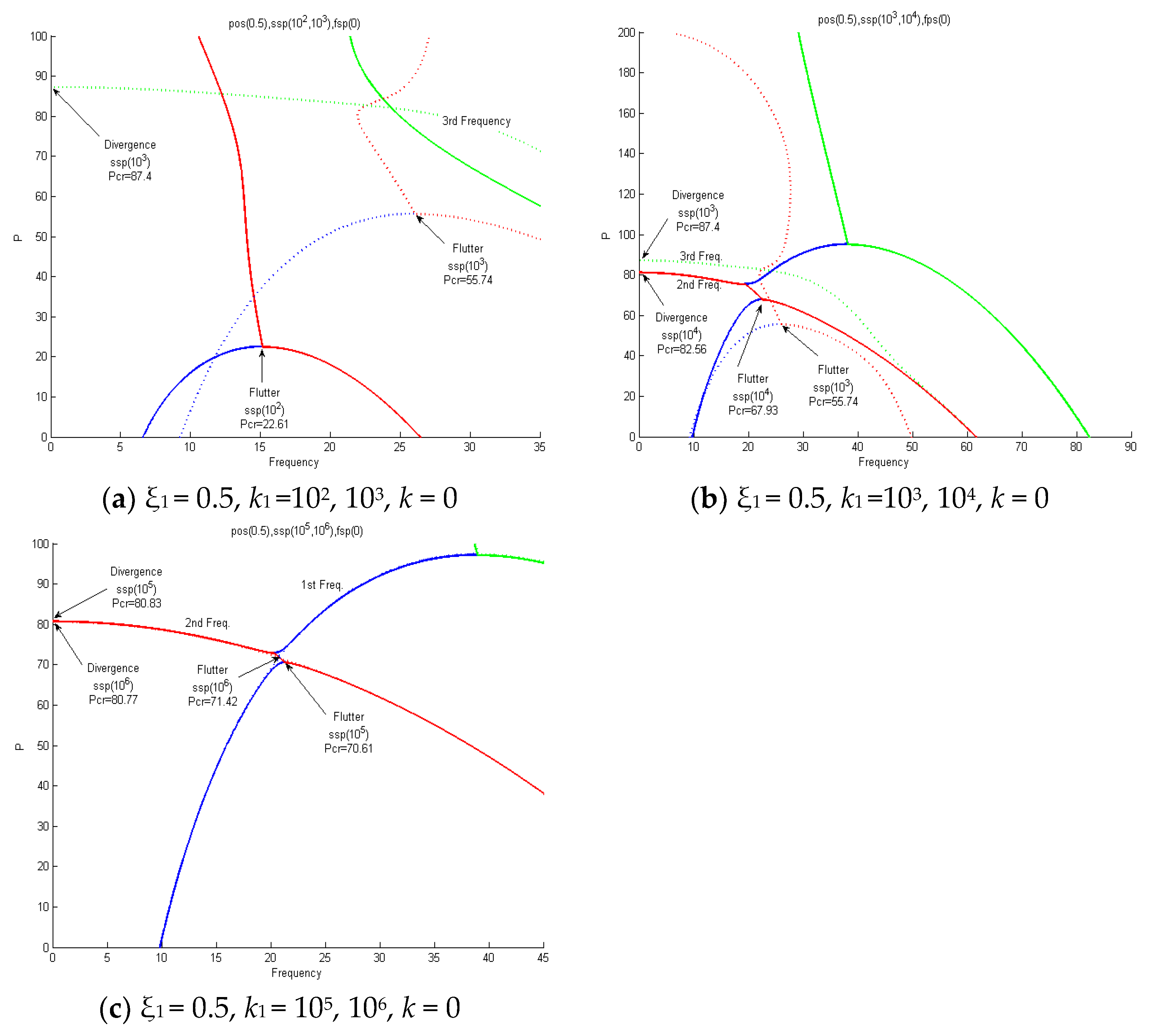
Figure 15 shows an analysis performed according to the elasticity value increase k₁ = 10², 10³, 10⁴, 10⁵, 10⁶ (ssp) in the ξ₁ = 0.5 (pos) section. Figure 15a applies the values of k₁ = 10² and 10³, and when k₁ = 10² increases from k₁ = 10³, the critical value increases from p_cr = 22.31 to p_cr = 55.74 due to instability in the form of flutter. When k₁ = 10³, the first and second natural vibrations met and flutter instability occurred. Then, at p_cr = 87.4, instability in the form of divergence appeared due to the third natural vibration. Figure 15b applies the values of k₁ = 10³ and 10⁴, and when increasing from k₁ = 10³ to k₁ = 10⁴, the critical value increased from p_cr = 55.74 to p_cr = 67.93 due to instability in the form of flutter. When k₁ = 10⁴, the first and second natural vibrations met and flutter instability occurred. Then, at p_cr = 82.56, instability in the form of divergence appeared due to the second natural vibration. In Figure 15b, k₁ = 10³ diverged by the third natural vibration, and k₁ = 10⁴ diverged by the second natural vibration. It was confirmed that when increasing from k₁ = 10³ to k₁ = 10⁴, the flutter critical value increased, but the divergence critical value after flutter decreased from p_cr = 87.4 to p_cr = 82.56. Figure 15c applies the values of k₁ = 10⁵ and 10⁶, and when increasing from k₁ = 10⁵ to k₁ = 10⁶, the critical value increased from p_cr = 70.61 to p_cr = 71.42 due to instability in the form of flutter. When k₁ = 10⁵, 10⁶, the first and second natural vibrations met and flutter instability occurred, and then instability in the form of divergence appeared due to the secondary natural vibrations at p_cr = 80.83 and p_cr = 80.77.

Figure 16 shows an analysis performed according to the increase in the elasticity value of k₁ (ssp) (k₁ = 10⁰, 10², 10³, 10⁴) in the ξ₁ = 0.55, ξ₁ = 0.6, ξ₁ = 0.7, ξ₁ = 0.9 (pos) section. Figure 16a shows flutter-type instability at ξ₁ = 0.55 and k₁ = 10², with a critical value of p_cr = 21.17. At ξ₁ = 0.55, k₁ = 10³, the first and second natural vibrations did not meet, but at p_cr = 49.83, the second and third natural vibrations met, showing instability in the form of flutter. Additionally, the first natural vibration showed divergence at p_cr = 71.34. Figure 16b shows flutter-type instability at ξ₁ = 0.6 and k₁ = 10², with a critical value of p_cr = 19.06. Unlike the flutter-type critical value at ξ₁ = 0.55, k₁ = 10² and the flutter-type critical value at ξ₁ = 0.6, k₁ = 10², which increased with k₁, the concentrated elastic support position (ξ₁) showed that the critical value decreased even as k₁ increased after ξ₁ = 0.55. At ξ₁ = 0.6 and k₁ = 10³, instability in the form of divergence first appeared at p_cr = 58.62. Figure 16c shows the same characteristics as Figure 16b, but the overall critical value has decreased. Figure 16d shows that the critical value of the flutter type decreased after ξ₁ = 0.55 at k₁ = 10², and then the first natural vibration showed instability in the form of divergence at p_cr = 28.76 at ξ₁ = 0.9.

4. Conclusions

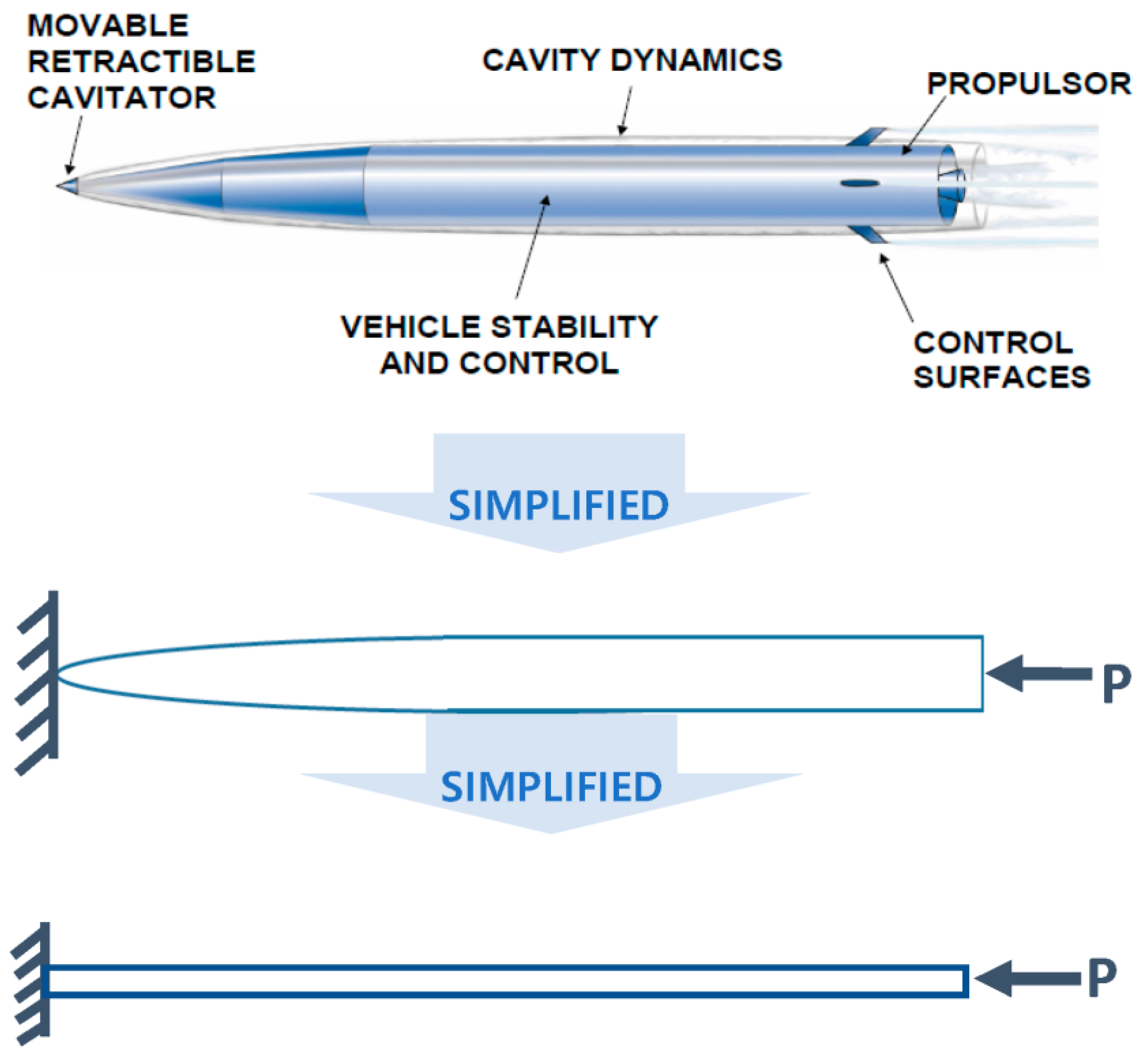
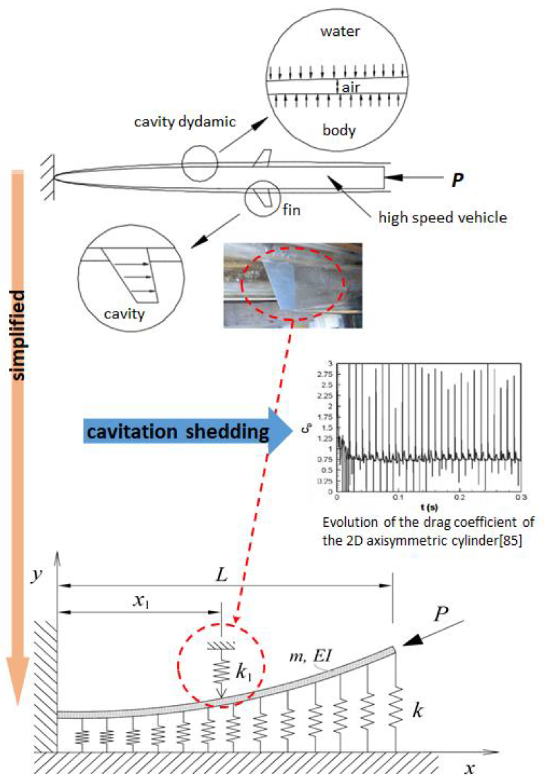
In this study, in order to analyze the structural instability characteristics of underwater high-speed vehicles, an underwater high-speed vehicle receiving propulsion at high speed was simplified into a cantilever-type model receiving driven force. In addition, the effect of the lumped mass that appears in the actual model was simplified to an intermediate support effect, and the effect of the change in the location of the lumped mass and the size of the lumped mass on structural stability was numerically analyzed. As a result of the numerical analysis, the parameters that affect the flutter-type instability, which is the dynamic instability of underwater high-speed moving objects, are the size and location of the concentrated mass, that is, the dimensionless elastic modulus (κ₁) and the location (ξ₁) of the intermediate support and the internal damping (γ). There are three parameters. On the other hand, there are four parameters that affect divergence-type instability, which is static instability: κ₁, ξ₁, γ, and the dimensionless coefficient (κ) of the elastic support.

In this study, we focused on the effect of three parameters, namely, κ₁, ξ₁, and κ, excluding γ, on the instability of underwater high-speed vehicles and obtained the following results.

First, as shown in Figure 6, as the size of the concentrated mass, that is, κ₁, increases, the instability characteristic transitions from flutter-type instability to divergence-type instability. Additionally, in the region of κ₁ that is smaller than κ₁ (κ_cr), where the transition occurs, p_cr is constant, regardless of κ, whereas in the region where κ₁ > κ_cr, p_cr changes depending on κ.

Second, as shown in Figure 8, when the internal damping of the beam is negligibly small, a transition from flutter-type instability to divergence-type instability occurs at ξ₁ = 0.499. Additionally, in the section where flutter-type instability occurs, p_cr is constant, regardless of κ, while in the section where divergence instability occurs, p_cr also increases as κ increases.

The main results obtained above are summarized as follows. The instability of a cantilever placed on an elastic foundation subjected to a follower force is divided into flutter-type instability and divergence-type instability areas depending on the elastic modulus and the location of the intermediate support. It can be seen that flutter-type instability appears toward the fixed end and that divergence-type instability appears toward the free end, around the center (L/2) of the beam. In addition, it is relatively stable as you move toward the center (L/2) of the beam, flutter-type instability is likely to appear as you move from the center (L/2) of the beam toward the fixed end, and divergence-type instability is likely to appear as you move toward the free end.

Therefore, when a large following force is applied to an actual underwater high-speed vehicle, instability appears as the center of gravity moves from the center to both ends, so this should be taken into consideration when designing, and it can be used as a guideline for controlling instability when designing a structure subject to a following force. If a mechanism that can generate a supercavity at a specific location is introduced, the entire moving body can be formed into a supercavity even with relatively small thrust. And in the case of beams with concentrated mass at the ends, the critical value is relatively high, so stability can be secured by the following force. Therefore, when a large following force is applied to an actual underwater high-speed vehicle, instability appears as the center of gravity moves from the center to both ends; so, unlike missiles that have the same aerodynamic characteristics, the position of the control pin is considered from the center toward the bow. Thus, it was clear that the design was necessary. It can also be used as a control guideline for instability when designing structures subject to driving force.

References

1. Ahn, S.S. An Integrated Approach to the Design of Supercavitating Underwater Vehicles. Ph.D. Thesis, School of Aerospace Engineering, Georgia Institute of Technology, Atlanta, GA, USA, 2007. [Google Scholar]
2. Scientific American, Inc. Scientific American Special Online Issue—The Science of War: Weapons; Scientific American, Inc.: New York, NY, USA, 2002. [Google Scholar]
3. John, L.S.; Hess, R.W.; Watkins, C.E. Analytical and Experimental Investigation of Flutter and Divergence of Sping-Mounted Cone Configurations at Supersonic Speeds; NASA Technical Note, D1021; NASA: Washington, DC, USA, 1962.
4. Savchenko, Y.N. Experimental Investigation of Supercavitating Motion of Bodies; Ukrainian National Academy of Sciences—Institute of Hydromechanics: Kyiv, Ukraine, 2001. [Google Scholar]
5. Kirschner, I.N.; Kring, D.C.; Stokes, A.W.; Fine, N.E.; Uhlman, J.S., Jr. Control Strategies for Supercavitating Vehicles. J. Vib. Control 2002, 8, 219–242. [Google Scholar] [CrossRef]
6. Kim, J.H. A Robust Impulsive Control Strategy of Supercavitating Vehicles in Changing Systems. Appl. Sci. 2018, 8, 2355. [Google Scholar] [CrossRef]
7. Semenenko, V.; Naumova, O. Some ways of hydrodynamic fin application for underwater supercavitating vehicles. Hydrodyn. Acoust. 2019, 1, 355–371. [Google Scholar] [CrossRef]
8. Beck, M. Die Knicklast des Einseitig Eingespannten Tangential Gedrukten Stabes. ZAMP 1952, 3, 225–228. [Google Scholar]
9. Sugiyama, Y.; Langthjem, M.A.; Ryu, B.J. Realistic Follower forces. J. Sound Vib. 1999, 225, 779–782. [Google Scholar] [CrossRef]
10. Rao, G.V.; Raju, K.K. Stability of Tapered Cantilever Columns with an Elastic Foundation Subjected to a Concentrated Follower Force at the Free End. J. Sound Vib. 1982, 81, 147–151. [Google Scholar] [CrossRef]
Figure 1. Real vehicle in cavitation condition and simplified model.
Aerospace 10 00916 g001
Figure 2. Beck’s beam on an elastic foundation with an intermediate support.
Aerospace 10 00916 g002
Figure 3. Finite element model of beam.
Aerospace 10 00916 g003
Figure 4. Critical follower force as a function of the intermediate support when k1 = 100 to 106.
Aerospace 10 00916 g004
Figure 5. First and second frequency curves for follower forces when the stiffness of elastic foundation k = 0, 50, 100; γ = 0.0; and ξ 1 = 0.3.
Aerospace 10 00916 g005
Figure 6. Critical follow force curves for the parameter of intermediate elastic support k1 when k = 0, 50, 100; γ = 0.0; and ξ 1 = 0.2.
Aerospace 10 00916 g006
Figure 7. First, second, and third frequency curves for follower forces when k = 0 and γ = 0.0.
Aerospace 10 00916 g007
Figure 8. First, second, and third frequency curves for follower forces when k = 0, 50, 100 and γ = 0.001.
Aerospace 10 00916 g008
Figure 9. Unstable modes for one cycle of oscillation at the location of intermediate support, ξ 1 = 0.3, 0.6, 0.9, when γ = 0.0.
Aerospace 10 00916 g009
Figure 10. First, second, and third frequency curves for follower forces when ξ1 = 0.4~0.6, k1 = 106, and k = 0, 150.
Aerospace 10 00916 g010
Figure 11. First, second, and third frequency curves for follower forces when ξ1 = 0.497, 0.5, 0.501, 0.5025; k1 = 106; and k = 0.
Aerospace 10 00916 g011
Figure 12. First, second, and third frequency curves for follower forces when ξ1 = 0.4, 0.49, 0.5, 0.6; k1 = 106; and k = 0, 50, 100, 150.
Aerospace 10 00916 g012
Figure 13. First, second, and third frequency curves for follower forces when ξ1 = 0.3; k1 = 100~106; and k = 0, 50, 100, 150.
Aerospace 10 00916 g013
Figure 14. First, second, and third frequency curves for follower forces when ξ1 = 0.1~0.4, k1 = 100~106, and k = 0.
Aerospace 10 00916 g014
Figure 15. First, second, and third frequency curves for follower forces when ξ1 = 0.5; k1 = 102, 103, 104, 105, 106; and k = 0.
Aerospace 10 00916 g015
Figure 16. First, second, and third frequency curves for follower forces when ξ1 = 0.55, 0.6, 0.7, 0.9 and k1 = 100, 102, 103, 104.
Aerospace 10 00916 g016
Disclaimer/Publisher’s Note: The statements, opinions and data contained in all publications are solely those of the individual author(s) and contributor(s) and not of MDPI and/or the editor(s). MDPI and/or the editor(s) disclaim responsibility for any injury to people or property resulting from any ideas, methods, instructions or products referred to in the content.