Modeling and Application of Out-of-Cabin and Extra-Vehicular Dynamics of Airdrop System Based on Kane Equation

Abstract

The application of the Kane equation in analyzing airdrop dynamics problems is rare. The main objective of this paper is to apply the Kane equation dynamics model to the analysis of the status continuity problem during the out-of-cabin process and the line sail phenomenon during the extra-vehicular process. In the out-of-cabin process, an analysis of off-aircraft security and traction ratio impact was conducted. Furthermore, the BP neural network model was trained to predict the status transition of the payload for a multiple airdrop mission. In the extra-vehicular process, the spring network method was used together with the Kane equation to analyze the form and overload of the parachute line. The modeling avoids complex equations and derivations. The results suggest significant potential applications of the Kane equation in precision airdrop missions during out-of-cabin and extra-vehicular processes without heavy reliance on experimental data.

1. Introduction

Simulation methods based on Newton’s equations have been extensively applied in the field of precision airdrops in recent years [1]. Currently, wind tunnel tests and airdrop experiments serve as crucial and reliable sources for the acquisition of the dynamic properties and data from airdrops. However, due to the high cost of these methods, simulation models for airdrops are gradually gaining prominence as an area of research focus.

The key challenges in simulating the dynamics model of airdrops include equation selection, system modeling, and solution methods. In terms of equation selection, the classical Newton’s equations are predominantly employed as they are suitable for modeling and analyzing various specific rigid body systems. Within this field of research related to Newton’s equations, particular attention is given to studying degrees of freedom and motion constraints within rigid body systems. From the 1980s to the 2000s, there was an increase in the number of degrees of freedom from the initial three degrees [2,3] to six degrees [4,5,6], eight degrees [7,8,9], nine degrees [10,11], ten degrees [12,13], and twelve degrees [14]; recently, this increase has reached fifteen degrees due to more bodies in the aircrafts [15].

Although the Kane equation has received relatively less attention in the field of airdrops, its simplicity and versatility in dealing with scalable multibody systems have been demonstrated to be superior to Newton’s equations. In 1989, T. Jia et al. [16] introduced the concept of the gap function to convert force constraints from the inequality form to the equation form when studying impact forces in multibody systems. S. Kemal Ider et al. [17] further extended this work by investigating constrained control forces in multi-systems and exploring the introduction of control forces in general directions. In 2007, R. Beck et al. [18] applied the Kane equation to stepless transmissions and clutches in automobiles and compared it with the standard PI control. Q. Hu et al. [19] conducted research on the automatic generation of equations of motion with varying degrees of freedom using computer programming, while enhancing the Kane equation’s motion constraints and validating the results. S. Šalinić et al. [20] developed a hydraulic excavator dynamics model utilizing the Kane equation to examine the topographical effects caused by stochasticity. D. Chowdhury et al. [21] studied modifications of the Kane equation parameters caused by the effect of spin currents. J.Y. Liu et al. [22] developed a suppression system model for non-powered propulsion vessels, employing Kane equations to explore various influences. R.S. Pal et al. [23] characterized helicopter underslung dynamics using the Kane equation, while K.K. Sharma et al. [24] linearized helicopter underslung dynamics models to discuss lateral load dynamics.

In contrast to the use of Lagrange equations, the Kane equation has demonstrated remarkable simplicity and versatility by being applicable to both complete and incomplete systems. While the Kane equation has been extensively applied and enhanced in various fields, its application in airdrop system dynamics model development remains relatively unexplored. However, given the complexity and modularity of typical multibody structures in airdrop systems, the Kane equation is well suited for such applications.

The modeling of the interaction between the load and the cargo bay during the in-cabin process of an airdrop, and ensuring a smooth and safe departure of the payload are crucial issues. The interaction between the load and the cargo bay significantly affects the post-departure attitude of the payload, and the subsequent landing accuracy, and requires high-precision dynamic modeling. Bagdonovich et al. [25] studied different departure processes and concluded that departure time is a key factor affecting landing accuracy for low-altitude airdrop systems. NASA-JSC [26,27,28] developed the DSS with a spring model to simulate the contact constraint between the ramp and load; however, the parameter variation still needs to be determined by experimental data. Irvin Aerospace’s DCLDYN [29] also contained an aircraft–load interaction model during an extra-vehicular process, but lacked a clear demonstration of a specific model. K. P et al. [30] developed a simulation model that provided a separate status, but it lacked generality, making transferability across different airdrop systems difficult.

In most simulation model studies, the results lack output continuity status decision making and thus lack automatic identification capabilities. This characteristic has been extensively explored in the field of artificial intelligence, particularly with regard to neural networks (NNs), which are well suited for addressing this issue and have relevant applications in the airdrop field. Compared to previous methods, deep learning methods [31] and backpropagation neural network (BPNN) approaches avoid complex model derivation and significantly reduce modeling difficulty [32]. L.W. Hu et al. [33], Kai Li et al. [34], and MGD Giorgi et al. [35] focused on enhancing the reduced-order model (ROM) in computational fluid dynamics (CFD) by utilizing prediction results from convolutional neural network (CNN) and long short-term memory (LSTM) models to replace experimental data for the obtainment of aerodynamic information. The inherent characteristics of the BPNN offer significant advantages in model classification and pattern recognition [36], making it suitable for the analysis of the disordered categorical variables present in the status data discussed within this paper. Furthermore, since the amount of status data is smaller than that of the dynamic data during an airdrop process, the BPNN can meet the computational requirements.

During the extra-vehicular phase, the parachute line straightening process is critical and can be divided into two types: pulling the parachute canopy first or pulling the parachute line first [37]. When the line is pulled first, it can cause the line sail phenomenon, also called the line bowing or fish hooking phenomenon, as shown in Figure 1. It can have an adverse effects on the inflation process of the main parachute, and Moog et al. [38], Purvis et al. [39,40], Johnson et al. [41], Peterson et al. [42], and Maydew et al. [43] have made detailed studies of it. They discussed six situations: prolonged opening time, collision between the parachute bag and the canopy, high cord straightening force, asymmetric opening, wear of the canopy by the parachute bag, and unpredictable parachute inflation. However, recent researchers have mainly focused on simulating this phenomenon using a fluid–solid coupling method, which requires complex computational equipment, making it less applicable. There are few studies that use mechanical equations to model dynamic differential equations with simplified models. Through the use of the Kane equation mathematical model and the spring mesh physical model, the complex motion of the line is taken into account while the computational effort needed for the simulation analysis of the line sail phenomenon during straightening is reduced, resulting in more generalizable and robust results.

In this paper, the Kane equation is used for the dynamic models of the out-of-cabin process and the extra-vehicular process. The payload status transition problem in the out-of-cabin process and the prediction of the line sail phenomenon in the extra-vehicular process are studied. Additionally, the BP neural network is introduced in the out-of-cabin process, and its feasibility for the identification of payload status is proved. The spring network method is combined with the Kane equation in the modeling of the extra-vehicular process to predict the rope sail phenomenon accurately. The dynamic model results of the two processes reduce the reliance on experimental data and can provide an important reference for airdrop research.

2. Methods

In our earlier studies, the Kane equation method was verified through comparison with the results from Prakash [44], proving its great adaptiveness and accuracy for the dynamics. In this paper, the Kane equation is used in the out-of-cabin process and extra-vehicular process for the dynamic equations. In the out-of-cabin process, the Kane equation dynamic simulation results are used as training data, and the BP neural network is used to obtain a model trained for the prediction of the different status transitions of the payloads during multiple airdrop missions; this is called the status continuity issue. In the extra-vehicular process, the Kane equation is used to predict the line sail phenomenon together with the spring network method, which is a type of method that uses a system of discrete mass points.

2.1. Out-of-Cabin Process Dynamics

The interior of the transport aircraft cargo bay is modeled with appropriate simplification and is based on the relationship of structural position changes via multibody dynamics. The schematic diagram of the system’s rigid body connection and the imaginary topology of the multibody are shown in Figure 2, where the system’s degrees of freedom and part numbers have been indicated. In addition, the initial position of the payload inside the cabin affects the departure and drop point; so, the position of the payload and the physical parameters of each structure of the cargo bay are set according to the real aircraft data. The cargo bay is divided into horizontal and inclined sections, where the length of the horizontal section is $L_0=9.0 \mathrm{m}$, the inclination angle is ${\theta }_0=4°20\prime$, and the vertical height of the inclined section is $H_0=0.64 \mathrm{m}$.

A few assumptions and simplifications are used in the model:

(1)

Due to the symmetry of the system, only the displacement and pitch motion along the direction of flight and gravity are considered, i.e., the coordinate system is simplified to two dimensions;

(2)

The aircraft maintains a horizontal uniform velocity during the airdrop, and an angle of attack can exist;

(3)

No aerodynamic influence is considered when the load is moving inside the cabin;

(4)

Due to the long traction rope, the influence of the aircraft’s wake flow on the traction parachute and parachute rope characteristics is not considered.

The system is modeled using two-dimensional rigid body dynamics. The degrees of freedom are chosen to be 3. The generalized coordinates of the system are chosen to correspond to the spatial position of the load at 1 point on the imaginary rigid body 1, i.e., the center of mass position x,y and its attitude angle $\theta$. That is:

$$q={(x,y,\theta )}^T$$

(1)

Thus, the generalized velocity and the first-order derivative of the generalized coordinates are:

$$\dot{q}={(u_1,u_2,u_3)}^T={(\dot{x},\dot{y},\dot{\theta })}^T$$

(2)

Furthermore, the coordinate system uses the inertial system ($O_i{X}_i{Y}_i$) and the load solid coordinate system ($O_o{X}_o{Y}_o$). Its coordinate system transformation matrix is:

$$\left(\begin{array}{c}{x}_i\\ y_i\end{array}\right)=T_{io}\cdot \left(\begin{array}{c}{x}_o\\ y_o\end{array}\right)=\left(\begin{array}{cc}\cos \theta & -\sin \theta \\ \sin \theta & \cos \theta \end{array}\right)\cdot \left(\begin{array}{c}{x}_o\\ y_o\end{array}\right)$$

(3)

Next, the angular velocity, angular acceleration, velocity, and acceleration of each component of the system are determined. First, the angular velocity transformation matrix is needed to calculate the above quantities in the Kane equation:

$$H_{io}=\left(\begin{array}{ccc}\cos \theta & -\sin \theta & 0\\ \sin \theta & \cos \theta & 0\\ 0& 0& 1\end{array}\right)$$

(4)

The system includes coordinate origin point O and load node 1; so, the angular velocity of the system is:

$$w_1=H_{io}\cdot {(u_1,u_2,u_3)}^T=W_1{u}_1+W_2{u}_2+W_3{u}_3$$

(5)

The system velocity is given by:

$$v_1=H_{io}\cdot {(u_1,u_2,u_3)}^T+w_1\times H_{io}\cdot {(u_1,u_2,u_3)}^T$$

(6)

The system angular velocity is given by:

$${\alpha }_1={\dot{w}}_1$$

(7)

The system acceleration is given by:

$$a_1={\dot{v}}_1$$

(8)

The deflected velocity and deflected angular velocity are calculated from the dynamic quantities of the system:

$$\begin{array}{l}{v}_{i,q}={\left[\frac{\partial v_i}{\partial u_j}\right]}_{1\times 3}=\left(\begin{array}{ccc}\frac{\partial v_1}{\partial u_1}& \frac{\partial v_1}{\partial u_2}& \frac{\partial v_1}{\partial u_3}\end{array}\right)\\ w_{i,q}={\left[\frac{\partial w_i}{\partial u_j}\right]}_{1\times 3}=\left(\begin{array}{ccc}\frac{\partial w_1}{\partial u_1}& \frac{\partial w_1}{\partial u_2}& \frac{\partial w_1}{\partial u_3}\end{array}\right)\end{array}$$

(9)

where the subscripts denote the different nodes of the system structure, which are taken as 1, and j implies the different generalized coordinates.

All the forces of the system are summarized as generalized principal forces and generalized inertial forces and active moments:

$$\begin{array}{l}F=F_i{v}_{i,q}=F_i{\left[\frac{\partial v_i}{\partial u_j}\right]}_{1\times 3}\\ F^{*}=F_i^{*}{v}_{i,q}=-m_i{a}_i{\left[\frac{\partial v_i}{\partial u_j}\right]}_{1\times 3}\\ M=M_f+M_F+[I_i{\dot{w}}_i+w_i\times (I_i{w}_i)]w_{i,q}=(f\times \frac{h}{2})v_{i,q}-(F\times r)v_{i,q}+[I_i{\dot{w}}_i+w_i\times (I_i{w}_i)]w_{i,q}\end{array}$$

(10)

where $F_i$ is all the generalized principal forces on the nodes in the different systems, consisting of all the external forces on the system. $F_i^{*}$ is all the generalized inertial forces on the nodes within the different systems. The main dynamic forces at the nodes of the system consist of all the external forces to which the system is subjected, including the four categories $f,G,F,N$ namely the frictional forces to which the rigid structure $i$ is subjected, the gravitational forces, the support forces, and the tensile forces acting on the bottom side of the right endpoint. Only two contact relations, the line surface contact and face surface contact, need to be modeled separately for the main dynamic forces, as shown in Figure 3. If the payload and the cargo bay are separated entirely, only the support forces need to be erased.

In the state (a), the external force and the calculation method are:

$$\begin{array}{l}N=k_1(G\cos \theta -F\sin \theta -m_i{a}_f)\\ G=m_{i}g\\ f=\mu N\end{array}$$

(11)

where N is the support force, G is the gravitational force, m_i is the mass of the load, μ is the kinetic friction factor on the ground inside the cabin, F is the tension of the parachute rope acting on the lower right corner of the load, and the coefficient $k_1$ and acceleration $a_f$ are:

$$\begin{array}{l}{k}_1=1.0/(1.0+\frac{m_i}{I_i}(l^2+\frac{\mu lh}{2}))\\ a_f=[{(u_1,0,0)}^T\cdot \cos \theta +{(0,u_2,0)}^T\cdot \sin \delta +\dot{l}]\cdot {(0,0,u_3)}^T-\frac{\mathit{F}lr}{I_i}\end{array}$$

(12)

where h is the equivalent rectangular height of the load, l is the position vector between the contact point S and the midpoint of the bottom edge of the load, the vertical position vector r is from the center of mass C to the tension force, and the rotational inertia of the load I_i is with respect to the center of mass C.

In state (b), the external force and the calculation method are:

$$\begin{array}{l}N=G\\ G=m_{i}g\\ f=\mu N=\mu G\end{array}$$

(13)

At the same time, according to the constraint that the velocity of the point S is zero in the direction of the support force, the formulae for the calculation of various force matrices can be obtained. In addition, the change in angular velocity is solved for the deflected angular velocity according to the momentum moment theorem:

$$\begin{array}{l}{v}_{SN}=u_2\cos \delta -u_1\sin \delta -u_3\cdot r=0\\ {v^{\prime }}_{SN}=0\\ {v^{\prime }}_{Sf}-v_{Sf}=0\\ w^{\prime }=\{\begin{array}{l}(w-\frac{mr\cdot v_{CN}}{I_i})/(1-\frac{mr\cdot r}{I_i})\hspace{1em}\mathrm{other} \mathrm{states}\\ 0\hspace{1em}\hspace{1em}\hspace{1em}\hspace{1em}\hspace{1em}\hspace{1em}\hspace{1em}\mathrm{line} \mathrm{to} \mathrm{surface} \mathrm{state}\hspace{1em}\end{array}\end{array}$$

(14)

where $v_{SN}^{\prime }$ and $v_{Sf}^{\prime }$ denote the velocity components of the contact point S in the support and friction directions, respectively, at the next moment after the collision, and $v_{CN}$ are the components of the center-of-mass velocity in the support direction. The above three quantities are the same as the system velocity expressions, and all of them are expressed in generalized coordinates in the calculation process.

The stochastic wind field is added to the stochasticity factor part, which includes both steady $v_{gust}$ and random $v_{rand}$ wind components. The gust model proposed by NASA [45] is improved to simulate the directional steady wind, as follows:

$$v_{gust}=\{\begin{array}{l}0\hspace{0.17em}\hspace{0.17em}\hspace{0.17em}\hspace{0.17em}\hspace{0.17em}\hspace{0.17em}\hspace{0.17em}\hspace{0.17em}\hspace{0.17em}\hspace{0.17em}\hspace{0.17em}\hspace{0.17em}\hspace{0.17em}\hspace{0.17em}\hspace{0.17em}\hspace{0.17em}\hspace{0.17em}\hspace{0.17em}\hspace{0.17em}\hspace{0.17em}\hspace{0.17em}\hspace{0.17em}\hspace{0.17em}\hspace{0.17em}\hspace{0.17em}\hspace{0.17em},0\hspace{0.17em}<h\le H/4\\ \frac{v_{gust}^{\max }}{2}\left(1-\cos \left(\frac{(h-H/4)\pi }{H}\right)\right),H/4<h\le H/2\\ v_{gust}^{\max }\hspace{0.17em}\hspace{0.17em}\hspace{0.17em}\hspace{0.17em}\hspace{0.17em}\hspace{0.17em}\hspace{0.17em}\hspace{0.17em}\hspace{0.17em}\hspace{0.17em}\hspace{0.17em}\hspace{0.17em}\hspace{0.17em}\hspace{0.17em}\hspace{0.17em}\hspace{0.17em}\hspace{0.17em}\hspace{0.17em}\hspace{0.17em}\hspace{0.17em}\hspace{0.17em}\hspace{0.17em},H/2<h\le 3H/4\\ \frac{v_{gust}^{\max }}{2}\left(1-\cos \left(\frac{(h-3H/4)\pi }{H}\right)\right),3H/4<h<H\end{array}$$

(15)

where $v_{gust}^{\max }$ denotes the velocity maximum of the directional steady-state wind; and h and H are the instantaneous altitude and the total altitude of the airdrop, respectively. The random winds are stored in a two-dimensional array $v_{rand}=[\begin{array}{cc}{v}_r& d_r\end{array}]$, where $v_r$ is the wind amplitude introduced by generating small-amplitude time-varying random numbers (below 1 m/s), and $d_r$ is the wind direction expressed in terms of Euler angles, which is also introduced by generating random numbers in the range (0° to 360°). The wind field is introduced into the equations by adding the steady and random wind vectors to the velocity term in the dynamic equations.

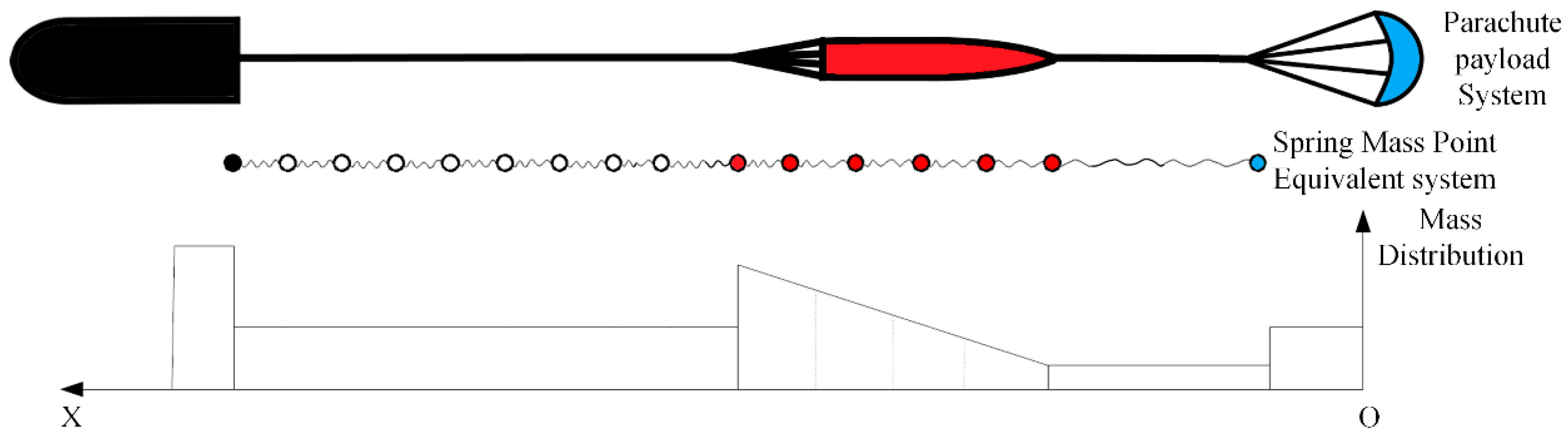
2.2. Extra-Vehicular Process Dynamics of the Line

The fabric aerodynamic deformation problem has a large theoretical difficulty. The model in the paper is discretized into a series of interconnected masses by the spring for the parachute line space curve and develops a spring network method unified form. It is appropriate to increase the discrete nodes. The model results get closer to the exact solution; at the same time, it can avoid excessive dependence on the moment constraints and also achieve partial decoupling. It has great advantages in solving the parachute line simulation problem. For the line sail phenomenon which may occur in the extra-vehicular phase, the spring network method is combined with the Kane equation to derive the dynamic model of the parachute line, and the results are obtained to solve the problem which was originally difficult to analyze via the Newtonian method. Additionally, the equations are more concise and easier to apply, with a simpler process.

To facilitate the analysis of the problem, the following assumptions are made:

(1)

The rotation of the cargo is not considered. The studies by Wang H. [46] show that its rotation only has an effect on the calculation results of its own attitude and has no effect on the line sail phenomenon generated on the connecting line.

(2)

There is no inflation of the main parachute during the straightening process, and it can be regarded as a one-dimensional object in space, similar to the parachute line, whose aerodynamic force is calculated in the same way as that of the parachute attachment line.

(3)

It is assumed that the angle of attack of the traction parachute is always zero in the straightening process.

(4)

The aerodynamic force acting on the parachute connecting line and the uninflated main parachute is calculated as a cylinder.

The parachute line system with N discrete points can be regarded as an ideal and complete constrained mass point system with one degree of freedom. Taking the generalized coordinates as $q_1,q_2,\dots ,q_n$, the vector diameter $r_i$ of every mass point $m_i$ in the mass point system can be expressed as a function of the generalized coordinates and time:

$${\mathbf{r}}_i={\mathbf{r}}_i\left(q_1,q_2,\dots ,q_n;t\right)$$

(16)

$F$ is the generalized principal force corresponding to the generalized coordinate $q_j$:

$$F={\displaystyle \sum _{i=1}^n{\mathbf{F}}_i\cdot \frac{\partial {\mathbf{r}}_i}{\partial q_j}}$$

(17)

$F_i$ is the principal force acting on m_i within the system, corresponding to the spring network model described earlier:

$$F_i={\displaystyle \sum _b{F}_{s,b}+F_{a,i}}$$

(18)

$F_{a,i}$ is the aerodynamic force acting in the control domain around the mass point, and $F_{s,b}$ is the force generated by the spring connected to the mass point, including both the elastic and damping components, which can be calculated by:

$$F_{s,b}=\left(E_b{A}_b{\epsilon }_b+B_b{\dot{\epsilon }}_b\right)\cdot \frac{\left(r_b-r_i\right)}{\left|r_b-r_i\right|}$$

(19)

where

$${\epsilon }_b=\frac{\left|r_b-r_i\right|-\left|r_{b,0}-r_{i,0}\right|}{\left|r_{b,0}-r_{i,0}\right|}$$

(20)

The derivative for time is obtained by:

$${\dot{\epsilon }}_b=\frac{\left(r_b-r_i\right)\cdot \left({\dot{r}}_b-{\dot{r}}_i\right)}{\left|r_b-r_i\right|\cdot \left|r_{b,0}-r_{i,0}\right|}$$

(21)

where $\left|r_{b,0}-r_{i,0}\right|$ denotes the length of the spring adjacent to the mass point in the absence of elastic tension; $E_b$ is the Young’s modulus of the adjacent spring; $A_b$ is the cross-sectional area of the spring; and $B_b$ is the damping factor of the adjacent spring.

In the Cartesian coordinate system, the vector diameter $r_i$ of the mass point can be expressed in coordinate components as:

$$r_i=q_{i,1}\cdot i+q_{i,2}\cdot j$$

(22)

The connecting line basically does not need to consider the frictional force during the pull-out process from the parachute bag, but for the uninflated main parachute, the frictional force needs to be considered, and this frictional force is basically constant during the pull-out process [47]. The frictional force is considered in the following way: for the nodes just pulled out, the direction of the frictional force should be the same as the direction of the spring elasticity between the unpulled nodes, and the frictional force is essentially acting equally on the unpulled nodes; so, there is:

$$F_{f,i}=f\cdot r$$

(23)

where r is the unit vector of the displacement vector from the node just pulled out to the node not pulled out, and $i$ is the number of the node just pulled out. For the unpulled nodes:

$$F_{f,j}=\frac{m_j\cdot f\cdot (-r)}{{\displaystyle \sum _j{m}_j}}$$

(24)

The meaning of the above equation is gained by dividing the frictional force on each unpulled node to ensure that the unpulled nodes move together.

According to assumption (2), these two parameters of the uninflated main parachute and the main parachute connecting line can be treated in the same way; the traction parachute is only one mass point according to the discrete model, and the aerodynamic force on the traction parachute connecting line is small and negligible compared to the aerodynamic force on the traction parachute. The traction parachute is connected to the main parachute through the connecting line; then, the elasticity coefficient of the spring between the traction parachute node and the main parachute node is the elasticity coefficient of the connecting line:

$$k=EA$$

(25)

where E is the modulus of elasticity of the traction line and A is its cross-sectional area. The elasticity coefficients of the spring models at the ends of the main parachute connecting line and the uninflated main parachute nodes are calculated where only the area is replaced by the actual material cross-sectional area.

In addition, the aerodynamic characteristics and the ways they are applied differ slightly for different cargoes. In this study, the airdropped missile is taken as an example, and since its shape is close to a cylinder, the same expression and aerodynamic characteristic coefficients as those of the line segment are used for the trial calculation. The study by Purvis et al. [40] shows that the attitude change of the cargo has little effect on the appearance or non-appearance of the line sail phenomenon during the straightening process; so, the attitude of the cargo view is treated as fixed in the trial calculation process. According to assumption (3), the lateral aerodynamic force acting on the tractor parachute is 0, and only the axial force, which is calculated according to the cylindrical aerodynamic equation, is expressed as follows:

$$F_A=\frac{1}{2}\rho v\left|v\right|C_A{A}_0$$

(26)

where A₀ is the nominal area of the traction parachute; C_A is the axial force coefficient; and v is the relative wind speed, which can be calculated by:

$$v=v_{gust}-v_m$$

(27)

where $v_{gust}$ is the real wind speed generated by the random wind field, and $v_m$ is the speed of the mass point. Thus, the main force acting on the tractor parachute includes axial aerodynamic force and gravity, and the main force of the tractor parachute can be expressed as:

$$F_i=F_{i,1}\cdot i+F_{i,2}\cdot j=F_T+G$$

(28)

The force acting on the main parachute connecting line and the uninflated main parachute has two components: gravitational force and aerodynamic force, and the aerodynamic force is divided into normal aerodynamic force and tangential aerodynamic force; so, the aerodynamic force acting on the main parachute connecting line, or the uninflated main parachute mass node can be expressed as:

$$F_i=F_{i,1}\cdot i+F_{i,2}\cdot j=F_N+F_N+G$$

(29)

where the normal and tangential aerodynamic forces are calculated according to the cylindrical aerodynamic equation:

$$\begin{array}{l}{F}_T=\frac{1}{2}\rho v_T\left|v_T\right|C_{T}ds\\ F_N=\frac{1}{2}\rho v_N\left|v_N\right|C_{N}ds\end{array}$$

(30)

where $C_T$ and $C_N$ are the tangential and normal force coefficients, respectively; $d$ is the equivalent diameter; $s$ is the length of the line segment corresponding to the mass node; and $v_T$ and $v_N$ are the relative wind speed in the lateral and normal directions of the rope segment, respectively, which can be calculated by:

$$\begin{array}{l}{v}_T=(v\cdot T)\cdot T\\ v_N=(v\cdot N)\cdot T\end{array}$$

(31)

where T and N for the line segment’s tangential and normal directions of the unit vector can be approximated by the vector diameter difference between adjacent masses:

$$T=\frac{r_{n+1}-r_{n-1}}{\left|r_{n+1}-r_{n-1}\right|}$$

(32)

The unit vector N is parallel to the plane constructed by v and relative to the wind speed, and is perpendicular to T. The unit vector $N\prime$ is constructed perpendicularly to N and T:

$$N\prime =\frac{v\times T}{\left|v\times T\right|}$$

(33)

Furthermore, N is perpendicular to the vectors T and N’. Then, the following equation gives the solution of N:

$$N=\frac{N\prime \times T}{\left|N\prime \times T\right|}$$

(34)

According to the literature, the form provided by Webster et al. [48] is chosen, and $C_T$ and $C_N$ are calculated as follows:

$$\begin{array}{l}{C}_N=\{\begin{array}{c}0.0\\ 0.45+5.93R_N^{0.33}\\ 1.27\\ 0.3\end{array}\begin{array}{c}\\ \\ \\ \end{array}\begin{array}{r}\hfill R_N\le 0.1\\ \hfill 0.1<R_N\le 100\\ \hfill 100<R_N\le {10}^5\\ \hfill R_N>{10}^5\end{array}\\ C_T=\{\begin{array}{c}\frac{1.88}{R_T^{0.74}}\\ 0.062\end{array}\begin{array}{c}\\ \end{array}\begin{array}{c}\\ \end{array}\begin{array}{c}\\ \end{array}\begin{array}{c}\\ \end{array}\begin{array}{c}\\ \end{array}\begin{array}{c}\\ \end{array}\begin{array}{r}\hfill 0.1\le R_T\le 100.55\\ \hfill R_T>100.55\end{array}\end{array}$$

(35)

$R_N$ is the normal Reynolds number, and $R_T$ is the tangential Reynolds number; they are calculated as follows:

$$\begin{array}{l}{R}_N=\frac{d\left|v_N\right|}{\mu }\\ R_T=\frac{d\left|v_T\right|}{\mu }\end{array}$$

(36)

The parachute connecting lines in the paper are multiple, and their equivalent diameters should consider the influence of mutual shading between the lines; this should be carried out as follows:

$$d=\sqrt{C_{LG}N{d}_0}$$

(37)

$d_0$ is the diameter of a single parachute line, N is the number of lines, and $C_{LG}$ is the shading factor which is calculated as:

$$C_{LG}=\frac{1}{N}{\displaystyle \sum _{i=1}^N\frac{i}{N}=\frac{N+1}{2N}}$$

(38)

The dynamic model of the straightening process will be closed after the above process is completed. All of the steps are substituted into the universal form of the Kane equation to obtain the complete form of the differential equations:

$$\begin{array}{c}{m}_{i,j}{\ddot{q}}_{i,j,k}\cdot \frac{\partial r_i}{\partial q_j}+{\displaystyle \sum _b\left[\left(E_b{A}_b{\epsilon }_{b,k}+B_b{\dot{\epsilon }}_{b,k}\right)\cdot \frac{\left(q_{b,k}-q_{i,j,k}\right)}{\left|r_b-r_{i,j}\right|}\right]}\cdot \frac{\partial {\mathbf{r}}_i}{\partial q_j}+({\mathbf{F}}_{\mathrm{a},i,j,k}+F_{f,i,j,k}+G_{i,j,k})\cdot \frac{\partial {\mathbf{r}}_i}{\partial q_j}=0\\ \left(i=1,\dots ,N;j=1,\dots ,N;k=1,\dots ,2\right)\end{array}$$

(39)

The initial conditions of the system include two components of initial displacement and initial velocity, which are:

$$\begin{array}{l}{x_{i,k}|}_{t=0}=x_{i,k,0}\\ {{\dot{x}}_{i,k}|}_{t=0}={\dot{x}}_{i,k,0}\end{array}$$

(40)

Both boundaries of the process are free boundaries, as shown in Figure 4:

Both the cargo and the traction parachute can be considered as nodes at the ends of the parachute line. The elasticity and damping coefficients between the boundary nodes and the non-existent neighboring nodes can be taken as 0, i.e.,:

$$\begin{array}{l}{E}_{b,0,1}=0\\ B_{b,N,N+1}=0\end{array}$$

(41)

The modulus of elasticity $E_b$ in the material property settings can be calculated by the linear stress–strain assumption:

$$E_b=\frac{F_r}{B_b{\epsilon }_{\max }}$$

(42)

where $F_r$ is the maximum force that the line can withstand before being pulled; ${\epsilon }_{\max }$ is the maximum strain of the line material before failure; and $B_b$ is the damping coefficient:

$$B_b=2B_0{m}_b\sqrt{\frac{E_b}{{\rho }_b}}$$

(43)

$\sqrt{\frac{E_b}{{\rho }_b}}$ is the wave propagation velocity in the line material; $B_0$ is a constant whose value is between 0 and 0.5 (0 means no damping and 0.5 means great damping). The method to discriminate the mass is pulled out, and the variable mass is that which occurs if the action on the mass on the two ends of the line tension is T_i < 1.0 × 10⁻⁶; then, the mass is considered to be any produced in the parachute bag and with the traction parachute movement. The parachute line model in this paper is the first pulling parachute line method that uses the spring network method to discretize the mass parameters of the parachute line. As shown in Figure 5, the traction parachute and cargo are both simplified as masses.

3. Results and Discussions

3.1. Results of the Extra-Vehicular Process and Status Identification Analysis

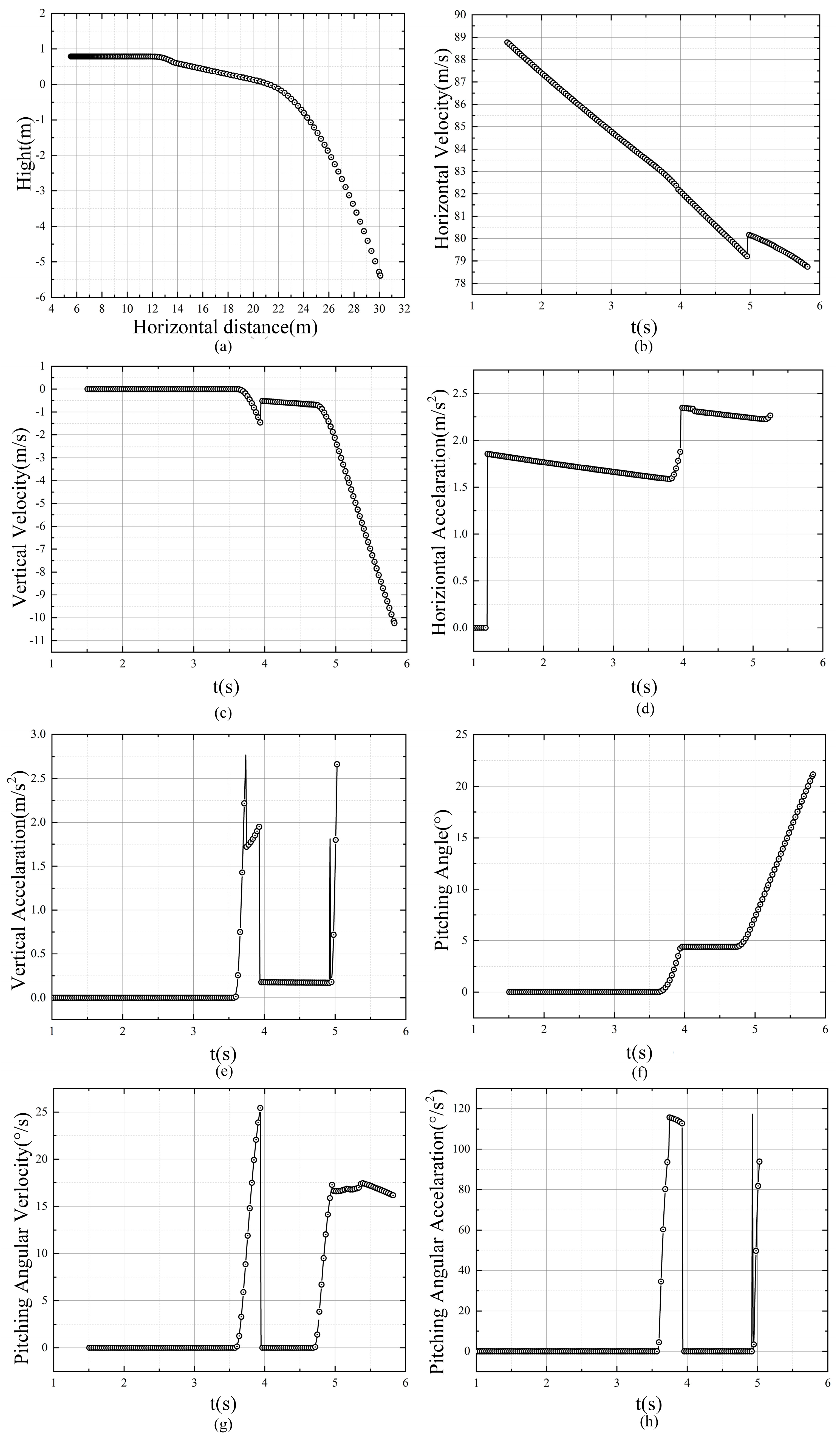
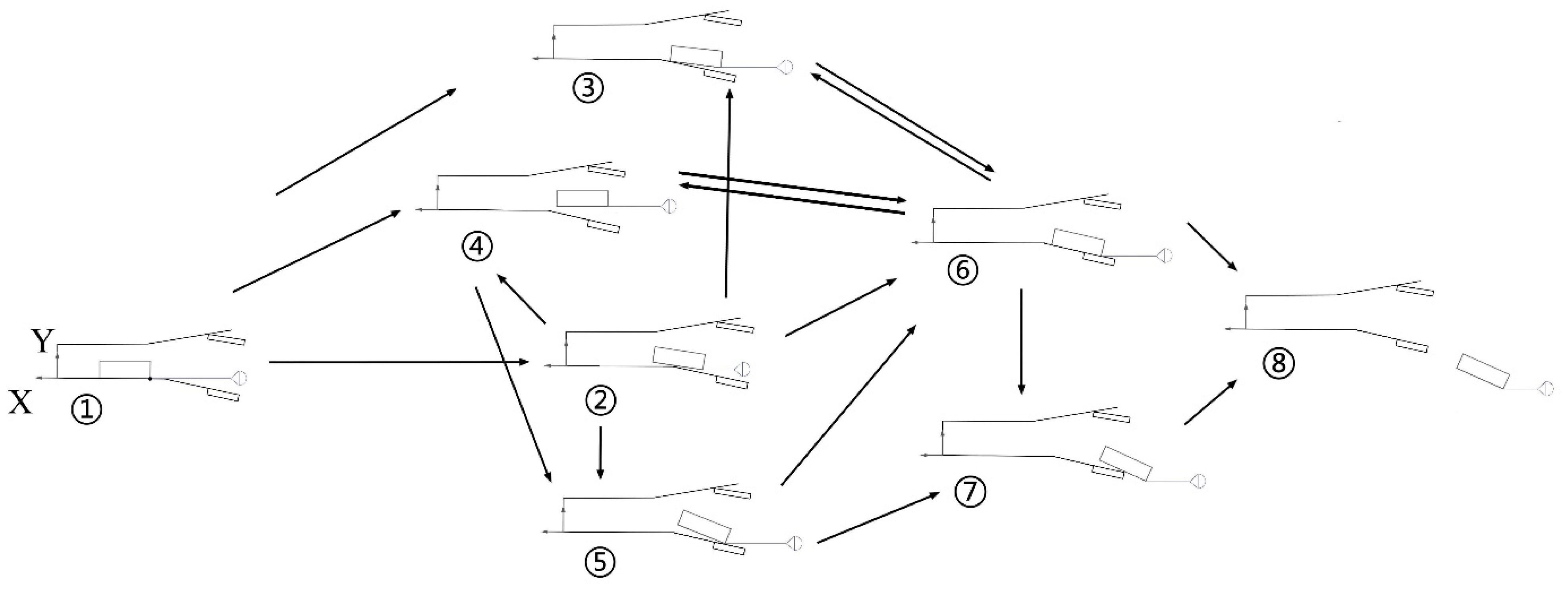
3.1.1. Results of Single Extra-Vehicular Process

A certain type of heavy-duty airdrop system is used to carry out the single extra-vehicular process analysis of the Kane equation dynamics model. The state parameters of the payload are shown in

Table 1. Payload state parameters.

Parameters	Value
Mass (kg)	7000
Profile (m3)	5.4 × 2.35 × 2.2
Airdrop Height (m)	600
Airdrop Velocity (km/h)	320
Installation Position (m)	8.34
Center of mass position factor	0.467
Flying Angle (°)	0

.

All the parachute parameters used for the process are shown in

Table 2. Parachute parameters.

Traction Parachute Line Parameters
Mass (kg)	2.83	Lenth (m)	3.47
Number of Roots	60	Number of Layers	1
Fracture strength (N)	4500	Modulus of elasticity (N)	15680
Pull-out resistance (N)	150
Traction parachute canopy parameters
Mass (kg)	3.47	Resistance Coefficient	0.777
Area (m2)	8	Pull-out resistance (N)	300
Traction parachute package parameters
Mass (kg)	2.68	Lenth (m)	0.5
Resistance characteristic (m2)	0.5
Main parachute package parameters
Mass (kg)	8.1	Resistance characteristic (m2)	0.14
Lenth (m)	1.36

.

The appropriate traction ratio is important to ensure the safety and attitude of the payload after departure. The traction ratio for the characterization of the process is defined as the ratio between the tractor pull F and the load gravity G, i.e., where K = F/G, $F=\rho v^2(CA)/2$. (CA) is the traction parachute drag characteristic, ρ is the air density, and v is the traction parachute airspeed. Therefore, the traction ratio is a dimensionless parameter that covers the airborne velocity, the drag characteristics of the parachute, and the mass of the payload.

The results are analyzed using a traction ratio of 0.2. The calculation is based on the initial condition, and the termination condition is 0.2 s after the tail section leaves the aircraft (the moment when the line is straightened), and the in-cabin motion characteristic curve of the payload is obtained. Figure 6a–h shows the trajectory of the payload center of mass, the horizontal velocity of the center of mass, the straight velocity of the center of mass, the horizontal acceleration of the center of mass, the vertical acceleration of the center of mass, the pitch angle, the pitch angle velocity, and the pitch angle acceleration, respectively, during the process of departure.

According to the analysis of the change curve of the motion status, the payload initially slides in the horizontal plane of the cargo bay, as described in the ground coordinate system, and the departure state is 1.507 s~5.824 s. The horizontal velocity gradually increases from 0 under the action of the traction parachute (only the horizontal velocity after the start of the exit state is intercepted in the figure), the vertical velocity remains unchanged, and the center of mass starts to rotate through the inflection point from 3.597 s, at which time the moment of gravity on the center of mass is greater than the pulling moment of the parachute line, after which the pitch angle and angular velocity increase rapidly. After 0.35 s, the rotation angle reaches the floor slope section tilt angle and the floor contact collision, causing the payload vertical direction velocity to change from −1.46 m/s to −0.51 m/s and the rotation angle velocity from 25.427°/s to 0. The acceleration and angular acceleration also change abruptly, then there is a slide along the cargo bay tilt section until the center of gravity passes through the floor slope edge (4.717 s), after which the pitch angle continues to rotate at an angle greater than the inclination angle of the floor tilt section until the tail is completely off the floor.

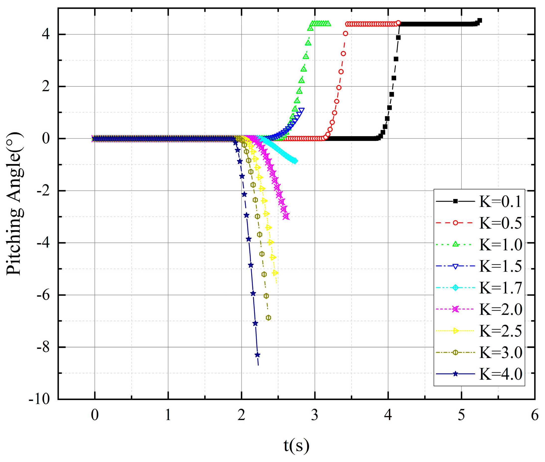
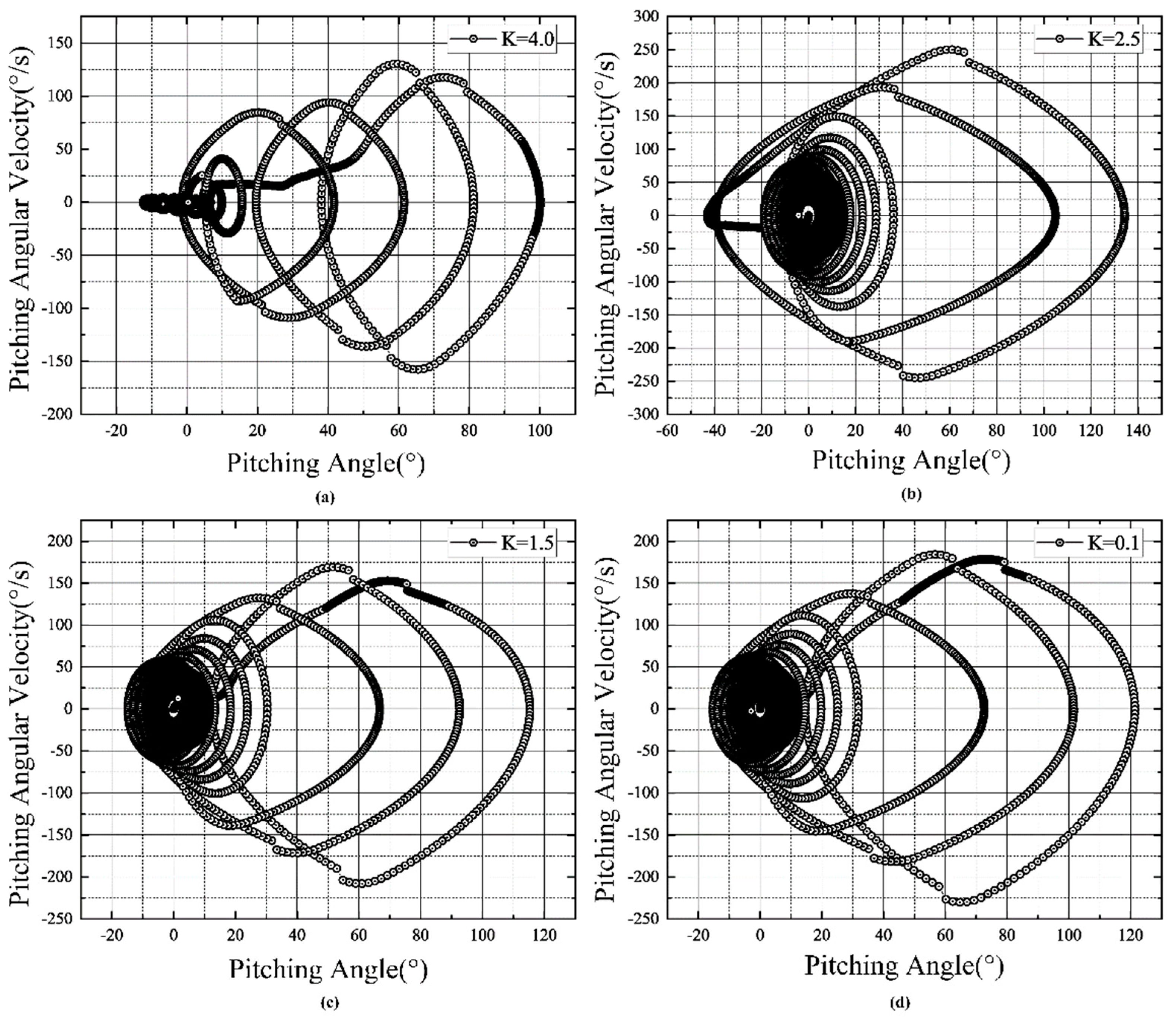
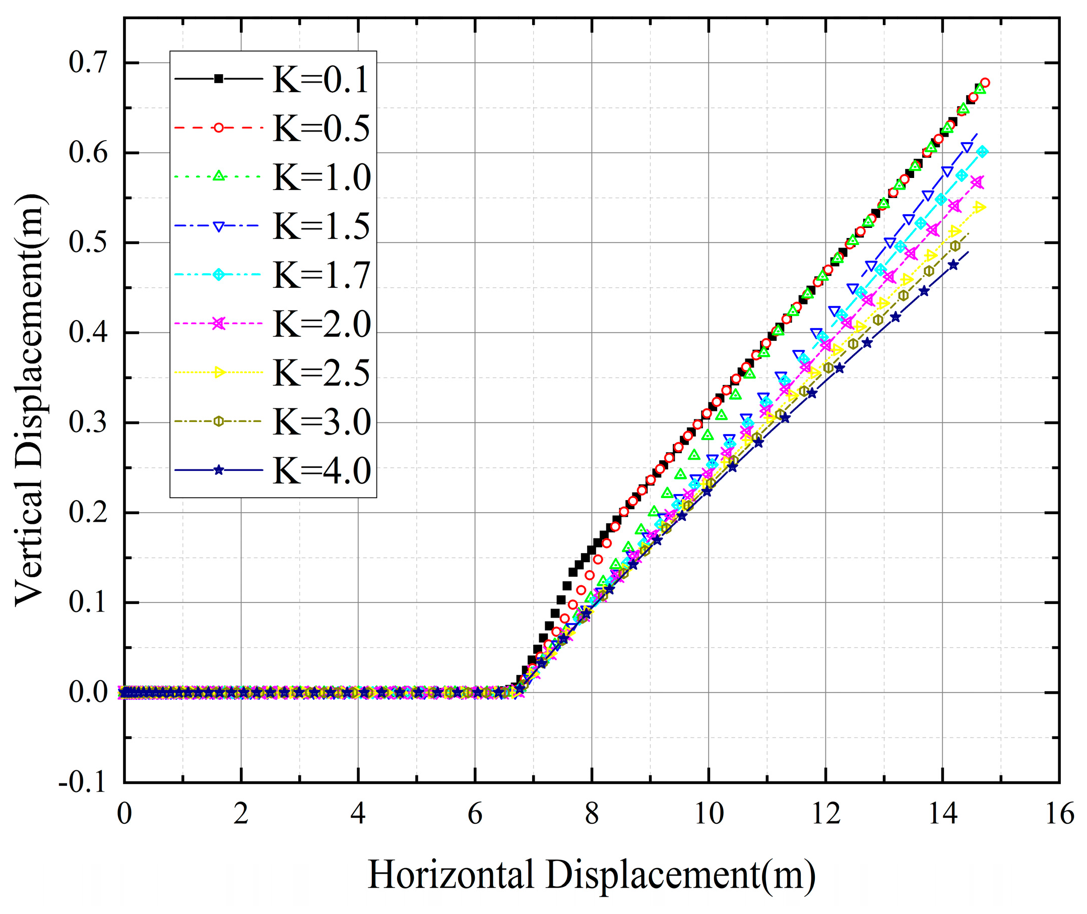
3.1.2. Results of Different Traction Ratios

Under the action of different traction ratios (0.2 ≤ K ≤ 4.0), the variation in the payload pitching angle with time during the extra-vehicular process is as shown in Figure 7. It can be seen from the figure that there are many types of payload attitude in the process with different traction ratios, and this process is greatly influenced by the traction ratio. When the traction ratio is small (K < 1.0), the payload slides along the tilted section of the floor after flipping forward through the inflection point (i.e., the front end sinks); when the traction ratio is large (K ≥ 1.0), the payload attitude changes are relatively complex and may appear in the middle to vacate or reverse when the traction moment at the bottom of the front end is large enough (i.e., the front end is pulled up). Regardless of the type of flip, the flip will end up in contact with the floor again and finally leave the aircraft from the tail section.

To further understand the effect of the traction ratio on the out-of-cabin motion, the phase plane trajectory of the payload pitching angle with the angular velocity for different traction ratios is given in Figure 8. The calculation keeps the airspeed of the aircraft constant during the airdrop, and the change in the traction ratio is achieved by changing the traction parachute drag characteristic size. The starting point (0,0) on the phase plane is also the final equilibrium point.

It can be seen from the figure that an increase in the traction ratio leads to a larger oscillation in both the pitch angle and the pitch angular velocity. At the same time, the phase plane oscillation caused by a larger traction ratio is different from that caused by a smaller traction ratio. For a larger traction, such as K = 0.4, the pitching angle oscillates further from the equilibrium point, thus causing the pitching angle to change more rapidly. Conversely, for smaller tractions, such as K = 0.1 or K = 1.5, the pitching angle oscillates nearer to the equilibrium point, thus causing the pitching angle to change in velocity more slowly.

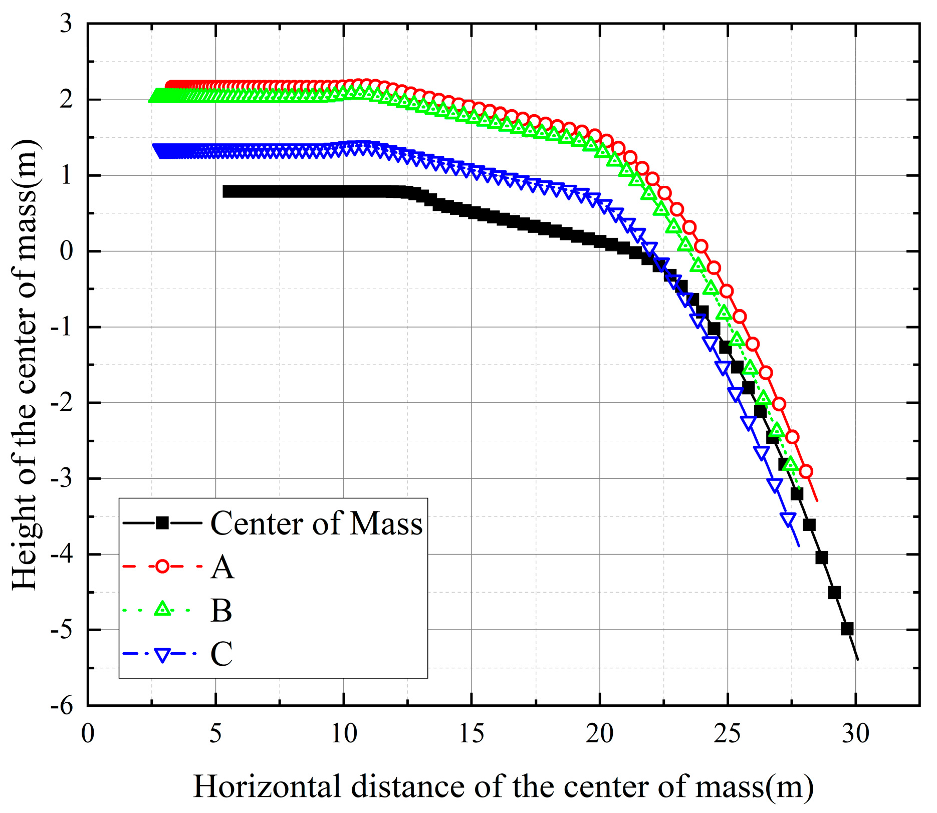
3.1.3. Off-Board Safety Analysis

The above results of the payload motion status changes during the process reveal that various flight conditions and system parameters pose a great challenge to the safe departure of the payload from the aircraft inside the cabin. Figure 9 shows the trajectories of the payload center of mass movement during the process under different traction ratios. In order to show the trajectory differences more visually, different scales are chosen for the X and Y direction axes. According to the analysis of the results under different traction ratios, as the traction ratio increases the speed of the payload through the inflection point also increases, and when the traction ratio increases to a certain degree, the payload will fly out directly without passing through the inclined section of the cargo hold or rotating counterclockwise. Therefore, although the increase in the traction ratio can reduce the payload extra-vehicular time, it will lead to a higher trajectory and reduce the safety space of the payload in the cabin, which is not conducive to off-board safety.

For further off-board safety analysis, define the danger point and calculate its most dangerous position and corresponding moment under a traction ratio of 0.2, as shown in

Table 3. Dangerous point coordinates.

Dangerous Point	Coordinates	Most Dangerous Position	Most Dangerous Time (s)
A	(4.3, 2.077, 0)	(10.8401, 2.1861, 0)	3.8370
B	(4.9, 1.938, 0)	(10.5749, 2.0737, 0)	3.8870
C	(4.746, 1.26, 0)	(10.6265, 1.3885, 0)	3.8770

.

In Figure 10, the center of gravity and the location of the danger point out of the cabin are shown schematically. This can be compared with the internal structural parameters of the cargo. By observing the coordinate changes in the figure and comparing the cabin structure coordinates, it can be concluded that the simulated payload extra-vehicular process is safe in this K = 0.2 condition.

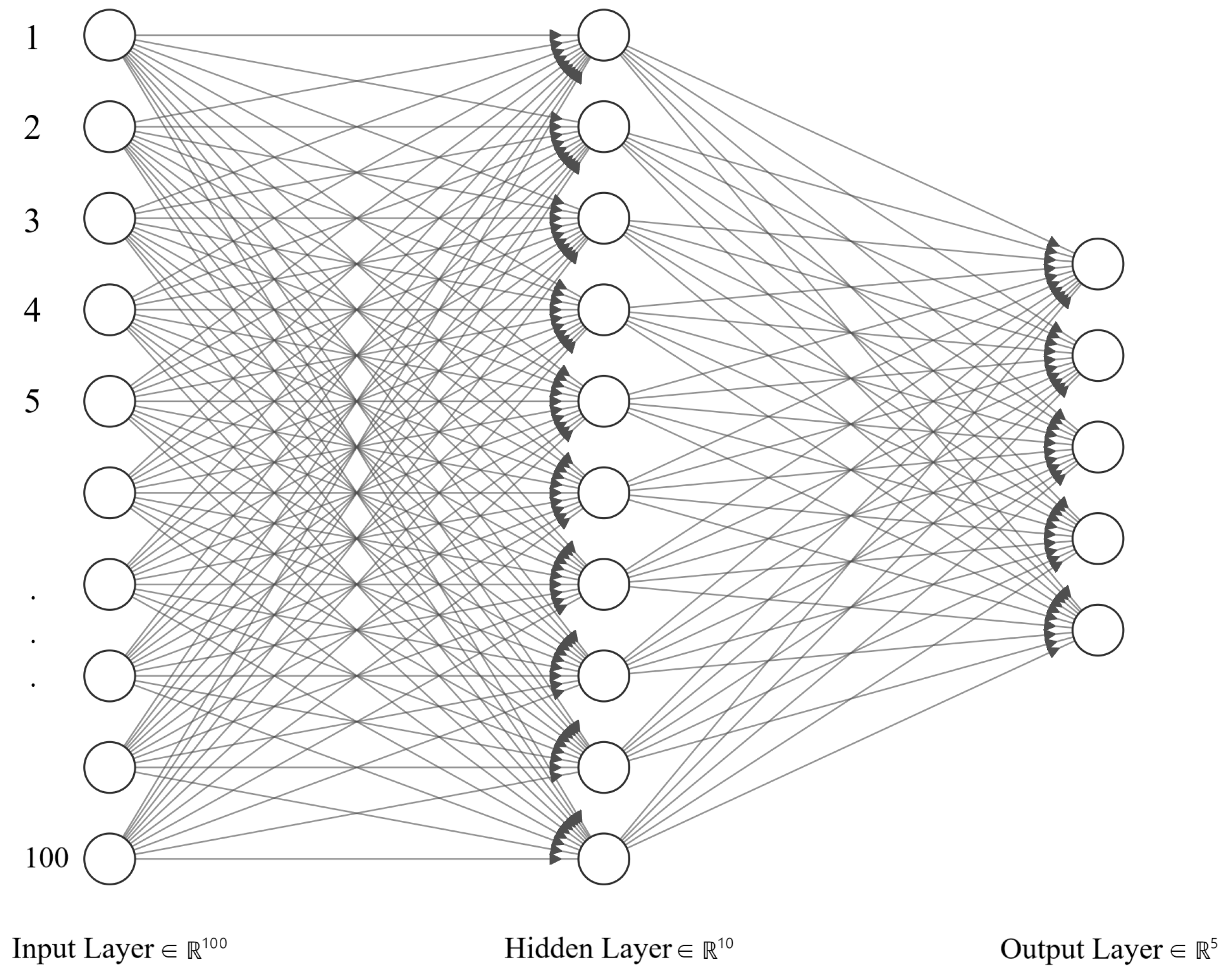
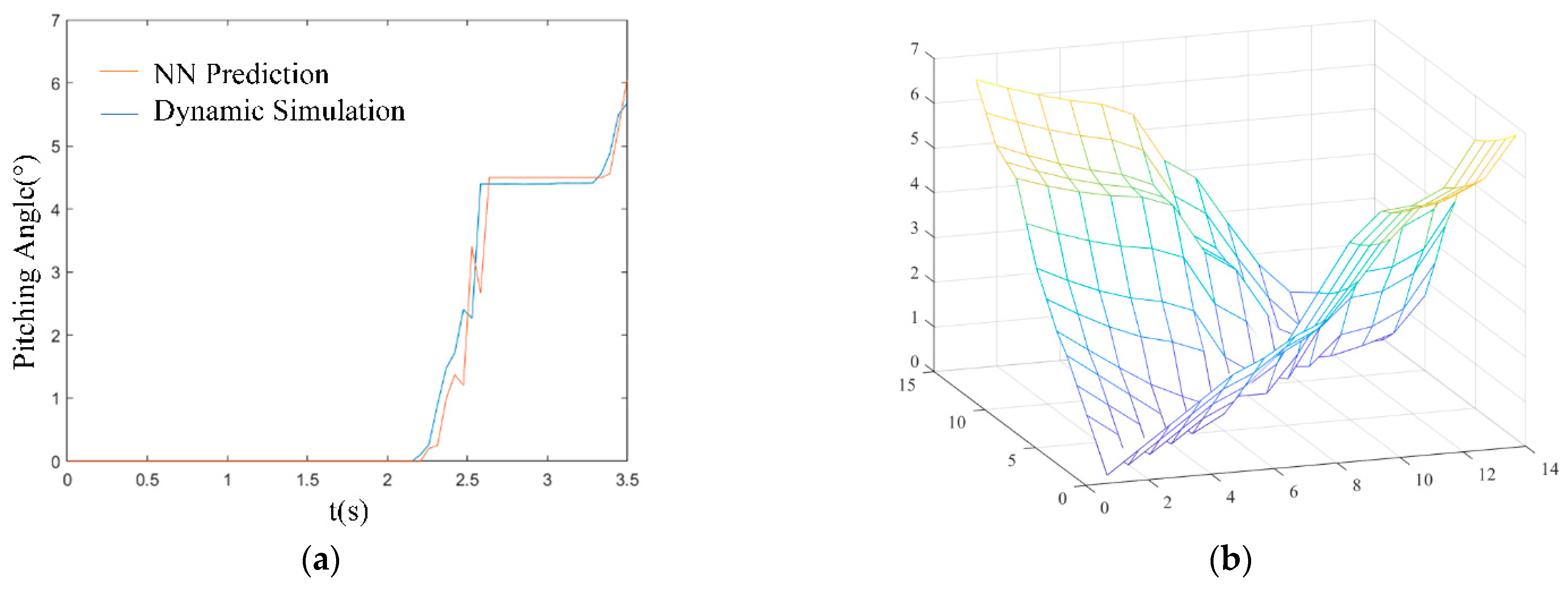
3.1.4. NN Status Recognition

In order to further clarify the relationship and connection between the payload and the ground contact status of the extra-vehicular process, the motion process conversion nodes and the corresponding payload cargo-hold ground position were identified by manual determination and neural network methods, respectively, to explore whether the NN had a high recognition rate of accuracy. The manually determined state relationship is shown in Figure 11.

The possible status of the payload was analyzed, then an attempt was made to introduce the NN approach for pattern recognition to the prediction of the samples provided by the dynamic simulation data. Firstly, the data source used for the NN in the paper was needed. The training data for the NN were pitching angle vectors. The simulation condition was the different traction ratios. The sample scale was 120. The input was the variation in the motion pitching angle over time, and the output was the different traction ratios. The traction ratio values were encoded as five-dimensional binary column vectors, with the first digit zero indicating that the traction ratio was greater than one and the first digit one indicating that the traction ratio was between zero and one.

As the target vector was a five-dimensional array, the output layer of the NN was also chosen to be five layers. The input layers and hidden layers were chosen from the characteristics of the dynamic simulation results array. The structure of the NN was selected and is shown in Figure 12. The activation function was ReLU. The percentages of the training data, validation data, and test data were 70%, 20%, and 10%, respectively. Multiple training sessions were conducted to select the appropriate epoch. Finally, the regression value, from the confusion matrix, was used to measure the prediction performance of the NN, and the results are shown in Figure 13.

The trained neural network is invoked to predict the pitching angle change corresponding to any given traction ratio. Taking the predicted state in Figure 14a as an example, the system goes through ①→④→②→③→⑥→⑦→⑧. The NN prediction compares perfectly to the simulation program results of the dynamics for continuous judgment and reproduction of the status. Figure 14b shows the Fletcher distance calculation process for two curves. A set of curves is randomly selected, and the discrete Fletcher distance, dF, is used to evaluate the magnitude of the error between the NN prediction and the true value, where the closer the dF value is to 0, the closer the two are; otherwise, the further away it is, the larger the error is. Finally, the dF for the predicted and true values = 0.5090, which is very small, is obtained for this simulation and is sufficient to meet the airdrop data accuracy requirements. The Fletcher distance is shown in Figure 14b. After a few iterations, as shown on the 3D surface, the minimum Fletcher distance dF is computed. The prediction of the NN matches well with the manually determined result.

In this way, by invoking the neural network, the status experienced by the payload under different airdrop conditions, such as the traction ratio conditions, can be obtained. The different status transitions are natural and conform well to the actual status changes, which greatly reduces the reliance on experimental data, and at the same time, random factors such as random wind fields are added, which also simulates well the uncertainty problem in the airdrop.

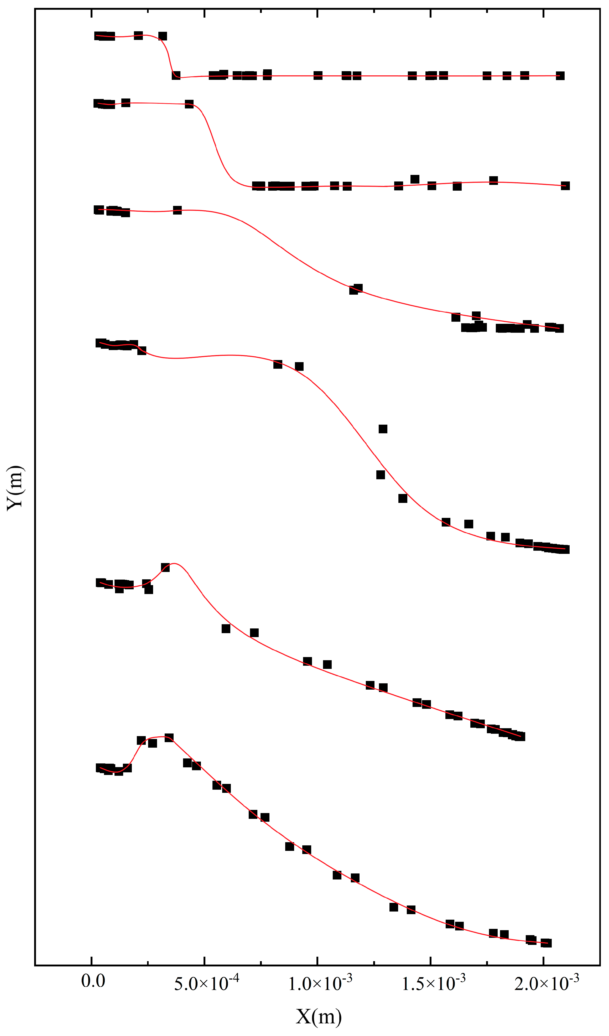
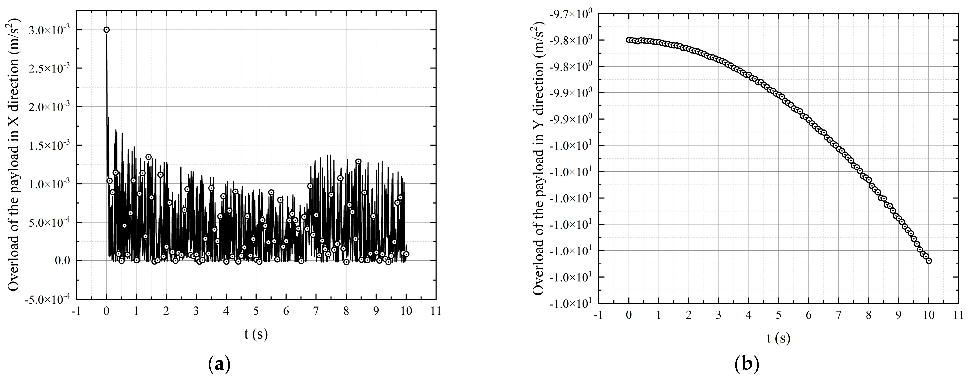
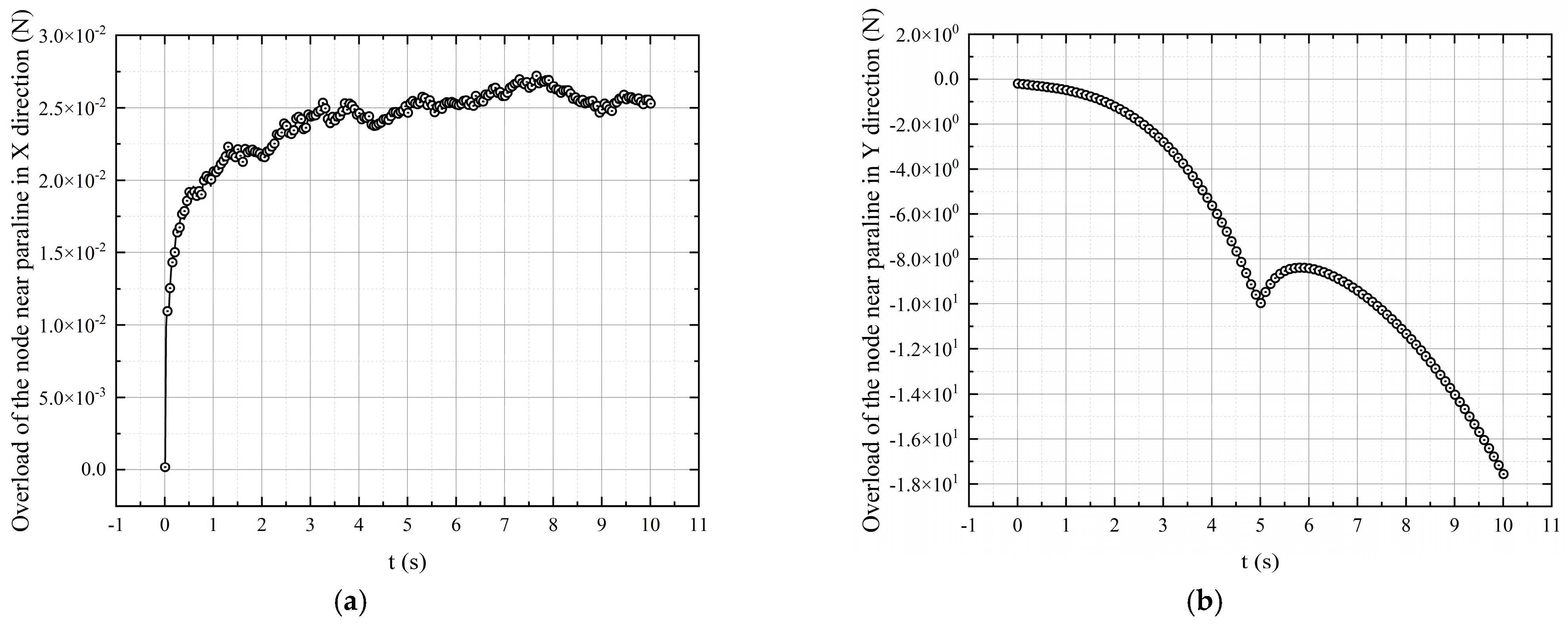
3.2. Results of Parachute Line Motion and Analysis

A mathematical–physical model of the parachute line based on the Kane equation outside the cabin was simulated to analyze the line sail phenomenon that occurs during the airdrop of missiles. The physical and geometric parameters of the components of the airdrop system are shown in

Table 4. Airdropped missile line sail phenomenon simulation parameters.

Parts	Parameters	Value	Unit
Missile	Mass	1088.435	kg
	Diameter	0.457	m
	Length	3.657	m
	Initial angle of attack	20	deg
	Initial velocity	1.28	Ma
Main Parachute	Diameter	14.020	m
	Mass	80	kg
Line	Length	15.239	m
	Diameter	0.006	m
	Mass	30	kg
Traction Parachute	Diameter	1.524	m
	Mass	8.0	kg

and are the same as the results from Purvis et al. [40]. The above weights were obtained under the condition that the fabric density was 600 kg/m³ and the parachute canopy was a hemispherical surface. The straightening process occurs at a flight speed of 1.28 Mach, and the missile has an angle of attack of 20° during the straightening process.

The calculated results are shown in Figure 15. In order to visualize the rope variation, the Y-value data of each state are ignored, and the denseness of the point-set of the plot lines is moderately reduced. The calculated results shown in the figure are compared with those from the literature, and it can be seen that the model can be better used to simulate the rope sail phenomenon that occurs in the test.

Figure 16 and Figure 17 give the overload variation curves in the x-direction and y-direction of the projectile in the above straightening overload and the tension variation curves of the nodes of the paracord adjacent to the projectile.

Observing the curves, it can be ascertained that the overload of the projectile in both directions, as well as the overload at the node of the parachute line, fluctuates to a large extent, mainly as a result of the propagation of the tension wave in the flexible parachute line. As the combined motion of the traction parachute under each force is basically along the horizontal direction, the x-direction acceleration acting on the projectile is an order of magnitude larger than that in the y-direction, excluding the gravity overload. In addition, the fluctuation of the overload in the x-direction is more drastic than that in the y-direction, which is due to the fact that the large amplitude of the stochastic wind model is in the x-direction, while the relatively small amplitude of the stochastic wind is distributed in the x- and y-directions. The random wind speed may be different from the actual situation. So, the feasibility of the Kane equation in simulating the complex dynamic behavior of the line straightening process is proved. Furthermore, the highly nonlinear nature of the flexible structure of the parachute line is responsible for the non-smoothness of the tension in the spring network reflected by the overload of the parachute line during the straightening process, i.e., the occurrence of violent fluctuations. The issue of curve fluctuations caused by the influence of other factors on the model can be left to subsequent studies.

4. Conclusions

In this study, the KE was used to model and simulate the dynamics of the out-of-cabin process and the extra-vehicular process. The out-of-cabin process analyzed the specific motion status and changes in the payload. The results of the motion were confirmed via the safety analysis. BPNNs were used for training the model to identify the status during multiple missions, whose efficiency was decided via the Fletcher distance (dF = 0.5090). In the extra-vehicular process, the parachute line form and overload were analyzed, and precise prediction results were obtained.

The Kane equation avoided the complex derivations required by Newtonian equations. Moreover, it had more universality and expandability. The BPNN made the identification of payload status repeatable and less reliant upon the experimental data. The spring network method made the line sail model even more expandable.

However, the continuation of the work in further studies, such as those on the prediction and analysis of performance in different and extreme working conditions of the airdrop process, is necessary. Furthermore, the reliance on the experimental data from the model in the paper could be weakened further by additional decoupling from the model. These remaining studies are still to be carried out in further work.

References

1. Bergeron, K.; Seidel, J.; Ghoreyshi, M. Numerical Study of Ram Air Airfoils and Upper Surface Bleed-Air Control. In Proceedings of the 32nd AIAA Applied Aerodynamics Conference, Atlanta, GA, USA, 16–20 June 2014. [Google Scholar] [CrossRef]
2. Goodrick, T. Theoretical study of the longitudinal stability of high-performance gliding airdrop systems. In Proceedings of the 5th Aerodynamic Deceleration Systems Conference, Albuquerque, NM, USA, 17–19 November 1975. [Google Scholar] [CrossRef]
3. Lingard, J.S. The Performance and DESIGN of Ram-Air Parachutes; T.R.-81-103; Royal Aircraft Establishment: Farnborough, UK, 1981. [Google Scholar]
4. Goodrick, T. Simulation studies of the flight dynamics of gliding parachute systems. In Proceedings of the 6th Aerodynamic Decelerator and Balloon Technology Conference, Houston, TX, USA, 5–7 March 1979. [Google Scholar] [CrossRef]
5. Goodrick, T. Comparison of simulation and experimental data for a gliding parachute in dynamic flight. In Proceedings of the 7th Aerodynamic Decelerator and Balloon Technology Conference, San Diego, CA, USA, 21–23 October 1981. [Google Scholar] [CrossRef]
6. Goodrick, T. Scale effects on performance of ram air wings. In Proceedings of the 8th Aerodynamic Decelerator and Balloon Technology Conference, Hyannis, MA, USA, 2–4 April 1984. [Google Scholar] [CrossRef]
7. Cockrell, D.; Haidar, N. Influence of the canopy-payload coupling on the dynamic stability in pitch of a parachute system. In Proceedings of the Aerospace Design Conference, Irvine, CA, USA, 16–19 February 1993. [Google Scholar] [CrossRef]
8. Machin, R.A.; Iacomini, C.S.; Cerimele, C.J.; Stein, J.M. Flight Testing the Parachute System for the Space Station Crew Return Vehicle. J. Aircr. 2001, 38, 786–799. [Google Scholar] [CrossRef]
9. Müller, S.; Wagner, O.; Sachs, G. A high-fidelity nonlinear multibody simulation model for parafoil systems. In Proceedings of the 17th AIAA Aerodynamic Decelerator Systems Technology Conference and Seminar, Monterey, CA, USA, 19–22 May 2003. [Google Scholar] [CrossRef]
10. Slegers, N.; Costello, M. Aspects of control for a parafoil and payload system. J. Guid. Control Dyn. 2003, 26, 898–905. [Google Scholar] [CrossRef]
11. Moog, R.D. Aerodynamic Line Bowing during Parachute Deployment. In Proceedings of the 5th Aerodynamic Deceleration Systems Conference, Albuquerque, NM, USA, 17–19 November 1975. [Google Scholar] [CrossRef]
12. Pillasch, D.W.; Shen, Y.C.; Valero, N. Parachute/submunition system coupled dynamics. In Proceedings of the 8th Aerodynamic Decelerator and Balloon Technology Conference, Hyannis, MA, USA, 2–4 April 1984. [Google Scholar] [CrossRef]
13. Fallon, E.J. Parachute dynamics and stability analysis of the Queen Match Recovery System. In Proceedings of the 11th Aerodynamic Decelerator Systems Technology Conference, San Diego, CA, USA, 9–11 April 1991. [Google Scholar]
14. Vishniak, A. Simulation of the payload-parachute-wing system flight dynamics. In Proceedings of the Aerospace Design Conference, Irvine, CA, USA, 16–19 February 1993. [Google Scholar] [CrossRef]
15. Wolf, D.F. Parachute opening shock. In Proceedings of the 15th Aerodynamic Decelerator Systems Technology Conference, Toulouse, France, 8–11 June 1999. [Google Scholar] [CrossRef]
16. Jia, T.; Amirouche, F. Optimum impact force in motion control of multibody systems subject to inequality contraints. Mech. Res. Commun. 1989, 16, 163–173. [Google Scholar] [CrossRef]
17. Ider, S.K. Modeling of control forces for kinematical constraints in multibody systems dynamics—A new approach. Comput. Struct. 1991, 38, 409–414. [Google Scholar] [CrossRef]
18. Saenger-Zetina, S.; Neiss, K.; Beck, R.; Abel, D. Optimal clutch control applied to a hybrid electric variable transmission with Kane equations. IFAC Proc. Vol. 2007, 40, 87–94. [Google Scholar] [CrossRef]
19. Quan, H.; Jia, Y.; Xu, S. A new computer-oriented approach with efficient variables for multibody dynamics with motion constraints. Acta Astronaut. 2012, 81, 380–389. [Google Scholar]
20. Salinic, S.; Boskovic, G.; Nikolic, M. Dynamic modelling of hydraulic excavator motion using Kane’s equations. Autom. Constr. 2014, 44, 56–62. [Google Scholar] [CrossRef]
21. Chowdhury, D. Kane model parameters and stochastic spin current. Solid State Commun. 2015, 222, 53–57. [Google Scholar] [CrossRef]
22. Liu, J.; Hearn, G.E.; Chen, X.; Jiang, Z.; Wu, G. Analysis of dynamic response of a restraining system for a powerless advancing ship based on the Kane method. Ocean Eng. 2016, 131, 114–134. [Google Scholar] [CrossRef]
23. Pal, R.S. Modelling of Helicopter Underslung Dynamics using Kane’s method. IFAC-Pap. Online 2020, 53, 536–542. [Google Scholar] [CrossRef]
24. Sharma, K.K.; Jee, G.; Rajeev, U.P.; Padmakumar, E.S. Modeling of the Helicopter Underslung Aircraft’s Lateral-Directional Dynamics. IFAC-Pap. Online 2022, 55, 174–179. [Google Scholar] [CrossRef]
25. Bagdonovich, B.; Desabrais, K.J.; Benney, R. Overview of the Precision Airdrop Improvement Four-Powers Long Term Technology Project. In Proceedings of the 17th AIAA Aerodynamic Decelerator Systems Technology Conference and Seminar, Monterey, CA, USA, 19–22 May 2003. [Google Scholar] [CrossRef]
26. Cuthbert, P.A. A software simulation of cargo drop tests. In Proceedings of the 17th AIAA Aerodynamic Decelerator Systems Technology Conference and Seminar, Monterey, CA, USA, 19–22 May 2003. [Google Scholar] [CrossRef]
27. Cuthbert, P.A.; Desabrais, J. Validation of a cargo airdrop software simulator. In Proceedings of the 17th AIAA Aerodynamic Decelerator Systems Technology Conference and Seminar, Monterey, CA, USA, 19–22 May 2003. [Google Scholar] [CrossRef]
28. Cuthbert, P.A.; Conley G, L. A Desktop Application to Simulate Cargo Drop Tests. In Proceedings of the 18th AIAA Aerodynamic Decelerator Systems Technology Conference and Seminar, Munich, Germany, 23–26 May 2005. [Google Scholar] [CrossRef]
29. Taylor, A.P.; Murphy, E. The DCLDYN Parachute Inflation and Trajectory Analysis Tool—An Overview. In Proceedings of the 18th AIAA Aerodynamic Decelerator Systems Technology Conference and Seminar, Munich, Germany, 23–26 May 2005. [Google Scholar] [CrossRef]
30. Ke, P.; Yang, C.X.; Yang, X.S. Extraction Phase Simulation of Cargo Airdrop System. Chin. J. Aeronaut. 2006, 19, 315–321. [Google Scholar] [CrossRef]
31. Liu, Y.H.; Wang, H.L.; Fan, J.X.; Wu, J.F.; Wu, T.C. Control-oriented UAV highly feasible trajectory planning: A deep learning method. Aerosp. Sci. Technol. 2020, 110, 106435. [Google Scholar] [CrossRef]
32. Pereira, G.; Oliveira, M.; Ebecken, N. Genetic Optimization of Artificial Neural Networks to Forecast Virioplankton Abundance from Cytometric Data. J. Intell. Learn. Syst. Appl. 2013, 5, 57–66. [Google Scholar] [CrossRef]
33. Hu, L.; Zhang, J.; Xiang, Y.; Wang, W. Neural Networks-Based Aerodynamic Data Modeling: A Comprehensive Review. IEEE Access 2020, 8, 90805–90823. [Google Scholar] [CrossRef]
34. Li, K.; Kou, J.Q.; Zhang, W.W. Deep neural network for unsteady aerodynamic and aeroelastic modeling across multiple Mach numbers. Nonlinear Dyn. 2019, 96, 2157–2177. [Google Scholar] [CrossRef]
35. Giorgi, M.G.D.; Quarta, M. Hybrid MultiGene Genetic Programming—Artificial neural networks approach for dynamic performance prediction of an aeroengine. Aerosp. Sci. Technol. 2020, 103, 105902. [Google Scholar] [CrossRef]
36. Farabet, C.; Coupri, C.; Najman, L. Learning hierarchical features for scene labeling. IEEE Trans. Pattern Anal. Mach. Intell. 2013, 35, 1915–1929. [Google Scholar] [CrossRef] [PubMed]
37. Wang, L.R. Parachute Theory and Application; Aerospace Press: Beijing, China, 1997. (In Chinese) [Google Scholar]
38. Moog, R.D.; Bacchus, D.L.; Utreja, L.R. Performance evaluation of Space Shuttle SRB parachutes from air drop and scaled model wind tunnel tests <149>Solid Rocket Booster recovery system. In Proceedings of the 6th Aerodynamic Decelerator and Balloon Technology Conference, Houston, TX, USA, 5–7 March 1979. [Google Scholar] [CrossRef]
39. Purvis, J.W. Prediction of line sail during lines-first deployment. In Proceedings of the 21st Aerospace Sciences Meeting, Reno, NV, USA, 10–13 January 1983. [Google Scholar] [CrossRef]
40. Purvi, J.W. Improved prediction of parachute line sail during lines-first deployment. In Proceedings of the 8th Aerodynamic Decelerator and Balloon Technology Conference, Hyannis, MA, USA, 2–4 April 1984. [Google Scholar] [CrossRef]
41. Johnson, D.W. Testing of a new recovery parachute system for the F111 aircraft crew escape module: An update. In Proceedings of the 10th Aerodynamic Decelerator Conference, Cocoa Beach, FL, USA, 18–20 April 1989. [Google Scholar] [CrossRef]
42. Peterson, C.W. High Performance Parachutes. Sci. Am. 1990, 262, 108–116. [Google Scholar] [CrossRef]
43. Maydew, R.C.; Peterson, C.W.; Orlik-Rueckemann, K.J. Design and Testing of High-Performance Parachutes; NATO Advisory Group for Aerospace Research and Development (AGARD): Neuilly-Sur-Seine, France, 1991. [Google Scholar]
44. Wang, Y.; Yang, C.; Yang, H. Neural network-based simulation and prediction of precise airdrop trajectory planning. Aerosp. Sci. Technol. 2022, 1, 120. [Google Scholar] [CrossRef]
45. Adelfang, S.I.; Smith, O.E. Gust models for launch vehicle ascent. In Proceedings of the 36th AIAA Aerospace Sciences Meeting and Exhibit, Reno, NV, USA, 12–15 January 1998. [Google Scholar] [CrossRef]
46. Wang, H. Dynamic Modeling and Simulation of Whipping Phenomenon for Large Parachute. AIAA J. 2018, 56, 1–11. [Google Scholar] [CrossRef]
47. Zhang, Q.B.; Cheng, W.K.; Peng, Y.; Qin, Z.Z. A Multi-Rigid-body Model of Parachute Deployment. Chin. Space Sci. Technol. 2003, 23, 45–50. (In Chinese) [Google Scholar]
48. Huston, R.L. On the equivalence of Kane’s equations and Gibbs’ Equations for multibody dynamics formulations. Mech. Res. Commun. 1987, 14, 123–131. [Google Scholar] [CrossRef]
Figure 1. Line sail phenomenon.
Aerospace 10 00905 g001
Figure 2. Physical model of the system and multibody dynamics connection diagram.
Aerospace 10 00905 g002
Figure 3. Two types of status where the payload is in contact with the floor of the cabin: (a) line to point, and (b) line to surface.
Aerospace 10 00905 g003
Figure 4. The parachute straightening process.
Aerospace 10 00905 g004
Figure 5. Spring network model and node mass distribution for the straightening process of the parachute payload system.
Aerospace 10 00905 g005
Figure 6. Payload motion status in the extra−vehicular process (K = 0.2): (a) trajectory; (b) horizontal velocity; (c) vertical velocity; (d) horizontal acceleration; (e) vertical acceleration; (f) pitching angle; (g) pitching angular velocity; and (h) pitching angular acceleration.
Aerospace 10 00905 g006
Figure 7. Variation in payload pitching angle during the extra−vehicular process under different traction ratios.
Aerospace 10 00905 g007
Figure 8. Phase plane trajectory between the pitching angle and the pitching angular velocity for different traction ratio loads.
Aerospace 10 00905 g008
Figure 9. Trajectory of the center of mass with different traction ratios.
Aerospace 10 00905 g009
Figure 10. Trajectory of center of gravity and position of danger point (K = 0.2).
Aerospace 10 00905 g010
Figure 11. Relationship between the payload and the ground contact status in the cabin.
Aerospace 10 00905 g011
Figure 12. Neural network structure.
Aerospace 10 00905 g012
Figure 13. NN prediction confusion matrix results.
Aerospace 10 00905 g013
Figure 14. Comparison of trained NN predictions with true values and Fletcher distance calculation process: (a) one single prediction; and (b) the discrete Fletcher distance in the single prediction.
Aerospace 10 00905 g014
Figure 15. Simulation results of different moments corresponding to the parachute line form.
Aerospace 10 00905 g015
Figure 16. The bullet body overload curve. (a) overload of the payload in X direction (b) overload of the payload in Y direction.
Aerospace 10 00905 g016
Figure 17. Overload variation curve at the node of the parachute line near the bullet body. (a) overload of the node near paraline in X direction (b) overload of the node near paraline in Y direction.
Aerospace 10 00905 g017