

The Aerodynamic Performance of a Novel Overlapping Octocopter Considering Horizontal Wind


Abstract
:1. Introduction
2. Analysis of the Theoretical Model
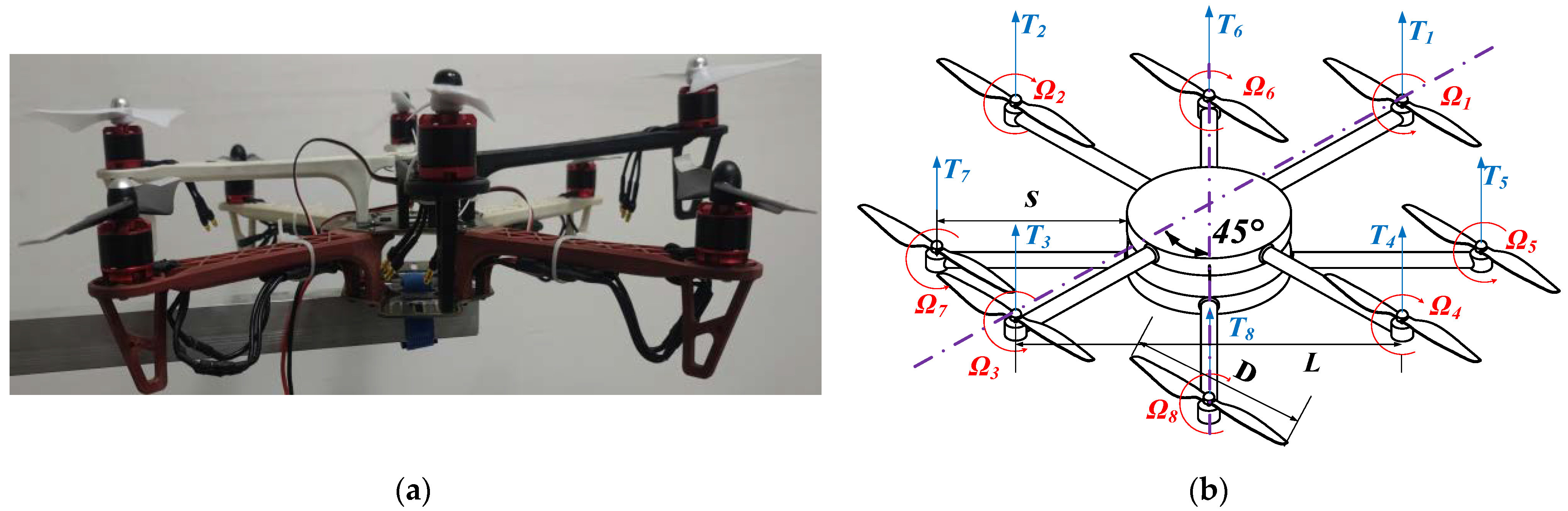
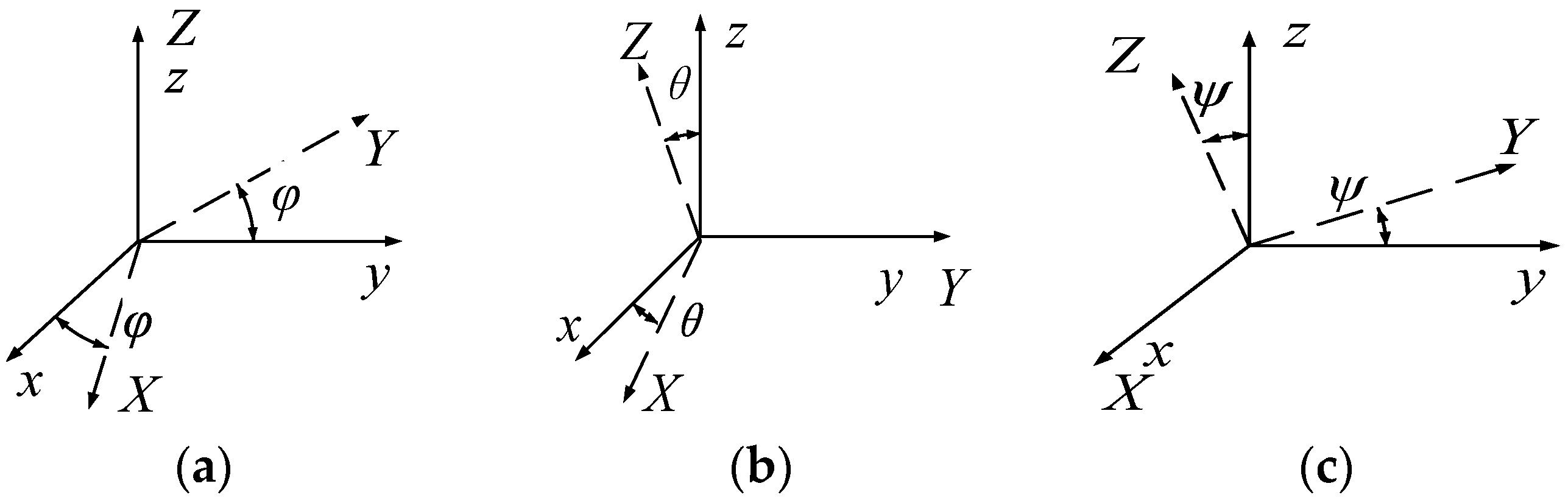
2.1. Model Dynamics
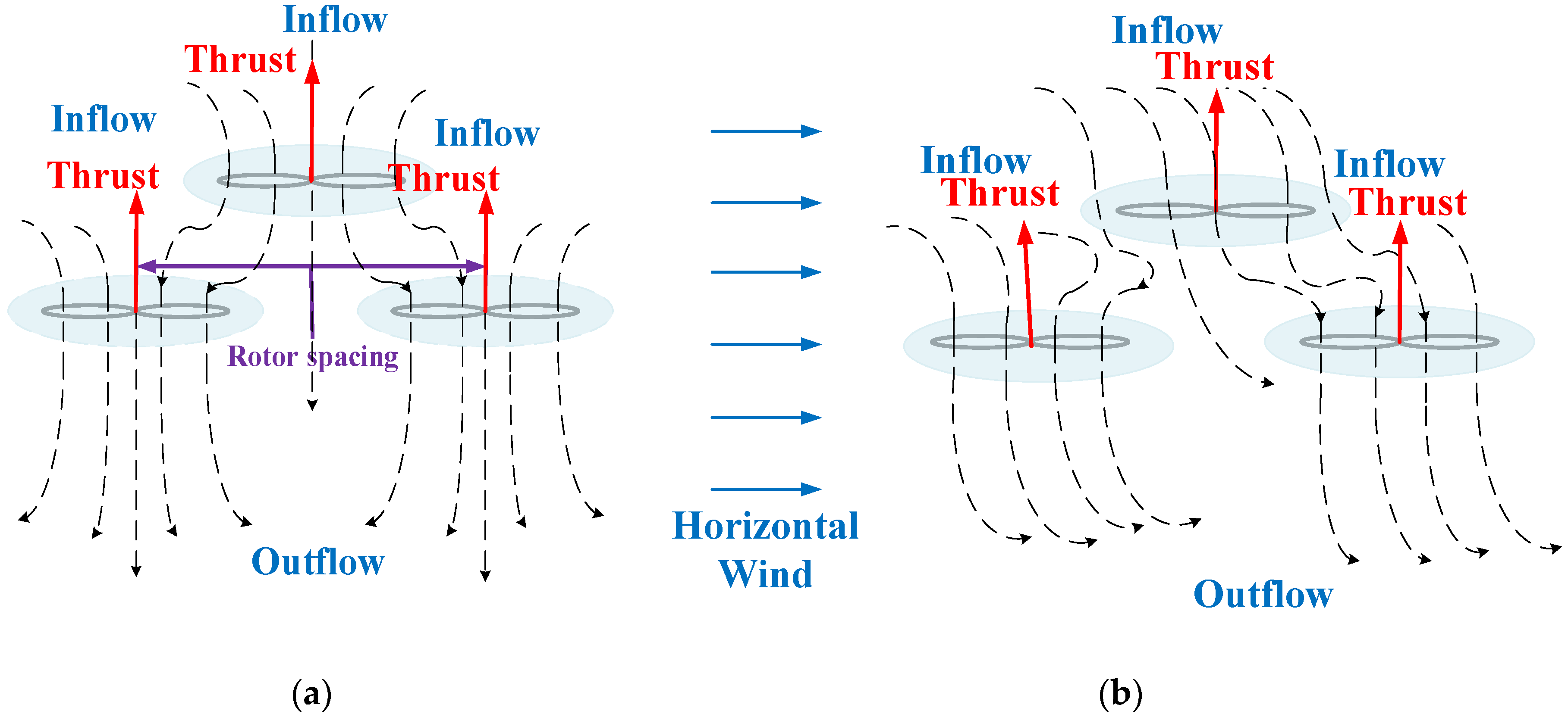
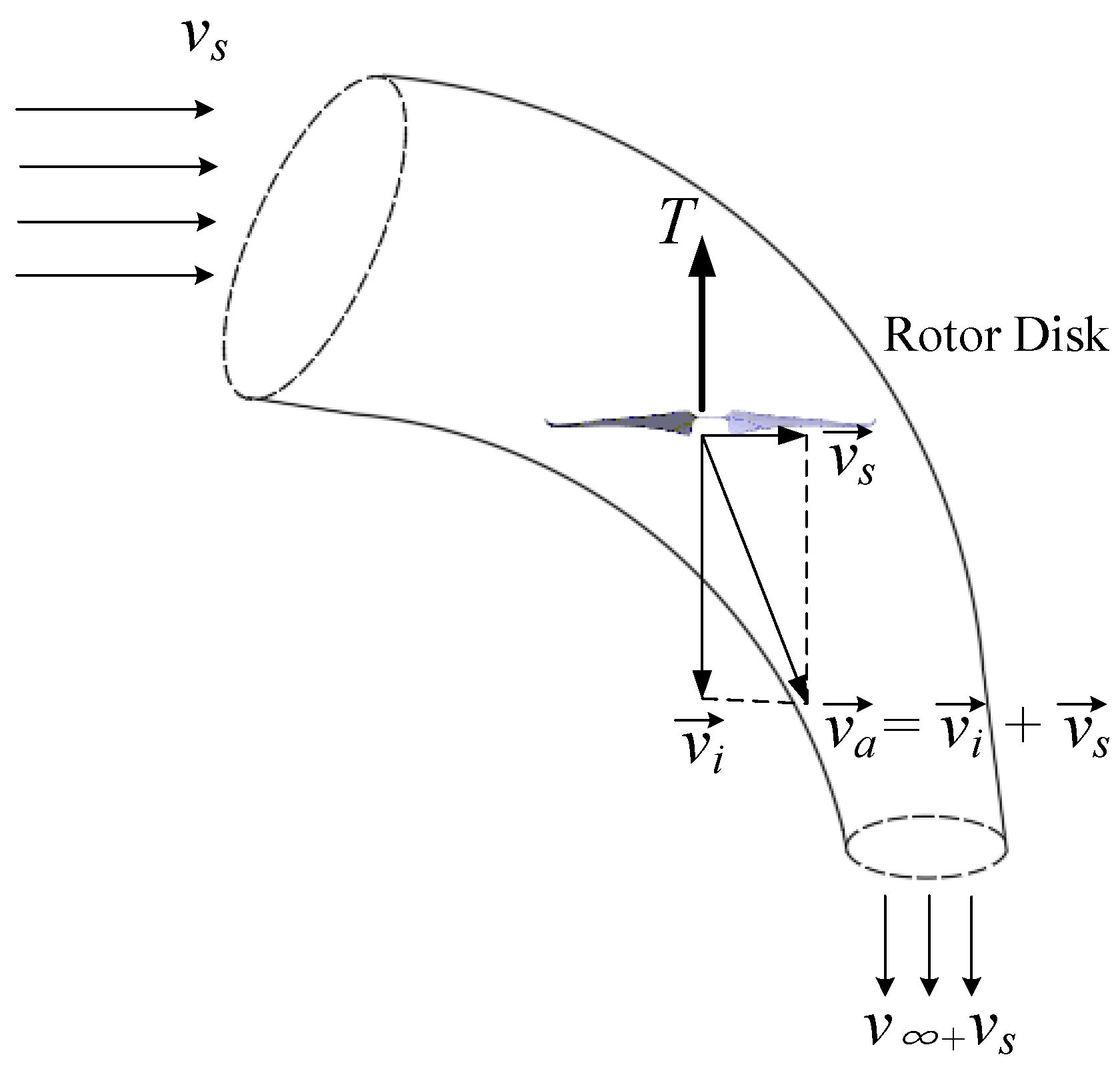
2.2. Aerodynamic Model
3. Simulations
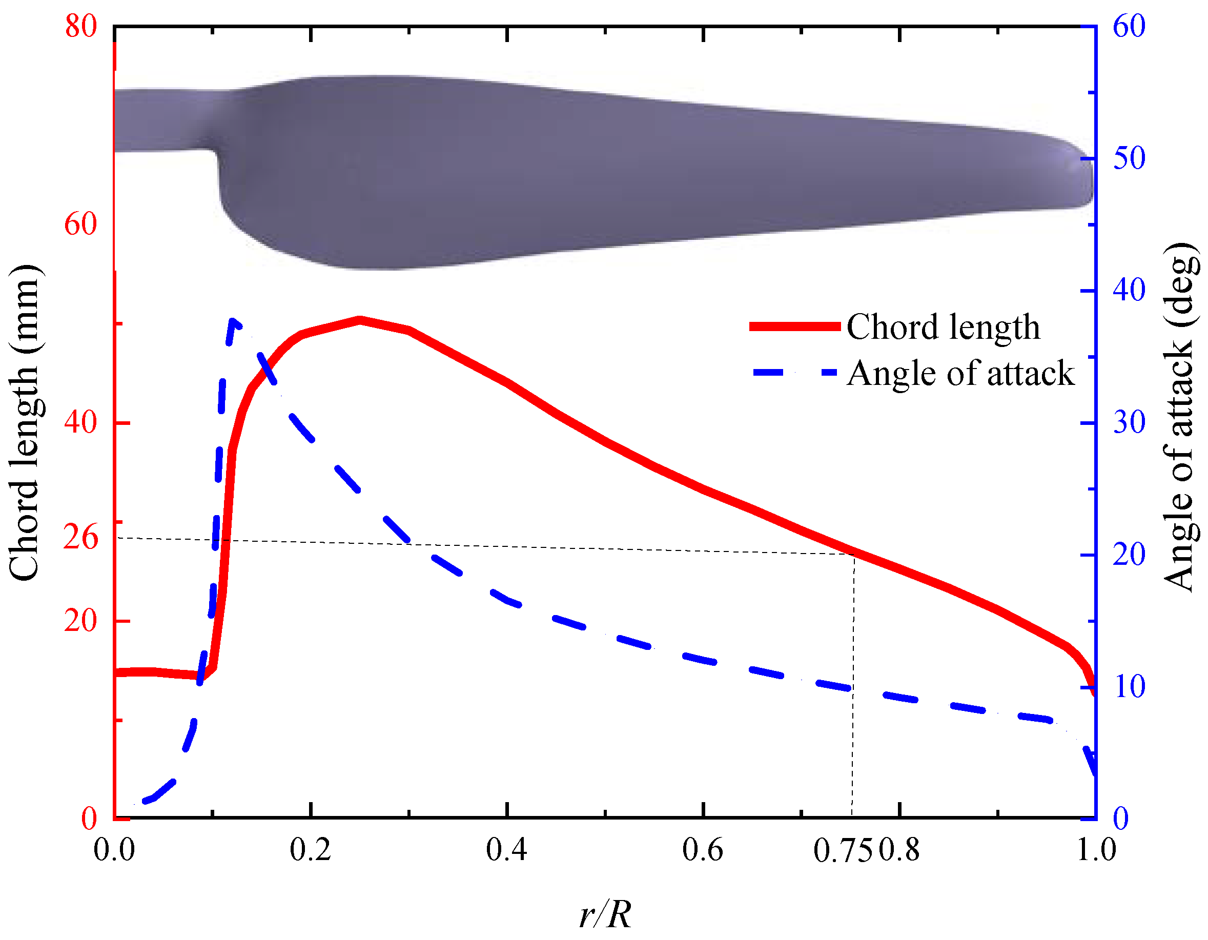
3.1. Geometry
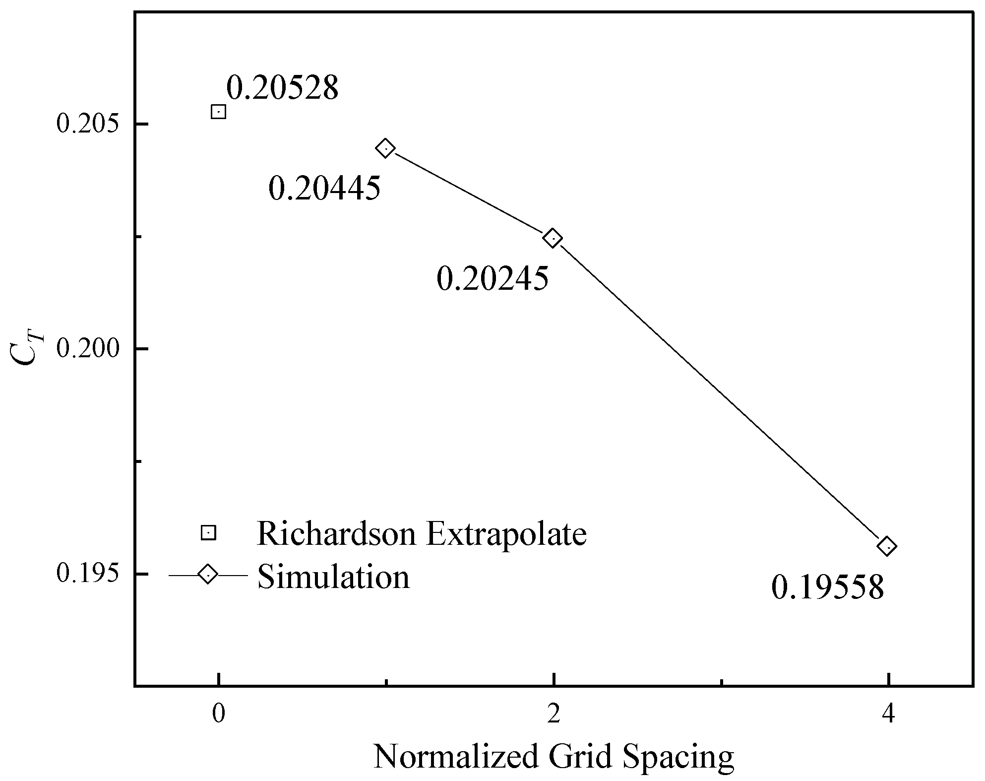
3.2. Mesh Domain
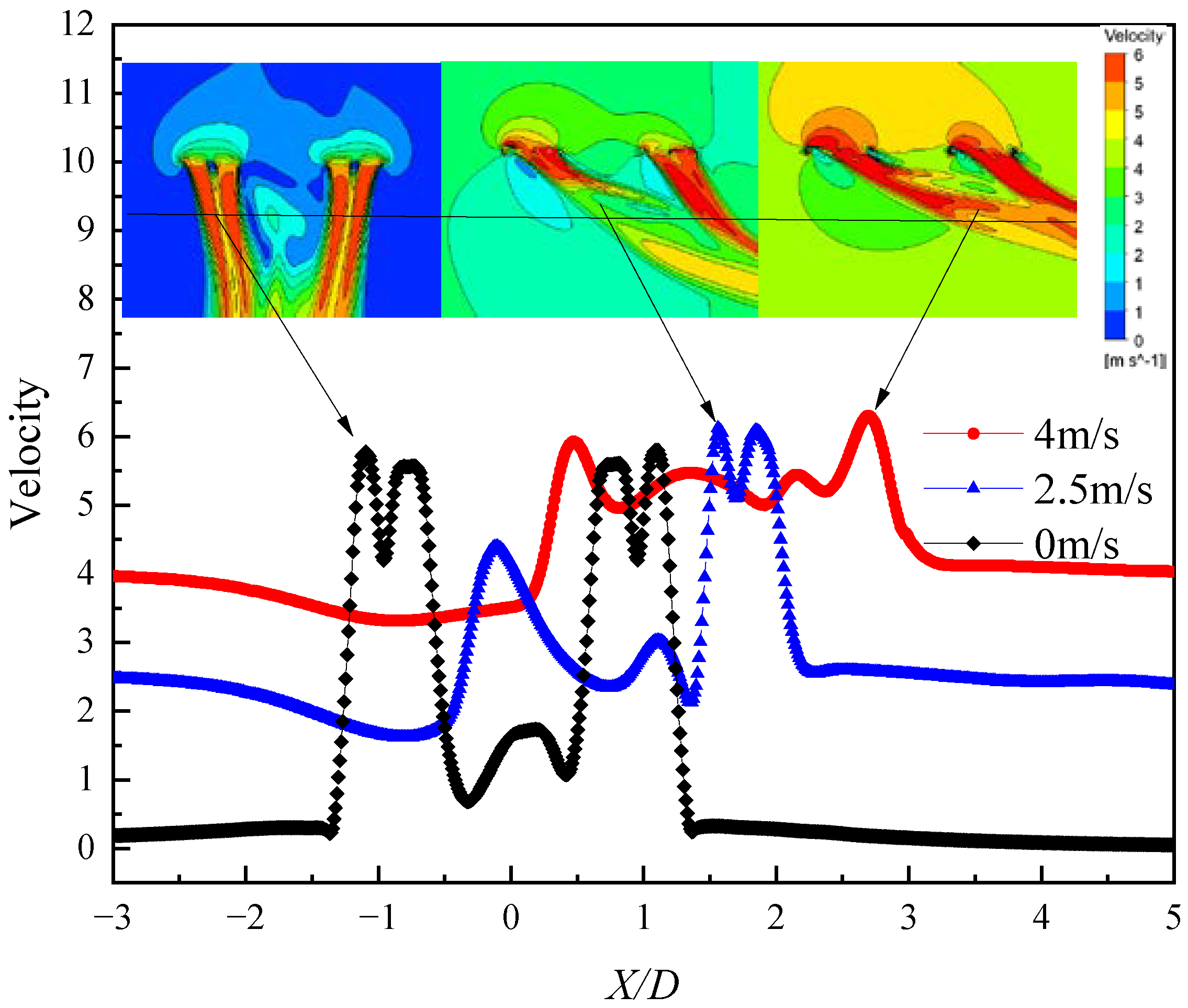
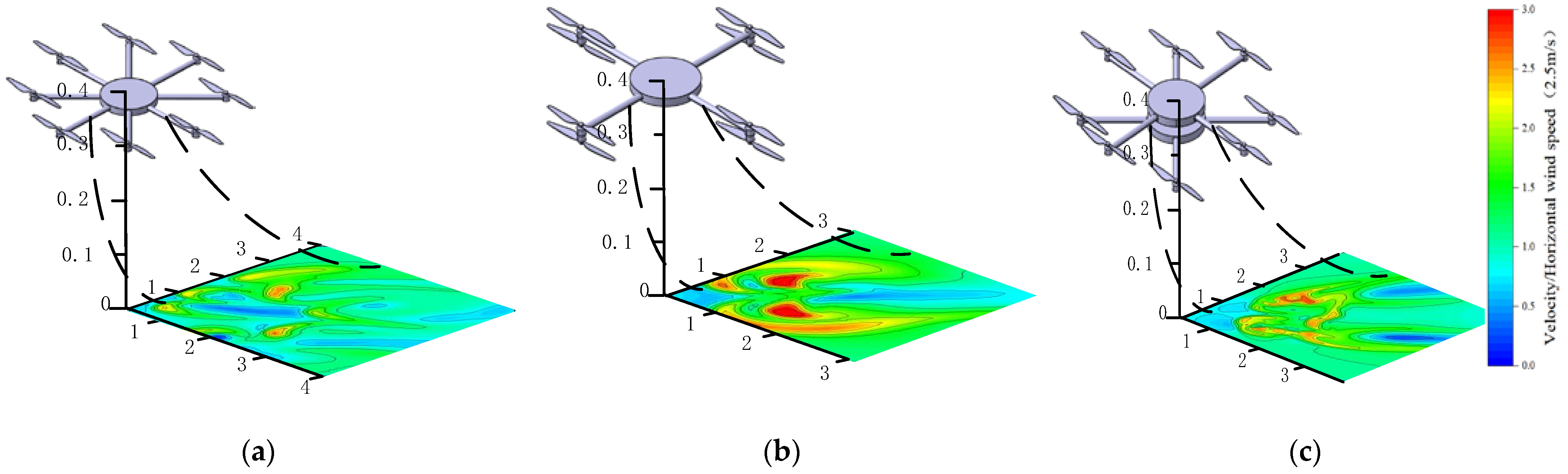
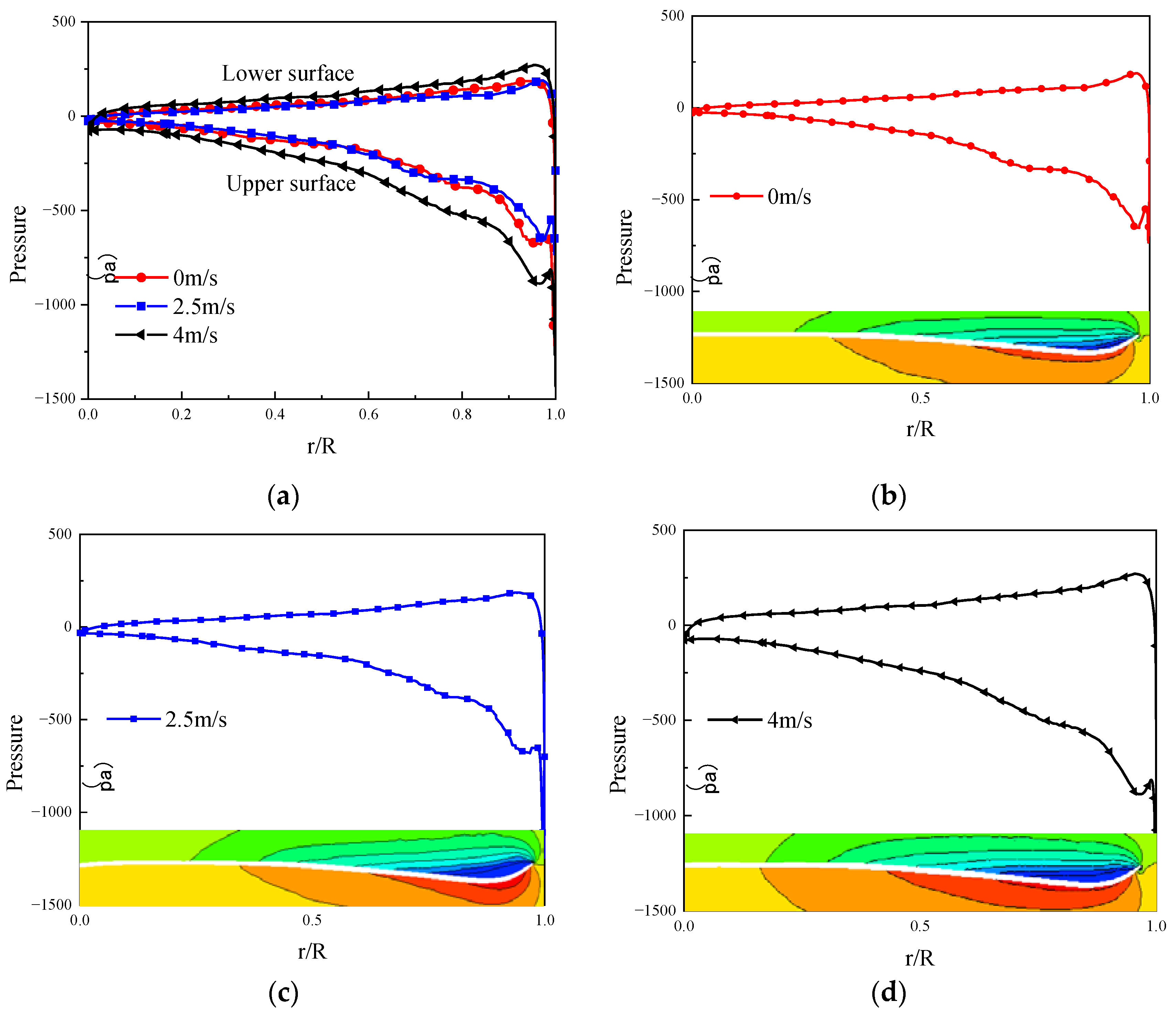
3.3. Results
4. Wind Tunnel Tests
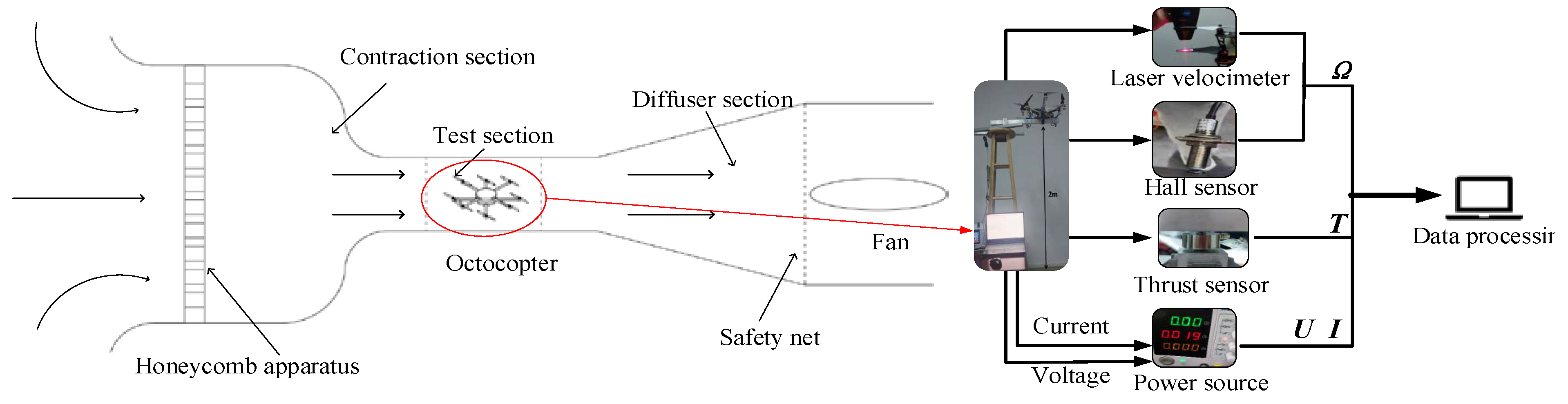
4.1. Facility and Experimental Setup
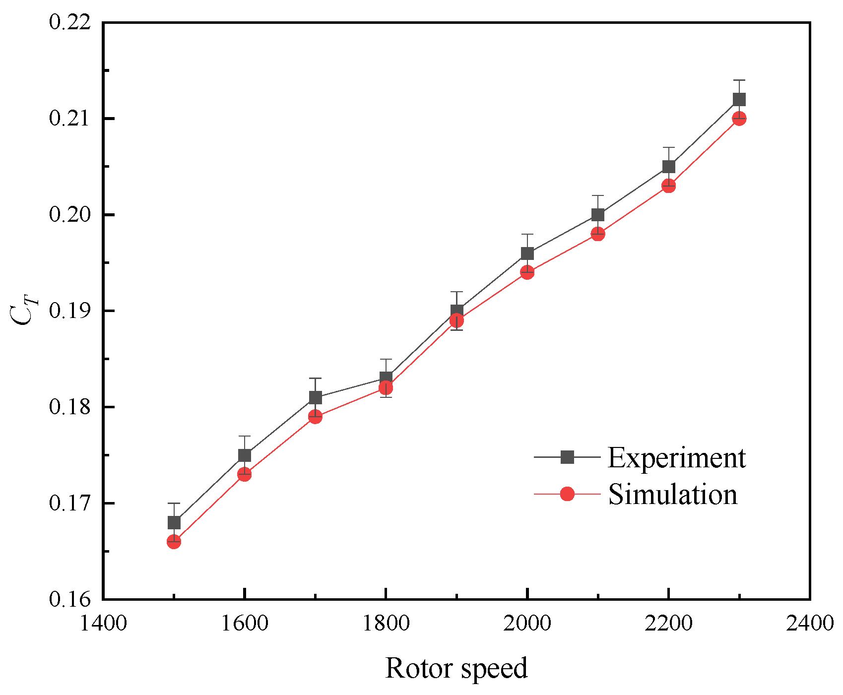
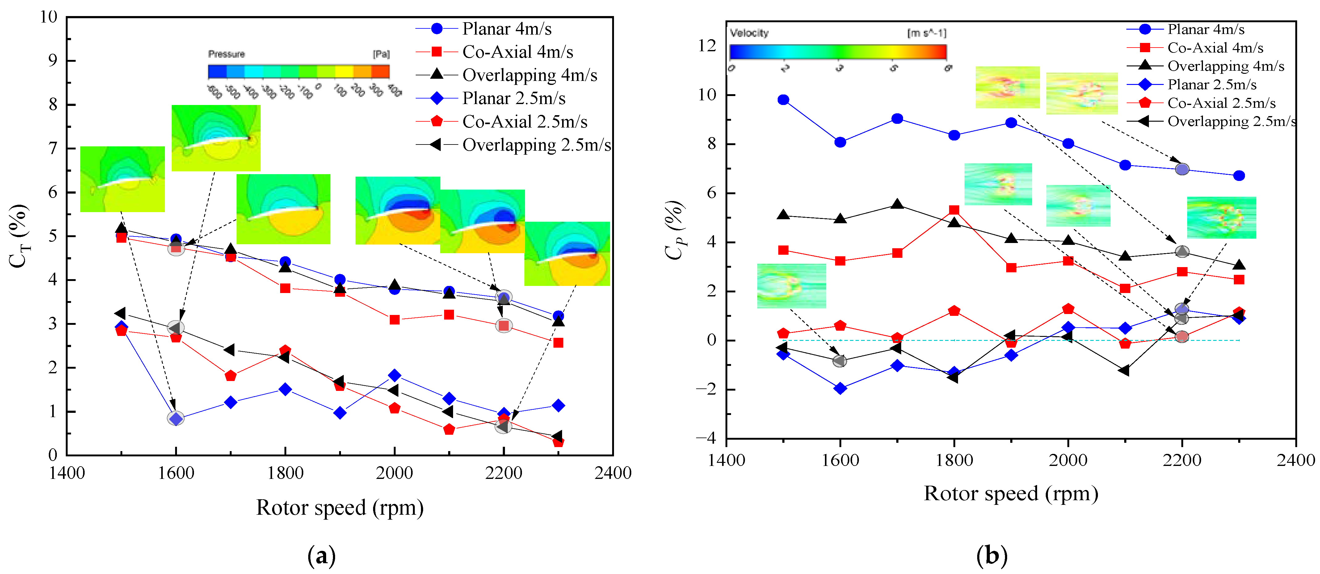
4.2. Results
5. Conclusions
Author Contributions
Funding
Data Availability Statement
Acknowledgments
Conflicts of Interest
References
- Nawaz, H.; Ali, H.M.; Massan, S. Applications of unmanned aerial vehicles: A review. Tecnol. Glosas InnovaciÓN Apl. Pyme. Spec 2019, 2019, 85–105. [Google Scholar] [CrossRef]
- AL-Dosari, K.; Hunaiti, Z.; Balachandran, W. Systematic Review on Civilian Drones in Safety and Security Applications. Drones 2023, 7, 210. [Google Scholar] [CrossRef]
- Liu, Z.; Li, J. Application of Unmanned Aerial Vehicles in Precision Agriculture. Agriculture 2023, 13, 1375. [Google Scholar] [CrossRef]
- Jalayer, M.; O’Connell, M.; Zhou, H.; Szary, P.; Das, S. Application of Unmanned Aerial Vehicles to Inspect and Inventory Interchange Assets to Mitigate Wrong-Way Entries. ITE J. 2019, 36, 42. [Google Scholar]
- Aboulafia, R. Military rotorcraft: Strongest aero market. Aerosp. Am. 2011, 49, 8. [Google Scholar]
- Basset, P.M.; Vu, B.D.; Beaumier, P.; Reboul, G.; Ortun, B. Models and Methods at ONERA for the Presizing of eVTOL Hybrid Aircraft Including Analysis of Failure Scenarios. In Proceedings of the AHS International 74th Annual Forum & Technology Display, Phoenix, AZ, USA, 14–17 May 2018. [Google Scholar]
- Wei, P.; Lin, X.; Kong, Z. System identification of wind effects on multirotor aircraft. Int. J. Intell. Robot. Appl. 2021, 6, 1. [Google Scholar] [CrossRef]
- González-Rocha, J.; De Wekker, S.F.; Ross, S.D.; Woolsey, C.A. Wind Profiling in the Lower Atmosphere from Wind-Induced Perturbations to Multirotor UAS. Sensors 2020, 20, 1341. [Google Scholar] [CrossRef]
- Tong, C.; Liu, Z.; Dang, Q.; Wang, J.; Cheng, Y. Online environmentally adaptive trajectory plan-ning for rotorcraft unmanned aerial vehicles. Aircr. Eng. Aerosp. Technol. 2023, 95, 2. [Google Scholar]
- Sisson, W.; Karve, P.; Mahadevan, S. Digital twin for component health- and stress-aware rotorcraft flight control. Struct. Multidiscip. Optim. 2022, 65, 11. [Google Scholar] [CrossRef]
- Park, H.S.; Linton, D.; Thornber, B. Rotorcraft fuselage and ship airwakes simulations using an immersed boundary method. Int. J. Heat Fluid Flow 2022, 9, 3. [Google Scholar] [CrossRef]
- Jung, U.; Cho, M.G.; Woo, J.W.; Kim, C.J. Trajectory-Tracking Controller Design of Rotorcraft Using an Adaptive Incremental-Backstepping Approach. Aerospace 2021, 8, 248. [Google Scholar] [CrossRef]
- Bauknecht, A.; Wang, X.; Faust, J.A.; Chopra, I. Wind Tunnel Test of a Rotorcraft with Lift Compounding. J. Am. Helicopter Soc. 2021, 66, 1. [Google Scholar] [CrossRef]
- Lee, Y.B.; Park, J.S. Hover Performance Analyses of Coaxial Co-Rotating Rotors for eVTOL Aircraft. Aerospace 2022, 9, 152. [Google Scholar] [CrossRef]
- Gill, R.; D’Andrea, R. Computationally Efficient Force and Moment Models for Propellers in UAV Forward Flight Applications. Drones 2019, 3, 77. [Google Scholar] [CrossRef]
- Lei, Y.; Wang, H. Aerodynamic Optimization of a Micro Quadrotor Aircraft with Different Rotor Spacings in Hover. Appl. Sci. 2020, 10, 1272. [Google Scholar] [CrossRef]
- Zou, A.M.; Fan, Z. Fixed-Time Attitude Tracking Control for Rigid Spacecraft Without Angular Velocity Measurements. IEEE Trans. Ind. Electron. 2020, 67, 99. [Google Scholar] [CrossRef]
- Zhao, K.; Zhang, J.; Ma, D.; Xia, Y. Composite Disturbance Rejection Attitude Control for Quadrotor With Unknown Disturbance. IEEE Trans. Ind. Electron. 2019, 67, 6894–6903. [Google Scholar] [CrossRef]
- Lee, S.; Dassonville, M. Iterative Blade Element Momentum Theory for Predicting Coaxial Rotor Performance in Hover. J. Am. Helicopter Soc. 2020, 65, 1–12. [Google Scholar] [CrossRef]
- Moses, B.; Robert, M. Thrust Control for Multirotor Aerial Vehicles. IEEE Trans. Robot. 2017, 33, 2. [Google Scholar]
- Garofano-Soldado, A.; Sanchez-Cuevas, P.J.; Heredia, G.; Ollero, A. Numerical-experimental evaluation and modelling of aerodynamic ground effect for small-scale tilted propellers at low Reynolds numbers. Aerosp. Sci. Technol. 2022, 126, 107625. [Google Scholar] [CrossRef]
- Nishio, T.; Sunada, S.; Yamaguchi, K.; Tanabe, Y.; Yonezawa, K.; Tokutake, H. Note on a Method for Simulating Rotor Motion when Accelerating During Descent. Trans. Jpn. Soc. Aeronaut. Space Sci. Aerosp. Technol. Jpn. 2019, 17, 577–581. [Google Scholar] [CrossRef]
- Yasuda, H.; Kitamura, K.; Nakamura, Y. Numerical Analysis of Flow Field and Aerodynamic Characteristics of a Quadrotor. Trans. Jpn. Soc. Aeronaut. Space Sci. Aerosp. Technol. Jpn. 2013, 11, 10. [Google Scholar] [CrossRef]
- Lei, Y.; Wang, J.; Li, Y.; Gao, Q. In-Hover Aerodynamic Analysis of a Small Rotor with a Thin Circular-Arc Airfoil and a Convex Structure at Low Reynolds Number. Micromachines 2023, 14, 540. [Google Scholar] [CrossRef] [PubMed]
- Park, H.S.; Kwon, J.O. Numerical Study about Aerodynamic Interaction for Coaxial Rotor Blades. Int. J. Aeronaut. Space Sci. 2020, 22, 2. [Google Scholar] [CrossRef]
- Lakshminarayan, K.V.; Baeder, D.J. Computational Investigation of Microscale Coaxial-Rotor Aerodynamics in Hover. J. Aircr. 2010, 47, 3. [Google Scholar] [CrossRef]
- Abraham, A.; Leweke, T. Experimental investigation of blade tip vortex behavior in the wake of asymmetric rotors. Exp. Fluids 2023, 64, 6. [Google Scholar] [CrossRef]


| Parameter | Value |
|---|---|
| Diameter | 400 mm |
| Weight | 0.015 kg |
| Number of blades | 2 |
| Chord length (75% R) | 0.026 m |
| Rotor solidity | 0.128 |
| Name | Mesh 1 | Mesh 2 | Mesh 3 | Mesh 4 | Mesh 5 |
|---|---|---|---|---|---|
| Domain size | 12R × 8R × 8R | 14R × 10R × 10R | 16R × 12R × 12R | 18R × 15R × 15R | 22R × 18R × 18R |
| CT (2200 rpm) | 0.175136 | 0.195458 | 0.203184 | 0.204452 | 0.204512 |
| Relative error of CT | 10.397% | 3.802% | 0.620% | - | 0.029% |
| Grid Normalized | Grid Spacing | CT (2200 rpm) |
|---|---|---|
| 1 | 1 | 0.204452 |
| 2 | 2 | 0.20245 |
| 3 | 4 | 0.195576 |
| Initial y + | First Layer Height | Inflation Layer | Maximum Skewness | Minimum Orthogonal Quality | Elements |
|---|---|---|---|---|---|
| 1 | 7.8 × 10⁻⁶ | 20 | 0.8026 | 0.051 | 28,514,963 |
| 5 | 3.9 × 10⁻⁵ | 16 | 0.8169 | 0.095 | 22,684,962 |
| 8 | 6.3 × 10⁻⁵ | 14 | 0.8258 | 0.103 | 18,269,659 |
| 12 | 9.4 × 10⁻⁵ | 10 | 0.8436 | 0.128 | 9,568,975 |
| 30 | 2.3 × 10⁻⁴ | 8 | 0.8525 | 0.149 | 7,892,231 |
| Parameter | Value |
|---|---|
| Density (kg/m3) | 1.185 |
| Pressure (Pa) | 1.01 × 10⁵ |
| Temperature (°C) | 25 |
| RPM | 1500~2300 |
| Wind speed (m/s) | 0, 2.5, 4 (±0.4%) |
Disclaimer/Publisher’s Note: The statements, opinions and data contained in all publications are solely those of the individual author(s) and contributor(s) and not of MDPI and/or the editor(s). MDPI and/or the editor(s) disclaim responsibility for any injury to people or property resulting from any ideas, methods, instructions or products referred to in the content. |
© 2023 by the authors. Licensee MDPI, Basel, Switzerland. This article is an open access article distributed under the terms and conditions of the Creative Commons Attribution (CC BY) license (https://creativecommons.org/licenses/by/4.0/).
Share and Cite
Lei, Y.; Wang, J.; Li, Y. The Aerodynamic Performance of a Novel Overlapping Octocopter Considering Horizontal Wind. Aerospace 2023, 10, 902. https://doi.org/10.3390/aerospace10100902
Lei Y, Wang J, Li Y. The Aerodynamic Performance of a Novel Overlapping Octocopter Considering Horizontal Wind. Aerospace. 2023; 10(10):902. https://doi.org/10.3390/aerospace10100902
Chicago/Turabian StyleLei, Yao, Jie Wang, and Yazhou Li. 2023. "The Aerodynamic Performance of a Novel Overlapping Octocopter Considering Horizontal Wind" Aerospace 10, no. 10: 902. https://doi.org/10.3390/aerospace10100902
APA StyleLei, Y., Wang, J., & Li, Y. (2023). The Aerodynamic Performance of a Novel Overlapping Octocopter Considering Horizontal Wind. Aerospace, 10(10), 902. https://doi.org/10.3390/aerospace10100902