Method for Dynamic Load Location Identification Based on FRF Decomposition

Abstract

The location identification of dynamic load is an important part of load-identification technology. Traditional methods are mostly aimed at the identification of dynamic load’s amplitude and phase. A new method for dynamic load location identification is proposed in this paper. An amplitude ratio or a phase difference between structural dynamic response signals is only related to the frequency response function (FRF), which is a complex-valued function that implies the location information of the load to be identified. In this method, the amplitude and phase variables of the excitation can be eliminated with symbolic calculations, and the location variables can be extracted from the FRF in a complex-number field. An excitation location can be identified quickly with parameter optimization using a Genetic Algorithm (GA), avoiding the ill-posed problem caused by matrix inversion. Numerical simulations and experiments demonstrate that this method can realize the fast recognition of several excitation positions, and has a high recognition accuracy, a short calculation time and a strong anti-noise ability.

1. Introduction

Dynamic load identification is a second type of inverse vibration problem in complex-structure dynamics, that is, to find a load from the known system’s characteristics and the given response. The most direct method to obtain the dynamic load is to install force sensors in its position, but, for some complex structures, it can be difficult to implement. A dynamic load identification technology provides the possibility to solve this kind of problem.

The existing dynamic-load identification techniques mainly focus on the accurate estimation of the amplitude and phase of dynamic loads, as these parameters directly affect the structural response and damage state. However, the identification of the dynamic load position has received relatively less attention, despite its crucial importance. Identifying the dynamic load position can help us gain insights into the structural loading conditions and dynamic characteristics, especially for large-scale structures or under complex loading conditions, where the accurate identification of the position plays a key role in evaluating structural safety and stability. Currently, research on the identification of the dynamic load position is relatively limited and may involve more complex mathematical models and signal processing techniques. Therefore, conducting research on the identification of dynamic load positions is of great significance.

Frequency- and time-domain methods [1] are the two main method types for the identification of dynamic load. A popular approach to finding unknown dynamic loads in the frequency domain is to multiply the response with the generalized inverse of the FRF [2,3,4]. Hillary [5] proposed a relatively strong position recognition model based on a cantilever beam model in the frequency domain. However, the ill-posed problem for a matrix in the frequency-domain method seriously affects the accuracy of dynamic load identification, especially at a fundamental mode frequency [6,7]. To address this issue, researchers suggested many methods. Jacquelin [8] proposed a method using regularization and truncated singular values to identify the load position on a thin plate, which can, to some extent, alleviate the ill-posed problems caused by noise. Gao [9] proposed a L_∞ Norm fitting regularization method to identify the dynamic load position on the aircraft. Similarly, Wang [10] and Chen [11] suggested iterative regularization algorithms. An augmented Tikhonov regularization method combined with a Green kernel function was proposed by Jiang [12] to improve the accuracy in load identification for seriously ill-posed problems.

In addition to the regularization method, researchers also suggested some other methods to solve the matrix. Liu [13] and Li [14] proposed basis function expansions. Gaul [15] used the wavelet transform to obtain a time difference between the instances when a shock wave reached each sensor, thus identifying the position of the load. Alajlouni [16] used the attenuation of response waves to identify the position of the load. Wang [17] employed a minimum discriminant coefficient method to identify the excitation location. Zhang [18] extracted the load position from the convolution by separating variables, thus reducing the number of matrix inversions. An augmented Kalman filter algorithm was proposed by Zhang [19] for dynamic load identification and response reconstruction, addressing the ill-posed problem and limited monitoring sensor coverage. The method utilizes the augmented rank state vector and the Kalman filter algorithm to simultaneously identify the load and the state vectors, while also reconstructing the dynamic response of structural parts without sensors. Another commonly used approach is to employ the forward optimization method in order to circumvent matrix inversion. Li [20] regarded the recognition of temporal impact load history as a constrained optimization problem. Kazemi [21] also established an objective function that expresses the relationship between pairs of structural responses. This paper embraces the concept of optimization too.

Regarding artificial intelligence, a neural net model was initially used to identify impact loads applied to simple structures as early as 2000 [22,23]. Hou [24] used a genetic algorithm to encode and then search the load position. A novel method based on a deep dilated convolution neural network (DCNN) was proposed by Yang [25] for dynamic load identification, directly modeling a relationship between the vibration response and excitation without the need for the accurate computation of model parameters. Zhou [26] utilized a deep Recurrent Neural Network (RNN) to establish a non-linear system for identifying impact loads. Likewise, concerning artificial intelligence techniques, Qiu [27] employed pattern recognition methods to achieve impact load recognition. Besides utilizing artificial intelligence for model construction, the finite element method is also widely applied. Kulkarni [28] employed the finite element method to develop a high-fidelity model for impact load identification. Currently, the majority of studies employ acceleration response as the input for identification, however, some scholars also utilize strain [21,29] as the input.

All of the approaches mentioned above have advantages and disadvantages. For instance, some methods still require multiple inversion operations, with the calculation time increasing greatly for the identification of several load positions. Intelligent algorithms, such as Neural Network and Genetic Algorithm, can lead to longer calculation times and a lot of prior training. The efficacy of the finite element method heavily relies on the number and selection of elements. Additionally, measuring strain in engineering poses challenges.

A dynamic load location identification method based on FRF reconstruction is proposed in this paper. In this method, the amplitude and phase variables of the excitation to be identified are eliminated with symbolic calculation, so the reconstructed function only contains the unknown excitation position, and then the excitation position can be identified fast. This method avoids the traditional inversion of the FRF matrix and has a short calculation time as well as strong anti-noise ability. The feasibility of the proposed method is verified with simulations of a thin plate and experiments on a simply supported beam.

2. Theoretical Model

The equation of a relationship between the response and the excitation can be expressed in the frequency domain as

$$W\left(\overline{A},\overline{\theta },\omega \right)=H\left(x,y,z,\omega \right)F\left(A,\theta ,\omega \right)$$

(1)

where $W\left(\overline{A},\overline{\theta },\omega \right)$ is the dynamic response of a structure in the frequency domain, $\overline{A}$ and $\overline{\theta }$ are the amplitude and the phase of the response, respectively. $F\left(A,\theta ,\omega \right)$ is the excitation expressed in the frequency domain. $A$ and $\theta$ are the amplitude and the phase of the excitation, respectively. $H\left(x,y,z,\omega \right)$ is the FRF, denoting its amplitude as $\Delta H=\left|H\left(x,y,z\right)\right|$ and its phase as $\Delta \theta =\mathrm{a}\mathrm{r}\mathrm{c}\mathrm{t}\mathrm{a}\mathrm{n}\left(\mathrm{I}\mathrm{m}\right(H\left(x,y,z\right))/\mathrm{R}\mathrm{e}(H\left(x,y,z\right))$, then

$$\left\{\begin{array}{c}\overline{A}=\left|H\left(x,y,z\right)\right|\times A=\Delta H\times A\\ \overline{\theta }=\theta +\Delta \theta =\theta +\mathrm{a}\mathrm{r}\mathrm{c}\mathrm{t}\mathrm{a}\mathrm{n}\left(\mathrm{I}\mathrm{m}\right(H\left(x,y,z\right))/\mathrm{R}\mathrm{e}(H\left(x,y,z\right)),\end{array}\right.$$

(2)

The amplitude ratio and the phase difference are the expression of the relationship between the excitation and the response in the real-number field, and the FRF is the expression of the relationship in the complex-number field. From Equation (2), the dynamic load position identification model can be deduced, based on the phase difference, amplitude ratio and decomposition of the frequency response function.

2.1. Phase Difference Model

A dynamic load identification model is established for an example of a thin plate in this section. As shown in Figure 1, $W_1$, $W_2$ and $W_3$ are assumed as three dynamic acceleration responses with given positions, while $F$ is the excitation with an unknown position.

$W_1\left(\mathsf{\omega }\right)$, $W_2\left(\mathsf{\omega }\right)$ and $W_3\left(\mathsf{\omega }\right)$ are the dynamic responses of three known positions on the structure during dynamic load identification measured in the frequency domain, ${\overline{\theta }}_1$, ${\overline{\theta }}_2$, ${\overline{\theta }}_3$ are the respective phases and ${\overline{A}}_1$, ${\overline{A}}_2$, ${\overline{A}}_3$ are the respective amplitudes. $F\left(\omega \right)$ is the excitation force in the frequency domain; its magnitude and action position are unknown. Let its position be $\left(x,y\right)$, while the amplitude and the phase are $A$ and $\theta$, respectively. $\Delta {\theta }_{i,j}$ is the phase difference between $W_i\left(\omega \right)$ and $W_j\left(\omega \right)$. $\Delta {\theta }_{F,i}\left(x,y\right)$ is the phase difference between $F\left(\mathsf{\omega }\right)$ and $W_i\left(\omega \right)$, expressed in $\mathrm{a}\mathrm{r}\mathrm{c}\mathrm{t}\mathrm{a}\mathrm{n}\left(\mathrm{I}\mathrm{m}\right(H_{F,i}\left(x,y\right))/\mathrm{R}\mathrm{e}(H_{F,i}\left(x,y\right))$.

According to Figure 1 and Equation (2), the phase of response and excitation can be expressed as

$$\left\{\begin{array}{c}{\overline{\theta }}_1=\theta +\Delta {\theta }_{F,1}\left(x,y\right),\\ {\overline{\theta }}_2=\theta +\Delta {\theta }_{F,2}\left(x,y\right),\\ {\overline{\theta }}_3=\theta +\Delta {\theta }_{F,3}\left(x,y\right),\end{array}\right.$$

(3)

${\overline{\theta }}_1$, ${\overline{\theta }}_2$ and ${\overline{\theta }}_3$ can be obtained from experiments, $\theta$ is unknown, $H\left(x,y,\omega \right)$ is the acceleration FRF of two variables x and y that determine the excitation position. The unknown $\theta$ can be eliminated by subtracting the phases of the two responses, i.e.,

$$\left\{\begin{array}{c}\Delta {\theta }_{\mathrm{1,2}}={\overline{\theta }}_1-{\overline{\theta }}_2=\Delta {\theta }_{F,1}\left(x,y\right)-\Delta {\theta }_{F,2}\left(x,y\right),\\ \Delta {\theta }_{\mathrm{1,3}}={\overline{\theta }}_1-{\overline{\theta }}_3=\Delta {\theta }_{F,1}\left(x,y\right)-\Delta {\theta }_{F,3}\left(x,y\right),\\ \Delta {\theta }_{\mathrm{2,3}}={\overline{\theta }}_2-{\overline{\theta }}_3=\Delta {\theta }_{F,2}\left(x,y\right)-\Delta {\theta }_{F,3}\left(x,y\right),\end{array}\right.$$

(4)

there are only two variables x and y in Equation (4). Therefore, a recognition objective function containing only x and y can be constructed, where x and y are the coordinates of the excitation position:

$${\tilde{Q}}_{\mathrm{1,2}}\left(x,y\right)=\left|{\overline{\theta }}_1-{\overline{\theta }}_2\right|-\left|\Delta {\theta }_{F,1}\left(x,y\right)-\Delta {\theta }_{F,2}\left(x,y\right)\right|$$

(5)

Two responses $W_1$ and $W_2$ determine one objective function ${\tilde{Q}}_{\mathrm{1,2}}\left(x,y\right)=0$. For the two unknowns x and y, a system of equations of rank two is required to find a unique solution. Therefore, a thin plate requires at least three non-collinear points to uniquely determine one excitation position. When there are multiple response phase differences ($x_i$(i = 1, …, m) and $x_j(j=1,\dots ,n)$), a new objective function can be constructed by superimposing multiple objective functions.

$$Q_1\left(x,y\right)={\sum }_{i=1}^m{\sum }_{j=1}^n\left|\left|{\overline{\theta }}_i-{\overline{\theta }}_j\right|-\left|\Delta {\theta }_{F,i}\left(x,y\right)-\Delta {\theta }_{F,j}\left(x,y\right)\right|\right|$$

(6)

The solution of the equation $Q_1\left(x,y\right)=0$, namely one excitation position $\left(x,y\right)$, can be obtained using the optimization algorithm.

2.2. Amplitude Ratio Model

In combination with Equation (2), and by analogy with the phase difference model, the amplitude ratio model can also only contain the excitation position coordinates x and y, i.e.,

$$\Delta A_{i,j}=\frac{{\overline{A}}_i}{{\overline{A}}_j}=\frac{A_F\times \left|H_{F,i}\left(x,y\right)\right|}{A_F\times \left|H_{F,j}\left(x,y\right)\right|}=\frac{\left|H_{F,i}\left(x,y\right)\right|}{\left|H_{F,j}\left(x,y\right)\right|}$$

(7)

Then, a similar objective function of excitation position (x, y) can be constructed and solved:

$$Q_2\left(x,y\right)=\sum _{i=1}^m\sum _{j=1}^n\left|\left|\frac{{\overline{A}}_i}{{\overline{A}}_j}\right|-\left|\frac{H_{F,i}\left(x,y\right)}{H_{F,j}\left(x,y\right)}\right|\right|$$

(8)

The solution of the equation $Q_2\left(x,y\right)=0$, namely one excitation position $\left(x,y\right)$, can be obtained using the optimization algorithm.

2.3. FRF Reconstruction Model

According to Section 2.1 and Section 2.2, the phase difference or the amplitude ratio of the dynamic response can be used to calculate the excitation position. Phase and amplitude information is expressed in the real-number field, while the FRF is expressed in the complex-number field. Therefore, in this paper, a dynamic load position identification model based on FRF decomposition is proposed in the complex-number field. In other words, some of the unknown variables in the FRF are eliminated with symbolic calculus, so that only variables of the excitation position are contained in this model. Compared with the amplitude ratio and phase difference models, this model can directly and fully utilize the position information contained in the complex-number form.

Taking a thin plate, for example, Equation (1) can be written in the complex number form, i.e.,

$$\left({W\left(x_1\right)}^r+i{W\left(x_1\right)}^i\right)=\left(H{\left(x_1,x,y\right)}^r+iH{\left(x_1,x,y\right)}^i\right)\left({F\left(x,y\right)}^r+i{F\left(x,y\right)}^i\right)$$

(9)

The real and imaginary parts of the response are, respectively,

$$\left\{\begin{array}{c}{W}^r=H^r{F}^r-H^i{F}^i\\ W^i=H^r{F}^i+H^i{F}^r\end{array}\right.$$

(10)

$F^i$ is cancelled in the above equation, then

$$H^r{W}^r+H^i{W}^i=\left(H^r{H}^r+H^i{H}^i\right)F^r$$

(11)

Two responses $W_1$ and $W_2$ are assumed, then

$$\left\{\begin{array}{c}{H}_1^r{W}_1^r+H_1^i{W}_1^i=\left(H_1^r{H}_1^r+H_1^r{H}_1^r\right)F^r\\ H_2^r{W}_2^r+H_2^i{W}_2^i=\left(H_2^r{H}_2^r+H_2^r{H}_2^r\right)F^r\end{array}\right.$$

(12)

$F^r$ is cancelled, then

$$\frac{H_1^r{W}_1^r+H_1^i{W}_1^i}{H_2^r{W}_2^r+H_2^i{W}_2^i}=\frac{H_1^r{H}_1^r+H_1^r{H}_1^r}{H_2^r{H}_2^r+H_2^r{H}_2^r}$$

(13)

The objective function to solve the position can thus be established and expressed as

$${\overline{Q}}_{\mathrm{1,2}}\left(x,y\right)=\left|\frac{H_1^r{W}_1^r+H_1^i{W}_1^i}{H_2^r{W}_2^r+H_2^i{W}_2^i}\right|-\left|\frac{H_1^r{H}_1^r+H_1^r{H}_1^r}{H_2^r{H}_2^r+H_2^r{H}_2^r}\right|$$

(14)

When there are multiple responses, a new objective function can be constructed to find load position variables by superimposing multiple objective functions:

$$Q_3\left(x,y\right)=\sum _{k=1}^m\sum _{l=1}^n\left|\left|\frac{H_k^r{W}_k^r+H_k^i{W}_k^i}{H_l^r{W}_l^r+H_l^i{W}_l^i}\right|-\left|\frac{H_k^r{H}_k^r+H_k^r{H}_k^r}{H_l^r{H}_l^r+H_l^r{H}_l^r}\right|\right|$$

(15)

By using the optimization algorithm, the solution (x, y) of the objective function $Q_3\left(x,y\right)=0$ can be obtained, that is, the excitation position can be identified.

As expressed in Section 2.1, the position for one load on a thin plate is determined by obtaining the dynamic response from at least three non-collinear points. Therefore, an accurate identification depends on the number of positions of excitation and response. However, when the frequency distribution of the response is determined by the Fourier transform, the FRF reconstruction model calculates the excitation position, corresponding to a single frequency of the response only. In other words, the number of responses can be greatly reduced by increasing the number of equations at different frequencies, except in the case of multiple sources and the same frequency excitation. As a result, a finite number of responses can determine more excitation positions, as illustrated in Section 2 and Section 3.

Compared with the simultaneous identification of three elements (phase, amplitude and location) of dynamic load, the model proposed in this paper can identify excitation positions fast and with high precision.

2.4. Correlation Coefficient

The correlation coefficient between the two responses $w_1$ and $w_2$ can be expressed as

$$\left|r\right|=\frac{C\left(w_1,w_2\right)}{\sqrt{D\left(w_1\right)}\sqrt{D\left(w_2\right)}}$$

(16)

$C\left(w_1,w_2\right)$ is the covariance between dynamic responses $w_1$ and $w_2$, and $D\left(w_1\right)$ is the variance of dynamic response $w_1$. The closer $\left|r\right|$ is to 1, the greater the degree of correlation between $w_1$ and $w_2$, $\left|r\right|=0$ corresponds to the lowest degree of correlation.

3. The Simulation Verification

The FRF reconstruction model was verified with the simulation of a thin plate with a length of 0.6 m, width of 0.4 m, thickness of 0.01 m, elastic modulus of 70 GPa, density of 2700 kg/m³, Poisson ratio of 0.3 and damping ratio of 0.03, as shown in Figure 2.

3.1. Single Source and Single Frequency

In Figure 2 and

Table 1. Locations of excitation f and response W.

	f	${\mathit{W}}_1$	${\mathit{W}}_2$	${\mathit{W}}_3$
x (m)	0.2	0.05	0.3	0.5
y (m)	0.12	0.2	0.3	0.1

, a simple harmonic excitation $f=F·\sin \left(\omega t+\theta \right)$ was applied at the point (0.20 m, 0.12 m) of the thin plate, where $F=1$, $\theta =\frac{\pi }{3}$, $\omega =40\mathrm{H}\mathrm{z}$, and three responses were selected as points $W_1$ (0.05 m, 0.20 m), $W_2$ (0.30 m, 0.30 m) and $W_3$ (0.50 m, 0.10 m). The acceleration response of three points was obtained through simulation, and then the excitation position was identified by using the three models mentioned in the previous section. The error of the three models was almost zero in the absence of noise. However, the amplitude and the phase of the response in engineering generally contain noise. Therefore, 5% noise was added to the amplitude and the phase of the response simultaneously, and then the load location was identified by separately employing the three methods mentioned above. The results are shown in

Table 2. Identification results.

		No Noise	Amplitude Noise (5%)	Phase Noise (5%)	Both Noise (5%)
Phase difference model	Position x (m)	0.2000	0.2000	0.0013	0.1676
	Position y (m)	0.2000	0.2000	0.1243	0.0754
	Calculation time (s)	7.96	8.56	4.57	4.50
Amliptitude ratio model	Position x (m)	0.2000	0.1991	0.2000	0.1985
	Position y (m)	0.2000	0.2010	0.2000	0.2004
	Calculating time (s)	10.20	11.23	8.74	10.51
FRF model	Position x (m)	0.2000	0.2005	0.2000	0.2001
	Position y (m)	0.2000	0.2002	0.2000	0.2002
	Calculating time (s)	13.23	17.56	20.74	15.86

.

According to Table 2, in the absence of noise, the calculation errors of the three models were all close to zero, and the calculation time for the phase difference model was the shortest. The results were calculated using an Intel Core^(TM) i5-4670 with 3.40 GHz CPU (Intel Corporation, Santa Clara, California, United States) and Matlab with 45 line code. However, the phase difference model is extremely sensitive to noise. The amplitude ratio and the FRF reconstruction models have strong anti-noise ability, and the latter had a higher accuracy and a slightly longer calculation time. Therefore, in order to obtain a higher precision, the FRF reconstruction model is more appropriate.

The enumeration method, which bears similarity to the concept proposed in papers [30,31], can also be employed for dynamic load identification. The method enumerates positions and then excites them, and the correlation between the response generated by the hypothetical excitation and the real response is used to determine the excitation position. In order to meet the recognition accuracy of the excitation position within 1%, the position interval of the enumeration method was 0.001 m. The position was identified as shown in Figure 3.

Figure 3 shows contour lines of the correlation coefficient of the enumeration method according to Equation (16), with the maximum value at (0.2000 m, 0.2000 m), while Figure 4 demonstrates the convergence curve for the horizontal and vertical coordinates using the FRF reconstruction model. The two methods basically have no error. In terms of convergence time, the 12.16 s of the FRF reconstruction model was 87.2% shorter than that of the enumeration method 94.91 s, so it can be concluded that the accuracy and efficiency of the FRF reconstruction model are very high.

3.2. Multi-Source and Multi-Frequency Analysis

In this part of the study, different frequencies were used for all sources, $f_1\left(t\right)$,$f_2\left(t\right)$ and $f_3\left(t\right)$ were, respectively, applied at points (0.2 m, 0.2 m), (0.4 m, 0.4 m), (0.2 m, 0.3 m) of the thin plate, as shown in Figure 2 and

Table 3. Locations of excitation f and response W.

	${\mathit{f}}_1$	${\mathit{f}}_2$	${\mathit{f}}_3$	${\mathit{W}}_1$	${\mathit{W}}_2$	${\mathit{W}}_3$
x (m)	0.2	0.4	0.2	0.05	0.3	0.5
y (m)	0.2	0.4	0.3	0.2	0.3	0.1

:

$$\left\{\begin{array}{c}{f}_1\left(t\right)=\left(1+\cos \left(10\pi t\right)\right)\sin \left(80\pi t\right)\\ f_2\left(t\right)=\left(0.5+\cos \left(10\pi t\right)\right)\sin \left(40\pi t\right)\\ f_3\left(t\right)=\sin \left(20\pi t+\frac{\pi }{4}\right)\end{array}\right.$$

The same response point as in the previous section was taken as input data for the identification model as Equation (15). The frequency distribution of the response was obtained using Fourier transform, as shown in

Table 4. Frequency distribution of response.

	${\mathit{f}}_1$			${\mathit{f}}_2$			${\mathit{f}}_3$
	${\mathit{\omega }}_1$	${\mathit{\omega }}_2$	${\mathit{\omega }}_3$	${\mathit{\omega }}_4$	${\mathit{\omega }}_5$	${\mathit{\omega }}_6$	${\mathit{\omega }}_7$
Frequency (Hz)	45	40	35	25	20	15	10

.

In order to verify the anti-noise performance of the model, noise of 0 dB, 10 dB and 20 dB was added to the response data and then substituted into the FRF reconstruction model to obtain excitation positions corresponding to different frequencies. The specific identification results for the load position are shown in

Table 5. Identification results for FRF model.

Frequency			${\mathit{\omega }}_1$	${\mathit{\omega }}_2$	${\mathit{\omega }}_3$	${\mathit{\omega }}_4$	${\mathit{\omega }}_5$	${\mathit{\omega }}_6$	${\mathit{\omega }}_7$
Position (m)	no noise	$x$	0.2000	0.2000	0.2000	0.4000	0.4000	0.4000	0.2000
		$y$	0.2000	0.2000	0.2000	0.4000	0.4000	0.4000	0.3000
	SNR 10 db	$x$	0.2076	0.1918	0.2071	0.4062	0.4074	0.4067	0.2070
		$y$	0.1955	0.2040	0.1910	0.4010	0.3918	0.3912	0.2915
	SNR 20 db	$x$	0.2010	0.1968	0.1984	0.3998	0.3996	0.4067	0.1985
		$y$	0.2005	0.2066	0.1975	0.3973	0.3961	0.3899	0.2966

.

Apparently, there was almost no deviation between the recognized excitation position and the real value in the absence of noise, indicating that the accuracy of the FRF reconstruction model was high. The position error function was introduced to measure the anti-noise performance of the algorithm:

$$E_{error}=\frac{\sqrt{{\left(x^{*}-x\right)}^2+{\left(y^{*}-y\right)}^2}}{\sqrt{x^2+y^2}}$$

(17)

where $x^{*}$ and $y^{*}$ are the identified position coordinates and x and y are the real position coordinates.

Considering Table 5 and Figure 5, it can be seen that the maximum position-recognition error was 4% after the noise with SNR of 10 dB and 20 dB was added, indicating that the method has very high anti-noise ability.

3.3. Multi-Source and Multi-Frequency Analysis for Same Frequency

In Section 2.1 and Section 2.2, single- and multi-point excitations with different frequencies were used, respectively. Five excitation sources were used in this section, shown in

Table 6. Multi-source and multi-frequency (same frequency in different sources).

Excitation Signal	${\mathit{f}}_1$	${\mathit{f}}_2$	${\mathit{f}}_3$	${\mathit{f}}_4$	${\mathit{f}}_5$
Frequency (Hz)	45	40	35	25	25
Amplitude (N)	0.5	1	0.5	0.25	0.5
Phase (rad)	0	0	0	0	0
Position (m)	(0.20, 0.20)	(0.10, 0.20)	(0.18, 0.12)	(0.20, 0.20)	(0.10, 0.20)

. $f_4$ and $f_5$ had the same frequency and phase, but different amplitudes, while excitation positions of $f_4$ and $f_5$ were the same as of $f_1$ and $f_2$, respectively. The selection of response points was consistent with the previous two sections.

After the acceleration responses were obtained, the position corresponding to each frequency was identified with the FRF reconstruction model, as shown in

Table 7. Identification results.

Excitation Frequency	${\mathit{\omega }}_1$(45 Hz)	${\mathit{\omega }}_2\left(40\mathbf{H}\mathbf{z}\right)$	${\mathit{\omega }}_3\left(35\mathbf{H}\mathbf{z}\right)$
Identify position (m)	(0.2000, 0.2000)	(0.1000, 0.2000)	(0.1800, 0.1200)

.

Four excitation frequencies were substituted into the FRF construction model. However, the location of excitation for frequency ${\omega }_4$ was at the point (0.0689 m, 0.3272 m). After its parameters were included in the calculation of the amplitude and the phase of responses, the calculated result deviated greatly from the real one. Therefore, the result for frequency ${\omega }_4$ was the error and should be discarded. That is to say, when the two excitation frequencies were the same, the dynamic response data corresponding to this frequency cannot be used to identify the location of the excitation. At the same time, the three excitation positions identified with the model, using response data for different excitation frequencies, were almost the same as those for the real excitation positions, and the error was close to zero. The simulation in this section verifies the accuracy of the model again.

The simulation of multiple examples in this section illustrates that the method based on the FRF reconstruction proposed in this paper requires only a small amount of dynamic response information to identify multiple dynamic load positions with good accuracy, quick speed, and good noise resistance performance.

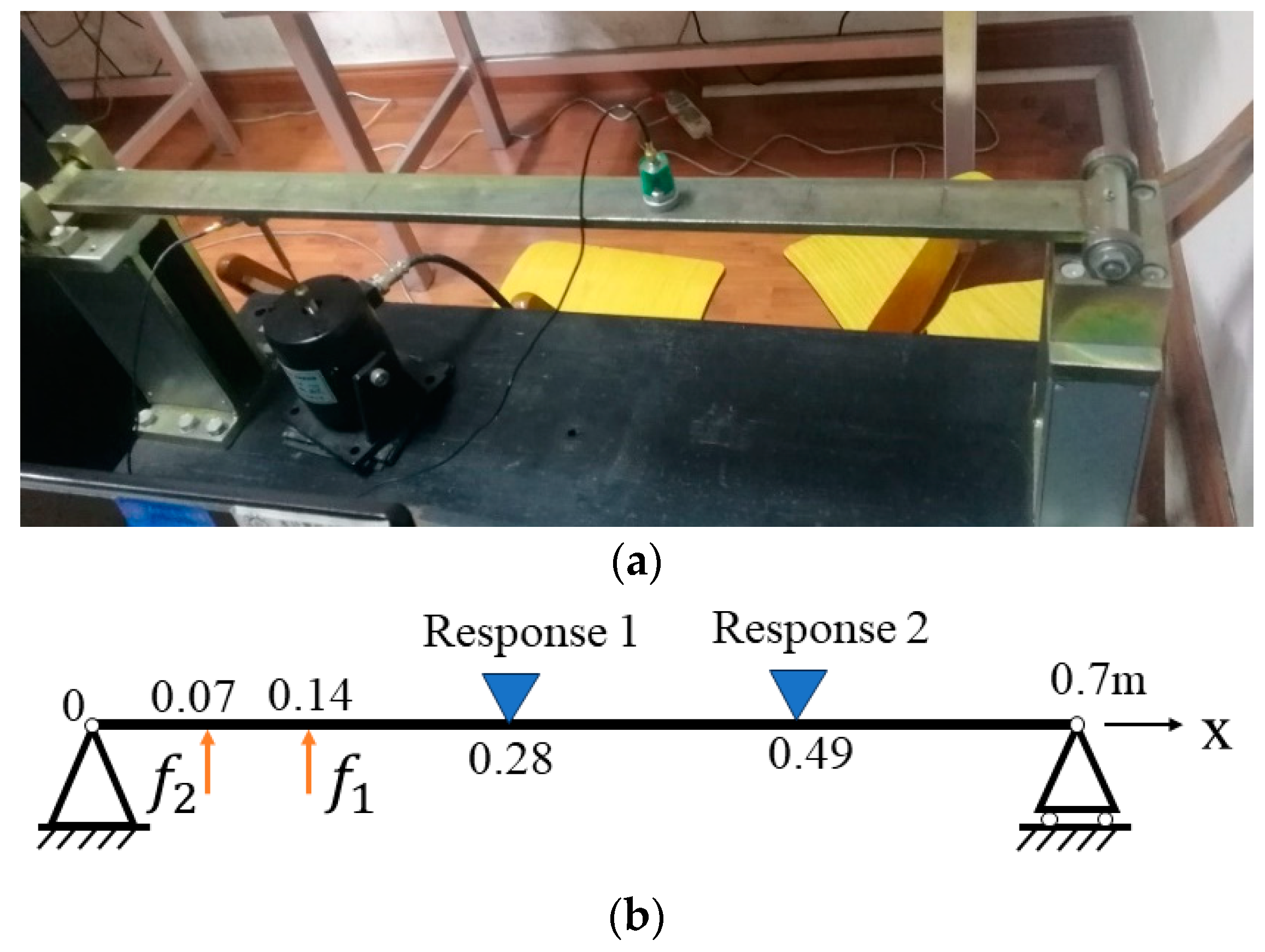
4. Experimental Verification

In this section, a simply supported beam, with a length of 0.7 m, width of 0.04 m, height of 0.008 m, elastic modulus of 210 GPa and density of 7850 kg/m³, was used to verify the FRF reconstruction model. The experimental model is shown in Figure 6.

Excitations $f_1\left(t\right)=\sin \left(40\pi t\right)$ and $f_2\left(2\right)=2\sin \left(80\pi t\right)$ were applied at 0.14 m from the left end of the beam simultaneously for single-point excitation, and then at 0.14 m and 0.07 m from the left end of the beam for multi-point excitation. Two accelerometers were placed at 0.28 m and 0.49 m from the left end of the beam. The frequency of response was obtained using Fourier transform, where ${\omega }_1$= 20 Hz and ${\omega }_2$ = 40 Hz. The positions corresponding to each frequency are shown in Figure 7 and

Table 8. Identification results.

Frequency (Hz)	Single-Source			Multi-Source
	Position (m)	Error (m)	%	Position (m)	Error (m)	%
${\omega }_1$	0.1394	0.0006	0.43	0.1394	0.0006	0.43
${\omega }_2$	0.1375	0.0025	1.79	0.0705	0.0005	0.36

.

In the case of the single-source and multiple frequencies, the result for the excitation position converged to 0.14, consistent with the actual excitation position. In the multi-source and multi-frequency case, the result for the excitation position converged to 0.14 and 0.07, consistent with the actual excitation position, too. The two response positions were consistent, so the number of excitation positions could be determined using the position corresponding to different frequencies.

5. Conclusions

A dynamic load position identification method based on FRF reconstruction is proposed in this paper.

(1)

By reconstructing FRFs, the objective function containing only the excitation position variable was established and solved. After the excitation position was identified, the error was assessed by comparing the amplitude and the phase of the solution with those of the real one.

(2)

This method can identify the locations of multiple loads with different frequencies, avoiding the ill-posed problem formulation caused by the traditional matrix inversion, identifying the excitation position quickly and accurately with a small amount of dynamic response information, and having a strong anti-noise ability.

(3)

When the same frequency data at different locations were used for the FRF reconstruction model, the method failed. So the data for different frequencies from measuring dynamic response should be selected to identify the load location for the FRF reconstruction model.

The simulation and experimental data demonstrate that this method can effectively identify the positions of dynamic loads.

References

1. Liu, R.; Dobriban, E.; Hou, Z.; Qian, K. Dynamic load identification for mechanical systems: A review. Arch. Comput. Methods Eng. 2022, 29, 831–863. [Google Scholar] [CrossRef]
2. Zheng, S.; Zhou, L.; Lian, X.; Li, K. Coherence analysis of the transfer function for dynamic force identification. Mech. Syst. Signal Process. 2011, 25, 22–29. [Google Scholar] [CrossRef]
3. He, Z.; Zhang, Z.; Li, E. Multi-source random excitation identification for stochastic structures based on matrix perturbation and modified regularization method. Mech. Syst. Signal Process. 2019, 119, 266–292. [Google Scholar] [CrossRef]
4. Turco, E. A strategy to identify exciting forces acting on structures. Int. J. Numer. Methods Eng. 2005, 64, 1483–1508. [Google Scholar] [CrossRef]
5. Hillary, B.; Ewins, D.J. The use of strain gauges in force determination and FRF measurements. In Proceedings of the 2nd International Modal Analysis Conference, Orlando, FL, USA, 6–9 February 1984; pp. 627–634. [Google Scholar]
6. Karlsson, S.E.S. Identification of external structural loads from measured harmonic responses. J. Sound Vib. 2003, 261, 329–349. [Google Scholar] [CrossRef]
7. Starkey, J.M.; Merrill, G.L. On the ill-Conditioned nature of indirect force measurements techniques. Int. J. Anal. Exp. Modal Anal. 1990, 8, 18–23. [Google Scholar]
8. Jacquelin, E.; Bennani, A.; Hamelin, P. Force reconstruction: Analysis and regularization of a deconvolution problem. J. Sound Vib. 2003, 265, 81–107. [Google Scholar] [CrossRef]
9. Gao, W.; Yu, K.; Gai, X. Application of L Norm fitting regularization method in dynamic load Identification of space-crafts. J. Vib. Shock 2017, 36, 101–107. [Google Scholar]
10. Wang, L.; Han, X.; Xie, Y. A new conjugate gradient method for solving multi-source dynamic load identification problem. Int. J. Mech. Mater. Des. 2013, 9, 191–197. [Google Scholar] [CrossRef]
11. Chen, Z.; Chan, T.H.; Nguyen, A. Moving force identification based on modified preconditioned conjugate gradient method. J. Sound Vib. 2018, 423, 100–117. [Google Scholar] [CrossRef]
12. Jiang, J.; Tang, H.; Mohamed, M.S.; Luo, S.; Chen, J. Augmented Tikhonov regularization method for dynamic load identification. Appl. Sci. 2020, 10, 6348. [Google Scholar] [CrossRef]
13. Liu, J.; Sun, X.; Han, X.; Jiang, C.; Yu, D. Dynamic load identification for stochastic structures based on Gegenbauer polynomial approximation and regularization method. Mech. Syst. Signal Process. 2015, 56, 35. [Google Scholar] [CrossRef]
14. Li, Z.; Feng, Z.; Chu, F. A load identification method based on wavelet multi-resolution analysis. J. Sound Vib. 2014, 333, 381–391. [Google Scholar] [CrossRef]
15. Gaul, L.; Hurlebaus, S. Identification of the impact location on a plate using wavelets. Mech. Syst. Signal Process. 1998, 12, 783–795. [Google Scholar] [CrossRef]
16. Alajlouni, S.; Albakri, M.; Tarazaga, P. Impact localization in dispersive waveguides based on energy-attenuation of waves with the traveled distance. Mech. Syst. Signal Process. 2018, 105, 361–376. [Google Scholar] [CrossRef]
17. Yu, W. Research on Load Location Identification Based on Directional Coupling; Harbin Engineering University: Harbin, China, 2018. [Google Scholar]
18. Zhang, J.; Zhang, F.; Jiang, J. Identification of dynamic load location based on variable separation method. J. Vib. Eng. 2021, 34, 584–591. [Google Scholar]
19. Zhang, C.; Li, J. Dynamic load identification and structural response reconstruction based on the augmented kalman filter. Appl. Math. Mech. (Chin. Ed.) 2021, 42, 665–674. [Google Scholar]
20. Li, Q.F.; Lu, Q.H. Impact localization and identification under a constrained optimization scheme. J. Sound Vib. 2016, 366, 133–148. [Google Scholar] [CrossRef]
21. Kazemi, M.; Hematiyan, M. An efficient inverse method for identification of the location and time history of an elastic impact load. J. Test. Eval. 2009, 37, 545–555. [Google Scholar]
22. Cao, X.; Sugiyama, Y.; Mitsui, Y. Application of artificial neural networks to load identification. Comput. Struct. 1998, 69, 63–78. [Google Scholar] [CrossRef]
23. Staszewski, W.J.; Worden, K.; Wardle, R.; Tomlinson, G.R. Fail-safe sensor distributions for impact detection in composite materials. Smart Mater. Struct. 2000, 9, 298. [Google Scholar] [CrossRef]
24. Shihan, H. Identification on Dynamic Load Position Based on Genetic Algorithm; Nanjing University of Aeronautics and Astronautics: Nanjing, China, 2020. [Google Scholar]
25. Yang, H.; Jiang, J.; Chen, G.; Zhao, J. Dynamic load identification based on deep convolution neural network. Mech. Syst. Signal Process. 2023, 185, 109757. [Google Scholar] [CrossRef]
26. Zhou, J.M.; Dong, L.L.; Guan, W.; Yan, J. Impact load identification of nonlinear structures using deep Recurrent Neural Network. Mech. Syst. Signal Process. 2019, 133, 106292. [Google Scholar] [CrossRef]
27. Qiu, B.B.; Zhang, M.; Li, X.; Qu, X.Q.; Tong, F.S. Unknown impact force localisation and reconstruction in experimental plate structure using time-series analysis and pattern recognition. Int. J. Mech. Sci. 2020, 166, 105231. [Google Scholar] [CrossRef]
28. Kulkarni, R.B.; Gopalakrishnan, S.; Trikha, M. Impact force identification in structures using time-domain spectral finite elements. Acta Mech. 2020, 231, 4513–4528. [Google Scholar] [CrossRef]
29. Wang, Y.; Zhou, Z.; Xu, H.; Li, S.; Wu, Z. Inverse load identification in stiffened plate structure based on in situ strain measurement. Struct. Durab. Health Monit. 2021, 15, 85–101. [Google Scholar] [CrossRef]
30. Zhu, D.; Zhang, F.; Jiang, J. Identification technology of dynamic load location. J. Vib. Shock 2012, 31, 20–23. [Google Scholar]
31. Zhu, D.; Zhang, F.; Jiang, J.; Zhang, W. Time-domain identification technology for dynamic load locations. J. Vib. Shock 2013, 32, 74–78. [Google Scholar]
Figure 1. Phase difference between dynamic responses.
Aerospace 10 00852 g001
Figure 2. Excitation f and response W on plate.
Aerospace 10 00852 g002
Figure 3. Contour lines of the correlation coefficient.
Aerospace 10 00852 g003
Figure 4. FRF reconstruction model.
Aerospace 10 00852 g004
Figure 5. Position error diagram for different levels of noise.
Aerospace 10 00852 g005
Figure 6. Experimental model (a) and excitation and response positions on it (b).
Aerospace 10 00852 g006
Figure 7. Single-source (a) and multi-source (b) positions.
Aerospace 10 00852 g007