Fluid-Dynamic and Aeroacoustic Characterization of Side-by-Side Rotor Interaction

Abstract

An investigation of twin corotating rotors’ interaction effects was performed by load (thrust and torque) measurements, flow field dynamics through Time-Resolved Particle Image Velocimetry, and acoustic emissions using a microphone array. Two rotors, each with a diameter of D = 393.7 mm and equipped with three blades, were investigated in a side-by-side configuration, to simulate a multirotor propulsion system. The mutual distance between the propellers is 1.02 D, and four different rotating speeds, i.e., 2620, 3500, 4360, and 5200 RPM, were explored. In such a configuration, thrust and torque undergo a reduction compared to that found for a single propeller configuration. The level of aerodynamic load fluctuations increases as well. The interaction of the wakes produces a recirculation region at the external periphery of the shear layers. An innovative approach involving the coupling of Proper Orthogonal Decomposition (POD) and Wavelet Transform has been employed to investigate the dominant structures within the flow and their mutual influence. The results reveal that the interacting wakes are dominated by a wave-like motion pulsating at Harmonics of the Blade Passing Frequency (HBPF) of 1/3. Higher orders of POD modes capture coherent vortical structures, including tip vortices pulsating at HBPF = 1. The aeroacoustic investigation shows that the noise level, in terms of the Over All Sound Pressure Level, presents a remarkable increment concerning that generated by the single propeller.

1. Introduction

Advances in inexpensive control systems and electronic devices have promoted the development of small Unmanned Aerial Vehicles (UAVs) in a wide range of applications [1]. Their unique ability to fly while hovering and maneuver highly, with vertical take-off and landing, makes UAVs extremely attractive. They offer promising solutions for several civilian applications, e.g., package delivery, field site surveillance, disease control, video taking, search and rescue, and personal entertainment. To provide sufficient thrust for small UAVs, the multirotor configuration has been extensively considered the most promising solution. Understanding the flow interactions between the rotors and the fuselage body remains an essential task for engineers who find optimality in terms of aerodynamic performances and the reduction of noise level. Therefore, the identification of noise sources significantly convinced the scientific community to study the phenomenon of rotor–rotor interaction in drones [2].

In the past years, studies of a single rotor have been conducted for the noise prediction of helicopters that typically fly at Reynolds numbers $Re\ge {10}^6$ [3]. These flow regimes differ from that established for drones, of the order of ${10}^4\le Re\le {10}^5$, which are equipped with blades of smaller sizes. Indeed, pressure fluctuations arise in transitional regimes, where Tollmien–Schlichting instability and a recirculation bubble are present [4].

Zhou et al. [5] studied the impact that produces the rotor-to-rotor interactions on the aerodynamic and aeroacoustic performances of small UAVs using load cells, microphones, and the Particle Image Velocimetry (PIV) experimental technique. They explored different distances between the rotors, observing increments of thrust fluctuations and noise levels as the distance downsizes. Unsteady loading was observed by Ko et al. [6] for a multirotor configuration inspected by numerical simulations. In hover, the wake interaction promotes asymmetries in the large-scale flow fields. Tinney and Sirohi [7] assessed the aerodynamic performance and the near-field acoustics of a multirotor drone comprising configurations, i.e., an isolated rotor, quadcopter, and hexacopter, for different propeller diameters. The acoustic near-field was inspected by an azimuthal array of microphones; they found that the sound pressure weakens as the propellers increase in number. In addition, a directivity pattern was observed associated with the blade pass frequency. Shukla and Komerath [8] carried out high-speed (400 Hz) Stereo PIV and performance measurements for two counter-rotating rotors placed side-by-side at different distances. The interaction becomes prominent for the closest configuration with a degradation of the aerodynamic performances. Stokkermans et al. [9] studied the wake interaction of two propellers in two different orientations, i.e., side-by-side and one after another, concerning the flow direction of the wind tunnel. They pointed out that the wake interaction strongly depends on the arrangement of the rotors with penalties in power when compensating for the thrust loss. Similar observations were outlined by Zanotti and Algarotti [10] for two propellers arranged in such a manner that their wakes overlap each other in wind tunnel tests. They argued that a partial overlap of propeller wakes determines acoustic drawbacks, as well as detrimental effects on aerodynamic performances.

Even though several studies on the interaction wake of multirotors in UAVs have been extensively conducted through experiments and numerical simulations, aeroacoustic aspects remain open issues in the scientific community. The wake interaction in multirotor UAVs undergoes a mutual rotor-to-rotor effect due to the close distance between the rotors [11]. The organization of the coherent structures embedded in the shear layers of both wakes plays a role in understanding their interaction [8]. Exploiting the periodicity of the shedding of the tip vortices, Zhou et al. [5] described the spatial organization of the tip vortices traveling in the shear layer. As expected, the vortex interaction undergoes significant dissipation effects due to their different convective velocity. Hence, the dynamic behavior inherent to the evolution of the tip vortices needs high-resolution measurements in both space and time.

In hover and without any significant geometric asymmetry of UAV configuration, it is reasonably assumed the multirotor configuration is a pair of rotors placed side-by-side. Hence, a basic understanding of the phenomenon of interaction wake is represented by studying one pair of rotors in side-by-side configurations.

In this study, two rotors in a side-by-side configuration and corotating have been operated by retaining fixed the rotor-to-rotor distance and by varying the rotational speed in a typical range for drone applications. The corotating rotor rotation direction was selected because this work originated as a study for distributed propulsion [12,13]. The specific rotor spacing of 1.02 D was chosen to amplify the effects of the interactions. This allowed the results to be more clearly visualized through the analyses performed. Load measurements have been carried out for the aerodynamic characterization of the two rotors. To unveil the dynamic features of the flow field at the interface of the interacting wakes, Time-Resolved PIV (TR-PIV) measurements (2.16 kHz) have been performed. A Proper Orthogonal Decomposition (POD) analysis based on the velocity field has been carried out to unveil the most dominant coherent structures. Turbulent flows, such as wake flows, are difficult to characterize due to their large range of spatial and temporal scales. Moreover, an innovative approach that holds great potential for studying highly time-dependent phenomena is presented. The Wavelet Transform (WT) is applied to the temporal coefficients derived from the POD, enabling the investigation of the dynamics of the most energetically significant phenomena. The overall dynamics can be reconstructed as a superposition of these effects. An additional experimental investigation in a semianechoic chamber in hover has been performed to acoustically analyze the effects of rotor-to-rotor interaction at the far field. An investigation of the noise pattern has been presented in terms of the Over All Sound Pressure Level (OASPL) in directivity form. Finally, a spectral analysis of aeroacoustic results has been carried out to highlight matching with the fluid-dynamic results expressed in the frequency domain.

2. Theoretical Background

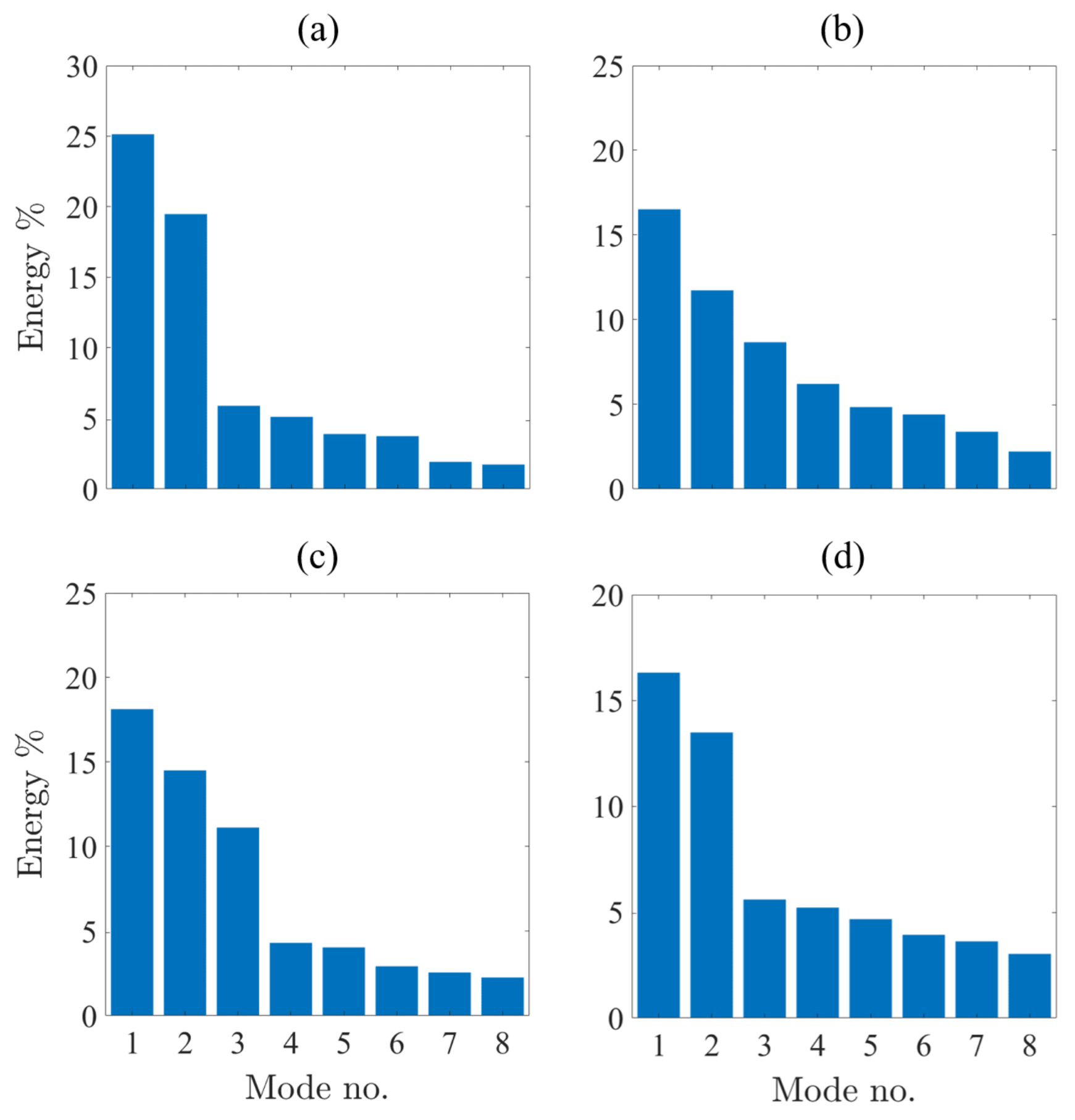
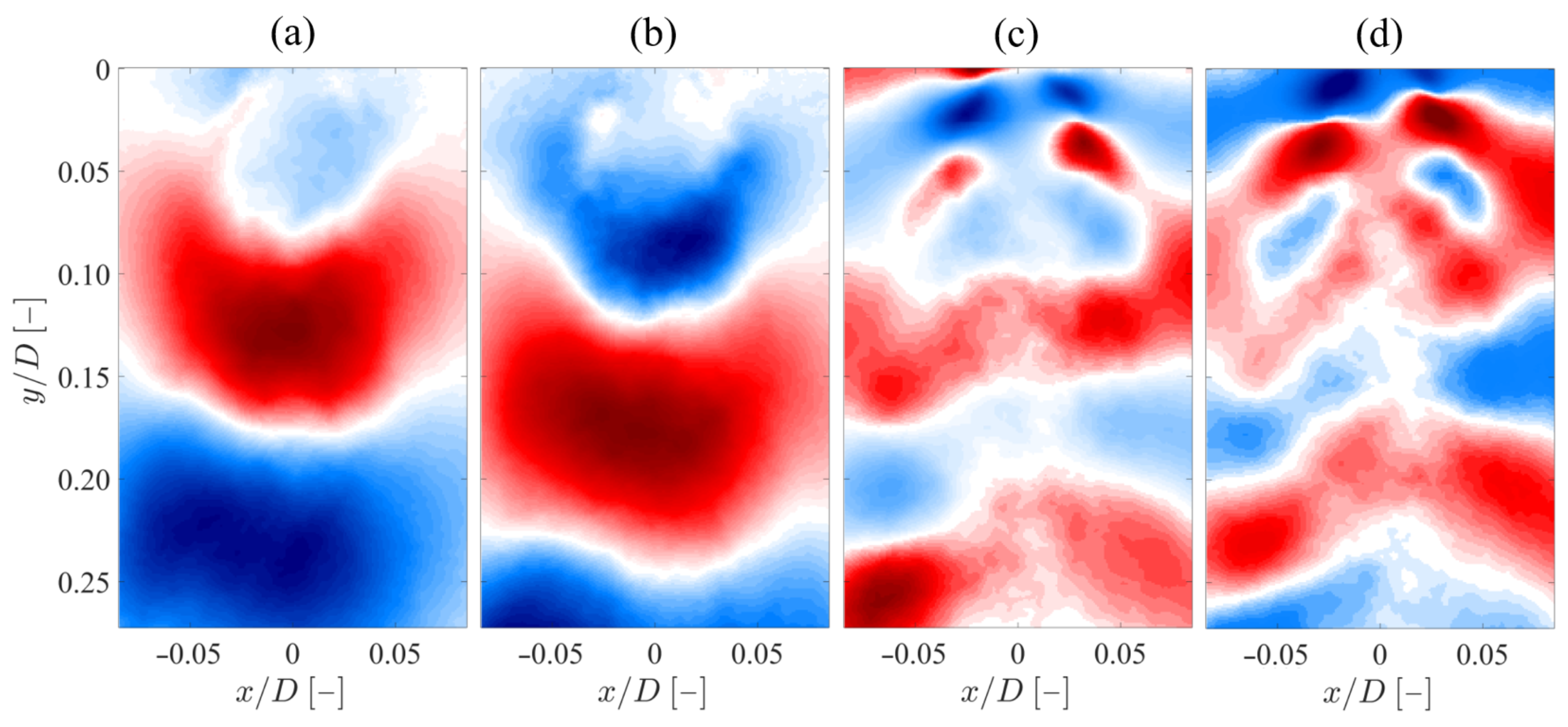
2.1. Proper Orthogonal Decomposition

The POD is a mathematical procedure, first introduced by Lumley [14], which exploits an orthogonal transformation to extract a set of bases from an ensemble of signals. It provides an energy-efficient decomposition through the principal components that are energetically sorted [15,16,17]. In addition, it does not require any assumption of linearity of the problem under investigation, making it very appealing for the analysis of fluid-dynamic fields. The bases represent an optimum for the ensemble, providing a unique decomposition. This technique uses second-order statistics in order to extract an organized large-scale structure from turbulent flows. The most energetic modes highlight the dominant flow structures [18,19].

Herein, the analysis is based on the Snapshot POD method [20,21], considering an amount of 600 PIV realizations for each case.

A preliminary step is to apply the Reynolds decomposition to the velocity vector:

$$\mathbf{U}(\mathbf{X},t)=\overline{\mathbf{U}}\left(\mathbf{X}\right)+\mathbf{V}(\mathbf{X},t),$$

(1)

where the overbar indicates the operation of the time-averaging; X and t represent the spatial and time coordinates, respectively.

The fluctuating components are organized in a matrix $\underline{\mathbf{V}}$, called the Snapshot Matrix:

$$\underline{\mathbf{V}}=\left[{\mathbf{V}}_1{\mathbf{V}}_2\cdots {\mathbf{V}}_M\right],$$

(2)

where N is the number of snapshots and each vector ${\mathbf{V}}_i$ is composed by the M element comprising the fluctuating velocity vector.

The two-point temporal Autocorrelation Matrix reads as follows:

$$\underline{\mathbf{C}}={\underline{\mathbf{V}}}^T\underline{\mathbf{V}}.$$

(3)

Then, the procedure is to resolve the corresponding eigenvalue problem:

$$\underline{\mathbf{C}}{\mathbf{A}}_i={\lambda }_i{\mathbf{A}}_i,$$

(4)

and to reorder the obtained solutions by the size of the obtained eigenvalues:

$${\lambda }_1>{\lambda }_2>\dots >{\lambda }_N.$$

(5)

The eigenvectors of Equation (4) comprise the basis of the POD modes ${\mathit{\phi }}_{\mathit{i}}\left(\mathbf{X}\right)$, which are retrieved by projecting the velocity fluctuation $\mathbf{V}(\mathbf{X},t)$ into the temporal structure $a_i\left(t\right)$ scaled by the amplitude $\sqrt{{\lambda }_i}$:

$${\mathit{\phi }}_{\mathit{i}}\left(\mathbf{X}\right)=\frac{1}{\sqrt{{\lambda }_i}}\sum _{n=1}^N\mathbf{V}(\mathbf{X},t_n)a_i\left(t_n\right),$$

(6)

where the sum is calculated over the time coordinate t.

Thus, each snapshot can be expressed by a sum of POD modes with coefficients $a_i$, named time coefficients. The time coefficients are defined as the projection of the velocity fields fluctuating partly onto the POD modes:

$$\mathbf{a}={\underline{\mathit{\varphi }}}^T\mathbf{V},$$

(7)

where the matrix $\underline{\mathit{\varphi }}$ is composed of the POD modes as $\underline{\mathit{\varphi }}=\left[{\mathit{\phi }}_1{\mathit{\phi }}_2...{\mathit{\phi }}_N\right]$. The total kinetic energy of the velocity fluctuating component of a single snapshot is proportional to the eigenvalue ${\lambda }_i$. In the case of periodic flow, the first few modes can capture most of the turbulent kinetic energy associated with them.

2.2. Wavelet Transform

Wavelet analysis is a tool for the study of localized variations of power embedded in a time series [22,23]. The WT permits expanding space/time history on a large variety of suitable functions, this feature makes it very interesting in a huge range of applications [24,25,26]. One of the main properties of WT is its duality in both time and frequency domains allowing for determining both the dominant modes of variability and how those modes vary in time.

In order to carry out a Continuous Wavelet Transform (CWT), the first step is the choice of a proper wavelet function, called the mother wavelet $\psi \left(t\right)$. The $\psi \left(t\right)$ can be real or complex. In this study case, the used mother wavelet is the Morlet function, which is a complex function, defined as follows:

$$\psi \left(t\right)={\pi }^{-1/4}{e}^{i{\omega }_{0}t}{e}^{-t^2/2},$$

(8)

where t is the dimensionless time and ${\omega }_0$ is the wavelet frequency center.

Starting from the mother wavelet $\psi$, a family of continuously translated and dilated wavelets (the orthogonal basis function) can be generated and normalized in energy norm:

$${\psi }_{s,\tau }=s^n\psi \left(\frac{t-\tau }{s}\right),$$

(9)

where s and $\tau$ are two real positive numbers called scaling parameter and time shifting, respectively. By varying the s and $\tau$, it is possible to represent the amplitude of any features versus the scale and how this amplitude varies with time in a single picture. In this present study, the L-2 normalization has been applied on the mother wavelet since, in Equation (9), $n=-\frac{1}{2}$ and

$${\int }_{-\infty }^{\infty }{∥{\psi }_{s,\tau }∥}^{2}dt=1.$$

(10)

Finally, the CWT is defined as follows:

$$w(s,\tau )=s^{-1/2}{\int }_{-\infty }^{\infty }x\left(t\right){\psi }^{*}\left(\frac{t-\tau }{s}\right)dt,$$

(11)

where $w(s,\tau )$ is the wavelet coefficient and ${\psi }^{*}$ is the complex conjugate of the dilated and translated mother wavelet function.

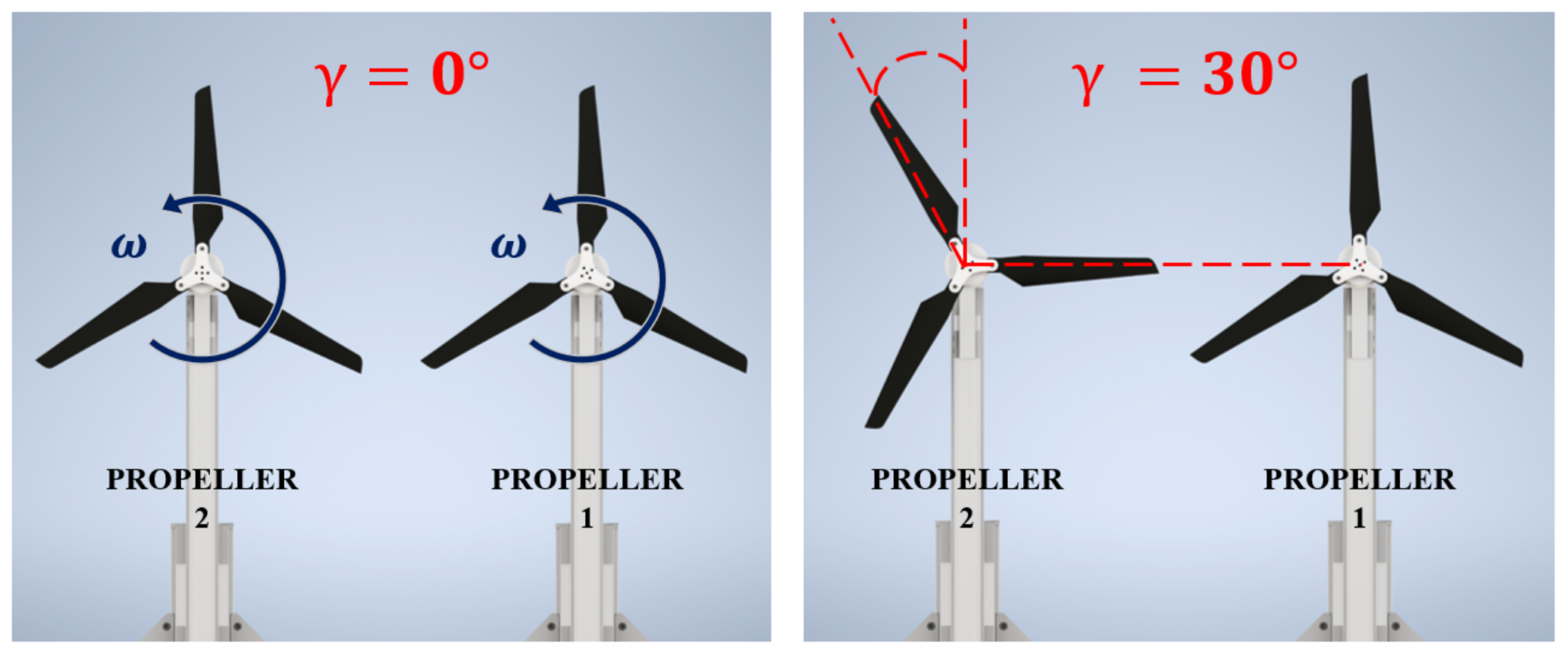
3. Experimental Setup

Two distinct measurement campaigns have been performed: one aimed at the aerodynamic and fluid-dynamics characterization of the rotor–rotor interaction and one for the study of its acoustic emissions. The first was conducted at the Aerodynamic Measurement Methodologies Laboratory, while the last was conducted at the CIRA semianechoic chamber. For the sake of clarity, we want to specify that the measurements were not carried out simultaneously to avoid any possible contamination of the acoustic chamber by the insemination material used for the TR-PIV measurements. For this experiment, a rotor test rig was designed and manufactured. Three bladed propellers, type KDE-CF155-TP (15.5″ × 5.3), were mounted on a custom-made horizontal support in order to perform Time-Resolved PIV (TR-PIV) measurements to investigate the evolution and spatial organization of the flow structures in twin-rotor wakes. The rotor characteristics were a diameter of $D=393.7$ mm and a chord of $c=28.5$ mm. Considering that the blade was tapered and swept, c was referred to as the mean aerodynamic chord (MAC). The resulting rotor solidity value was equal to $\sigma =0.138$. The rotor solidity is defined as

$$\sigma =\frac{BcR}{A}=\frac{Bc}{\pi R},$$

(12)

where B is the number of the blades of propeller, c is the mean aerodynamic chord, R is radius of the propeller, and A is the rotor disk area.

The complete description of the blade characteristics is illustrated in Figure 1 in terms of radial distributions of chord $c/R$, normalized thickness $T_{hk}/c$, and blade pitch $\beta$.

Each rotor was driven by a KDE4012XF-400 motor and a KDEXF-UAS55 electronic speed controller. Dedicated software in the NI LabVIEW 2017 environment has been developed to control the rotation speed. The twin propellers were placed such that the reciprocal distance between the rotor axes was $d=1.02$ D. The rotor disks had a distance from the floor of $H=4.37$ D to avoid any presence of ground effect. The twin-rotor was operated in hover conditions at four different propeller speeds, respectively, at ${\mathrm{\Omega }}_1=2620$ RPM, ${\mathrm{\Omega }}_2=3500$ RPM, ${\mathrm{\Omega }}_3=4360$ RPM, and ${\mathrm{\Omega }}_4=5200$ RPM. The rotational speed was measured by using a Kubler 05.2400 incremental encoder characterized by 500 $ppr$ (pulses per revolution).

The test conditions, i.e., the tip velocity, Mach number at the blade tip, and Reynolds number calculated at $75\%$ of the propeller radius, are summarized in

Table 1. Test conditions at the explored propeller speeds: tip velocity $U_{tip}$, Mach number $M_a$ at the blade tip, and Reynolds number at 0.75R.

$\mathbf{\Omega }$ (RPM)	${\mathit{U}}_{\mathit{tip}}$ (m/s)	${\mathit{M}}_{\mathit{a}}$ (−)	$\mathit{R}\mathit{e}$ (−)
2620	54	0.157	$6·{10}^4$
3500	72	0.210	$8·{10}^4$
4360	90	0.262	$1·{10}^5$
5200	107	0.313	$1.2·{10}^5$

. The tip velocity was calculated as follows:

$$U_{tip}=\frac{2\pi \mathrm{\Omega }R}{60}.$$

(13)

To measure the propeller aerodynamic loads, the Kubler encoders were removed and the motors were fixed to the six-component force and torque load cells, using tailored interface plates (Figure 2). The second propeller was mounted on a dummy balance to preserve the symmetry of the rotor rig. The balance was an ATI Mini 40 model characterized by full-scale values and the accuracy is indicated in

Table 2. Balance characteristics.

	${\mathit{F}}_{\mathit{x}}$ (N)	${\mathit{F}}_{\mathit{y}}$ (N)	${\mathit{F}}_{\mathit{z}}$ (N)	${\mathit{M}}_{\mathit{x}}$ (Nm)	${\mathit{M}}_{\mathit{y}}$ (Nm)	${\mathit{M}}_{\mathit{z}}$ (Nm)
Full scale	±20	±20	±60	±1	±1	±1
Accuracy (% FS)	0.25	0.25	0.60	0.0125	0.0125	0.0125

. The measurements were carried out at a sampling frequency of 1000 Hz for a time of 20 s. The mean force and moments were evaluated together with the standard deviation.

The lack of the encoder decreased the accuracy of controlling the rotational speed. A single microphone in the proximity of the propellers monitored the rotational speed. The microphone was a Gras model 40PK CCP. The microphone data were acquired at a sampling frequency of 51,200 Hz for 30 s. Simultaneously, a single hot film probe was located above the propeller disc at about $z=+32\mathrm{mm}$ and at a radial distance of 0.62 R for monitoring the inlet flow qualities and crosschecking the rotating speed.

The wake interaction of the twin rotors was inspected by TR-PIV measurements, planar bi-dimensional and two components (see Figure 3), at an acquisition frequency of 2160 (double frames per second). This enables capturing either 49 images per revolution at ${\mathrm{\Omega }}_1=2620$ RPM or 25 images at the highest speed of ${\mathrm{\Omega }}_4=5200$ RPM. The setup was composed of a Photonics DM 30 dual-head Nd-YLF laser with an average power value of 45 W at a maximum repetition rate of 3 kHz. At the operating frequency of $2.16$ kHz, the laser provided a pulse energy of about 20 mJ per pulse at the wavelength of 527 nm. A system of three high-speed cameras was installed consisting of two Phantom VEO 710L (7400 frame rate, 1280 × 800 pixels, 12-bit, pixel dimension 20 $\mathsf{\mu }$m) and one Phantom VEO 640L (1400 frame rate, 2560 × 1600 pixels, 12-bit, pixel dimension 10 $\mathsf{\mu }$m). In order to fully exploit the operative laser repetition rate, the VEO 640 was operated to the resolution of 1280 × 800 px. In order to track the blade tip vortices in the proximity to the rotor disk, the two VEO 710 cameras were equipped with a Nikkor lens featuring a fixed focal length of 200 mm, and the f-number was set to $f\#=5.6$ while the VEO 640 used a Zeiss lens with a fixed focal length of 100 mm and the f-number was set to $f\#=2.8$. Since the flow field investigation focuses on the wake interaction and tracking the embedded coherent structures, it is evident that the inspected region covers a relatively small area. The sight view of the upper camera was orthogonal to the laser plane; the lower cameras were slightly tilted with respect to the plane. For the latter cameras, Scheimpflugh systems were used to avoid the out-of-focusing of the lateral regions.

The origin of the reference system was placed at the middle distance between the rotor axes, with the x-axis laying horizontally along the rotor disk plane, the y-axis in the direction of the thrust vector, and the z-axis following the right-hand rule (Figure 4). The measurement region was located immediately below and between the two propeller disks on a vertical plane radially ranging between $x/D=-0.115$ and $x/D=0.125$. The size of the Field of View (FOV) covers an area of 90 × 130 mm${}^2$. In order to follow the wake interaction, all cameras were mounted horizontally and the Region of Interest was partially overlapped. The three-camera imaging was stitched together, covering a vertical region from $y/D=-0.075$ to $y/D=0.27$.

In addition, Figure 4b shows the propellers’ clearances from the support structures. This distance allows the support to not affect the wakes. Instead, the arm supporting the motor is perfectly compatible with the drone geometries.

The image calibration and perspective distortion correction of the three cameras were performed using a 3D calibration plate having two planes spaced by 2 mm. The pinhole camera model was used for the calibration and distortion correction [27]. This yielded a spatial resolution of about 17.3 px/mm in the image plane. The separation time between the laser double-pulses ranged between 40 and 60 $\mathsf{\mu }$s according to the propeller revolution speed. As tracer particles, aerosolized diethylhexylsebacate (DEHS) oil was used. A seeding generator with 20 Laskin nozzles provided oil droplets with a size of less than 1 $\mathsf{\mu }$m. The full test room was seeded in order to have a homogenous concentration of particles. The PIV images were preprocessed by applying a background gray-level subtraction. Davis 10.1 (by LaVision) was used to record and process the particle images. The particle images were further preprocessed using sliding background subtraction and a particle intensity normalization in sliding windows of $5\times 5\mathrm{px}$ to account for inhomogeneities in the laser light sheet and the varying particle intensity. The analysis consisted in an iterative multipass cross-correlation algorithm ending at $24\times 24{\mathrm{px}}^2$ and a $75\%$ overlap [28,29]. The subpixel accuracy for the detection of the correlation peak was obtained by using a three-point Gaussian fit [30].

The results presented a velocity spatial resolution of $\Delta x=0.46$ mm. The random noise from the cross-correlation procedure can be preliminarily estimated as 0.1 px as a rule-of-thumb [31]. Using the current values for the optical resolution (17.3 px/mm), having the laser double-pulse delay (from 40 $\mathsf{\mu }$s to 60 $\mathsf{\mu }$s), the uncertainty related to a velocity field ranges between $\Delta V$ = 0.14 and 0.09 m/s.

In order to analyze the mutual rotor-to-rotor interactional effects on the far field of the pressure fluctuations, acoustic measurements were performed within a semianechoic chamber. A new support of the test rig was designed and implemented for this purpose. The propeller discs were vertically oriented and the rotating axes were placed at a height of 1.5 dm from the ground. The rotor rig was placed in the center of the CIRA semianechoic chamber with dimensions equal to 5.65 $\left(L\right)$× 4.45 $\left(W\right)$× 4 $\left(H\right)$ m${}^3$ and characterized by a cut-off frequency equal to 90 Hz (Figure 5). An array of eight microphones, the G.R.A.S. 40PK CCP model, was placed at a distance of 5 D from the midpoint of the two rotors, constrained on a semicircular modular structure, realized in rapid prototyping. The azimuthal spacing $\Delta \theta$ between the microphones was ${10}^{\circ }$.

To encompass the circumference surrounding the rotors through the so-built microphone array, this latter was translated along the azimuthal direction covering a total of five positions (Figure 6). A NI LabVIEW software was implemented to acquire pressure data by using two NI 9234 modules of 4 channels each. Data were acquired at a sampling frequency of 51,200 Hz for 30 s.

Finally, the pressure signals were filtered with a band-pass filter, over the frequency range from 90 Hz to 20 kHz. The first frequency value, 90 Hz, is the cutoff frequency of the semianechoic chamber, and 20 kHz is the maximum frequency that can be acquired by microphones (also corresponding to the maximum value audible to the human ear).

4. Results and Discussion

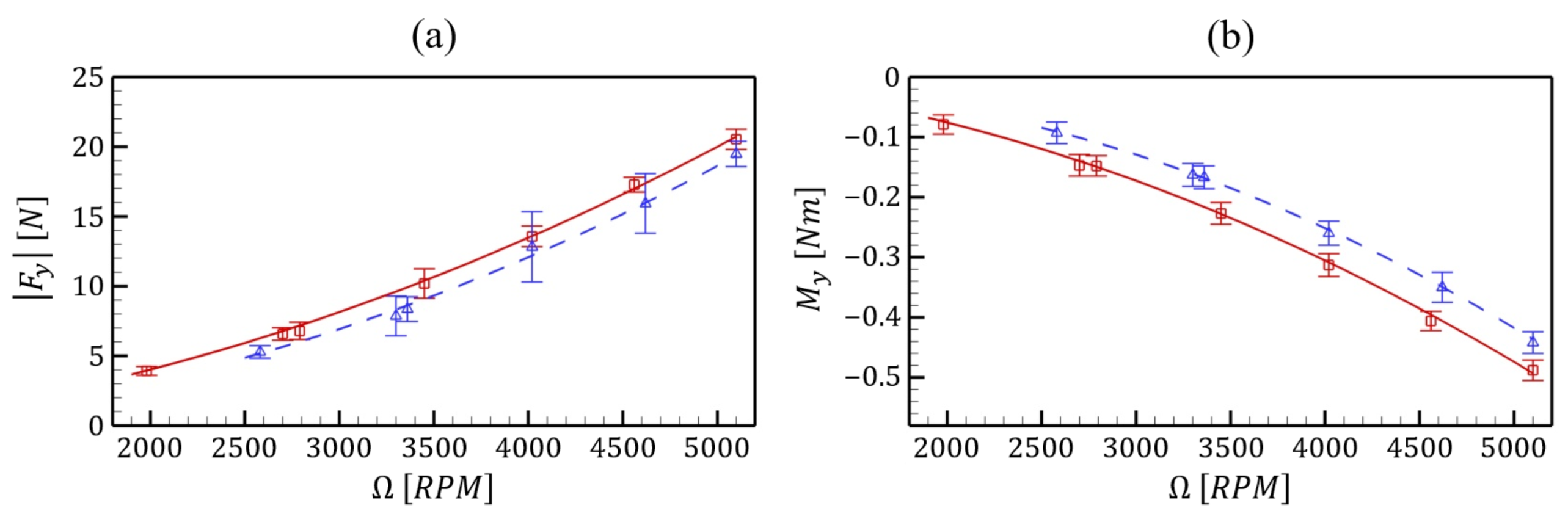
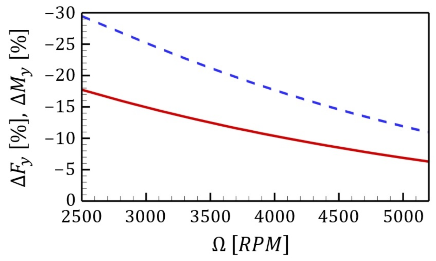
4.1. Dynamic Load Characterization

The propeller aerodynamic performances have been investigated for isolated and tandem configurations varying the rotating speed. For the isolated propeller, the mean values over 20 thousand samples of the thrust ($F_y$) and torque ($M_y$) are plotted versus the rotating speed (Figure 7a,b red markers). The trend of thrust and torque indicates growth in terms of absolute values as the rotational speed ($\mathrm{\Omega }$) increases. Both follow a second-order polynomial law. The corresponding standard deviation of the acquired data is plotted in terms of error bars.

The side-by-side configuration presents a reduction in thrust for the complete velocity range and a remarkable increment in force fluctuation (i.e., thrust standard deviation) compared to the single rotor case. The force fluctuation increases up to $20\%$ of the average value compared to a value of $3\%$ for the single rotor. This agrees with previous works. A thrust coefficient reduction of $2\%$ was presented by Zhou et al. [5] for twin propellers at a distance of $d=1.05$ D, with a remarkable increment of the force fluctuation. Also, Chen et al. [32] measured the thrust reduction of the order of $5\%$ for the Disk Loading of $DL=45$ N/m${}^2$ and a distance of $1.025$ D and claimed that the percentage loss of thrust was directly influenced by the Disk Loading; the more the propeller is loaded, the greater the loss of thrust. The wake interaction affects the torque values with a decrease in terms of absolute values throughout the whole speed range. The torque fluctuations are similar to the single propeller case. Thus, in the case of the interaction between the two rotors, in addition to the thrust decrease, a reduction in torque is present, suggesting a blade drag reduction as well.

The thrust and torque difference values between the isolated propeller and the side-by-side propellers are plotted in terms of percentage values concerning the isolated propeller values (Figure 8). The data are obtained as $\Delta F_i=((F_{Ti}-F_{Si})/F_{Si})\ast 100$, where $F_{Si}$ is the i-components of the single propeller loads and $F_{Ti}$ is the i-components of the loads for the tandem configuration.

The thrust reduction indicates a value of $17.7\%$ at a speed of 2500 RPM until $5.5\%$, increasing the rotating speed at 5500 RPM. For a Disk Loading of 181 N/m${}^2$ at a rotating speed of 5200 RPM, a reduction of $6.3\%$ concerning the isolated propeller is encountered in agreement with the results presented by [5,32] (see Figure 8). The torque reduction varies from a value of about $30\%$ at $\mathrm{\Omega }=2500$ RPM to $9.5\%$ at a rotational speed of 5500 RPM.

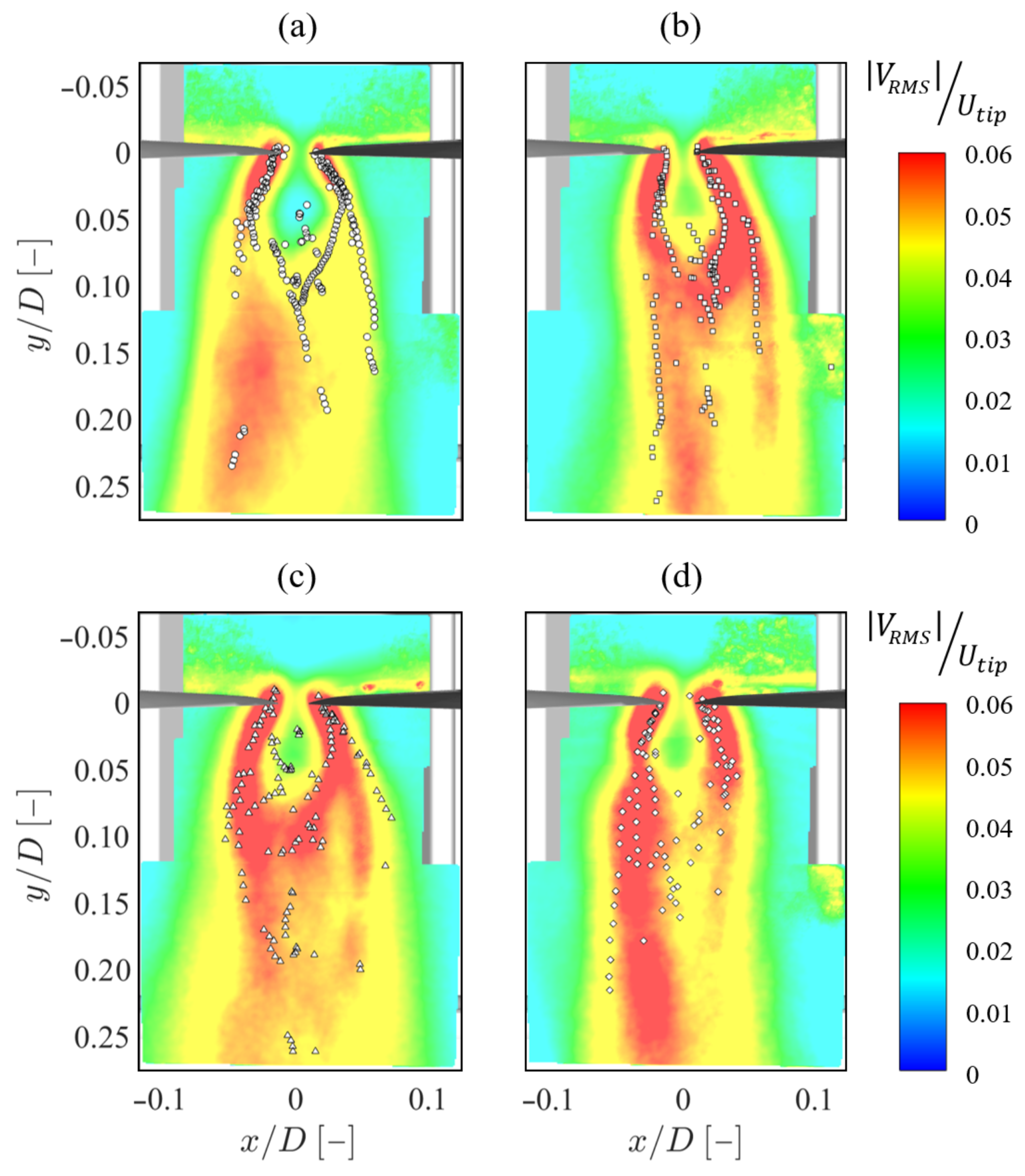
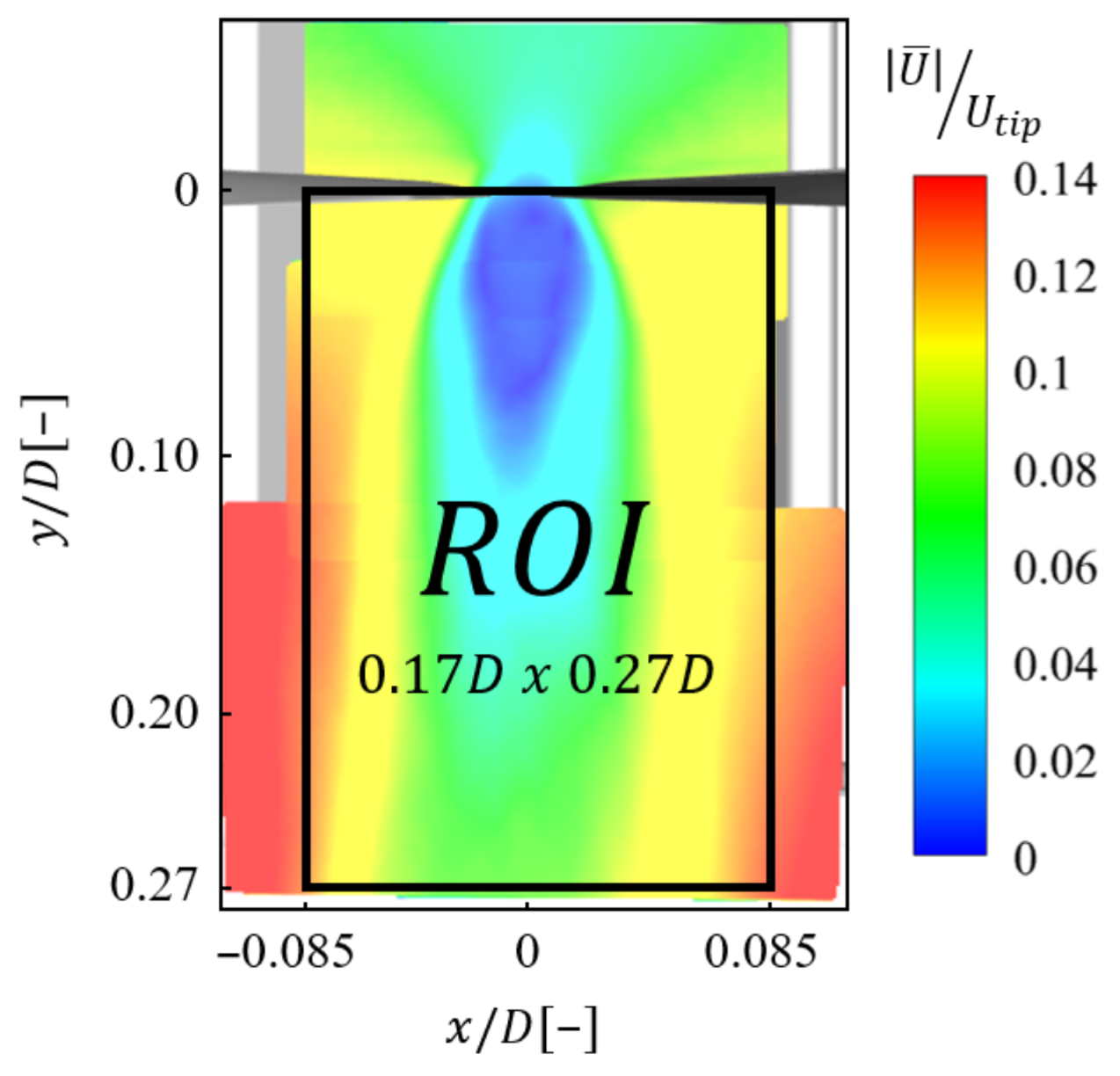
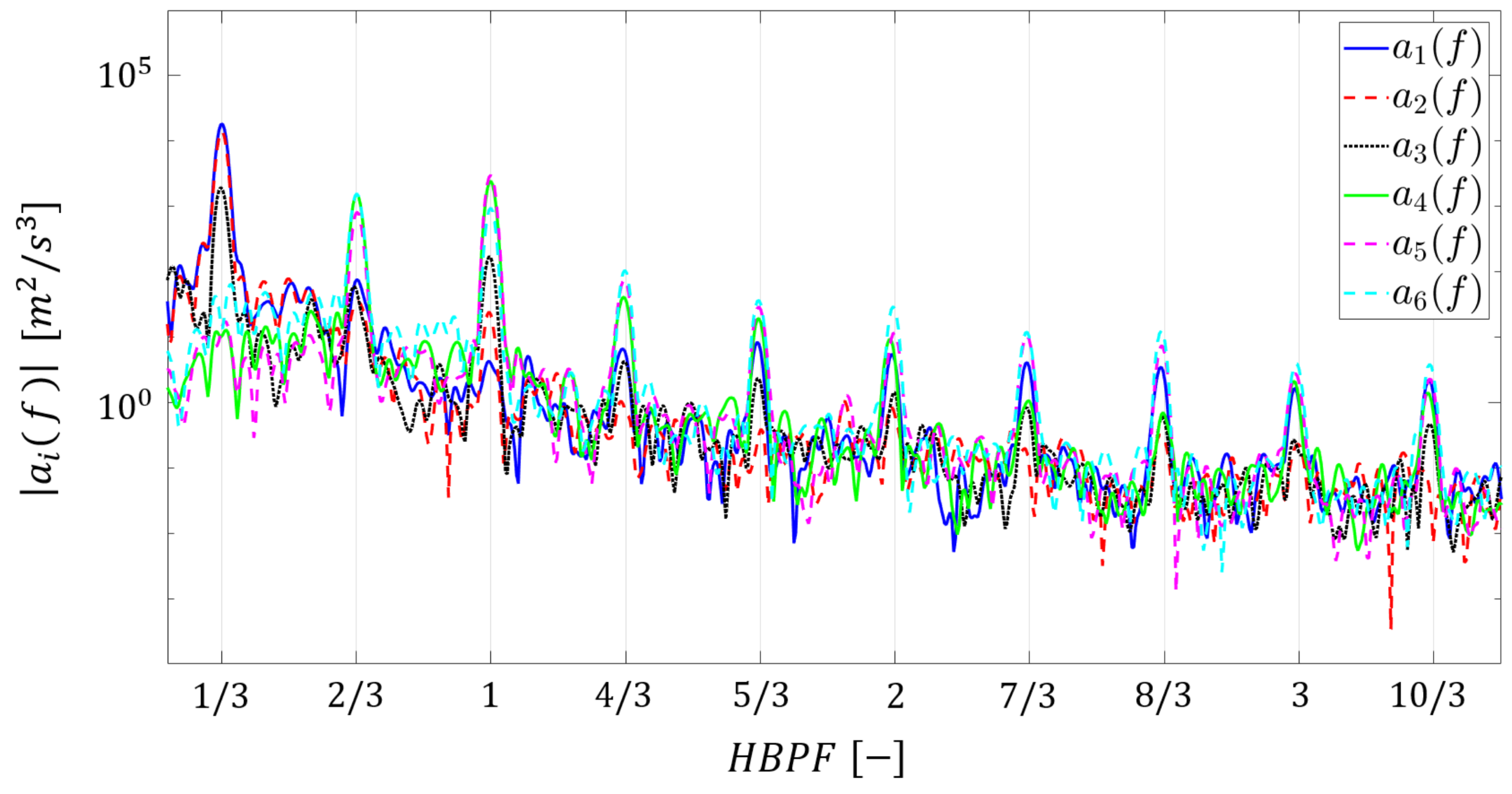
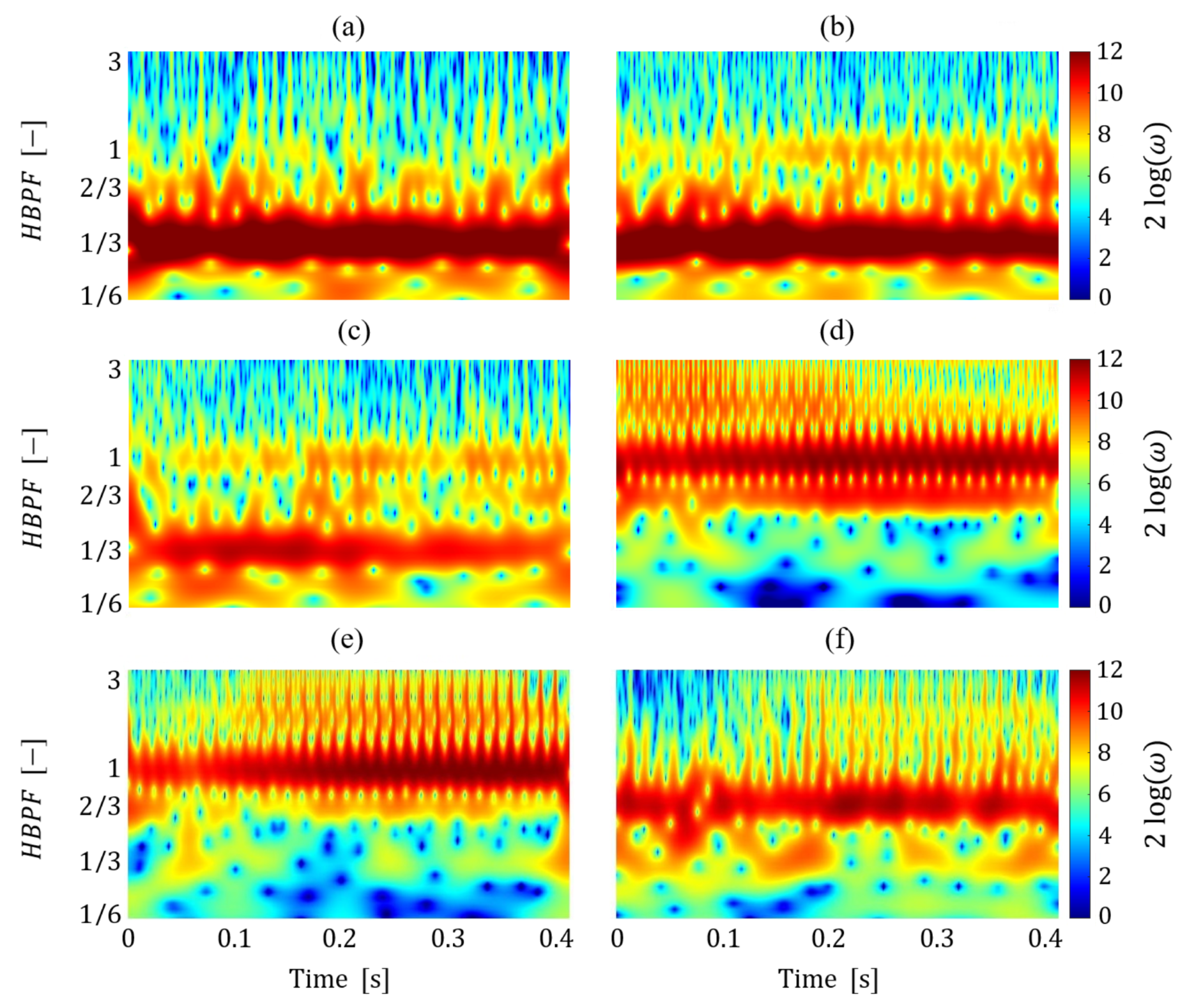
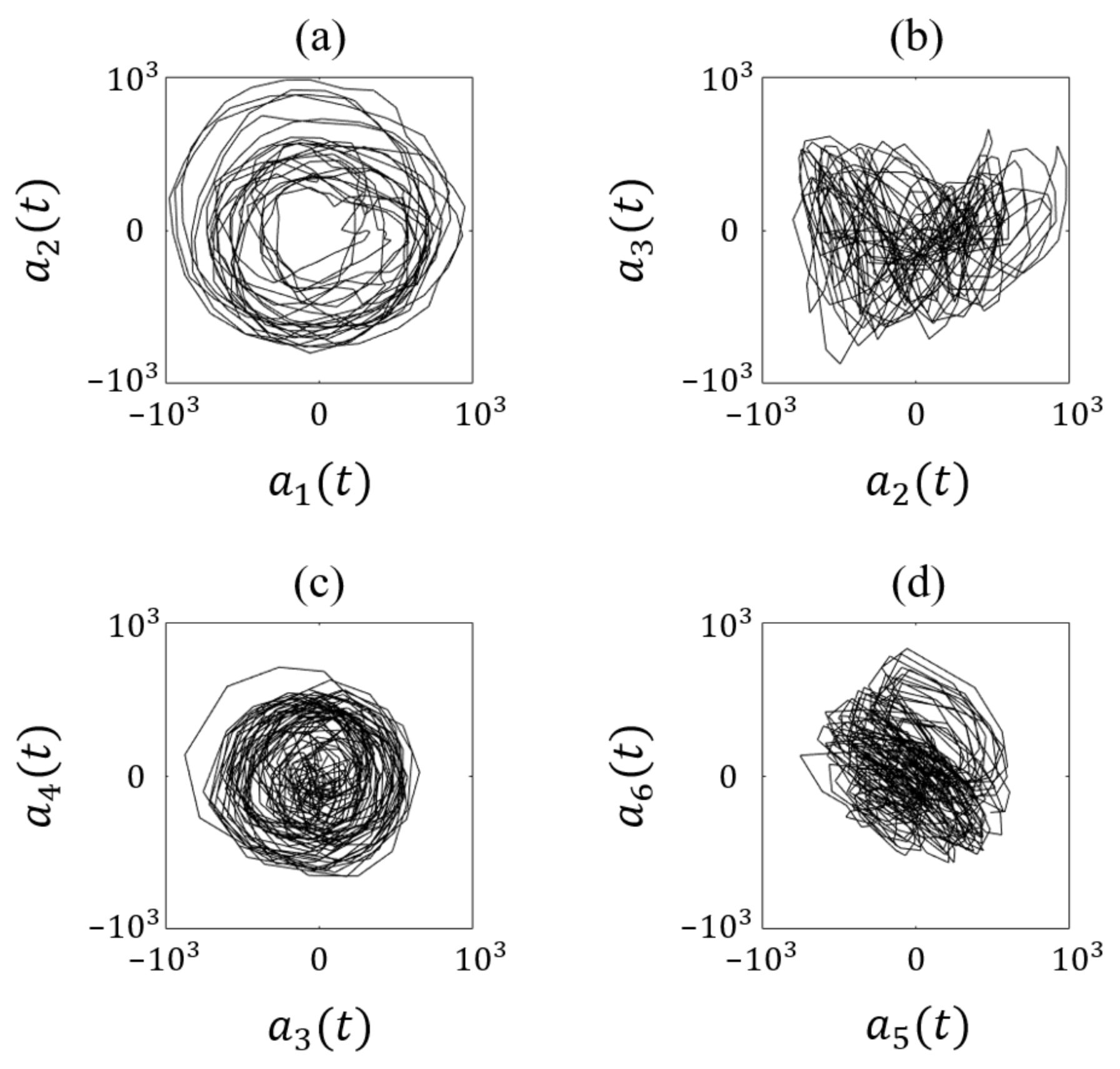
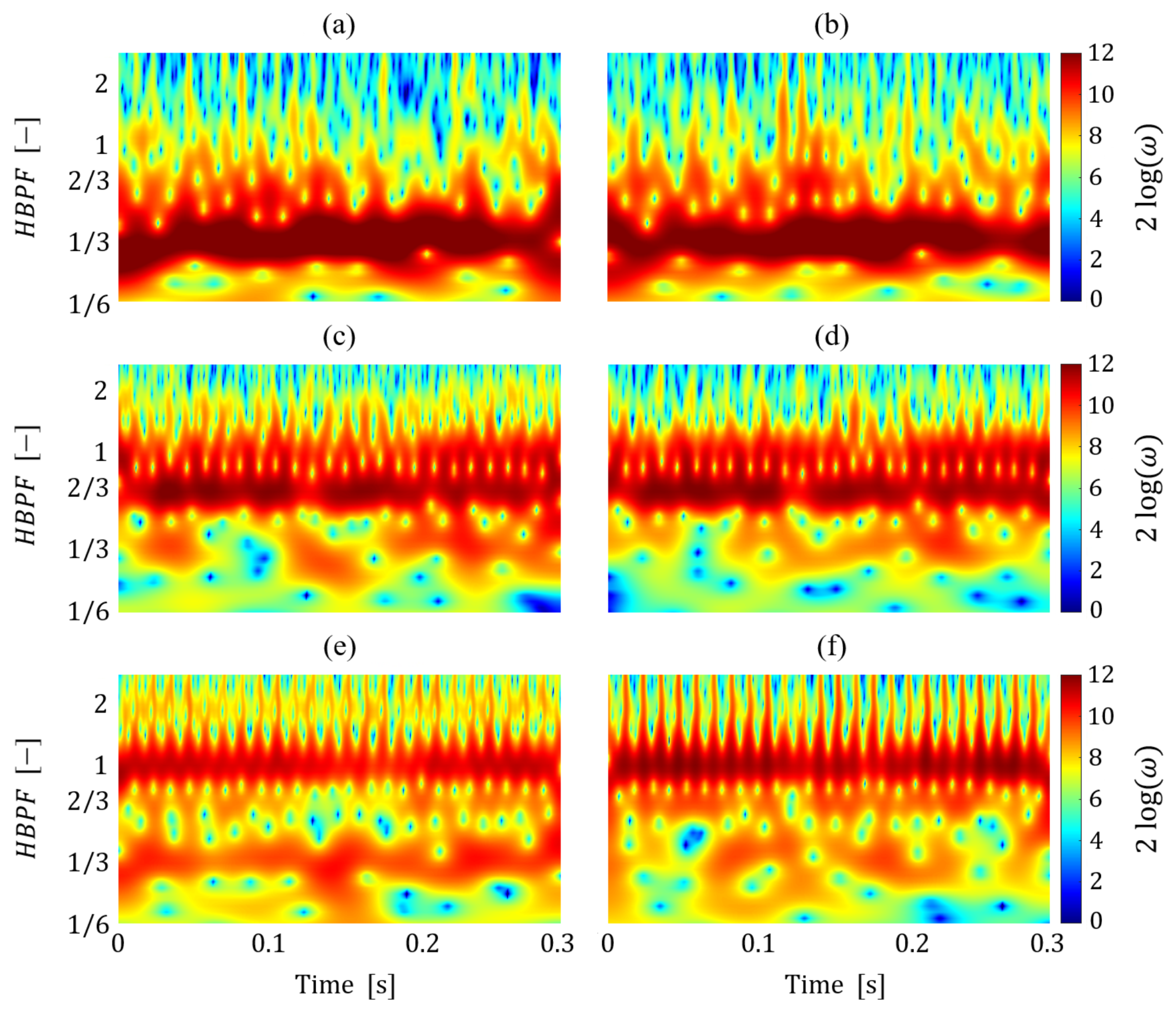
4.2. Flow Field Characterization

The wake interaction of the two rotors in a side-by-side configuration was explored by inspecting the flow fields, focusing on the main features of the time-average flow fields. In the following, the operation $\left|\mathbf{U}\right|$ is referred to as the modulus of the velocity vector. The results are reported in dimensionless form, using the characteristic velocity $U_{tip}$ and the rotor diameter D as the reference quantities. The time-averaging process has been computed over 575 time-resolved snapshots, at a minimum. In Figure 9, the isocontours of the time-average flow field color-coded with the dimensionless velocity magnitude $|\overline{U}|/U_{tip}$, superimposing the stream traces, are presented for the rotor speeds of $\mathrm{\Omega }=2620$ RPM (a), 3500 RPM (b), 4360 RPM (c), and 5200 RPM (d). On average, the flow patterns exhibit typical features of rotor wakes [8]. The contraction of the wakes dominates near the rotor discs. For each explored rotor speed, the wake interaction establishes low levels of velocity magnitude at the interface between the rotor wakes. From the visualization of the paths underlined by the stream traces, the maps exhibit the presence of multiple recirculation regions within the plane. Further downstream, the wakes lose the characteristic pattern of that found for a single rotor and the interaction produces the flattening of the shear layer directions. This resulting asymmetry of the flow patterns about the vertical axis suggests the presence of a mutual attraction that the wakes undergo when interacting with each other. This residual bias is more evident for the test case at 3500 RPM (Figure 9b), where the main flow deviates by ${12}^{\circ }$ with respect to the vertical direction. It is worth underlining that the relative azimuth position between the rotors can impact the wake interaction.

Since the rotor speed was maintained constant for both rotors, the phase angle $\gamma$ between them is considered fixed during the acquisition time and, eventually, is retrieved by the TR-PIV realizations. It has been defined as indicated in Figure 10, hence, in

Table 3. Phase angle $\gamma$ between the rotors.

Test Case (−)	$\mathbf{\Omega }$ (RPM)	$\mathit{\gamma }$ (deg)
1	2620	90
2	3500	20
3	4360	60
4	5200	90

, the resulting phase angles are reported. Interestingly enough, for Test Case 3, the phase angle attains ∼60${}^{\circ }$, which means that the blades of either rotor are synchronously imaged in the investigated region. This has an impact on the wake interaction testified by the map of Figure 9c; here, the stream traces denote the absence of any recirculation region at the interface of the rotor wakes. The vortical structures participating in the buildup of the flow are shed from the blade tip of either rotor, undergoing a repulsive approach that mitigates the recirculation effects. On the other hand, for all the other cases, the recirculation dominates at the initial interface $0\le y/D\le 0.1$, producing scattered patterns even with spatial asymmetries.

As already mentioned, the shear layers of both wakes embed vortical structures, in the literature referred to as tip vortices [33,34,35,36]. Their effects are addressed on average by mapping the magnitude of the root mean square (RMS) of the velocity fluctuations, $|V_{RMS}|/U_{tip}$, as illustrated in the isocontours of Figure 11. The locations of the vortical structures have been detected over each cycle through the method implemented by [37], based on the ${\mathrm{\Gamma }}_2$-criterion, first proposed by [38]. These have been superimposed on the maps of Figure 11 through white markers over five cycles indicating the scattering of their spatial organization. As expected, the velocity fluctuations exhibit peaks localized in the shear layer regions predominantly due to the passage of the tip vortices and in part by the turbulence of the wakes. From the inspection of the vortical locations, there are trajectories observed for all the inspected rotor speeds. In the proximity of the rotor disc, the trajectories overlap with each other, which indicates that no wake interaction occurs confirming the observations already discussed for the time-average velocity magnitude. The contraction, undergone by each wake, dominates for stabilizing the vortical paths along a preferred trajectory; this behavior can be found in isolated rotors as well [39]. Further downstream, the wake interaction gradually takes place, promoting the merge of the trajectories, and the scattering of the vortical locations becomes more significant. Interestingly enough, it is possible to recognize different preferred paths, taking place as bifurcations, as shown in the maps of Figure 11a–c. The level of the velocity fluctuations decreases when moving away from the rotor disc, and it spreads over the thickness of the shear layer. This effect has more impact at $\mathrm{\Omega }=4360$ RPM when being performed at a phase angle of $\gamma ={60}^{\circ }$ (Figure 11c). Asymmetries of the RMS of the velocity fluctuations are found for all the investigated rotor speeds.

The inspection of the energetically prominent large-scale flow structure is addressed by means of POD analysis, considering the radial component of the velocity field [40]. Even though clusters of outliers have been removed in the data post-processing, the velocity field is affected by spurious vectors localized at the regions where the propellers were imaged. This can compromise the POD analysis introducing a bias into the evaluation of the orthonormal bases. To overcome this issue, a resizing of the Region of Interest has been accomplished by focusing on the area where the wake interaction is prominent, as shown in Figure 12. A centered rectangle has been drawn with the upper side right below the rotor disc till downstream, with a horizontal size of $0.17$ D.

Since the POD analysis allows for the extraction of the most energetically relevant large-scale structures, they are captured by the orthonormal modes, and the associated energies are hierarchically presented in Figure 13 for all the rotor speeds. In Figure 13a, mode $\#1$ and $\#2$ capture approximately $25\%$ and $19.5\%$ of the total energy indicating a higher efficiency in the decomposition for $\mathrm{\Omega }=2620$ RPM, with respect to that observed for the other rotor speeds. This efficiency slightly reduces for $\mathrm{\Omega }=5200$ RPM, which collects in the first couple of modes $16\%$ and $13.5\%$, respectively. A smoother distribution of the spectral energy over the modes is observed for the remaining rotor speeds.

The spatial organization of the first four dominant POD modes is depicted in the maps of Figure 14 for $\mathrm{\Omega }=2620$ RPM. The first pair describes the wave-like motion of the wakes interacting with each other, as testified by the wavy pattern of the modes. Interestingly enough, they deviate from the representation of the tip vortices typically encountered in the decomposition of wakes generated by a single rotor [41]. The second pair identifies the typical organization of the tip vortices, captured in a narrow region right below the rotor disc, and then, downstream, they refer to a higher order of the wavy pattern (Figure 14c,d) already encountered for the first pair.

As already introduced in Equation (7), by definition, the time coefficients $a_i$ include information about the time correlation between the snapshots. Plotting their power spectra, the modes exhibit the pairing through the harmonics. Figure 15 shows the distribution of the Power Spectral Density of the first four-time coefficients captured at $\mathrm{\Omega }=2620$ RPM. They are plotted as a function of the Harmonics of the Blade Passing Frequency (HBPF), which is defined in Equation (14).

$$HBPF=\frac{60f}{B\mathrm{\Omega }}$$

(14)

As already mentioned, in Figure 15, there are pairs considering the peaks in the harmonics of the time coefficients of the POD modes 1–2 and 3–4. In particular, $a_1\left(f\right)$ and $a_2\left(f\right)$ reveal one at $HBPF=1/3$, which means that the wave-like motion of the interacting wakes pulsates at the rotor frequency. On the other hand, $a_3\left(f\right)$ and $a_4\left(f\right)$ reflect the shedding of the tip vortices evolving in the shear layers at $HBPF=1$, i.e., the blade passage frequency.

To verify that the first four modes represent coherent harmonics, comparison plots are depicted in Figure 16; the scattering of the time coefficients $a_i\left(t\right)$ of the individual realization is illustrated for different combinations. In Figure 16a,d, the time coefficients are located in the neighborhood of a circumference, thus indicating the periodicity of the large-scale flow structures captured by the pairs. The crosstalk between the pairs is depicted in Figure 16b,c; per scatter, they are stretched along the horizontal axis, testifying to the difference between the harmonics at which they mainly pulsate, i.e., $HBPF=1/3$ and $HBPF=1$. In agreement with Lissajous figures [42], which present two sine waves, the phase shifted by $\pi /2$, and the frequency of the first wave is three times the frequency of the second wave.

To elucidate insight into the spectral behavior of the time coefficients through the acquisition time, wavelet analysis has been considered. The maps of the wavelet power spectra expressed as $2log\left(\omega \right)$ are depicted in Figure 17 for $\mathrm{\Omega }=2620RPM$. As expected, the wave-like motion captured by the first pair persists for all the acquisition time testified by the flat peak at $HBPF=1/3$ in the maps of Figure 17a,b. An additional feature is represented by the vertical residual strips that intermittently cross high-order harmonics captured during the acquisition time. This is more evident for the time coefficient $a_1\left(t\right)$. The persistency of the pulsation at $HBPF=1$ of the tip vortices captured by pair 3–4 is visible in the maps of Figure 17c,d, respectively. The periodic evolution of the tip vortices is sustained by the vorticity released by the tip of the blades passing through the measured region.

Similar observations are retrieved from the inspection of the POD modes of the wakes at $\mathrm{\Omega }=3500$ RPM. They reflect the dominance of the wave-like motion of the interacting wakes captured by the first pair of modes pulsating at $HBPF=1/3$. On the other hand, the second pair, i.e., modes 3–4, includes the spatial representation of the tip vortices ($HBPF=1$), and the higher order of the wave-like motion of the wakes.

The scatter plot of the four-time coefficients confirms this. Indeed, in Figure 18a, the time coefficients are located in the neighborhood of a circumference, indicating that the ratio between the frequencies of the two coefficients is equal to one. However, in Figure 18d, it can be observed that no well-defined circumference is present. Indeed, the wavelet maps of Figure 19 show frequency contents at $HBPF\ge 1$ detected for $a_3\left(t\right)$ in Figure 19c and an additional peak present for the coefficient $a_4$ pulsing at a frequency of $HBPF=2/3$ in Figure 19d. Regarding Figure 18b,c, they present more noise than in the previous test case. This is due to broader energy distribution and no concentration on the $HBPF=1/3$ value, as shown in Figure 19c. This is probably related to the increase in vibration caused by the increase in the rotational regime, so the vortical structures coming off the blade tips are subject to more perturbations. Otherwise, it may be due to increased interactions between the two rotors’ wakes. This assumption is in agreement with Figure 11b.

Going into more detail, the wavelet analysis reveals the persistence of the wave-like motion of the interacting wakes at $HBPF=1/3$ for the time coefficient $a_1\left(t\right)$ as depicted in Figure 19a. However, the wavelet map, observed for $a_2\left(t\right)$ in Figure 19b, exhibits a horizontal strip at $HBPF=1/3$ and a rather continuous modulation at $HBPF=1$ over the acquisition time. High-frequency content is detected for $a_3\left(t\right)$ in the wavelet map of Figure 19c above $HBPF\ge 1$, representing the pulsation of the tip vortices and higher harmonic orders. However, a modulation across the frequency domain is also captured by $a_4\left(t\right)$. The wavelet map features the expected peak at $HBPF=1$ and an additional one slightly at a lower frequency, i.e., $HBPF=2/3$, in Figure 19d.

The POD of the wake flow at $\mathrm{\Omega }=4360$ RPM (Figure 20) manifests rather different results compared with that already illustrated for the other rotor speeds. Even though the first pair of modes, 1–2, describes the wave-like pattern as observed for all the rotor speeds, the third mode, $\#3$, is associated with a flapping motion presumably inherent to the simultaneous shedding of the tip vortices from either rotor blade. Pair 4–5 features the spatial organization found for the tip vortices, having peaks of energy localized in the top central side of the selected region. Further downstream, wave-like patterns weaken with a shorter characteristic length compared to those found for modes 1–2. A similar spatial organization is observed for mode $\#6$ describing the pattern due to the tip vortices and the wave-like motion of the interacting wakes.

The spectra of the first six-time coefficients $a_i\left(f\right)$ are reported in Figure 21 as a function of $HBPF$. Multiple peaks feature the distributions of $a_i\left(f\right)$ mainly found in correspondence with the rotor frequency and the higher-order harmonics. As expected, $a_1\left(f\right)$ and $a_2\left(f\right)$, referring to the first pair, pulsate predominantly at $HBPF=1/3$, i.e., the rotor frequency. The third coefficient, $a_3\left(f\right)$, has characteristic frequencies where the aforementioned flapping motion evolves over two peaks, i.e., $HBPF=1/3$ and 1.

Again, scatter plots provide insights regarding the relationship between the frequencies of the POD coefficients and highlight any coupling between one another. Also, in this test case, the first two-time coefficients are located in the neighborhood of a circumference, as shown in Figure 22a, thus indicating the periodicity of the large-scale flow structures captured by the pairs. In fact, the wavelet analysis elucidates the persistency of the wave-like motion at $HBPF=1/3$ over the entire observation time, as illustrated in Figure 23a,b. The combination of coefficients $a_1\left(f\right)-a_3\left(f\right)$ shows what is anticipated from the analysis of the POD modes because the third coefficient, $a_3\left(f\right)$, has characteristic frequencies where the aforementioned flapping motion evolves over two peaks, i.e., $HBPF=1/3$ and 1. Indeed, mode $\#3$ undergoes this crosstalk between the two pulsations at $HBPF=1/3$ and 1 in the map of Figure 23c, characteristic of the flapping motion of the interacting wakes. Figure 22c shows the coupling between $a_4\left(f\right)$ and $a_5\left(f\right)$. The wavelet analysis confirms the coupling, showing peak energy at $HBPF=1$ in Figure 23d,e. Finally, the comparison between $a_5\left(f\right)$ and $a_6\left(f\right)$ in Figure 22 reveals a ratio of $2/3$ between the two coefficients. The wavelet power spectra in Figure 23e,f confirm that above. In addition, for mode $\#6$, residual vertical streaks are present despite their lower energy content.

At $\mathrm{\Omega }=5200$ RPM, the wave-like motion is described by the first pair of modes, 1–2, as already observed for the other regimes. In Figure 24a,b, the spatial organization is illustrated by the isocontours of the modes ${\phi }_1$ and ${\phi }_2$. The description of the tip vortices and of the higher large-scale coherent structures is captured by the pairs of modes 3–4 and 5–6. The structures pertaining to modes 3–4 pulsate at the normalized frequency of $HBPF=2/3$, as testified by the spectral distribution of the corresponding time coefficients plotted in Figure 25. This effect can be ascribed to a coarser discretization of the phenomenon at the highest explored rotor speed. A higher order of harmonics can be found across the spectra characterized by lower levels of peaks. The less energetic pair, i.e., 5–6, peaks at $HBPF=1$, indicating an agreement with the shedding of the blade passage. This behavior is in agreement with the scatter plots shown in Figure 26. The coupling between the coefficients is clearly visible in Figure 26a,c. For coefficients $a_5$ and $a_6$, the scatter plot also reveals a circumference affected by noise. This is because the fifth coefficient also peaks at $HBPF=1/3$ in addition to 1, as shown in the wavelet analysis in Figure 27e. Figure 26b shows how the coefficients $a_3$ and $a_4$ are not coupled by pulsing at different frequencies, as shown in the previous analyses and as can be observed from the wavelet analysis.

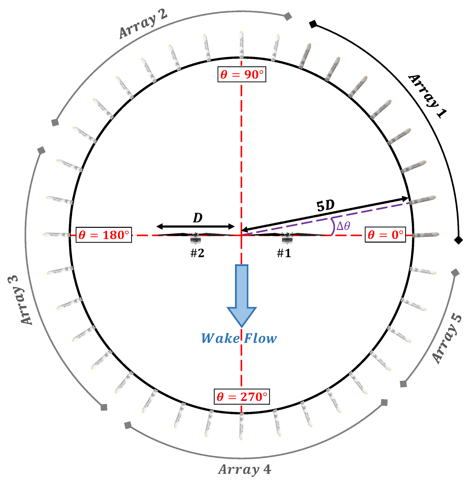
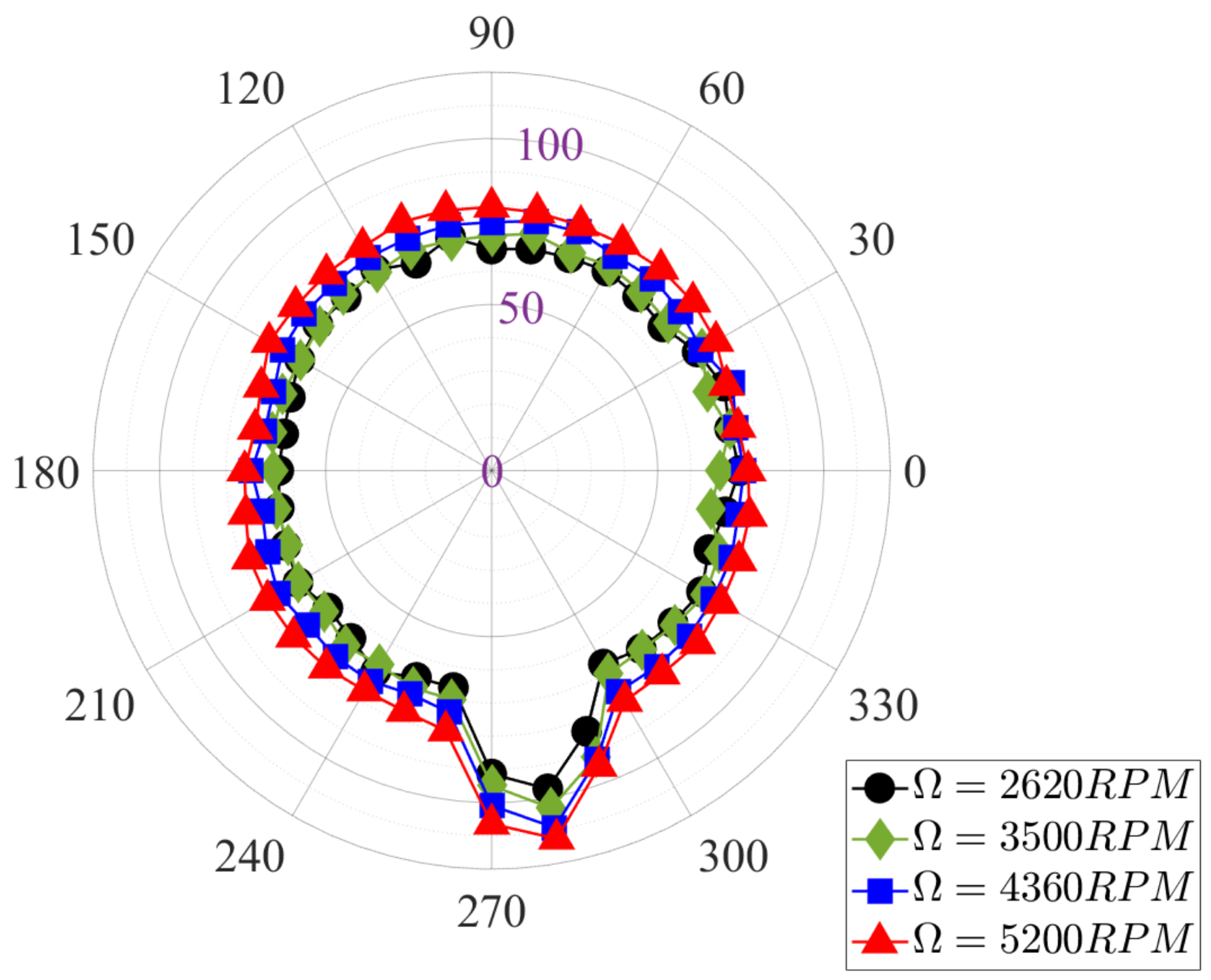
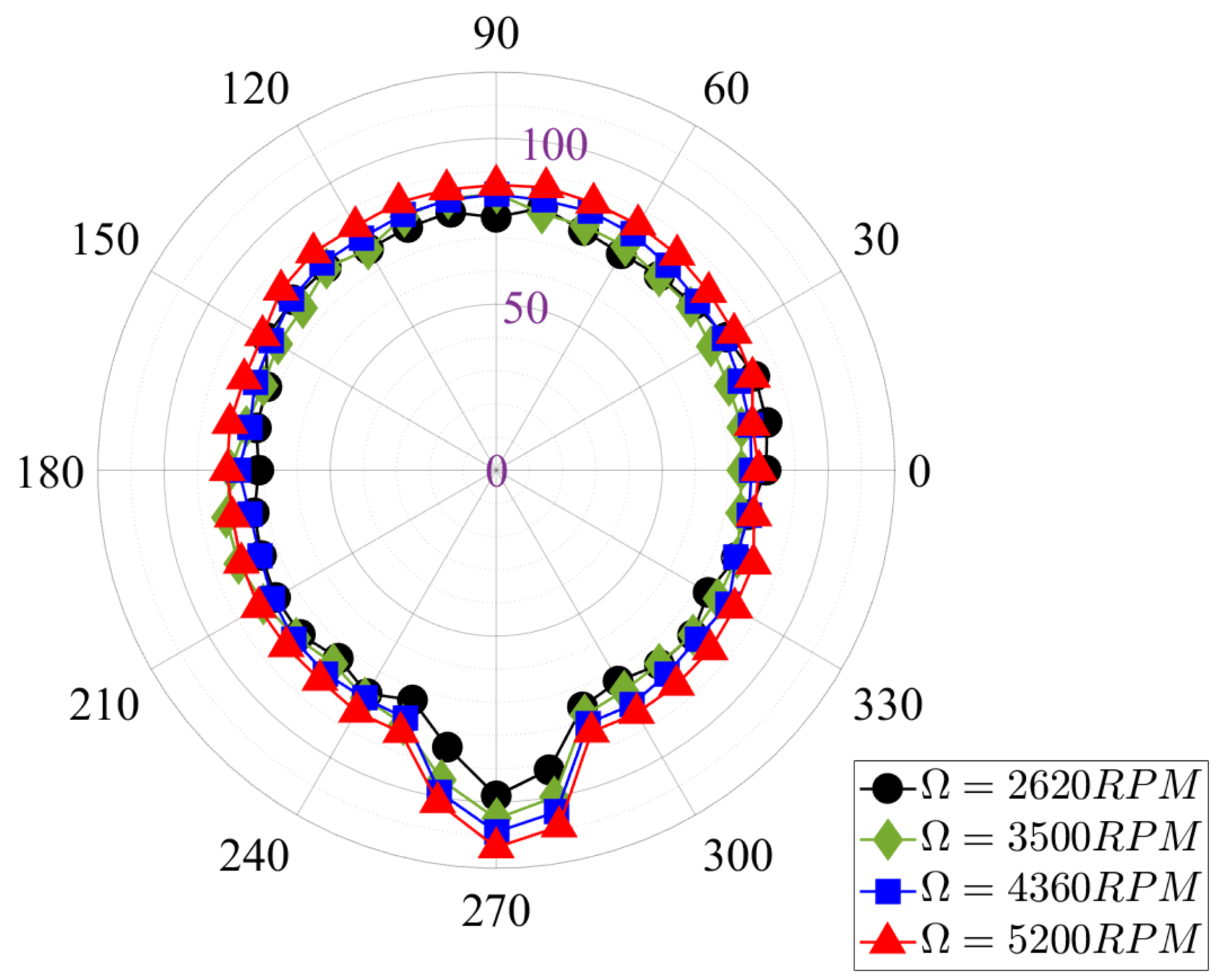
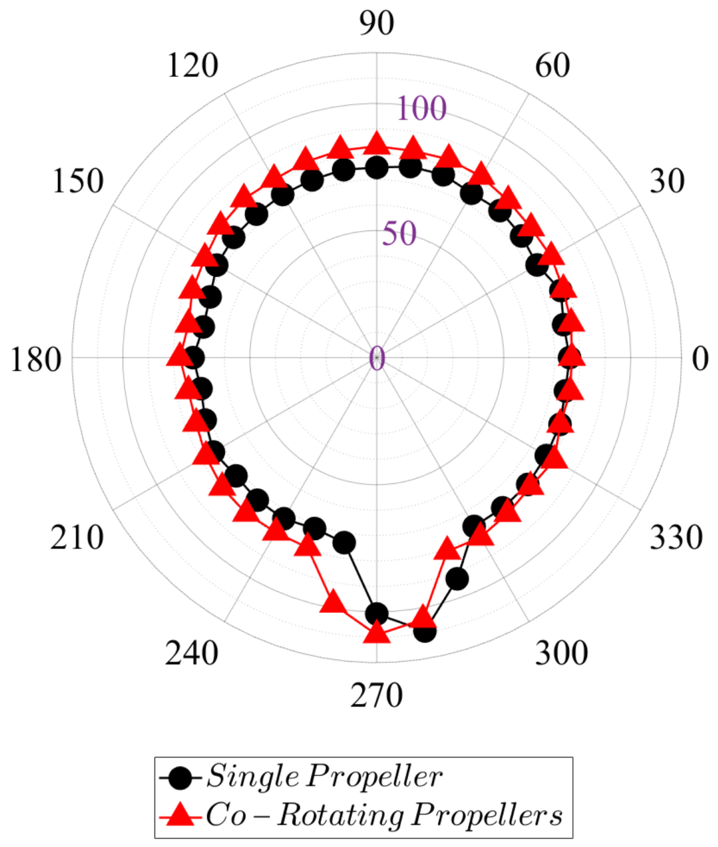
4.3. Aeroacoustic Characterization

To characterize the aeroacoustic behavior capturing the pressure fluctuations on the interaction between the rotors at the far field, the Over All Sound Pressure Level ($OASPL$) has been calculated and presented in the form of a directivity map. The $OASPL$ is defined as

$$OASPL=20{log}_{10}\left(\frac{p_{RMS}^{\prime }}{p_{ref}}\right),$$

(15)

where $p_{RMS}^{\prime }$ is the root mean square of the pressure fluctuation and $p_{ref}$ is the reference pressure equal to 20 $\mathsf{\mu }$ Pa (threshold of human hearing).

This physical quantity is representative of the entire energetic content of the pressure time series and, in this sense, can give us global information about the aeroacoustic behavior of the propellers.

To inspect the fundaments of the present aeroacoustic profile of the current experimental setup, a single rotor at the explored propeller speeds has been characterized as having a baseline reference. The results are shown in Figure 28, plotting the polar diagram of the OASPL. As expected, the sound source produced by the single rotor can be assumed to be a monopole. Furthermore, the wake impinges the microphone array at a far field in the region enclosed at ${250}^{\circ }\le \theta \le {300}^{\circ }$, at which a higher OASPL intensity is detected. In addition, the distribution reflects the asymmetry of the experimental setup established when one of the two rotors is off; hence, the polar diagram exhibits a bias on the right side of the vertical axis. The measurements were conducted by keeping propeller $\#2$ off and running only propeller $\#1$. The OASPL distributions are consistent with each other for all the explored rotor speeds, and the noise levels attain between ∼65 dB and ∼80 dB across the polar. Peaks in the range between 90 dB and 110 dB in the wake region are detected. The rotor speeds affect the intensities of the OASPL distributions, increasing consistently as the rotor speed augments. However, the noise source preserves its shape regardless of the rotor speeds.

As both the rotors run in a corotating propeller configuration, the polar plot becomes symmetric, as shown in Figure 29, reflecting the symmetry of the experimental setup. Consistently, the noise level increases as the rotor speed does. In addition, the region where the wakes impinge at the far field over the region enclosed at ${250}^{\circ }\le \theta \le {290}^{\circ }$ exhibits an intensified noise level. For instance, at $\mathrm{\Omega }=5200$ RPM, the OASPL value attains, on average, ∼85 dB; however, the maximum value peaks at 113 dB at $\theta ={270}^{\circ }$.

As expected, the noise level intensity captured for both corotating rotors is slightly higher than that detected for the single rotor configuration. This is more emphasized in the side and inflow regions.

For instance, Figure 30 shows the polar diagrams of the single rotor and side-by-side configurations as a comparison at $\mathrm{\Omega }=4360$ RPM. The noise increments from 2 dB for the two-rotor to that found for the single-rotor, despite the asymmetry of its OASPL distribution. There is a remarkable noise increment around the corotating propellers, resulting in a level of up to 10 dB, and the interaction noise weakens in correspondence with the wake flow. Spectral analysis has been performed by calculating the Sound Pressure Spectral Level (SPSL) to compare the finding of the most representative flow field structures and the sound profile of the corotating rotors.

The $SPSL$ is defined as

$$SPSL=10lo{g}_{10}\left(\frac{PSD\Delta f_{ref}}{p_{ref}^2}\right),$$

(16)

where $PSD$ stands for the Power Spectral Density of the pressure time series; $\Delta f_{ref}$ is the frequency resolution set equal to 1 Hz.

Finally, keeping in mind that the two measurement campaigns (fluid dynamics and acoustics) were not carried out simultaneously, a comparison between the two is reported. For the sake of brevity, a comparison plot between the power spectra of the time coefficients $a_1$ and $a_3$, representative of the wake-like motion and tip vortices, respectively, and the $SPSL$ at $\theta =0^{\circ }$, $\theta ={90}^{\circ }$, and $\theta ={180}^{\circ }$, at $\mathrm{\Omega }=5200$ RPM is depicted in Figure 31. A rather excellent match between the spectral peaks gathered from the POD analysis of the flow fields and the sound profile at the far field is found.

5. Conclusions

An investigation of the fluid-dynamic and aeroacoustic interactions of side-by-side rotors has been carried out at different rotating speeds by means of force, flow field, and microphonic measurements. The twin arrangement features a fixed configuration with a mutual distance between the propeller axes of 1.02 D. Four different rotating speeds, i.e., $2620,3500,4360$, and 5200 RPM, were explored.

The aerodynamic loads on each rotor in a side-by-side configuration exhibit a significant affection in terms of thrust and torque reductions in comparison to that found for a single propeller configuration. The interaction due to the propeller vicinity reduces the thrust in a range from $17.7\%$ down to $5.5\%$ as the rotating speed of both propellers increases. In addition, there is an increment in the level of aerodynamic load fluctuations, indicating a simultaneous flow interaction between the two established flow patterns. Similarly, the torque undergoes a reduction in intensity ranging from $30\%$ down to $9.5\%$, directly as the rotating speed increases.

The inspection of the spatial organization and the dynamic evolution of the flow structures through TR-PIV measurements at the axial plane figures out how the wakes interact with each other. The average velocity fields reveal that the flow interaction between the wakes generates recirculation regions within the plane at the periphery of the external shear layers. In the proximity of the rotor disks, the contraction of the wakes prevails over the interaction process, and the flow direction deflects toward the rotor axis of each propeller. Further downstream, the slipstream at the wakes interface promotes the interaction between them and, on average, smoothly merge into each other. Depending on the phase angle between the two rotors, this process can presumably produce a bias in the final flow direction. The merging of the wakes is reflected by the RMS of the velocity fluctuations, which present significant levels due to the travel of the tip vortices shed by each blade passage.

The modal analysis through the POD of the radial component of the velocity field sheds light on the spatial organization of large-scale structures. The distribution of the decomposed flow across the modes highlights that the first two modes, ${\phi }_1$ and ${\phi }_2$, phase shifted by $\pi /2$, represent a pair collecting most of the energy. This effect is more prominent at a lower rotating speed, 2620 RPM, which involves $44.5\%$ of the total energy. They describe the wave-like motion of the wakes, pulsating at $HBPF=1/3$, i.e., at the rotor speed. This behavior deviates from the results of a single rotor, which typically describes tip-blade vortical structures. Herein, these are encountered in pairs, phase shifted by $\pi /2$, of higher order modes. Even though the wake interaction affects the average flow field, the shedding of the vortices occurs mainly at $HBPF=1$, i.e., at the blade pass frequency. At $\mathrm{\Omega }=4360$ RPM, the phase shift angle between the rotors of $\gamma ={60}^{\circ }$ presumably affects the POD by capturing, at the third mode, a flapping motion of the wakes pulsating at $HBPF=1/3$. The wavelet analysis of the time coefficients confirms that the wakes maintain periodic behavior during the observation time, even in the presence of interaction effects.

The aeroacoustic investigation using a microphone array at a far field unveils the level of noise generated by either single or two propellers in corotating configurations at different rotating speeds. The single propeller exhibits a typical monopolar distribution, having the OASPL flattening between $65\mathrm{dB}$ and $80\mathrm{dB}$, except for the levels in the wake region rising between $90\mathrm{dB}$ and $110\mathrm{dB}$. On the other hand, the noise level increases with the rotating speed; the noise reaches the maximum of $113\mathrm{dB}$ at $\theta ={270}^{\circ }$, i.e., in correspondence with the wake region. In the side-by-side configuration, a higher level of noise was found, i.e., approximately $12\%$, particularly in the inlet flow and side zones (${180}^{\circ }\le \theta \le {220}^{\circ }$ and ${310}^{\circ }\le \theta \le {350}^{\circ }$). The spectral analysis of the noise reveals harmonic frequencies associated with the pulsation of coherent structures captured by the POD analysis.

References

1. Bouabdallah, S.; Becker, M.; Siegwart, R. Autonomous miniature flying robots: Coming soon!-research, development, and results. IEEE Robot. Autom. Mag. 2007, 14, 88–98. [Google Scholar] [CrossRef]
2. Shukla, D.; Hiremath, N.; Patel, S.; Komerath, N. Aerodynamic interactions study on low-Re coaxial and quad-rotor configurations. In Proceedings of the ASME International Mechanical Engineering Congress and Exposition, Tampa, FL, USA, 3–9 November 2017; American Society of Mechanical Engineers: New York, NY, USA, 2017; Volume 58424, p. V007T09A023. [Google Scholar] [CrossRef]
3. Tulwin, T. Low Reynolds Number Rotor Blade Aerodynamic Analysis. In MATEC Web of Conferences; EDP Sciences: Les Ulis, France, 2019; Volume 252, p. 04006. [Google Scholar] [CrossRef]
4. Sinibaldi, G.; Marino, L. Experimental analysis on the noise of propellers for small UAV. Appl. Acoust. 2013, 74, 79–88. [Google Scholar] [CrossRef]
5. Zhou, W.; Ning, Z.; Li, H.; Hu, H. An experimental investigation on rotor-to-rotor interactions of small UAV propellers. In Proceedings of the 35th AIAA Applied Aerodynamics Conference, Denver, CO, USA, 5–9 June 2017; p. 3744. [Google Scholar] [CrossRef]
6. Ko, J.; Kim, J.; Lee, S. Computational study of wake interaction and aeroacoustic characteristics in multirotor configurations. In INTER-NOISE and NOISE-CON Congress and Conference Proceedings; Institute of Noise Control Engineering: Reston, VA, USA, 2019; Volume 259, pp. 5145–5156. [Google Scholar]
7. Tinney, C.; Sirohi, J. Multirotor drone noise at static thrust. AIAA J. 2018, 56, 2816–2826. [Google Scholar] [CrossRef]
8. Shukla, D.; Komerath, N. Multirotor Drone Aerodynamic Interaction Investigation. Drones 2018, 2, 43. [Google Scholar] [CrossRef]
9. Stokkermans, T.; Usai, D.; Sinnige, T.; Veldhuis, L. Aerodynamic interaction effects between propellers in typical eVTOL vehicle configurations. J. Aircr. 2021, 58, 815–833. [Google Scholar] [CrossRef]
10. Zanotti, A.; Algarotti, D. Aerodynamic interaction between tandem overlapping propellers in eVTOL airplane mode flight condition. Aerosp. Sci. Technol. 2022, 124, 107518. [Google Scholar] [CrossRef]
11. Nargi, R.E.; De Gregorio, F.; Candeloro, P.; Ceglia, G.; Pagliaroli, T. Evolution of flow structures in twin-rotors wakes in drones by time-resolved PIV. J. Phys. Conf. Ser. 2021, 1977, 012008. [Google Scholar] [CrossRef]
12. Kim, H.D.; Perry, A.T.; Ansell, P.J. A review of distributed electric propulsion concepts for air vehicle technology. In Proceedings of the 2018 AIAA/IEEE Electric Aircraft Technologies Symposium (EATS), Cincinnati, OH, USA, 12–14 July 2018; pp. 1–21. [Google Scholar]
13. Zanotti, A. Experimental study of the aerodynamic interaction between side-by-side propellers in evtol airplane mode through stereoscopic particle image velocimetry. Aerospace 2021, 8, 239. [Google Scholar] [CrossRef]
14. Lumley, J.L. The structure of inhomogeneous turbulent flows. Atmos. Turbul. Radio Wave Propag. 1967, 166–178. [Google Scholar]
15. Andrianne, T.; Razak, N.; Dimitriadis, G.; Okamoto, S. Flow visualization and proper orthogonal decomposition of aeroelastic phenomena. In Wind Tunnels; BoD: Paris, France, 2011; pp. 87–104. [Google Scholar] [CrossRef]
16. Pagliaroli, T.; Camussi, R. Wall pressure fluctuations in rectangular partial enclosures. J. Sound Vib. 2015, 341, 116–137. [Google Scholar] [CrossRef]
17. Pagliaroli, T.; Gambioli, F.; Saltari, F.; Cooper, J. Proper orthogonal decomposition, dynamic mode decomposition, wavelet and cross wavelet analysis of a sloshing flow. J. Fluids Struct. 2022, 112, 103603. [Google Scholar] [CrossRef]
18. Berkooz, G.; Holmes, P.; Lumley, J. The proper orthogonal decomposition in the analysis of turbulent flows. Annu. Rev. Fluid Mech. 1993, 25, 539–575. [Google Scholar] [CrossRef]
19. Magionesi, F.; Dubbioso, G.; Muscari, R.; Di Mascio, A. Modal analysis of the wake past a marine propeller. J. Fluid Mech. 2018, 855, 469–502. [Google Scholar] [CrossRef]
20. Sirovich, L. Turbulence and the dynamics of coherent structures. III. Dynamics and scaling. Q. Appl. Math. 1987, 45, 583–590. [Google Scholar] [CrossRef]
21. Meyer, K.; Pedersen, J.; Özcan, O. A turbulent jet in crossflow analysed with proper orthogonal decomposition. J. Fluid Mech. 2007, 583, 199–227. [Google Scholar] [CrossRef]
22. Mallat, S. A theory for multiresolution signal decomposition: The wavelet representation. IEEE Trans. Pattern Anal. Mach. Intell. 1989, 11, 674–693. [Google Scholar] [CrossRef]
23. Daubechies, I. Ten Lectures on Wavelets; SIAM: Philadelphia, PA, USA, 1992. [Google Scholar]
24. Lau, K.M.; Weng, H. Climate signal detection using wavelet transform: How to make a time series sing. Bull. Am. Math. Soc. 1995, 76, 2391–2402. [Google Scholar] [CrossRef]
25. Mancinelli, M.; Pagliaroli, T.; Marco, A.D.; Camussi, R.; Castelain, T. Wavelet decomposition of hydrodynamic and acoustic pressures in the near field of the jet. J. Sound Vib. 2017, 813, 716–749. [Google Scholar] [CrossRef]
26. Pagliaroli, T.; Mancinelli, M.; Troiani, G.; Iemma, U.; Camussi, R. Fourier and wavelet analyses of intermittent and resonant pressure components in a slot burner. J. Sound Vib. 2018, 413, 205–224. [Google Scholar] [CrossRef]
27. Tsai, R. A versatile camera calibration technique for high-accuracy 3D machine vision metrology using off-the-shelf TV cameras and lenses. IEEE J. Robot. Autom. 1987, 3, 323–344. [Google Scholar] [CrossRef]
28. Westerweel, J.; Dabiri, D.; Gharib, M. The effect of a discrete window offset on the accuracy of cross-correlation analysis of digital PIV recordings. Exp. Fluids 1997, 23, 20–28. [Google Scholar] [CrossRef]
29. Wereley, S.T.; Meinhart, C. Second-order accurate particle image velocimetry. Exp. Fluids 2001, 31, 258–268. [Google Scholar] [CrossRef]
30. Willert, C.E.; Gharib, M. Digital particle image velocimetry. Exp. Fluids 1991, 10, 181–193. [Google Scholar] [CrossRef]
31. Raffel, M.; Willert, C.; Wereley, S.; Kompenhans, J. Particle Image Velocimetry—A Practical Guide; Springer: Berlin/Heidelberg, Germany; New York, NY, USA, 2007. [Google Scholar] [CrossRef]
32. Chen, M.; Cranes, D.; Hubner, J. Experimental investigation of rotor-wing interaction at low disk loading and low Reynolds number. In Proceedings of the AIAA Aviation 2019 Forum, Dallas, TX, USA, 17–21 June 2019; p. 3034. [Google Scholar] [CrossRef]
33. Leishman, J.G.; Baker, A.; Coyne, A. Measurements of rotor tip vortices using three-component laser Doppler velocimetry. J. Am. Helicopter Soc. 1996, 41, 342–353. [Google Scholar] [CrossRef]
34. Li, H.; Burggraf, O.; Conlisk, A. Formation of a rotor tip vortex. J. Aircr. 2002, 39, 739–749. [Google Scholar] [CrossRef]
35. Nargi, R.E.; De Gregorio, F.; Camussi, R. Four blades rotor model aerodynamic characterization and experimental investigation of rotor wake and sling load interaction. J. Phys. Conf. Ser. 2018, 1110, 012012. [Google Scholar] [CrossRef]
36. De Gregorio, F.; Visingardi, A.; Nargi, R. Investigation of a helicopter model rotor wake interacting with a cylindrical sling load. In Proceedings of the 44th European Rotorcraft Forum, Delft, The Netherlands, 18–21 September 2018. [Google Scholar]
37. De Gregorio, F.; Visingardi, A. Vortex detection criteria assessment for PIV data in rotorcraft applications. Exp. Fluids 2020, 61, 1–22. [Google Scholar] [CrossRef]
38. Graftieaux, L.; Michard, M.; Grosjean, N. Combining PIV, POD and vortex identification algorithms for the study of unsteady turbulent swirling flows. Meas. Sci. Technol. 2001, 12, 1422. [Google Scholar] [CrossRef]
39. Ning, Z.; Hu, H. An Experimental Study on the Aerodynamics and Aeroacoustic Characteristics of Small Propellers. In Proceedings of the 54th AIAA Aerospace Sciences Meeting, San Diego, CA, USA, 4–8 January 2016; p. 1785. [Google Scholar] [CrossRef]
40. Weightman, J.L.; Amili, O.; Honnery, D.; Soria, J.; Edgington-Mitchell, D. Signatures of shear-layer unsteadiness in proper orthogonal decomposition. Exp. Fluids 2018, 59, 180. [Google Scholar] [CrossRef]
41. Yang, Y.; Sciacchitano, A.; Veldhuis, L.; Eitelberg, G. Spatial-temporal and modal analysis of propeller induced ground vortices by particle image velocimetry. Phys. Fluids 2016, 28, 105103. [Google Scholar] [CrossRef]
42. Al-Khazali, H.A.; Askari, M.R. Geometrical and graphical representations analysis of lissajous figures in rotor dynamic system. IOSR J. Eng. 2012, 2, 971–978. [Google Scholar] [CrossRef]
Figure 1. Blade characteristics: radial distribution of chord c / R (red line), thickness T h k / c (blue dash-dot line), and blade pitch β (green dashed line) (left); isometric view of the blade and airfoils highlighted by colors (right).
Aerospace 10 00851 g001
Figure 2. Rotor rig interfaced with 6-component balance.
Aerospace 10 00851 g002
Figure 3. The TR-PIV experimental setup.
Aerospace 10 00851 g003
Figure 4. Front view of the rotor rig and measurement regions with reference frame (a); top view of the rotor rig with the propellers’ clearances from the supports (b).
Aerospace 10 00851 g004
Figure 5. Rotor rig and microphone array mounted in the semianechoic chamber.
Aerospace 10 00851 g005
Figure 6. Sketch of the experimental setup within the semianechoic chamber of CIRA.
Aerospace 10 00851 g006
Figure 7. Comparison between the isolated propeller and the side-by-side configuration. Thrust (a) and torque (b) vs. rotational speed for the case of a single rotor (square red markers) and side-by-side configuration (delta blue markers). The 2nd-order polynomial fitting lines are plotted: a solid red line for the single propeller data and a dashed blue line for the tandem configuration. In both plots, the error bars represent the standard deviation.
Aerospace 10 00851 g007
Figure 8. Effect on thrust (solid red line) and torque (dashed blue line) due to the interaction of the two rotors.
Aerospace 10 00851 g008
Figure 9. Isocontours with stream traces of the time-average flow field color-coded with the dimensionless velocity magnitude | U ¯ | / U t i p at Ω = 2620 RPM (a), 3500 RPM (b), 4360 RPM (c), and 5200 RPM (d).
Aerospace 10 00851 g009
Figure 10. Definition of phase angle γ .
Aerospace 10 00851 g010
Figure 11. Isocontours of the velocity fluctuations color-coded with the magnitude of their normalized RMS, | V R M S | / U t i p , at Ω = 2620 RPM (a), 3500 RPM (b), 4360 RPM (c), and 5200 RPM (d).
Aerospace 10 00851 g011
Figure 12. Region of Interest (ROI) for the POD analysis superimposed at isocontours of the time-average flow field color-coded with the dimensionless velocity magnitude | U ¯ | / U t i p at Ω = 2620 RPM.
Aerospace 10 00851 g012
Figure 13. Energy distribution in percentage across the first eight modes for Ω = 2620 RPM (a), 3500 RPM (b), 4360 RPM (c), and 5200 RPM (d).
Aerospace 10 00851 g013
Figure 14. First four POD modes describing the wave-like motion of the interacting wakes, φ 1 (a) and φ 2 (b), and the tip vortices, φ 3 (c) and φ 4 (d), at Ω = 2620 RPM. Positive (red) and negative (blue) isosurface.
Aerospace 10 00851 g014
Figure 15. Power spectra of the first four-time coefficients, a 1 (solid blue), a 2 (dashed red), a 3 (solid green), and a 4 (dashed magenta), at Ω = 2620 RPM.
Aerospace 10 00851 g015
Figure 16. Scatter plots of the first four-time coefficients at Ω = 2620 R P M compared for different combinations: a 1 a 2 (a), a 2 a 3 (b), a 1 a 3 (c), and a 3 a 4 (d).
Aerospace 10 00851 g016
Figure 17. Isocontours of the wavelet power spectra of time coefficients a 1 (a), a 2 (b), a 3 (c), and a 4 (d) at Ω = 2620 RPM.
Aerospace 10 00851 g017
Figure 18. Scatter plots of the first four-time coefficients at Ω = 3500 R P M compared for different combinations: a 1 a 2 (a), a 2 a 3 (b), a 1 a 3 (c), and a 3 a 4 (d).
Aerospace 10 00851 g018
Figure 19. Isocontours of the wavelet power spectra of time coefficients a 1 (a), a 2 (b), a 3 (c), and a 4 (d) at Ω = 3500 RPM.
Aerospace 10 00851 g019
Figure 20. First six POD modes describing the wave-like motion of the interacting wakes, φ 1 (a) and φ 2 (b), the flapping motion φ 3 (c), and the tip vortices, φ 4 (d), φ 5 (e), and φ 6 (f), at Ω = 4360 RPM. Positive (red) and negative (blue) isosurface.
Aerospace 10 00851 g020
Figure 21. Power spectra of the first six-time coefficients: a 1 (solid blue), a 2 (dashed red), a 3 (dotted black), a 4 (solid green), a 5 (dashed magenta), and a 6 (dashed cyan) at Ω = 4360 RPM.
Aerospace 10 00851 g021
Figure 22. Scatter plots of the first six-time coefficients at Ω = 4360 R P M compared for different combinations: a 1 a 2 (a), a 1 a 3 (b), a 4 a 5 (c), and a 5 a 6 (d).
Aerospace 10 00851 g022
Figure 23. Isocontours of the wavelet power spectra of time coefficients a 1 (a), a 2 (b), a 3 (c), a 4 (d), a 5 (e), and a 6 (f) at Ω = 4360 RPM.
Aerospace 10 00851 g023
Figure 24. First six POD modes describing the wave-like motion of the interacting wakes, φ 1 (a) and φ 2 (b), and the tip vortices, φ 3 (c), φ 4 (d), φ 5 (e), and φ 6 (f), at Ω = 5200 RPM. Positive (red) and negative (blue) isosurface.
Aerospace 10 00851 g024
Figure 25. Power spectra of the first six-time coefficients: a 1 (solid blue), a 2 (dashed red), a 3 (solid green), a 4 (dashed magenta), a 5 (solid black), and a 6 (dashed cyan) at Ω = 5200 RPM.
Aerospace 10 00851 g025
Figure 26. Scatter plots of the first six-time coefficients at Ω = 5200 R P M compared for different combinations: a 1 a 2 (a), a 2 a 3 (b), a 3 a 4 (c), and a 5 a 6 (d).
Aerospace 10 00851 g026
Figure 27. Isocontours of the wavelet power spectra of time coefficients: a 1 (a), a 2 (b), a 3 (c), a 4 (d), a 5 (e), and a 6 (f) at Ω = 5200 RPM.
Aerospace 10 00851 g027
Figure 28. Polar diagram of the OASPL at the explored rotor speeds for the single rotor configuration.
Aerospace 10 00851 g028
Figure 29. Corotating propeller configuration: polar diagram of the OASPL at distance of d = 1.02 D for all rotational regimes.
Aerospace 10 00851 g029
Figure 30. Polar diagram of the OASPL: comparison between single propeller configuration (black circle) and corotating propeller configuration (red triangle) at Ω = 4360 RPM.
Aerospace 10 00851 g030
Figure 31. Comparison plot of the power spectra of the time coefficients a 1 and a 3 (solid blue and dashed green line, respectively) and S P S L at θ = 0 , θ = 90 , and θ = 180 (red, black, and purple line, respectively) at Ω = 5200 RPM.
Aerospace 10 00851 g031