Distributed Robust Formation Tracking Control for Quadrotor UAVs with Unknown Parameters and Uncertain Disturbances

Abstract

In this paper, the distributed formation tracking control problem of quadrotor unmanned aerial vehicles is considered. Adaptive backstepping inherently accommodates model uncertainties and external disturbances, making it a robust choice for the dynamic and unpredictable environments in which unmanned aerial vehicles operate. This paper designs a formation flight control scheme for quadrotor unmanned aerial vehicles based on adaptive backstepping technology. The proposed control scheme is divided into two parts. For the position subsystem, a distributed robust formation tracking control scheme is developed to achieve formation flight of quadrotor unmanned aerial vehicles and track the desired flight trajectory. For the attitude subsystem, an adaptive disturbance rejection control scheme is proposed to achieve attitude stabilization during unmanned aerial vehicle flight under uncertain disturbances. Compared to existing results, the novelty of this paper lies in presenting a disturbance rejection flight control scheme for actual quadrotor unmanned aerial vehicle formations, without the need to know the model parameters of each unmanned aerial vehicle. Finally, a quadrotor unmanned aerial vehicle swarm system is used to verify the effectiveness of the proposed control scheme.

1. Introduction

In recent years, the cooperative control of quadrotor unmanned aerial vehicles (UAVs) has garnered considerable attention due to its broad applications in fields such as wireless communication, nuclear radiation detection, and agricultural mapping. Formation control is a pivotal research area within the domain of cooperative control for quadrotor UAVs. For example, Liu and Li [1] explored formation control for UAVs in precision agriculture, emphasizing its potential to optimize aerial coverage and reduce operational costs. Meanwhile, Liu et al. [2] illustrated the importance of formation control in urban surveillance applications, showcasing its effectiveness in wide-area monitoring with minimal energy expenditure.

A formation comprising multiple low-cost UAVs can supplant an expensive multi-functional UAV in completing intricate tasks. Moreover, UAV formations offer system redundancy and reconfiguration capabilities [3]. Formation control of quadrotor UAVs has drawn significant research interest, given its potential applications in both military and civilian sectors [4,5,6]. From the perspective of control mechanisms, the existing methodologies for quadrotor UAV formation control encompass the leader-follower method [7], artificial potential method [8], behavior-based method [9], etc. Recent work in [10] delved into dynamic formation collision avoidance control for quadrotor UAVs, employing the virtual structure method. In [11], a consensus-based approach was utilized to craft a time-varying formation tracking control scheme for quadrotor UAVs. However, the quadrotor UAV models considered in the aforementioned literature tend to be simplified, and the designed formation control schemes rely on the model parameters of the quadrotor UAV. In many practical applications of quadrotor UAVs, obtaining accurate model parameters can be challenging. Recently, many flight control methods that do not rely on quadrotor model parameters have been proposed. For example, in [12], a quadrotor UAV dynamics modeling method using feedforward neural networks was introduced. This method served as the predictive model for precise position control in a model predictive controller. In [13], the application of model predictive contouring control addressed the optimal flight trajectory problem for quadrotors with multiple waypoints. In a multifunctional quadrotor UAV formation, the model parameters of individual UAVs might differ. Therefore, designing a flight control scheme for the quadrotor UAV formation that does not rely on system model parameters is crucial. This is the first research motivation of this paper.

In addition, quadrotor UAVs are highly sensitive to uncertain disturbances, making it essential to design effective disturbance rejection flight control schemes for them. Extensive research on disturbance rejection control for individual UAVs has been conducted in existing literature. For quadrotor UAV swarms, uncertain disturbances acting on each UAV will affect neighboring UAVs through the communication network. Hence, designing disturbance rejection control schemes for quadrotor UAV swarms is a more complex task. Existing literature has also conducted research on the disturbance rejection control problem for quadrotor UAV formations [14,15,16,17]. For example, in [14], a formation active disturbance rejection control method based on inner and outer loops was proposed. In [15], the time-varying rendezvous problem of UAV swarms with a master-slave consistency hierarchy was discussed, and a fully distributed formation disturbance rejection control scheme was presented. Note that in both [14,15], the quadrotor UAVs were simplified into a basic linear second-order model for study, which limits the practicality of the proposed methods. For the unsimplified quadrotor UAV model, existing literature has not yet effectively designed a disturbance suppression control scheme for its formation. This is the second research motivation of this paper.

In this paper, a distributed robust formation tracking control method is proposed for quadrotor UAVs with unknown parameters and uncertain disturbances. The proposed method has the following novelties. First, a more practical formation tracking control method is proposed in this paper, which does not need to use the model parameters of the quadrotor UAV. Second, an adaptive disturbance rejection control scheme for quadrotor UAV swarms is developed. In the presence of uncertain disturbances, this scheme can still achieve formation tracking control for quadrotor UAV swarms, and the tracking error can eventually converge to zero.

The structure of this paper is arranged in the following manner. In Section 2 and Section 3, a distributed formation tracking control scheme and an adaptive disturbance rejection attitude control method are designed for quadrotor UAVs. The efficacy of the proposed control method is validated in Section 4. Finally, Section 5 concludes the paper.

2. Distributed Robust Formation Tracking Control for Quadrotor UAVs

In this section, a distributed formation flight control method is developed for quadrotor UAVs to achieve the following three control objectives: (1) form the desired formation; (2) track the desired flight trajectory; (3) reduce the influence of uncertain disturbances.

2.1. Graph Theory

The communication topology among a group of N quadrotor UAVs is considered as an undirected graph $\mathrm{G}=(\mathbb{W},\mathbb{S})$, where $\mathbb{W}\triangleq \{1,2,\cdots ,N\}$ denotes the vertex set and $\mathbb{S}\triangleq \{(i,j):i\in \mathbb{W},j\in {\mathcal{N}}_i\}$ denotes the edge set. The neighbor set of the ith UAV is ${\mathcal{N}}_i\triangleq \{j\in \mathbb{W}$: there is a communication link between UAV i and UAV j, $j\ne i\}$. Define a weight ${\mathbf{a}}_{ij}$ for each edge $(i,j)\in \mathbb{S}$, ${\mathbf{a}}_{ij}=1$ if $j\in {\mathcal{N}}_i$, and ${\mathbf{a}}_{ij}=0$ otherwise. The Laplacian matrix is $\mathcal{L}=[{\mathbf{w}}_{ij}]\in {\mathbb{R}}^{N\times N}$, where ${\mathbf{w}}_{ii}={\sum }_{j=1,j\ne i}^N{\mathbf{a}}_{ij}$ and ${\mathbf{w}}_{ij}=-{\mathbf{a}}_{ij}$$(j\ne i)$. The leader adjacency matrix is $\mathcal{D}=diag\{{\mathbf{d}}_1,\cdots ,{\mathbf{d}}_N\}$, where ${\mathbf{d}}_i>0$ if UAV i can obtain the desired flight trajectory and ${\mathbf{d}}_i=0$ otherwise. An undirected graph is considered connected if there is a path between every pair of distinct vertices.

Next, two useful lemmas are introduced.

Lemma 1.

[18]. If the undirected graph $\mathrm{G}$ is connected, and at least one UAV can obtain the desired flight trajectory, then the symmetric matrix $\mathcal{L}+\mathcal{D}$ is positive definite.

Lemma 2.

[19]. For any positive constant κ and any scalar function $\varsigma \in \mathbb{R}$, the following inequality holds.

$$\begin{array}{c}\hfill 0\le |\varsigma |-\frac{{\varsigma }^2}{\sqrt{{\varsigma }^2+{\kappa }^2}}\le \kappa .\end{array}$$

Remark 1.

Lemmas 1 and 2 are often used in existing literature. Specifically, a detailed proof of Lemma 2 can be found in [19]. In this paper, Lemma 2 will play a crucial role in the subsequent controller design process.

2.2. Quadrotor UAV Position Dynamic Model

In this paper, define $\mathcal{E}={[\varphi ,\theta ,\phi ]}^T$ as the attitude of the quadrotor UAV, where $\varphi ,$ $\theta$ and $\phi$ denote the angles of roll, pitch and yaw, respectively. As described in [20], the rotation matrix that describes the transformation from the body-fixed frame to the earth-fixed frame is denoted as

$$R_t=\left[\begin{array}{ccc}{C}_{\phi }{C}_{\theta }& C_{\phi }{S}_{\varphi }{S}_{\theta }-S_{\phi }{C}_{\varphi }& C_{\phi }{C}_{\varphi }{S}_{\theta }+S_{\phi }{S}_{\varphi }\\ S_{\phi }{C}_{\theta }& S_{\phi }{S}_{\varphi }{S}_{\theta }+C_{\phi }{C}_{\varphi }& S_{\phi }{C}_{\varphi }{S}_{\theta }-C_{\phi }{S}_{\varphi }\\ -S_{\theta }& S_{\varphi }{C}_{\theta }& C_{\varphi }{C}_{\theta }\end{array}\right]$$

(1)

where $S_{(·)}$ and $C_{(·)}$ denote sin$(·)$ and cos$(·)$, respectively.

Define $h={[x,y,z]}^T$ as the position of the quadrotor UAV. As described in [20], the translational dynamic equations are given as

$$\begin{array}{c}\hfill \left[\begin{array}{c}\ddot{x}\\ \ddot{y}\\ \ddot{z}\end{array}\right]=R_t\left[\begin{array}{c}0\\ 0\\ U_s\end{array}\right]+\left[\begin{array}{c}0\\ 0\\ -g\end{array}\right]-\frac{1}{m}\left[\begin{array}{c}{d}_x\dot{x}\\ d_y\dot{y}\\ d_z\dot{z}\end{array}\right]\end{array}$$

(2)

where m is the quadrotor mass; $d_x$, $d_y$, $d_z$ are the air drag coefficients; $U_s=b({\Omega }_1^2+{\Omega }_2^2+{\Omega }_3^2+{\Omega }_4^2)/m$, b is the lift coefficient and ${\Omega }_k$$(k=1,2,3,4)$ are the rotor speed; g is the acceleration of gravity.

In this paper, the formation tracking control problem of quadrotor UAVs is studied. From (2), the position dynamic system of the ith $(i=1,\cdots ,N)$ UAV can be described as

$$\begin{array}{c}\hfill \left\{\begin{array}{c}{\dot{h}}_{i,l}=v_{i,l}+w_{h_{i,l}}\hfill \\ {\dot{v}}_{i,l}=u_{i,l}+{\Theta }_{i,l}{v}_{i,l}+w_{v_{i,l}},l=1,2,3\hfill \end{array}\right.\end{array}$$

(3)

where $[h_{i,1},h_{i,2},h_{i,3}]=[x_i,y_i,z_i]$ and $[v_{i,1},v_{i,2},v_{i,3}]=[{\dot{x}}_i,{\dot{y}}_i,{\dot{z}}_i]$ are the position and velocity of UAV i, respectively; $[{\Theta }_{i,1},{\Theta }_{i,2},{\Theta }_{i,3}]=[-\frac{d_x}{m},-\frac{d_y}{m},-\frac{d_z}{m}]$ are the unknown system parameters; $u_{i,1},u_{i,2},u_{i,3}$ are the control inputs, and $u_{i,1}=(C_{{\varphi }_i}{S}_{{\theta }_i}{C}_{{\phi }_i}+S_{{\varphi }_i}{S}_{{\phi }_i})U_{s_i},$ $u_{i,2}=(C_{{\varphi }_i}{S}_{{\theta }_i}{S}_{{\phi }_i}-S_{{\varphi }_i}{C}_{{\phi }_i})U_{s_i},$ $u_{i,3}=C_{{\varphi }_i}{C}_{{\theta }_i}{U}_{s_i}-g.$ In addition, $w_{h_{i,l}}$ and $w_{v_{i,l}}$ represent uncertain disturbances.

Assumption 1.

The uncertain disturbances satisfy

$$\begin{array}{c}\hfill |w_{h_{i,l}}|\le {\overline{w}}_h,|w_{v_{i,l}}|\le {\overline{w}}_v,i=1,\cdots ,N\end{array}$$

(4)

where ${\overline{w}}_h>0$ and ${\overline{w}}_v>0$ are unknown constants.

Definition 1.

A time-varying formation formed by a group of N UAVs is specified by $\mathbf{F}(t)={[{\mathbf{F}}_1^T(t),\cdots ,{\mathbf{F}}_N^T(t)]}^T\in {\mathbb{R}}^{3N}$, where ${\mathbf{F}}_i(t)={[{\mathbf{F}}_{i,1},{\mathbf{F}}_{i,2},{\mathbf{F}}_{i,3}]}^T\in {\mathbb{R}}^3$ is the piecewise continuously formation vector. Formation tracking control of quadrotor UAVs can be achieved if

$$\begin{array}{c}\hfill \underset{t\to +\infty }{lim}[h_i(t)-{\mathbf{F}}_i(t)-\mathbf{n}(t)]=0,i=1,\cdots ,N\end{array}$$

(5)

where $h_i(t)={[x_i,y_i,z_i]}^T$; and $\mathbf{n}(t)={[{\mathbf{n}}_1,{\mathbf{n}}_2,{\mathbf{n}}_3]}^T$ represents the desired flight trajectory.

Assumption 2.

The desired flight trajectory satisfies

$$\begin{array}{c}\hfill |{\mathbf{n}}_l|\le \overline{\mathbf{n}},l=1,2,3\end{array}$$

(6)

where $\overline{\mathbf{n}}>0$ is an unknown constant.

Remark 2.

Note that ${\mathbf{F}}_i(t)$ represents the position of each UAV in the formation. When all ${\mathbf{F}}_i(t)=0$, Equation (5) becomes ${lim}_{t\to +\infty }[h_i(t)-\mathbf{n}(t)]=0$, indicating that all UAVs eventually achieve a consistent state. Therefore, the definition of UAV formation tracking control in this paper encompasses the consensus tracking control problems in most of the existing literature.

Control objective: This paper achieves the following control objectives: (1) forming a desired quadrotor UAV formation; (2) tracking the desired flight trajectory; (3) reducing the influence of disturbances. The control block diagram of the quadrotor UAV is shown in Figure 1.

2.3. Distributed Formation Tracking Controller Design

For the ith UAV, define two error variables

$${\chi }_{i,l}={\displaystyle \sum _{j=1}^N}{\mathbf{a}}_{ij}(h_{i,l}-{\mathbf{F}}_{i,l}-h_{j,l}+{\mathbf{F}}_{j,l})+{\mathbf{d}}_i(h_{i,l}-{\mathbf{F}}_{i,l}-{\mathbf{n}}_l)$$

(7)

$${\eta }_{i,l}=v_{i,l}-{\alpha }_{i,l},l=1,2,3$$

(8)

where ${\alpha }_{i,l}$ are the virtual control functions. The detailed design procedure is given as follows:

Step 1: By defining ${\chi }_l={[{\chi }_{1,l},\cdots ,{\chi }_{N,l}]}^T$, one can obtain ${\chi }_l=(\mathcal{L}+\mathcal{D})e_l$, where $e_l={\underline{h}}_l-{\underline{\mathbf{F}}}_l-{\underline{\mathbf{n}}}_l$ with ${\underline{h}}_l={[h_{1,l},\cdots ,h_{N,l}]}^T$, ${\underline{\mathbf{F}}}_l={[{\mathbf{F}}_{1,l},\cdots ,{\mathbf{F}}_{N,l}]}^T$, and ${\underline{\mathbf{n}}}_l={[{\mathbf{n}}_l,\cdots ,{\mathbf{n}}_l]}^T$. Then, the derivative of $e_l$ satisfies

$$\begin{array}{c}\hfill {\dot{e}}_l=\left[\begin{array}{c}{\alpha }_{1,l}+{\eta }_{1,l}+w_{h_{1,l}}-{\dot{\mathbf{F}}}_{1,l}-{\dot{\mathbf{n}}}_l\\ ⋮\\ {\alpha }_{N,l}+{\eta }_{N,l}+w_{h_{N,l}}-{\dot{\mathbf{F}}}_{N,l}-{\dot{\mathbf{n}}}_l\end{array}\right].\end{array}$$

(9)

The virtual control function ${\alpha }_{i,l}$ is chosen as

$$\begin{array}{c}\hfill \begin{array}{c}{\alpha }_{i,l}=-k_{h_{i,l}}{\chi }_{i,l}+{\dot{\mathbf{F}}}_{i,l}+{\mathbf{d}}_i{\dot{\mathbf{n}}}_l-\frac{{\chi }_{i,l}}{\sqrt{{\chi }_{i,l}^2+{\delta }_{i,l}^2}}{\widehat{\mu }}_{h_{i,l}}\hfill \end{array}\end{array}$$

(10)

where $k_{h_{i,l}}>0$ is a design constant; ${\widehat{\mu }}_{h_{i,l}}$ is the estimate of ${\mu }_{h_{i,l}}={\overline{w}}_h+(1-{\mathbf{d}}_i)\overline{\mathbf{n}}$; and ${\delta }_{i,l}(t)$ is a positive continuous function satisfying ${lim}_{t\to \infty }{\int }_{t_0}^t{\delta }_{i,l}(\tau )d\tau \le {\overline{\delta }}_{i,l}<+\infty$, and ${\overline{\delta }}_{i,l}$ is a positive constant. This function ensures asymptotic stability for the system in question, which is pivotal for the safe operation of UAVs.

Consider the Lyapunov function

$$\begin{array}{c}\hfill \begin{array}{c}{V}_{h_l}=\frac{1}{2}{e}_l^T(\mathcal{L}+\mathcal{D})e_l+{\displaystyle \sum _{i=1}^N}\frac{1}{2{\lambda }_{h_{i,l}}}{\tilde{\mu }}_{h_{i,l}}^2\hfill \end{array}\end{array}$$

(11)

where the estimation error ${\tilde{\mu }}_{h_{i,l}}={\mu }_{h_{i,l}}-{\widehat{\mu }}_{h_{i,l}}$; and ${\lambda }_{h_{i,l}}>0$ is a design parameter. From Lemma 1 we know that the Lyapunov function (11) is positive definite.

From (9)–(11), the derivative of $V_{h_l}$ satisfies

$$\begin{array}{c}\hfill \begin{array}{c}{\dot{V}}_{h_l}\le {\displaystyle \sum _{i=1}^N}[-k_{h_{i,l}}{\chi }_{i,l}^2+(|{\chi }_{i,l}|-\frac{{\chi }_{i,l}^2}{\sqrt{{\chi }_{i,l}^2+{\delta }_{i,l}^2}}){\mu }_{h_{i,l}}\hfill \\ +{\chi }_{i,l}{\eta }_{i,l}+\frac{1}{{\lambda }_{h_{i,l}}}{\tilde{\mu }}_{h_{i,l}}(\frac{{\lambda }_{h_{i,l}}{\chi }_{i,l}^2}{\sqrt{{\chi }_{i,l}^2+{\delta }_{i,l}^2}}-{\dot{\widehat{\mu }}}_{h_{i,l}})].\hfill \end{array}\end{array}$$

(12)

The parameter update law is chosen as

$$\begin{array}{c}\hfill \begin{array}{c}{\dot{\widehat{\mu }}}_{h_{i,l}}=\frac{{\lambda }_{h_{i,l}}{\chi }_{i,l}^2}{\sqrt{{\chi }_{i,l}^2+{\delta }_{i,l}^2}}.\hfill \end{array}\end{array}$$

(13)

Then, by applying Lemma 2, we have

$$\begin{array}{c}\hfill \begin{array}{c}{\dot{V}}_{h_l}\le {\displaystyle \sum _{i=1}^N}(-k_{h_{i,l}}{\chi }_{i,l}^2+{\chi }_{i,l}{\eta }_{i,l}+{\delta }_{i,l}{\mu }_{h_{i,l}}).\hfill \end{array}\end{array}$$

(14)

Step 2: Note that ${\alpha }_{i,l}$ is a function of $h_{i,l}$, ${\delta }_{i,l}$, ${\widehat{\mu }}_{h_{i,l}}$, ${\mathbf{n}}_l$, ${\dot{\mathbf{n}}}_l$, and $h_{j,l}$. From (3) and (10), the derivative of ${\eta }_{i,l}$ satisfies

$$\begin{array}{c}\hfill \begin{array}{c}{\dot{\eta }}_{i,l}={\dot{v}}_{i,l}-{\dot{\alpha }}_{i,l}\hfill \\ =u_{i,l}+{\Theta }_{i,l}{v}_{i,l}+w_{v_{i,l}}-{\dot{\alpha }}_{i,l}\hfill \\ =u_{i,l}+{\Theta }_{i,l}{v}_{i,l}+w_{v_{i,l}}-\frac{\partial {\alpha }_{i,l}}{\partial h_{i,l}}(v_{i,l}+w_{h_{i,l}})-\frac{\partial {\alpha }_{i,l}}{\partial {\delta }_{i,l}}{\dot{\delta }}_{i,l}-\frac{\partial {\alpha }_{i,l}}{\partial {\widehat{\mu }}_{h_{i,l}}}{\dot{\widehat{\mu }}}_{h_{i,l}}\hfill \\ -{\mathbf{d}}_i\frac{\partial {\alpha }_{i,l}}{\partial {\mathbf{n}}_l}{\dot{\mathbf{n}}}_l-{\mathbf{d}}_i\frac{\partial {\alpha }_{i,l}}{\partial {\dot{\mathbf{n}}}_l}{\ddot{\mathbf{n}}}_l-{\displaystyle \sum _{j=1}^N}{\mathbf{a}}_{ij}\frac{\partial {\alpha }_{i,l}}{\partial h_{j,l}}(v_{j,l}+w_{h_{j,l}}).\hfill \end{array}\end{array}$$

(15)

The formation flight controller is designed as

$$\begin{array}{c}\hfill \begin{array}{c}{u}_{i,l}=-k_{v_{i,l}}{\eta }_{i,l}-{\widehat{\Theta }}_{i,l}{v}_{i,l}+\frac{\partial {\alpha }_{i,l}}{\partial h_{i,l}}{v}_{i,l}+\frac{\partial {\alpha }_{i,l}}{\partial {\delta }_{i,l}}{\dot{\delta }}_{i,l}+\frac{\partial {\alpha }_{i,l}}{\partial {\widehat{\mu }}_{h_{i,l}}}{\dot{\widehat{\mu }}}_{h_{i,l}}+{\mathbf{d}}_i\frac{\partial {\alpha }_{i,l}}{\partial {\mathbf{n}}_l}{\dot{\mathbf{n}}}_l\hfill \\ +{\mathbf{d}}_i\frac{\partial {\alpha }_{i,l}}{\partial {\dot{\mathbf{n}}}_l}{\ddot{\mathbf{n}}}_l+{\displaystyle \sum _{j=1}^N}{\mathbf{a}}_{ij}\frac{\partial {\alpha }_{i,l}}{\partial h_{j,l}}{v}_{j,l}-\frac{{\eta }_{i,l}{\varpi }_{i,l}^2}{\sqrt{{\eta }_{i,l}^2{\varpi }_{i,l}^2+{\delta }_{i,l}^2}}{\widehat{\mu }}_{v_{i,l}}-{\chi }_{i,l}\hfill \end{array}\end{array}$$

(16)

where $k_{v_{i,l}}>0$ is a design constant; ${\varpi }_{i,l}=\sqrt{1+{(\frac{\partial {\alpha }_{i,l}}{\partial h_{i,l}})}^2+{\sum }_{j=1}^N{\mathbf{a}}_{ij}{(\frac{\partial {\alpha }_{i,l}}{\partial h_{j,l}})}^2}$; and ${\widehat{\mu }}_{v_{i,l}}$ is the estimate of ${\mu }_{v_{i,l}}=max\{{\overline{w}}_h,{\overline{w}}_v,\overline{\mathbf{n}}\}$.

Construct the following Lyapunov function

$$\begin{array}{c}\hfill \begin{array}{c}{V}_{v_l}=V_{h_l}+\frac{1}{2}{\displaystyle \sum _{i=1}^N}({\eta }_{i,l}^2+\frac{1}{{\lambda }_{h_{i,l}}}{\tilde{\mu }}_{v_{i,l}}^2+\frac{1}{{\lambda }_{{\Theta }_{i,l}}}{\tilde{\Theta }}_{i,l}^2)\hfill \end{array}\end{array}$$

(17)

where the estimation errors ${\tilde{\mu }}_{v_{i,l}}={\mu }_{v_{i,l}}-{\widehat{\mu }}_{v_{i,l}}$ and ${\tilde{\Theta }}_{i,l}={\Theta }_{i,l}-{\widehat{\Theta }}_{i,l}$; ${\lambda }_{v_{i,l}}>0$ and ${\lambda }_{{\Theta }_{i,l}}>0$ are design parameters. We know that the Lyapunov function (17) is positive definite.

From (14)–(17), the derivative of $V_{v_l}$ satisfies

$$\begin{array}{c}\hfill \begin{array}{c}{\dot{V}}_{v_l}\le {\displaystyle \sum _{i=1}^N}(-k_{h_{i,l}}{\chi }_{i,l}^2+{\delta }_{i,l}{\mu }_{h_{i,l}})+{\displaystyle \sum _{i=1}^N}{\eta }_{i,l}(-k_{v_{i,l}}{\eta }_{i,l}+w_{v_{i,l}}-\frac{\partial {\alpha }_{i,l}}{\partial h_{i,l}}{w}_{h_{i,l}}\hfill \\ -{\displaystyle \sum _{j=1}^N}{\mathbf{a}}_{ij}\frac{\partial {\alpha }_{i,l}}{\partial h_{j,l}}{w}_{h_{j,l}}+{\tilde{\Theta }}_{i,l}{v}_{i,l}-\frac{{\eta }_{i,l}{\varpi }_{i,l}^2}{\sqrt{{\eta }_{i,l}^2{\varpi }_{i,l}^2+{\delta }_{i,l}^2}}{\widehat{\mu }}_{v_{i,l}})-{\displaystyle \sum _{i=1}^N}(\frac{1}{{\lambda }_{h_{i,l}}}{\tilde{\mu }}_{v_{i,l}}{\dot{\widehat{\mu }}}_{v_{i,l}}\hfill \\ +\frac{1}{{\lambda }_{{\Theta }_{i,l}}}{\tilde{\Theta }}_{i,l}{\dot{\widehat{\Theta }}}_{i,l})\hfill \\ \le {\displaystyle \sum _{i=1}^N}[-k_{h_{i,l}}{\chi }_{i,l}^2+(|{\eta }_{i,l}|{\varpi }_{i,l}-\frac{{\eta }_{i,l}^2{\varpi }_{i,l}^2}{\sqrt{{\eta }_{i,l}^2{\varpi }_{i,l}^2+{\delta }_{i,l}^2}}){\mu }_{v_{i,l}}-k_{v_{i,l}}{\eta }_{i,l}^2+{\delta }_{i,l}{\mu }_{h_{i,l}}\hfill \\ +\frac{1}{{\lambda }_{v_{i,l}}}{\tilde{\mu }}_{v_{i,l}}(\frac{{\lambda }_{v_{i,l}}{\eta }_{i,l}^2{\varpi }_{i,l}^2}{\sqrt{{\eta }_{i,l}^2{\varpi }_{i,l}^2+{\delta }_{i,l}^2}}-{\dot{\widehat{\mu }}}_{v_{i,l}})+\frac{1}{{\lambda }_{{\Theta }_{i,l}}}{\tilde{\Theta }}_{i,l}({\lambda }_{{\Theta }_{i,l}}{v}_{i,l}{\eta }_{i,l}-{\dot{\widehat{\Theta }}}_{i,l})].\hfill \end{array}\end{array}$$

(18)

The adaptive update laws are chosen as

$$\begin{array}{c}\hfill \begin{array}{c}{\dot{\widehat{\mu }}}_{v_{i,l}}=\frac{{\lambda }_{v_{i,l}}{\eta }_{i,l}^2{\varpi }_{i,l}^2}{\sqrt{{\eta }_{i,l}^2{\varpi }_{i,l}^2+{\delta }_{i,l}^2}},{\dot{\widehat{\Theta }}}_{i,l}={\lambda }_{{\Theta }_{i,l}}{v}_{i,l}{\eta }_{i,l}.\hfill \end{array}\end{array}$$

(19)

Then, by applying Lemma 2, we have

$$\begin{array}{c}\hfill \begin{array}{c}{\dot{V}}_{v_l}\le {\displaystyle \sum _{i=1}^N}(-k_{h_{i,l}}{\chi }_{i,l}^2-k_{v_{i,l}}{\eta }_{i,l}^2+{\delta }_{i,l}{\mu }_{h_{i,l}}+{\delta }_{i,l}{\mu }_{v_{i,l}}).\hfill \end{array}\end{array}$$

(20)

Now, we present the analysis results.

Theorem 1.

Consider the quadrotor UAV swarm system (3), the formation tracking controller (16), and the adaptive laws (13) and (19). All the signals in the closed-loop system are globally bounded, and the quadrotor UAV swarm can achieve time-varying formation flying and track the virtual leader.

Proof. 

Integrating both sizes of (20), it follows that

$$\begin{array}{c}\hfill \begin{array}{c}{V}_{v_l}(t)+k_{h_{i,l}}{\int }_0^t{\chi }_{i,l}^2(\tau )d\tau +k_{v_{i,l}}{\int }_0^t{\eta }_{i,l}^2(\tau )d\tau \hfill \\ \le V_{v_l}(0)+({\mu }_{h_{i,l}}+{\mu }_{v_{i,l}}){\overline{\delta }}_{i,l}.\hfill \end{array}\end{array}$$

(21)

From the definition of $V_{v_l}$ in (17), one can get that ${\chi }_{i,l}$, ${\eta }_{i,l}$, ${\widehat{\mu }}_{h_{i,l}}$, ${\widehat{\mu }}_{v_{i,l}}$, and ${\widehat{\Theta }}_{i,l}$$(l=1,2,3)$ are bounded. From (10), (16), and Lemma 1, ${\alpha }_{i,l}$, $u_{i,l}$, and $h_{i,l}$ are bounded. Therefore, the boundedness of all the signals is guaranteed, and ${\dot{\chi }}_{i,l}$ is bounded. By applying Barbalat’s lemma, one has ${lim}_{t\to \infty }{\chi }_{i,l}(t)=0$. From the definition of ${\chi }_{i,l}$ and Lemma 1, it follows that formation tracking control of quadrotor UAVs can be achieved, i.e., ${lim}_{t\to +\infty }[h_i(t)-{\mathbf{F}}_i(t)-\mathbf{n}(t)]=0$. This completes the proof. □

Remark 3.

When the distributed formation tracking controller $u_{i,1},u_{i,2},u_{i,3}$ is designed, and the desired yaw angle ${\phi }_{i,0}$ is treated as an additional reference signal, then the desired roll angle ${\varphi }_{i,0}$, the desired pitch angle ${\theta }_{i,0}$, and the control input $U_{s_i}$ can be obtained in the following way

$$\begin{array}{c}\hfill \left\{\begin{array}{c}{\theta }_{i,0}=arctan(\frac{C_{{\phi }_{i,0}}{u}_{i,1}+S_{{\phi }_{i,0}}{u}_{i,2}}{u_{i,3}+g})\hfill \\ {\varphi }_{i,0}=arctan(\frac{(S_{{\phi }_{i,0}}{u}_{i,1}-C_{{\phi }_{i,0}}{u}_{i,2})C_{{\theta }_{i,0}}}{u_{i,3}+g})\hfill \\ U_{s_i}=\sqrt{u_{i,1}^2+u_{i,2}^2+{(u_{i,3}+g)}^2}.\hfill \end{array}\right.\end{array}$$

(22)

Since $u_{i,1},u_{i,2},u_{i,3}$, and ${\phi }_{i,0}$ are continuous and bounded, it is known that ${\theta }_{i,0},{\varphi }_{i,0}$ and $U_{s_i}$ are bounded.

3. Disturbance Rejection Control of Quadrotor UAV Attitude

In this section, an adaptive disturbance rejection attitude control method will be designed for the quadrotor UAV. The angular velocity with respect to the attitude is given as $\mathcal{W}={[p,q,r]}^T$. As described in [21], The correlation between the attitude angle and angular velocity can be denoted by

$$\left(\begin{array}{c}\dot{\varphi }\\ \dot{\theta }\\ \dot{\phi }\end{array}\right)=\left[\begin{array}{ccc}1& T_{\theta }{S}_{\varphi }& T_{\theta }{C}_{\varphi }\\ 0& C_{\varphi }& -S_{\varphi }\\ 0& S_{\varphi }/C_{\theta }& C_{\varphi }/C_{\theta }\end{array}\right]\left(\begin{array}{c}p\\ q\\ r\end{array}\right)$$

(23)

where $T_{(·)}$ denotes tan$(·)$.

By employing the Newton-Euler formulation, the rotational dynamic equations can be derived as

$$J_b\dot{\mathcal{W}}=-\mathcal{W}\times J_b\mathcal{W}-M_g-M_d+M_b$$

(24)

$$M_g={\displaystyle \sum _{i=1}^4}{J}_r(\mathcal{W}\times e_3){(-1)}^{i+1}{\Omega }_i$$

(25)

$$M_d=diag\{d_{\varphi },d_{\theta },d_{\phi }\}\dot{\mathcal{E}}$$

(26)

$$M_b=\left[\begin{array}{c}lb({\Omega }_4^2-{\Omega }_2^2)\\ lb({\Omega }_3^2-{\Omega }_1^2)\\ \sigma ({\Omega }_1^2-{\Omega }_2^2+{\Omega }_3^2-{\Omega }_4^2)\end{array}\right]$$

(27)

where $J_b=diag\{J_x,J_y,J_z\}$; $M_g$ is the resultant torque; $M_d$ is the aerodynamic frictions torque; $M_b$ is the rotor torque; l is the distance between rotor and center of mass; $\sigma$ denotes the reverse moment coefficient; $J_r$ is the rotational inertia of each rotor; $J_x$, $J_y$, $J_z$ are the rotary inertia; and $d_{\varphi },d_{\theta },d_{\phi }$ are the drag coefficients.

Then, the following dynamic equations can be derived

$$\begin{array}{c}\hfill \left\{\begin{array}{c}\dot{p}={\tau }_{1}qr-{\tau }_2\mathcal{O}q-{\tau }_{3}p+U_p\hfill \\ \dot{q}={\tau }_{4}pr+{\tau }_5\mathcal{O}p-{\tau }_{6}q+U_q\hfill \\ \dot{r}={\tau }_{7}pq-{\tau }_{8}r+U_r\hfill \end{array}\right.\end{array}$$

(28)

where

• ${\tau }_1=\frac{J_y-J_z}{J_x},{\tau }_2=\frac{J_r}{J_x},{\tau }_3=\frac{d_{\varphi }}{J_x},{\tau }_4=\frac{J_z-J_x}{J_y},$
• ${\tau }_5=\frac{J_r}{J_y},{\tau }_6=\frac{d_{\theta }}{J_y},{\tau }_7=\frac{J_x-J_y}{J_z},{\tau }_8=\frac{d_{\phi }}{J_z},$
• $\mathcal{O}={\Omega }_1-{\Omega }_2+{\Omega }_3-{\Omega }_4,U_p=lb({\Omega }_4^2-{\Omega }_2^2)/J_x,$
• $U_q=lb({\Omega }_3^2-{\Omega }_1^2)/J_y,U_r=\sigma ({\Omega }_1^2-{\Omega }_2^2+{\Omega }_3^2-{\Omega }_4^2)/J_z.$

Consider a group of N quadrotor UAVs, define $m_{i,1}={\varphi }_i$, $m_{i,2}={\theta }_i$, $m_{i,3}={\phi }_i$, $n_{i,1}=p_i$, $n_{i,2}=q_i$, and $n_{i,3}=r_i$, then the following unified attitude system can be obtained

$$\begin{array}{c}\hfill \left\{\begin{array}{c}{\dot{m}}_{i,l}=n_{i,l}+f_{i,l}+w_{m_{i,l}}\hfill \\ {\dot{n}}_{i,l}=U_{n_{i,l}}+{\Phi }_{i,l}^T{\xi }_{i,l}(n_i)+w_{n_{i,l}},l=1,2,3\hfill \end{array}\right.\end{array}$$

(29)

where $w_{m_{i,l}}$ and $w_{n_{i,l}}$ represent uncertain disturbances, and

• $f_{i,1}=T_{m_{i,2}}{S}_{m_{i,1}}{n}_{i,2}+T_{m_{i,2}}{C}_{m_{i,1}}{n}_{i,3},$
• $f_{i,2}=C_{m_{i,1}}{n}_{i,2}-S_{m_{i,1}}{n}_{i,3}-n_{i,2},$
• $f_{i,3}=S_{m_{i,1}}/C_{m_{i,2}}{n}_{i,2}+C_{m_{i,1}}/C_{m_{i,2}}{n}_{i,3}-n_{i,3},$
• ${\xi }_{i,1}(n_i)={[n_{i,2}{n}_{i,3},-{\mathcal{O}}_i{n}_{i,2},-n_{i,1}]}^T,$
• ${\xi }_{i,2}(n_i)={[n_{i,1}{n}_{i,3},{\mathcal{O}}_i{n}_{i,1},-n_{i,2}]}^T,$
• ${\xi }_{i,3}(n_i)={[n_{i,1}{n}_{i,2},-n_{i,3}]}^T,{\Phi }_{i,1}={[{\tau }_1,{\tau }_2,{\tau }_3]}^T,$
• ${\Phi }_{i,2}={[{\tau }_4,{\tau }_5,{\tau }_6]}^T,{\Phi }_{i,3}={[{\tau }_7,{\tau }_8]}^T.$

Assumption 3.

The uncertain disturbances satisfy

$$\begin{array}{c}\hfill |w_{m_{i,l}}|\le {\overline{w}}_m,|w_{n_{i,l}}|\le {\overline{w}}_n\end{array}$$

(30)

where ${\overline{w}}_m>0$ and ${\overline{w}}_n>0$ are positive constants.

Remark 4.

Note that each UAV has to estimate the desired yaw angle ${\phi }_0$ by the information obtained from its neighbors. Inspired by [22], design the following distributed estimator

$$\begin{array}{c}\hfill \begin{array}{c}{\dot{\phi }}_{i,0}=-{ϵ}_1[{\displaystyle \sum _{j=1}^N}{\mathbf{a}}_{ij}({\phi }_{i,0}-{\phi }_{j,0})+{\mathbf{d}}_i({\phi }_{i,0}-{\phi }_0)]\hfill \\ -{ϵ}_2\mathrm{sgn}[{\displaystyle \sum _{j=1}^N}{\mathbf{a}}_{ij}({\phi }_{i,0}-{\phi }_{j,0})+{\mathbf{d}}_i({\phi }_{i,0}-{\phi }_0)]\hfill \end{array}\end{array}$$

(31)

where ${\phi }_{i,0}$ is an estimate of ${\phi }_0$; ${ϵ}_1>0$ and ${ϵ}_2>0$ are design parameters; $\mathrm{sgn}$ is the signum function. From Theorem 3.1 in [22], one can get that ${\phi }_{i,0}\to {\phi }_0$ in finite time.

For the ith UAV, define two error variables

$$\begin{array}{c}\hfill \begin{array}{c}{\epsilon }_{i,l}=m_{i,l}-{\vartheta }_{i,l},{\rho }_{i,l}=n_{i,l}-{\beta }_{i,l},l=1,2,3\hfill \end{array}\end{array}$$

(32)

where ${\vartheta }_{i,1}={\varphi }_{i,0}$, ${\vartheta }_{i,2}={\theta }_{i,0}$, and ${\vartheta }_{i,3}={\phi }_{i,0}$; and ${\beta }_{i,l}$ are the virtual control functions. From (22) and (31), there exists an unknown constant $\overline{\vartheta }>0$ such that $|{\dot{\vartheta }}_{i,l}|\le \overline{\vartheta }$. The detailed design procedure is given as follows:

Step 1: The derivative of ${\epsilon }_{i,l}$ satisfies

$$\begin{array}{c}\hfill \begin{array}{c}{\dot{\epsilon }}_{i,l}=n_{i,l}+f_{i,l}+w_{m_{i,l}}-{\dot{\vartheta }}_{i,l}.\hfill \end{array}\end{array}$$

(33)

The virtual control function ${\beta }_{i,l}$ is chosen as

$$\begin{array}{c}\hfill \begin{array}{c}{\beta }_{i,l}=-k_{m_{i,l}}{\epsilon }_{i,l}-f_{i,l}-\frac{{\epsilon }_{i,l}}{\sqrt{{\epsilon }_{i,l}^2+{\delta }_{i,l}^2}}{\widehat{\mu }}_{m_{i,l}}\hfill \end{array}\end{array}$$

(34)

where $k_{m_{i,l}}>0$ is a design constant; ${\widehat{\mu }}_{m_{i,l}}$ is the estimate of ${\mu }_{m_{i,l}}={\overline{w}}_m+\overline{\vartheta }$. Consider the Lyapunov function

$$\begin{array}{c}\hfill \begin{array}{c}{V}_{m_{i,l}}=\frac{1}{2}{\epsilon }_{i,l}^2+\frac{1}{2{\lambda }_{m_{i,l}}}{\tilde{\mu }}_{m_{i,l}}^2\hfill \end{array}\end{array}$$

(35)

where the estimation errors ${\tilde{\mu }}_{m_{i,l}}={\mu }_{m_{i,l}}-{\widehat{\mu }}_{m_{i,l}}$; and ${\lambda }_{m_{i,l}}>0$ is a design parameter. We know that the Lyapunov function (35) is positive definite.

From (33)–(35), the derivative of $V_{m_{i,l}}$ satisfies

$$\begin{array}{c}\hfill \begin{array}{c}{\dot{V}}_{m_{i,l}}\le -k_{m_{i,l}}{\epsilon }_{i,l}^2+(|{\epsilon }_{i,l}|-\frac{{\epsilon }_{i,l}^2}{\sqrt{{\epsilon }_{i,l}^2+{\delta }_{i,l}^2}}){\mu }_{m_{i,l}}\hfill \\ +{\epsilon }_{i,l}{\rho }_{i,l}+\frac{1}{{\lambda }_{m_{i,l}}}{\tilde{\mu }}_{m_{i,l}}(\frac{{\lambda }_{m_{i,l}}{\epsilon }_{i,l}^2}{\sqrt{{\epsilon }_{i,l}^2+{\delta }_{i,l}^2}}-{\dot{\widehat{\mu }}}_{m_{i,l}}).\hfill \end{array}\end{array}$$

(36)

The parameter update law is chosen as

$$\begin{array}{c}\hfill \begin{array}{c}{\dot{\widehat{\mu }}}_{m_{i,l}}=\frac{{\lambda }_{m_{i,l}}{\epsilon }_{i,l}^2}{\sqrt{{\epsilon }_{i,l}^2+{\delta }_{i,l}^2}}.\hfill \end{array}\end{array}$$

(37)

Then, by applying Lemma 2, we have

$$\begin{array}{c}\hfill \begin{array}{c}{\dot{V}}_{h_l}\le -k_{m_{i,l}}{\epsilon }_{i,l}^2+{\epsilon }_{i,l}{\rho }_{i,l}+{\delta }_{i,l}{\mu }_{m_{i,l}}.\hfill \end{array}\end{array}$$

(38)

Step 2: From (29) and (32), the derivative of ${\rho }_{i,l}$ satisfies

$$\begin{array}{c}\hfill \begin{array}{c}{\dot{\rho }}_{i,l}={\dot{n}}_{i,l}-{\dot{\beta }}_{i,l}\hfill \\ =U_{n_{i,l}}+{\Phi }_{i,l}^T{\xi }_{i,l}(n_i)+w_{n_{i,l}}-\frac{\partial {\beta }_{i,l}}{\partial {\delta }_{i,l}}{\dot{\delta }}_{i,l}-\frac{\partial {\beta }_{i,l}}{\partial {\widehat{\mu }}_{m_{i,l}}}{\dot{\widehat{\mu }}}_{m_{i,l}}-\frac{\partial {\beta }_{i,l}}{\partial m_{i,l}}{\dot{m}}_{i,l}\hfill \\ =U_{n_{i,l}}+{\Phi }_{i,l}^T{\xi }_{i,l}(n_i)+w_{n_{i,l}}-\frac{\partial {\beta }_{i,l}}{\partial {\delta }_{i,l}}{\dot{\delta }}_{i,l}-\frac{\partial {\beta }_{i,l}}{\partial {\widehat{\mu }}_{m_{i,l}}}{\dot{\widehat{\mu }}}_{m_{i,l}}-\frac{\partial {\beta }_{i,l}}{\partial m_{i,l}}(n_{i,l}\hfill \\ +f_{i,l}+w_{m_{i,l}}).\hfill \end{array}\end{array}$$

(39)

The attitude controller is designed as

$$\begin{array}{c}\hfill \begin{array}{c}{U}_{n_{i,l}}=-k_{n_{i,l}}{\rho }_{i,l}-{\epsilon }_{i,l}-{\widehat{\Phi }}_{i,l}^T{\xi }_{i,l}(n_i)+\frac{\partial {\beta }_{i,l}}{\partial {\widehat{\mu }}_{m_{i,l}}}{\dot{\widehat{\mu }}}_{m_{i,l}}\hfill \\ +\frac{\partial {\beta }_{i,l}}{\partial {\delta }_{i,l}}{\dot{\delta }}_{i,l}+\frac{\partial {\beta }_{i,l}}{\partial m_{i,l}}(n_{i,l}+f_{i,l})-\frac{{\rho }_{i,l}{\psi }_{i,l}^2}{\sqrt{{\rho }_{i,l}^2{\psi }_{i,l}^2+{\delta }_{i,l}^2}}{\widehat{\mu }}_{n_{i,l}}.\hfill \end{array}\end{array}$$

(40)

where $k_{n_{i,l}}>0$ is a design constant; ${\widehat{\mu }}_{n_{i,l}}$ is the estimate of ${\mu }_{n_{i,l}}=max\{{\overline{w}}_m,{\overline{w}}_n,\overline{\vartheta }\}$; and ${\psi }_{i,l}=\sqrt{1+{(\frac{\partial {\beta }_{i,l}}{\partial m_{i,l}})}^2}.$

Construct the following Lyapunov function

$$\begin{array}{c}\hfill \begin{array}{c}{V}_{n_{i,l}}=V_{m_{i,l}}+\frac{1}{2}({\rho }_{i,l}^2+\frac{1}{{\lambda }_{n_{i,l}}}{\tilde{\mu }}_{n_{i,l}}^2+\frac{1}{{\lambda }_{{\Phi }_{i,l}}}{\tilde{\Phi }}_{i,l}^T{\tilde{\Phi }}_{i,l})\hfill \end{array}\end{array}$$

(41)

where the estimation errors ${\tilde{\mu }}_{n_{i,l}}={\mu }_{n_{i,l}}-{\widehat{\mu }}_{n_{i,l}}$ and ${\tilde{\Phi }}_{i,l}={\Phi }_{i,l}-{\widehat{\Phi }}_{i,l}$; ${\lambda }_{n_{i,l}}>0$ and ${\lambda }_{{\Phi }_{i,l}}>0$ are design parameters. We know that the Lyapunov function (41) is positive definite.

From (38)–(41), the derivative of $V_{n_{i,l}}$ satisfies

$$\begin{array}{c}\hfill \begin{array}{c}{\dot{V}}_{n_{i,l}}\le -k_{m_{i,l}}{\epsilon }_{i,l}^2+{\delta }_{i,l}{\mu }_{m_{i,l}}+{\rho }_{i,l}(-k_{n_{i,l}}{\rho }_{i,l}+{\tilde{\Phi }}_{i,l}^T{\xi }_{i,l}(n_i)+w_{n_{i,l}}\hfill \\ -\frac{\partial {\beta }_{i,l}}{\partial m_{i,l}}{w}_{m_{i,l}}-\frac{{\rho }_{i,l}{\psi }_{i,l}^2}{\sqrt{{\rho }_{i,l}^2{\psi }_{i,l}^2+{\delta }_{i,l}^2}}{\widehat{\mu }}_{n_{i,l}})-\frac{1}{{\lambda }_{n_{i,l}}}{\tilde{\mu }}_{n_{i,l}}{\dot{\widehat{\mu }}}_{n_{i,l}}-\frac{1}{{\lambda }_{{\Phi }_{i,l}}}{\tilde{\Phi }}_{i,l}^T{\dot{\widehat{\Phi }}}_{i,l}\hfill \\ \le -k_{m_{i,l}}{\epsilon }_{i,l}^2+(|{\rho }_{i,l}|{\psi }_{i,l}-\frac{{\rho }_{i,l}^2{\psi }_{i,l}^2}{\sqrt{{\rho }_{i,l}^2{\psi }_{i,l}^2+{\delta }_{i,l}^2}}){\mu }_{n_{i,l}}+\frac{1}{{\lambda }_{n_{i,l}}}{\tilde{\mu }}_{n_{i,l}}(\frac{{\lambda }_{n_{i,l}}{\rho }_{i,l}^2{\psi }_{i,l}^2}{\sqrt{{\rho }_{i,l}^2{\psi }_{i,l}^2+{\delta }_{i,l}^2}}-{\dot{\widehat{\mu }}}_{n_{i,l}})\hfill \\ -k_{n_{i,l}}{\rho }_{i,l}^2+\frac{1}{{\lambda }_{{\Phi }_{i,l}}}{\tilde{\Phi }}_{i,l}^T({\lambda }_{{\Phi }_{i,l}}{\rho }_{i,l}{\xi }_{i,l}(n_i)-{\dot{\widehat{\Phi }}}_{i,l})+{\delta }_{i,l}{\mu }_{m_{i,l}}.\hfill \end{array}\end{array}$$

(42)

The parameter update laws are chosen as

$$\begin{array}{c}\hfill \begin{array}{c}{\dot{\widehat{\mu }}}_{n_{i,l}}=\frac{{\lambda }_{n_{i,l}}{\rho }_{i,l}^2{\psi }_{i,l}^2}{\sqrt{{\rho }_{i,l}^2{\psi }_{i,l}^2+{\delta }_{i,l}^2}},{\dot{\widehat{\Phi }}}_{i,l}={\lambda }_{{\Phi }_{i,l}}{\rho }_{i,l}{\xi }_{i,l}(n_i).\hfill \end{array}\end{array}$$

(43)

Then, by applying Lemma 2, we have

$$\begin{array}{c}\hfill \begin{array}{c}{\dot{V}}_{n_{i,l}}\le -k_{m_{i,l}}{\epsilon }_{i,l}^2-k_{n_{i,l}}{\rho }_{i,l}^2+{\delta }_{i,l}{\mu }_{m_{i,l}}+{\delta }_{i,l}{\mu }_{n_{i,l}}.\hfill \end{array}\end{array}$$

(44)

Now, we present the analysis results.

Theorem 2.

Consider the quadrotor UAV attitude system (29), the attitude controller (40), and the adaptive laws (37) and (43). All the signals in the closed-loop system are globally bounded, and the tracking error of the attitude angle system can converge to zero.

Proof. 

Integrating both sizes of (44), it follows that

$$\begin{array}{c}\hfill \begin{array}{c}{V}_{n_{i,l}}(t)+k_{m_{i,l}}{\int }_0^t{\epsilon }_{i,l}^2(\tau )d\tau +k_{n_{i,l}}{\int }_0^t{\rho }_{i,l}^2(\tau )d\tau \hfill \\ \le V_{n_{i,l}}(0)+({\mu }_{m_{i,l}}+{\mu }_{n_{i,l}}){\overline{\delta }}_{i,l}.\hfill \end{array}\end{array}$$

(45)

From the definition of $V_{n_{i,l}}$, one can get that ${\epsilon }_{i,l}$, ${\rho }_{i,l}$, ${\widehat{\mu }}_{m_{i,l}}$, ${\widehat{\mu }}_{n_{i,l}}$, and ${\widehat{\Phi }}_{i,l}$$(l=1,2,3)$ are bounded. From (32), (33), and (40), $m_{i,l}$, $n_{i,l}$, ${\beta }_{i,l}$ and $U_{n_{i,l}}$ are bounded. Therefore, the boundedness of all the signals is guaranteed, and ${\dot{\epsilon }}_{i,l}$ is bounded. By applying Barbalat’s lemma, we have ${lim}_{t\to \infty }{\epsilon }_{i,l}(t)=0$. This completes the proof. □

Remark 5.

The proposed distributed formation tracking control scheme does not require the use of the quadrotor model parameters. Therefore, the proposed scheme is significant for achieving distributed formation tracking control of heterogeneous quadrotor UAV swarms.

4. An Illustrative Example

In this section, consider a swarm system consisting of five quadrotor UAVs, and the model parameters of quadrotor UAVs are borrowed from literature [20]. The communication topology among UAVs is shown in Figure 2.

$ScenarioI$—$Normalcase$: In this case, the desired flight trajectory are chosen as $\mathbf{n}(t)={[0.1t,0.001t^2,0.1t]}^T$, and the desired yaw angle ${\phi }_0=t$. The reference formation shape vectors are given by ${\mathbf{F}}_i(t)={[cos(\frac{2i\pi }{5}+\frac{\pi }{50}t),sin(\frac{2i\pi }{5}+\frac{\pi }{50}t),0]}^T$ $(i=1,\cdots ,5).$ The initial values for the controller parameters are selected based on conventional practices in the quadrotor UAV domain and similar previous works. After establishing a baseline, we employ an iterative refinement process. Parameters are adjusted to optimize performance metrics such as response time, overshoot, and stability margins. Finally, in this example, the controller parameters are chosen as $k_{h_{i,l}}=0.3$, $k_{v_{i,l}}=0.3$ $(l=1,2,3)$, ${\lambda }_{h_{i,l}}=0.01$, ${\lambda }_{v_{i,l}}=0.01$, ${\delta }_{i,l}(t)=0.1e^{-t}$, ${ϵ}_1=2$, ${ϵ}_2=2$, $k_{m_{i,l}}=0.2,$$k_{n_{i,l}}=0.2$, ${\lambda }_{m_{i,l}}=0.01$, and ${\lambda }_{n_{i,l}}=0.01$.

Then, by using the control laws given in (22) and (40), the quadrotor UAVs’ flight trajectories in the 3-D space are displayed in Figure 3. As can be seen from Figure 3, by applying the proposed control scheme, the five UAVs form a desired formation shape and track the desired flight trajectory. Figure 4 shows the reference formation shapes and the actual flight formation of quadrotor UAVs. The attitude angle response curves of the quadrotor UAVs are shown in Figure 5. The response curves of formation tracking errors are shown in Figure 6. Note that the formation tracking error of each UAV converges to zero, and the time-varying formation tracking of the quadrotor UAV swarm can be achieved. In addition, the quadrotor UAVs’ control inputs are shown in Figure 7.

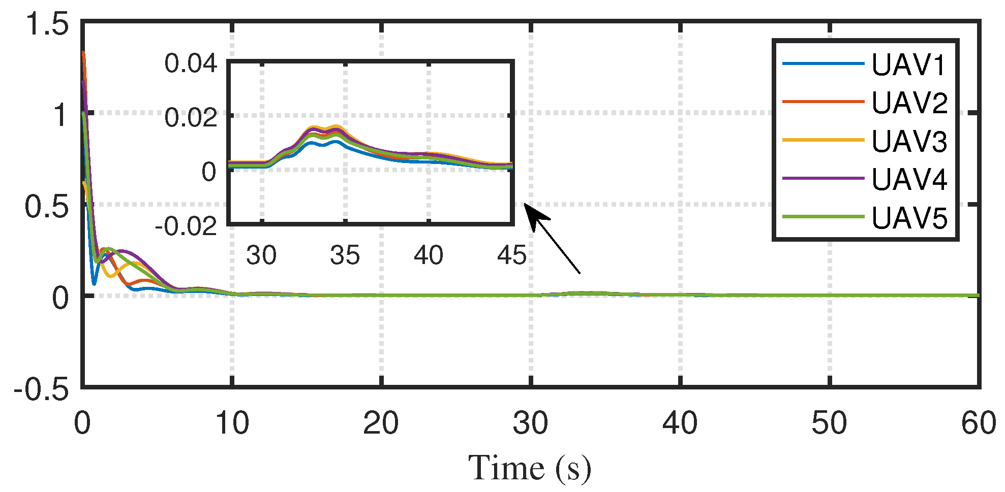
$ScenarioII$—$Externaldisturbancecase$: In this case, the desired flight trajectory are chosen as $\mathbf{n}(t)={[0.1t,0.1t,0.1t]}^T$, and the desired yaw angle ${\phi }_0=t$. The reference formation shape vectors are given by ${\mathbf{F}}_i(t)={[cos(\frac{2i\pi }{5}+\frac{\pi }{50}t),sin(\frac{2i\pi }{5}+\frac{\pi }{50}t),0]}^T$ $(i=1,\cdots ,5).$ The external disturbances are introduced into the attitude subsystem and position subsystem. We consider that the disturbances $w_{h_{i,l}}=w_{v_{i,l}}=0.15\sin (t)\cos (t)$ and $w_{m_{i,l}}=w_{n_{i,l}}=0.05{\cos }^2(t)+0.05\sin (t)$ when $t\ge 30\mathrm{s}$. The selection of formation controller parameters is the same as the above example.

Then, by using the control laws given in (22) and (40), the quadrotor UAVs’ flight trajectories in the 3-D space are displayed in Figure 8. As can be seen from Figure 8, in the presence of unknown disturbances, the five UAVs form a desired formation shape and track the desired flight trajectory. The response curves of formation tracking errors are shown in Figure 9. Obviously, the system tracking error can still converge to a very small range quickly in the presence of unknown disturbances. Thus, we can conclude that the proposed control scheme is robust to the external disturbances.

5. Conclusions

In this paper, a distributed formation tracking control method has been proposed for quadrotor UAVs. For the attitude subsystem, a cascaded ADRC method has been designed for the attitude subsystem to suppress the influence of unknown time-varying disturbances. For the position subsystem, an adaptive position control method has been devised, achieving time-varying formation tracking for quadrotor UAVs. The proposed control scheme does not need to use the model parameters of quadrotor UAVs, which has wider practicality. The effectiveness of the proposed method has been verified by a numerical example. Our future work includes time-varying formation tracking control of heterogeneous quadrotor UAVs under switched communication topologies.

References

Liu, Z.; Li, J. Application of unmanned aerial vehicles in precision agriculture. Agriculture2023, 1375. [Google Scholar] [CrossRef]
Liu, D.; Zhu, X.; Bao, W.; Fei, B.; Wu, J. SMART: Vision-based method of cooperative surveillance and tracking by multiple UAVs in the urban environment. IEEE Trans. Intell. Transp. Syst.2022, 23, 24941–24956. [Google Scholar] [CrossRef]
Liao, F.; Teo, R.; Wang, J.L.; Dong, X.; Lin, F.; Peng, K. Distributed formation and reconfiguration control of VTOL UAVs. IEEE Trans. Control Syst. Technol.2016, 25, 270–277. [Google Scholar] [CrossRef]
Li, H.; Li, X. Distributed consensus of heterogeneous linear time- varying systems on UAVs–USVs coordination. IEEE Trans. Circuits Syst. II Express Briefs2019, 27, 1264–1268. [Google Scholar] [CrossRef]
Zou, Y.; Zhou, Z.; Dong, X.; Meng, Z. Distributed formation control for multiple vertical takeoff and landing UAVs with switching topologies. IEEE/ASME Trans. Mechatron.2018, 23, 1750–1761. [Google Scholar] [CrossRef]
Huang, Y.; Meng, Z. Bearing-based distributed formation control of multiple vertical take-off and landing UAVs. IEEE Trans. Control Netw. Syst.2021, 8, 1281–1292. [Google Scholar] [CrossRef]
Pan, Z.; Zhang, C.; Xia, Y.; Xiong, H.; Shao, X. An improved artificial potential field method for path planning and formation control of the multi-UAV systems. IEEE Trans. Circuits Syst. II Express Briefs2021, 69, 1129–1133. [Google Scholar] [CrossRef]
Lee, G.; Chwa, D. Decentralized behavior-based formation control of multiple robots considering obstacle avoidance. Intell. Serv.2018, 11, 127–138. [Google Scholar] [CrossRef]
Zhou, D.; Wang, Z.; Schwager, M. Agile coordination and assistive collision avoidance for quadrotor swarms using virtual structures. IEEE Trans. Robot.2018, 34, 916–923. [Google Scholar] [CrossRef]
Dong, X.; Yu, B.; Shi, Z.; Zhong, Y. Time-varying formation control for unmanned aerial vehicles: Theories and applications. IEEE Trans. Control Syst. Technol.2014, 23, 340–348. [Google Scholar] [CrossRef]
Jiang, B.; Li, B.; Zhou, W.; Lo, L.Y.; Chen, C.K.; Wen, C.Y. Neural network based model predictive control for a quadrotor UAV. Aerospace2022, 98, 460. [Google Scholar] [CrossRef]
Romero, A.; Sun, S.; Foehn, P.; Scaramuzza, D. Model predictive contouring control for time-optimal quadrotor flight. IEEE Trans. Robot.2022, 38, 3340–3356. [Google Scholar] [CrossRef]
Li, J.; Liu, J.; Huangfu, S.; Cao, G.; Yu, D. Leader-follower formation of light-weight uavs with novel active disturbance rejection control. Appl. Math. Model.2023, 117, 577–591. [Google Scholar] [CrossRef]
Zaidi, A.; Kazim, M.; Weng, R.; Ali, S.; Raza, M.T.; Abbas, G.; Ullah, N.; Mohammad, A.S.; Al-Ahmadi, A.A. Adaptive active disturbance rejection control for rendezvous of a swarm of drones. IEEE Access2022, 10, 90355–90368. [Google Scholar] [CrossRef]
Ran, M.; Li, J.; Xie, L. Active disturbance rejection time-varying formation tracking for unmanned aerial vehicles. In Proceedings of the 2020 16th International Conference on Control, Automation, Robotics and Vision (ICARCV), Shenzhen, China, 13–15 December 2020; pp. 1298–1303. [Google Scholar]
Yao, H.; Wu, J.; Xi, J.; Wang, L. Active disturbance rejection controller based time-varying formation tracking for second-order multi-agent systems with external disturbances. IEEE Access2019, 7, 153317–153326. [Google Scholar] [CrossRef]
Hong, Y.; Hu, J.; Gao, L. Tracking control for multi-agent consensus with an active leader and variable topology. Automatica2006, 42, 1177–1182. [Google Scholar] [CrossRef]
Zuo, Z.; Wang, C. Adaptive trajectory tracking control of output constrained multi-rotors systems. IET Control Theory Appl.2014, 8, 1163–1174. [Google Scholar] [CrossRef]
Xu, L.X.; Ma, H.J.; Guo, D.; Xie, A.H.; Song, D.L. Backstepping sliding-mode and cascade active disturbance rejection control for a quadrotor UAV. IEEE/ASME Trans. Mechatron.2020, 25, 2743–2753. [Google Scholar] [CrossRef]
Chen, F.; Jiang, R.; Zhang, K.; Jiang, B.; Tao, G. Robust backstepping sliding-mode control and observer-based fault estimation for a quadrotor UAV. IEEE Trans. Ind. Electron.2016, 63, 5044–5056. [Google Scholar] [CrossRef]
Cao, Y.; Ren, W.; Meng, Z. Decentralized finite-time sliding mode estimators and their applications in decentralized finite-time formation tracking. Syst. Control Lett.2010, 59, 522–529. [Google Scholar] [CrossRef]
Figure 1.
Control block diagram of the quadrotor UAV.
Figure 2.
The communication topology.
Figure 3.
The quadrotor UAVs’ flight trajectories in the 3-D space.
Figure 4.
Actual flight formation shapes.
Figure 5.
Response curves of the attitude angles.
Figure 6.
Formation tracking errors.
Figure 7.
The quadrotor UAVs’ control inputs.
Figure 8.
Figure 9.
Disclaimer/Publisher’s Note: The statements, opinions and data contained in all publications are solely those of the individual author(s) and contributor(s) and not of MDPI and/or the editor(s). MDPI and/or the editor(s) disclaim responsibility for any injury to people or property resulting from any ideas, methods, instructions or products referred to in the content.