Structural Characteristics of a Shock Train Flow Field in a Variable Cross-Section S-Shaped Isolator

Abstract

Experiments were conducted in this study to reveal the flow characteristics of a variable cross-section S-shaped isolator, when applying the steady-state back pressure at the isolator outlet. The self-excited oscillation characteristics of the shock train generated under the influence of steady-state back pressure at an incoming flow speed of Mach 2, were also studied. The findings suggest that pressure oscillation within the area affected by the shock train’s flow field was significantly more potent than outside the affected area. Moreover, the forward movement velocity of the shock train in the variable cross-section S-shaped isolator was not uniform. The forward movement speed was slower when encountering sharp turns and faster during gentle turns. In the shock train flow field, high-frequency pressure oscillations, which mainly stemmed from the oscillations of the separated shock legs, propagated more readily within the flow field than low-frequency pressure oscillations. The significant separation of the shock train flow field will switch between the top and bottom walls, and the frequency of pressure oscillation in the large separation region is low. On another note, the closer the distance between two points is in the shock flow field, the stronger the coherence of pressure oscillations will be. In the distance upstream of the shock train flow field, the turbulent boundary layer (TBL) determines pressure oscillations instead of the shock train flow field, so the coherence was very high.

1. Introduction

An isolator is a crucial part located between the inlet and combustor of a scramjet. Its primary function is to isolate the influence of the combustor on the inlet and prevent the backpressure of the combustor from causing the inlet not to start. In addition, the shock train in the isolator can slow the supersonic flow to achieve high pressure. The structure length of the shock train, the static pressure recovery characteristics, and the total pressure recovery characteristics influence the isolator’s performance considerably; in extension, these factors also impact the performance of the scramjet.

The isolator configuration was generally simple during the scramjet’s early development stage. Further, researchers extensively studied the cylindrical cuboid isolators and equal sections. Researchers have investigated the flow structure of shock trains and the static pressure distribution characteristics along the path and conducted numerical simulations. Waltrip and Billig [1,2,3,4] laid the foundation for more extensive research. In the context of integrated design requirements, when the inlet and the combustion-chamber inlet of the engine are spatially biased, and their shapes are inconsistent because of the requirements of the overall layout and aerodynamic characteristics, a traditional isolator cannot satisfy the design requirements, and the variable cross-section S-shaped isolator must be used to match the engine flow passage. Recently, some scholars have modified the traditional isolator model with an S-shaped isolator section. These theories are based on experimental data fitting and lack a physical basis. Additionally, these theoretical models are mainly based on zero-dimensional analysis of equally straight pipes unsuitable for capturing shock wave characteristics in pipelines with a variable cross-sectional area.

For the variable cross-section isolator with no change in axis (the centroid of any cross-section of the isolator is on the same axis), scholars have studied it. Tian Xuang [5] designed two kinds of variable cross-section isolators; based on the hyperelliptic curve, Gao Liangjie [6] designed square-to-circle isolators with different cross-section variations. Tan Huijun [7] et al. studied the wall pressure oscillation characteristics in the two-dimensional S-shaped isolator. Chen Jingfan [8] used the geometric fusion method to design the variable cross-section isolator of the crescent turning circle with a variable section.

Tan Huijun and Guo Rongwei [7] studied the structural characteristics of the flow field in the two-dimensional curved isolator. The results showed that the performance of the constant section straight isolator was better than that of the S-shaped isolator at a relatively low-pressure ratio. However, the difference between them decreased when the pressure ratio increased. Moreover, for the shock train length in the isolator shock train, the length in the S-shaped isolator is shorter than that in the constant-section straight isolator.

Wang Chengpeng [9] studied the isolator of the octagon section and found that compared with the traditional shape (circular section and rectangular section), the shock train length in the isolator of the octagon section was shorter. Ding Meng and Li Hua [10] conducted a simulation study on the two-dimensional rectangular isolator. They found that the B-L algebraic turbulence model did not apply to flows with large separation areas. Wang Dongping and Zhao Wenzhong [11] conducted a numerical simulation of a shock train during Mach 4 flow and took high-speed colour schlieren photography. The results showed that the first oblique shock wave in Mach 4 flow appeared asymmetry, which may be caused by the different thicknesses of the boundary layer on the top and bottom walls. Gao Liangjie [6] studied the variable cross-section isolator with a square entrance and circular exit, and the results indicate that the isolator with proper section change performs best. Either too fast or too slow section transition is not beneficial to the improvement of the performance of the isolator. Guo Shanguang [12] studied the isolator under different backpressure conditions and found hysteresis with the change in back pressure. Li Tengji [13] further conducted simulation and experimental studies on the S-shaped isolator. The results showed that the two reasons for the hysteresis phenomenon were the initial pressure distribution along the wall and the self-sustaining characteristics of the separation zone.

Zhang Hang [14] studied the three-dimensional S-shaped isolator and found that the swirling flow generated by the corner area in the section developed continuously with the flow, eventually causing severe distortion of the flow field at the exit section. Xiong Bing [15,16] studied the flow characteristics of the shock train flow field in the S-shaped isolator under the inflow condition of Mach 2, and the study showed that there were two hysteresis phenomena in the isolator and the self-excited oscillation phenomenon of shock wave string was more likely to occur in the S-shaped isolator. Huang [17] conducted an experimental study on the two-dimensional S-shaped isolator, indicating that the downstream curvature of the isolator is inversely proportional to the separation size. In order to study the influence of boundary layer thickness at the inlet of the isolator on the S-shaped isolator, An Bin [18] designed three different S-shaped isolators for research. Tan [19] found that for the S-shaped isolator, the length of the internal shock train was longer than that of the constant section straight isolator.

2. Experimental Design and Numerical Calculation

2.1. Numerical Simulation Method

The governing equations for the numerical calculation are mass, momentum, and energy equations, as follows:

$$\frac{\partial \rho }{\partial t}+\nabla \left(\rho \overrightarrow{u}\right)=0$$

(1)

$$\frac{\partial \left(\rho u\right)}{\partial t}+\nabla \left(\rho u\overrightarrow{u}\right)=-\frac{\partial p}{\partial x}+\frac{\partial {\tau }_{xx}}{\partial x}+\frac{\partial {\tau }_{yx}}{\partial y}+\frac{\partial {\tau }_{zx}}{\partial z}+\rho f_x$$

(2)

$$\frac{\partial \left(\rho v\right)}{\partial t}+\nabla \left(\rho v\overrightarrow{u}\right)=-\frac{\partial p}{\partial y}+\frac{\partial {\tau }_{xy}}{\partial x}+\frac{\partial {\tau }_{yy}}{\partial y}+\frac{\partial {\tau }_{zy}}{\partial z}+\rho f_y$$

(3)

$$\frac{\partial \left(\rho w\right)}{\partial t}+\nabla \left(\rho w\overrightarrow{u}\right)=-\frac{\partial p}{\partial z}+\frac{\partial {\tau }_{xz}}{\partial x}+\frac{\partial {\tau }_{yz}}{\partial y}+\frac{\partial {\tau }_{zz}}{\partial z}+\rho f_z$$

(4)

$$\frac{\partial }{\partial t}\left[\rho \left(e+\frac{{\overrightarrow{u}}^2}{2}\right)\right]+\nabla \left[\rho \left(e+\frac{{\overrightarrow{u}}^2}{2}\right)\overrightarrow{u}\right]=p\dot{q}-\frac{\partial \left(up\right)}{\partial x}-\frac{\partial \left(vp\right)}{\partial y}-\frac{\partial \left(wp\right)}{\partial z}+\frac{\partial }{\partial x}\left(k\frac{\partial T}{\partial x}\right)+\frac{\partial }{\partial y}\left(k\frac{\partial T}{\partial y}\right)+\frac{\partial }{\partial z}\left(k\frac{\partial T}{\partial z}\right)+\frac{\partial \left(u{\tau }_{xx}\right)}{\partial x}+\frac{\partial \left(u{\tau }_{yx}\right)}{\partial y}+\frac{\partial \left(u{\tau }_{zx}\right)}{\partial z}+\frac{\partial \left(v{\tau }_{xx}\right)}{\partial x}+\frac{\partial \left(v{\tau }_{yx}\right)}{\partial y}+\frac{\partial \left(v{\tau }_{zx}\right)}{\partial z}+\frac{\partial \left(w{\tau }_{xx}\right)}{\partial x}+\frac{\partial \left(w{\tau }_{yx}\right)}{\partial y}+\frac{\partial \left(w{\tau }_{zx}\right)}{\partial z}+\rho \overrightarrow{f}·\overrightarrow{u}$$

(5)

In the mass Equation (1), $\rho ,t$,$\overrightarrow{u}$,$\nabla$ Are the fluid density, time, velocity vector, and divergence, respectively. In the momentum conservation Equations (2)–(4), $\tau$ is the shear stress, u is the velocity component in the x direction, v is the velocity component in the y direction, and w is the velocity component in the z direction, $f$ is the body force, p is the pressure. In the energy Equation (5) of the fluid, k, T, $\dot{q}$ were thermal conductivity, temperature, and heat flux, respectively, velocity component.

The turbulence model is the $SST K-\omega$ model, $SST K-\omega$ model is referred to as the shear stress transport model. In this model, the $K-\omega$ formula is applied near the boundary layer so that the model can be directly calculated to the viscous bottom layer so that the $SST K-\omega$ model can be used as a low Reynolds number model without an extra damping formula. On the other hand, the model switches to the $K-\epsilon$ model in the fully developed flow region, which avoids the problem that the $K-\omega$ model is too sensitive to the turbulence of the inlet flow.

Boundary conditions of far-field conditions and stress conditions are adopted. Use the stress condition of far-field as the free boundary condition of infinity, mainly setting the project to the free stream Mach number and static parameters. Using pressure requirements to assume far-field boundary conditions for ideal gas density calculation in order to meet the requirements of infinity, choose this kind of boundary condition request object distance far enough. The pressure outlet condition defines the static pressure on the outlet boundary of the flow field. When the flow field on the boundary reaches supersonic speed, the pressure on the boundary will be obtained through the internal interpolation of the flow field. Reflux conditions should also be defined on the boundary of the pressure outlet.

To analyse the near-wall flow, the height of the first layer grid is 0.001 mm. Use the Second Order Upwind for the dispersion, and set the air as an ideal gas. Use the Sutherland formula to calculate the molecular viscosity. The wall conditions were adiabatic, solid, and no-slip conditions.

In order to verify the correctness of the numerical simulation method in this paper, select the classical experiment of Kawatsu [20] for verification. Kawatsu’s experimental model is a rectangular section with a length of 290 mm and a cross-section with a height of H = 30 mm, which is a constant section straight isolator. The total pressure is 100 kPa, the total temperature is 298 K, and the pressure ratio Pb/Pi is 3.8. As shown in Figure 1, the simulation results agree with the experimental results, proving that the numerical calculation method selected in this paper is accurate and reliable.

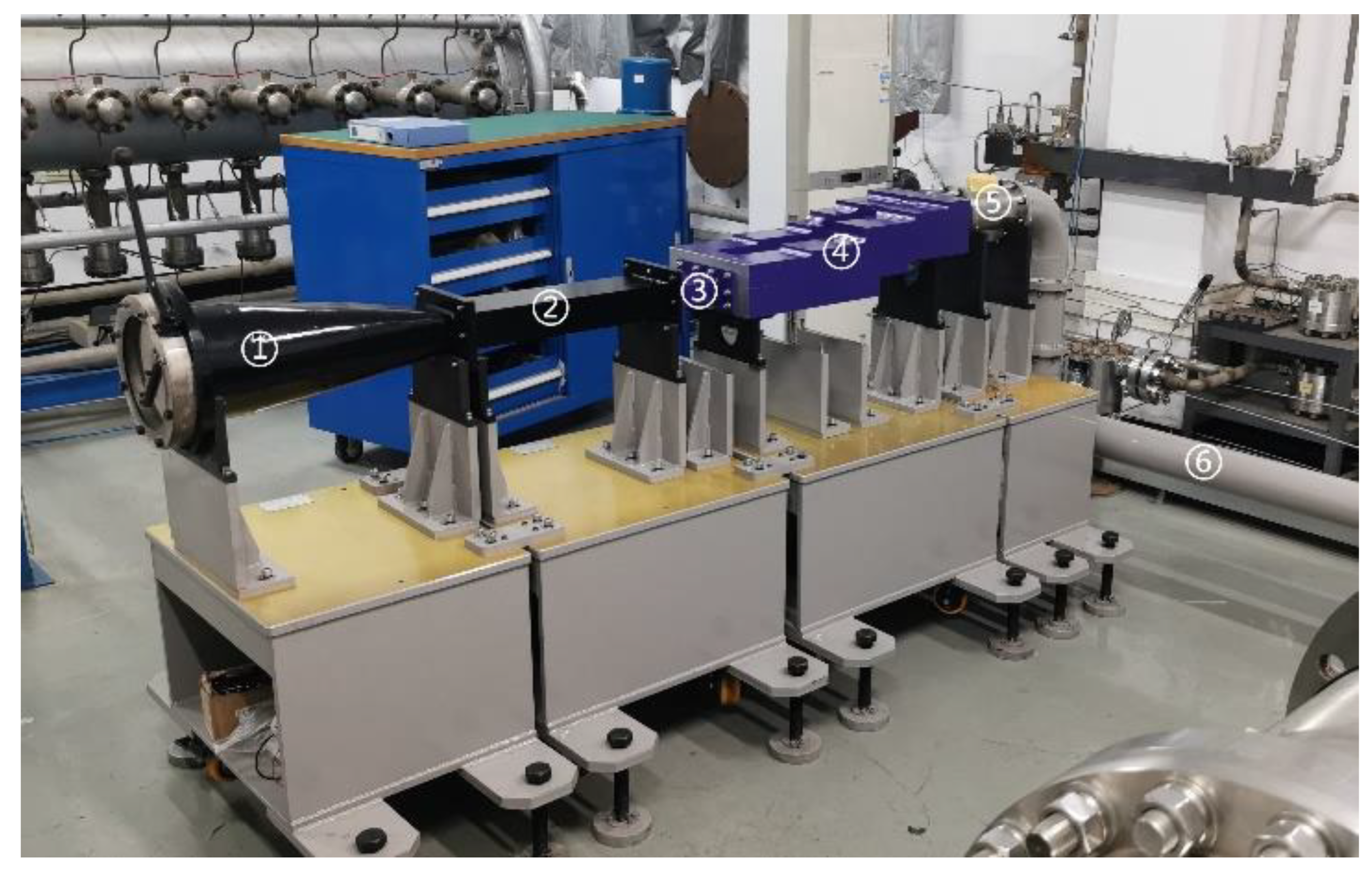
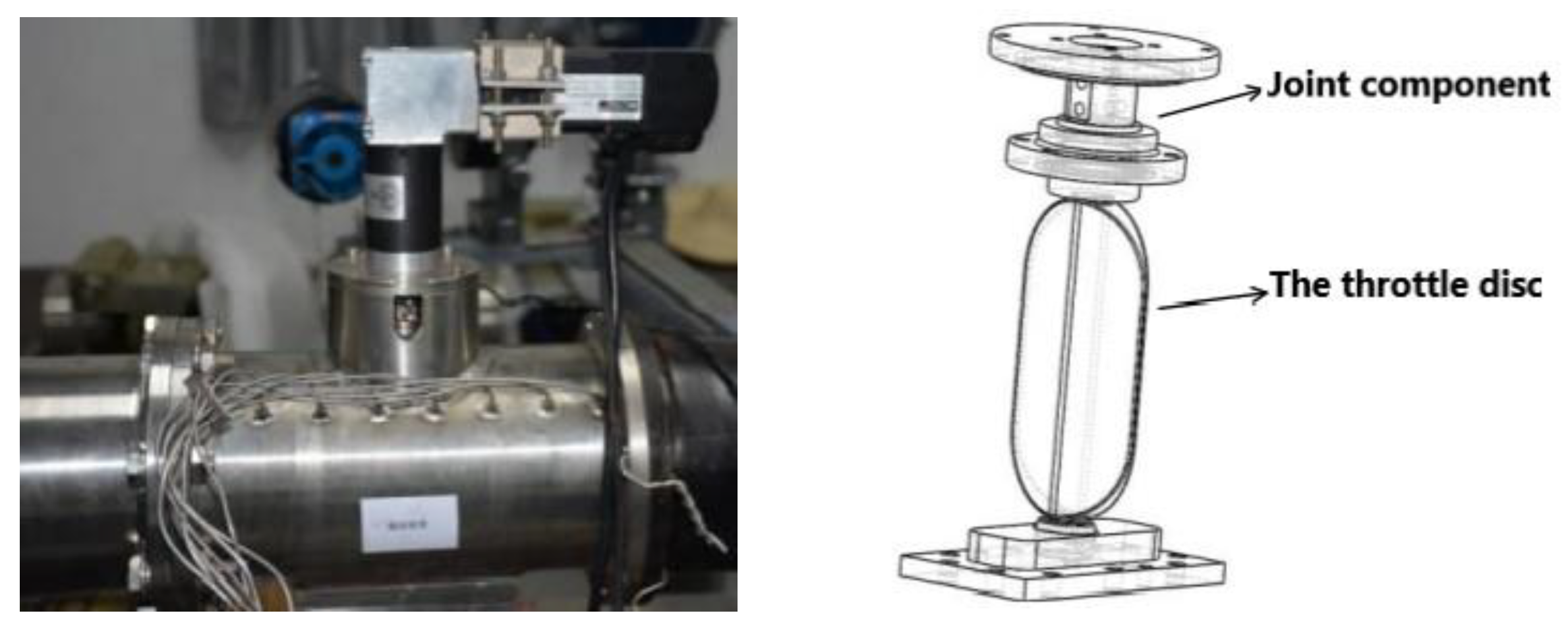
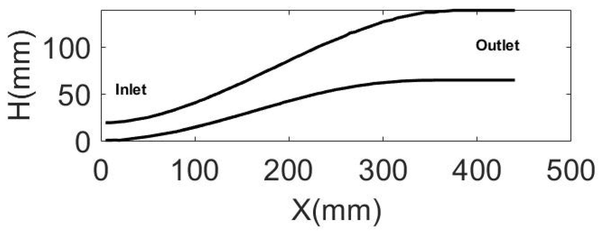
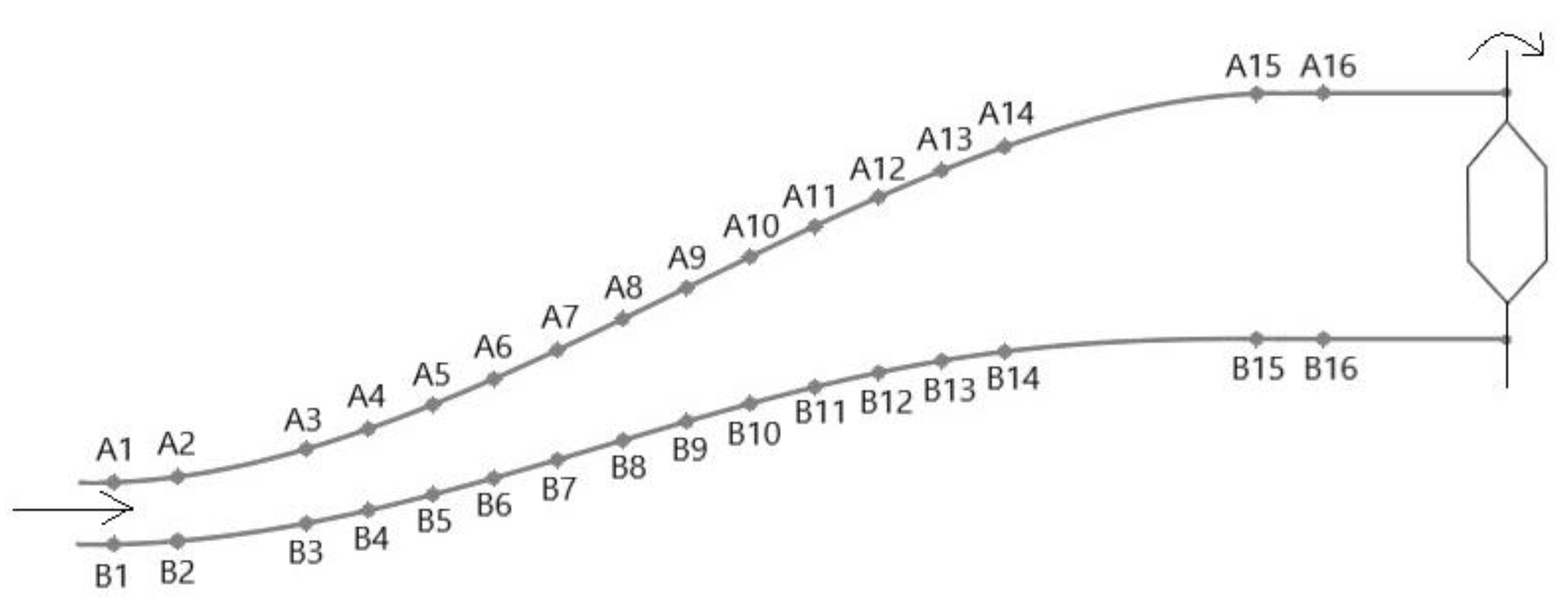
2.2. Experimental Design

The experiment in this article was performed in an air-breathing hypersonic ramjet key laboratory at the National University of Defence Technology using a supersonic wind tunnel (Figure 2). The critical parts of the wind tunnel include: (1) a gas section, (2) stable section, (3) Mach 2 nozzle, (4) test section, (5) steady-state throttle, and (6) airway tube to the vacuum chamber. The large diameter gathering section at the wind tunnel’s entrance helps collect atmospheric air and make the incoming flow more uniform. The stable section stabilizes the incoming flow. The nozzle section is a Laval nozzle with a fixed profile, and the transfer section realizes the function of a square crescent such that the test section and steady throttle section are connected. A throttling disc is arranged inside the steady throttling section, which can adjust the backpressure at the outlet of the isolator section. The steady throttling section mainly comprises a throttling disc, servo motor, controller, and control computer.

The throttling disc is installed inside the cylinder. One end is connected to the rotating shaft of the driving motor and locked with a locking screw, and the other is placed in the concave of the blocking cover under the throttle cylinder. A motor drives the throttle disc to rotate with a fixed axis in the throttle barrel, and its rotation angle and speed are calculated. Machine precise control can adjust the clogging degree according to the test needs. The throttling disc used in this test can be solid. The rotation range is 360 degrees, the speed range is one degree/s–180 degrees/s, and the plugging degree is adjustable. The plugging degree was calculated as the ratio of the projected area of the throttle disc on the pipe’s cross-section to the pipe’s cross-section. Figure 3 shows the physical diagram of the throttle cylinder and the structure diagram of the throttle disc in the throttle cylinder. It is then connected to the vacuum chamber via the airway tube section, and the vacuum chamber downstream is connected to the vacuum sphere. Figure 4 shows the transversal dimensions of the channel cross-section. Figure 5 is the sensor distribution diagram on the isolator, and

Table 1. Sensor position distribution.

Sensor	A1, B1	A2, B2	A3, B3	A4, B4	A5, B5	A6, B6	A7, B7	A8, B8	A9, B9	A10, B10	A11, B11	A12, B12	A13, B13	A14, B14	A15, B15	A16, B16
x (mm)	7	27	67	87	107	127	147	167	187	207	227	247	267	287	367	387

is the corresponding x coordinate of the sensor.

This experiment’s high-frequency pressure measurement system is mainly composed of the NS-2 pressure sensor and digital acquisition equipment. NS-2 small pressure sensor has a fully sealed structure with an M5 × 0.5 threaded interface, which is easy to install and use and has the advantage of small size, being lightweight, and with high reliability. It can measure non-corrosive gases and liquids and has many applications. Its main working parameters are as follows: range: 200 kPa; working voltage: 5 VDC; integrated accuracy: ±0.25% F.S.

High-frequency pressure sensors directly measure the strain in strain gauges and cannot directly measure pressure, so they must be calibrated before use. Since the sensor has an excellent linear relationship, it is only necessary to determine the linear relationship between pressure and strain.

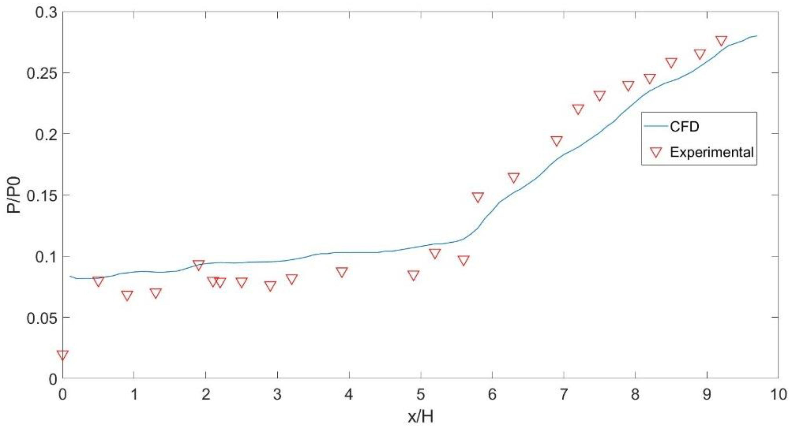
2.3. Experimental Verification of the Numerical Calculations

Figure 6 shows the experimental and simulation comparison without back pressure. Figure 7 shows the experimental and simulation comparison with the back pressure condition that Pb/P1 is three. Non-dimensional treatments for the experimental data are produced in the analysis process. P1 is the inlet pressure of the isolator. L is the length of the isolator.

The “plugging degree” measures the size of the backpressure in actual experimental operation, mainly referring to the degree of blockage of the flow channel by the downstream throttle disc. In simulation calculations, the backpressure ratio is generally used to indicate the magnitude of the backpressure applied at the outlet, meaning the ratio of the pressure applied at the outlet to the total pressure of the incoming flow. In this paper, the position of the leading edge of the shock train in the isolator is used to determine whether the two are equal. When the leading edge of the shock train in the corresponding flow field is the same, the backpressure ratio of the isolation section under the plugging degree condition is considered the same as the backpressure ratio calculated in the simulation.

However, in specific experiments, it is often impossible to precisely locate the position of the leading edge of the shock train, so it is only when the leading edge of the shock train is located precisely at a particular sensor position that we can quantitatively measure what the backpressure ratio corresponding to the plugging degree is. In Figure 7, the position of the leading edge of the shock train at a backpressure ratio of three is consistent with the experimental flow field at a downstream plugging degree of 38.36%.

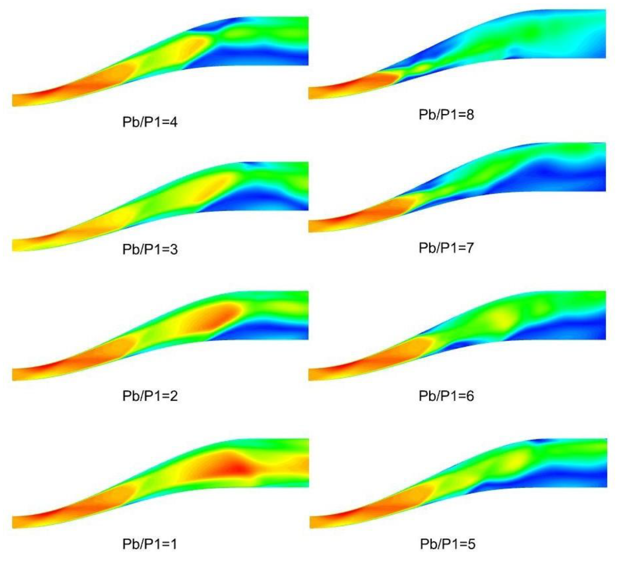
3. Self-Excited Oscillation Characteristics of a Shock Train in an Isolator

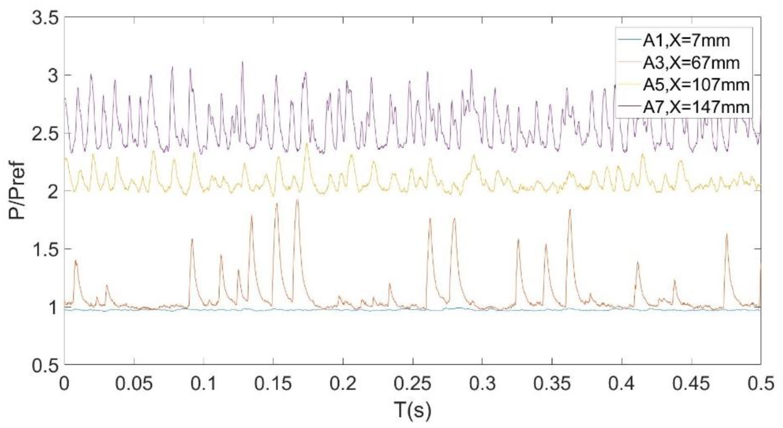
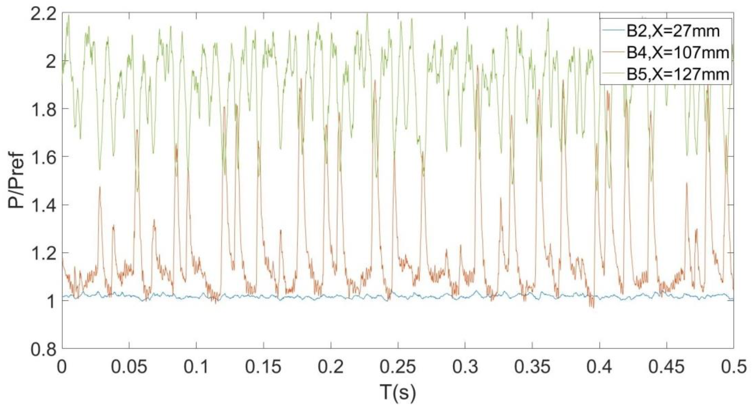
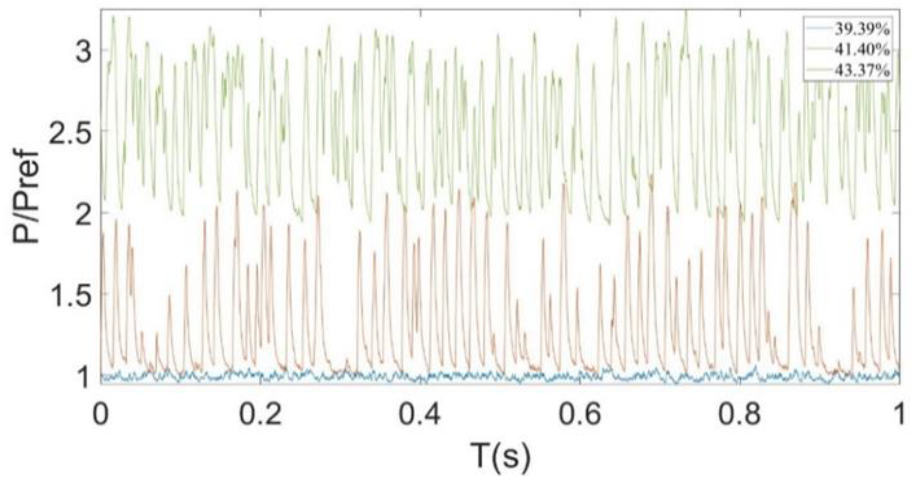
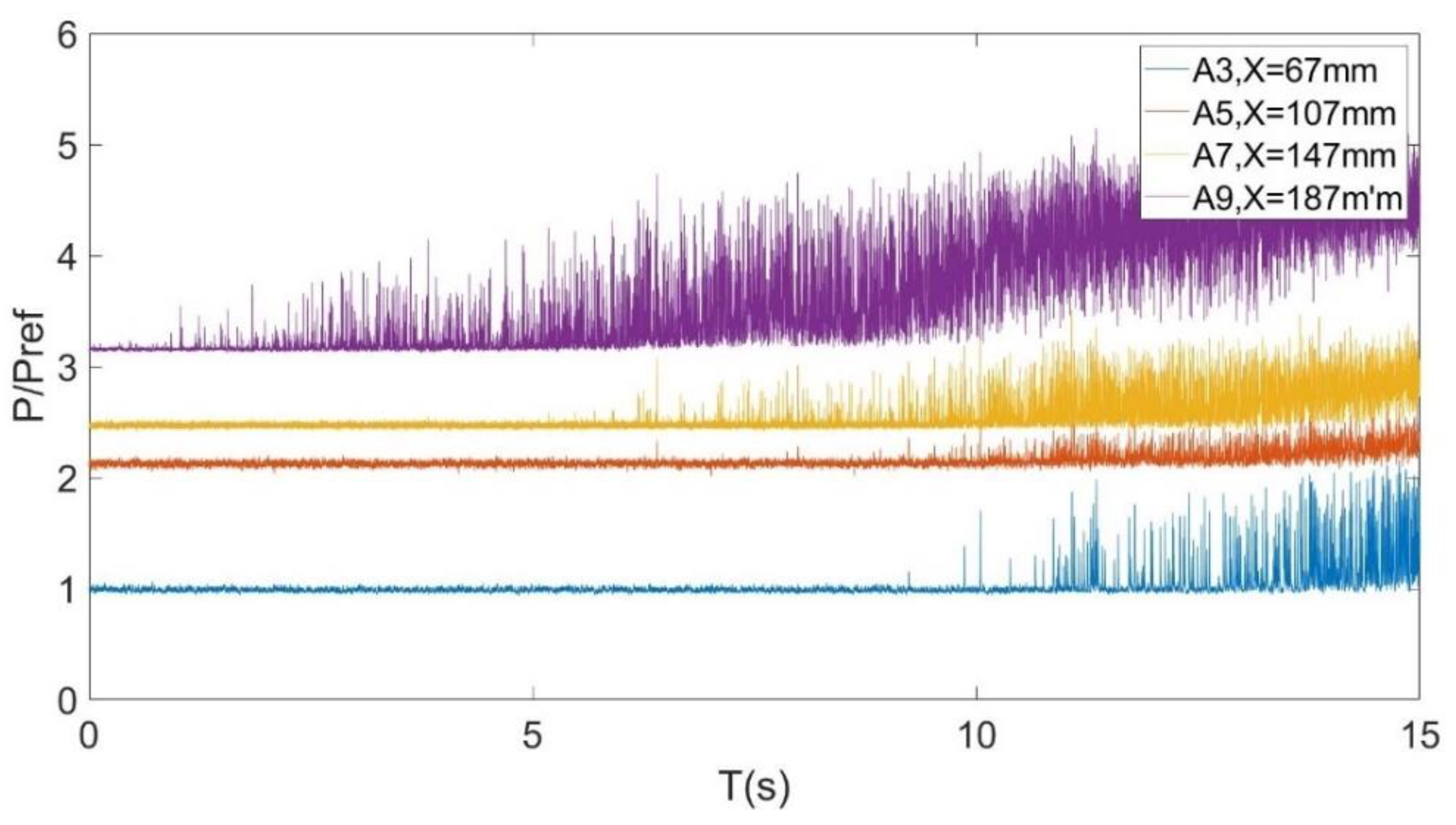
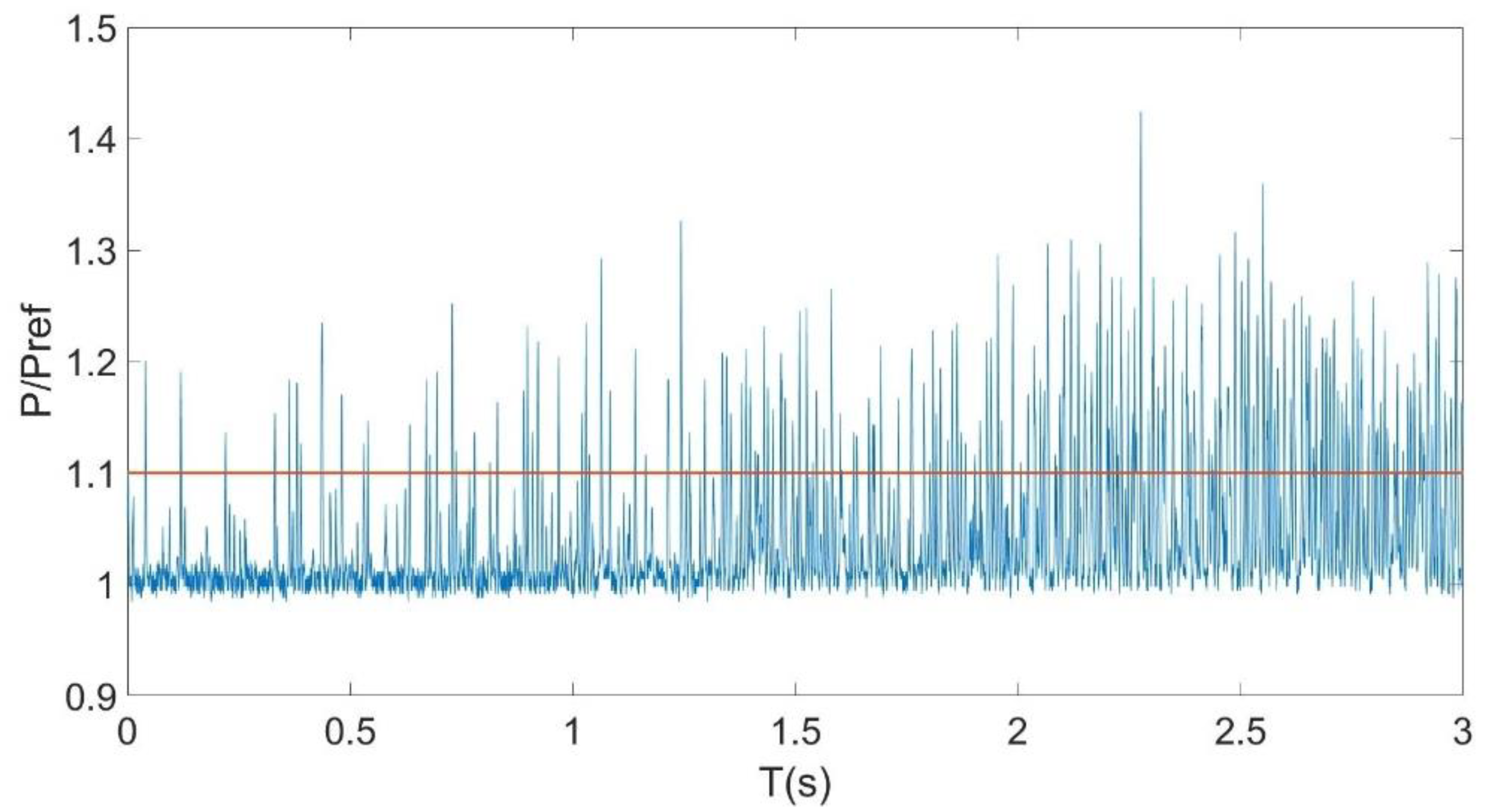
3.1. Pressure Fluctuation Characteristics of a Shock Train

Figure 8 shows the dimensionless pressure-time curves of Measuring Points A1, A3, A5, and A7 under the downstream plugging degree is 41.40%. The reference pressure Pref is the hourly average pressure value of Sensor A1, which is 9 kPa. The pressure of Pressure Sensor A1 at the entrance of the isolator has nearly no oscillation because this point is located far upstream of the shock train and is barely affected by the shock train flow field. However, the pressure of Sensor A3 oscillates and is intermittently greater than the undisturbed pressure value, indicating that the shock train leading edge continuously passes through this point because of the self-excited oscillation of the shock train. This point is located at the leading edge of the shock train. The pressure measured by Pressure Sensor A7 oscillates up and down around the time average pressure value, demonstrating that this point is in the shock train flow field under this plugging degree. Because of the self-excited oscillation of the shock train, the bifurcated shock leg constantly sweeps across Measurement Point A7, causing its pressure to oscillate violently. The pressure at Sensor A5 also oscillates; however, the amplitude is smaller than that at A7, implying that this point is between two shock waves.

Figure 9 shows the dimensionless pressure–timing curves of Sensors B2, B4, and B5 located on the bottom wall when the downstream plugging degree was 41.40%. The reference pressure Pref is the average pressure value of Sensor B2, which is 12 kPa. According to the analysis of the top wall, B4 is located at the leading edge of the shock train on the bottom wall. Because Sensors A3 and B4 are not at the same flow position, the shock shape in the variable section isolator is asymmetry.

Figure 10 presents the dimensionless pressure–timing oscillation curve of Sensor A3 under three different plugging degree conditions. Pref is the mean pressure value when the plugging degree is 39.39% (9 kPa). When the plugging degree is 39.39%, the measuring point is located far upstream of the shock train flow field, the flow is nearly constant, and the oscillation can be neglected. When the plugging degree is 41.40%, the pressure oscillates markedly. It becomes intermittently higher than the value before the disturbance demonstrating that the shock train front passes through this point intermittently. Under this condition, sensor A3 is located at the front edge of the shock train flow field. When the plugging degree reaches 43.37%, the pressure at this point fluctuates violently, oscillating around the mean value of time. This point is already in the shock train flow field, and the shock leg continuously sweeps across the measuring point, causing violent pressure oscillation.

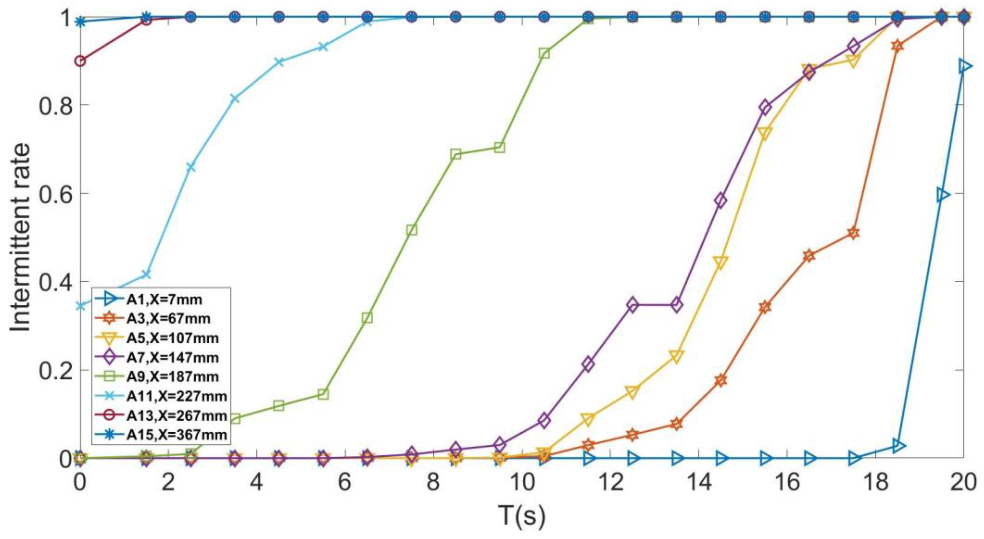
3.2. The Law of Forward Movement of Shock Train Leading Edge under the Back Pressure

Figure 11 shows the Mach number diagram of the symmetric plane with the backpressure at the outlet of the isolator increasing from 1 times the total inflow pressure to 8 times (the maximum backpressure multiple that the isolator section can withstand). It can be seen from the figure that with the continuous increase of the backpressure multiple, the leading edge of the shock train also moves forward. At the same time, there will be a separation region at the top wall and the bottom wall.

Figure 12 shows each sensor’s dimensionless pressure oscillation image on the top wall under the condition of slowly increasing the downstream plugging degree. The disc of the rotating backpressure application device rotates one degree per second. Pref is 9 kPa for the time average pressure value of Sensor A3 when it is not affected by the shock train flow field. The closer to the downstream pressure sensor, the earlier the pressure oscillation occurs. With the shock train’s forward movement, the sensor’s pressure oscillation is gradually violent, and the time average of the pressure is also gradually increased.

To facilitate the analysis of the propagation characteristics of the shock train front in the isolator, a parameter, intermittent rate, is defined to quantitatively compare the sequence of detecting the shock train front by each sensor. The intermittent rate is defined as the ratio of the duration during which the pressure fluctuation detected by a particular sensor is greater than the pressure fluctuation threshold and the total time.

Figure 13 shows the intermittent rate of the wall pressure oscillation under the throttling degree from 35.22% to 43.37%. As Figure 10 shows, the pressure fluctuation threshold is defined as 1.1 times the average pressure oscillation time under the condition that the sensor is not affected by the shock train flow field. The time window used to analyse the intermittent rate was set as one second, and the intermittent rate of 0.4 was taken as the arrival of the front edge of the shock wave series. As shown in Figure 14, the sensor closer to the exit of the isolator section detects the arrival of the leading edge of the shock train earlier. The propagation speed of the shock train in the isolator when the disc of the downstream backpressure application device rotates at a constant speed of one degree per second is illustrated in

Table 2. Forward velocity of the shock train at different positions.

Location	A1–A3	A3–A5	A5–A7	A7–A9	A9–A11
Speed (mm/s)	12.70	23.26	71.43	5.87	6.97

. Consequently, the shock train’s propagation speed in the variable section isolator is not constant, instead propagating slowly in the area of rapid turning and fast in the area of gentle turning.

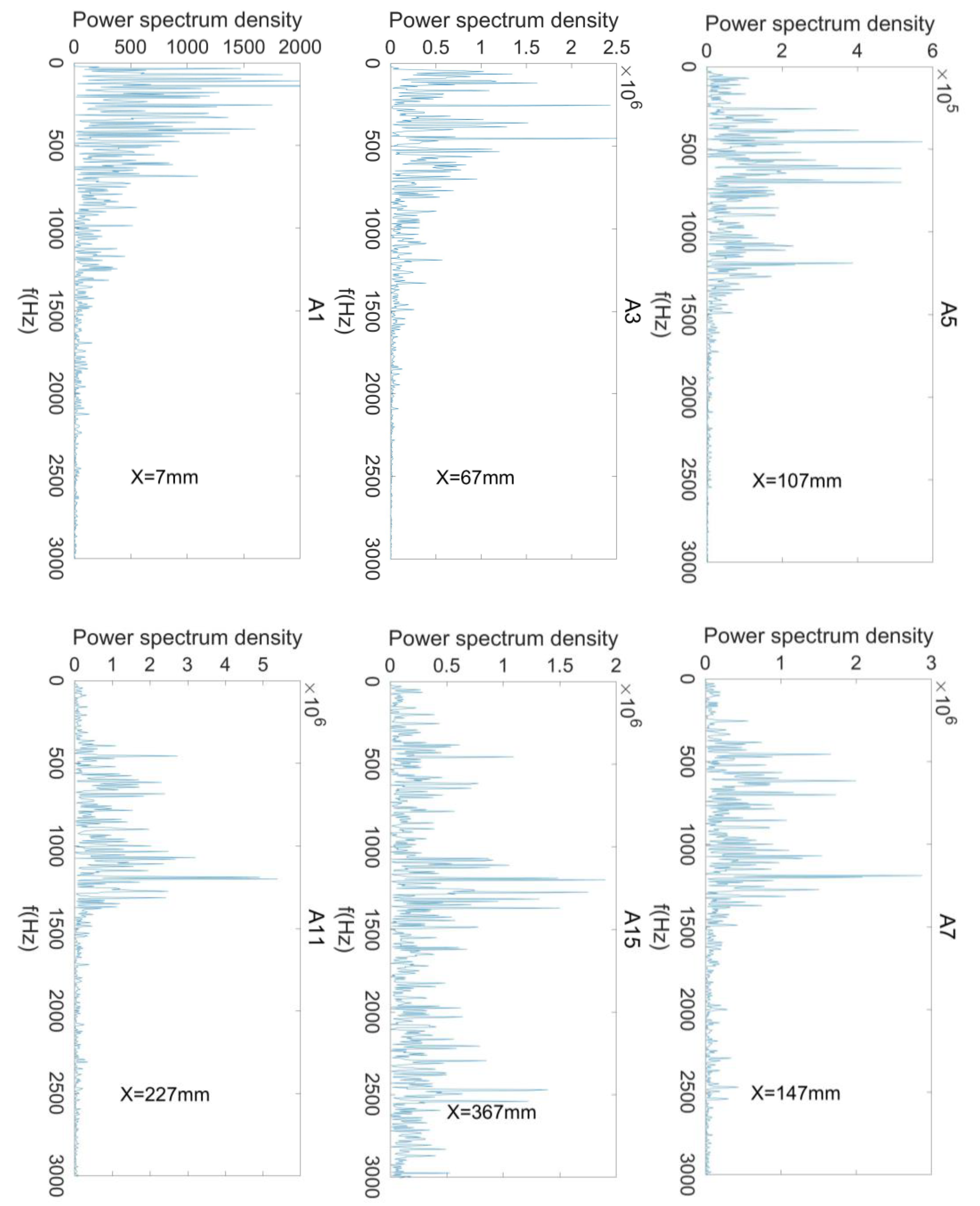
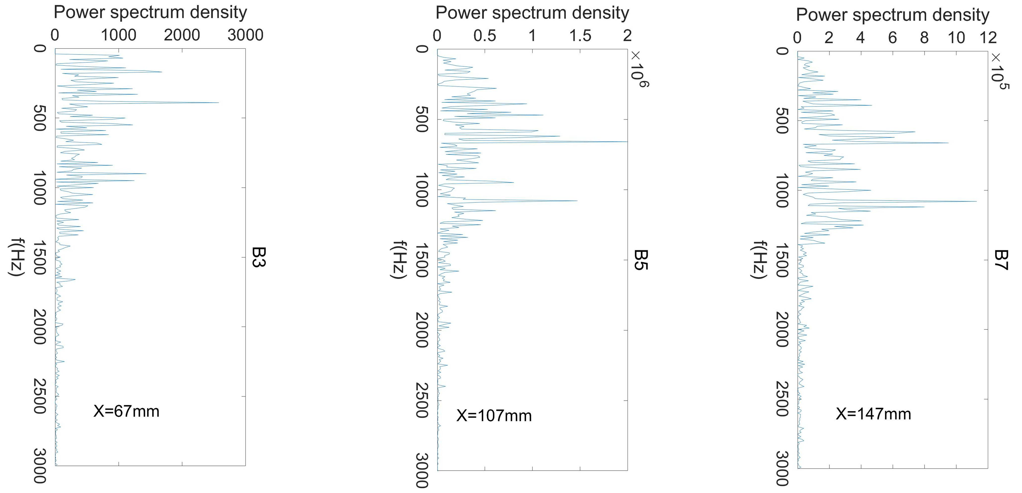
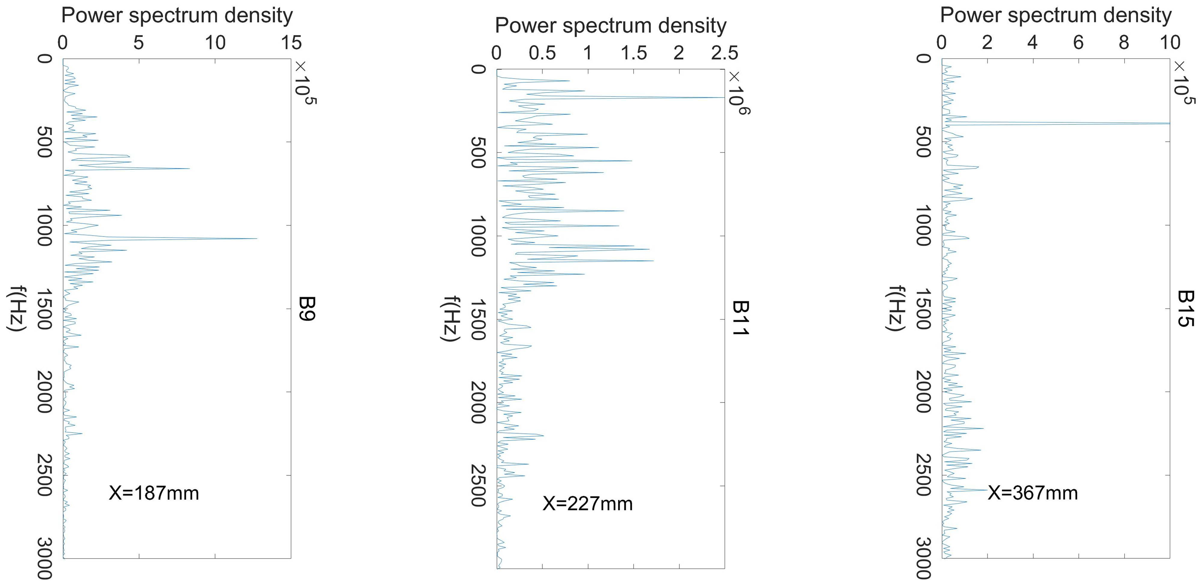
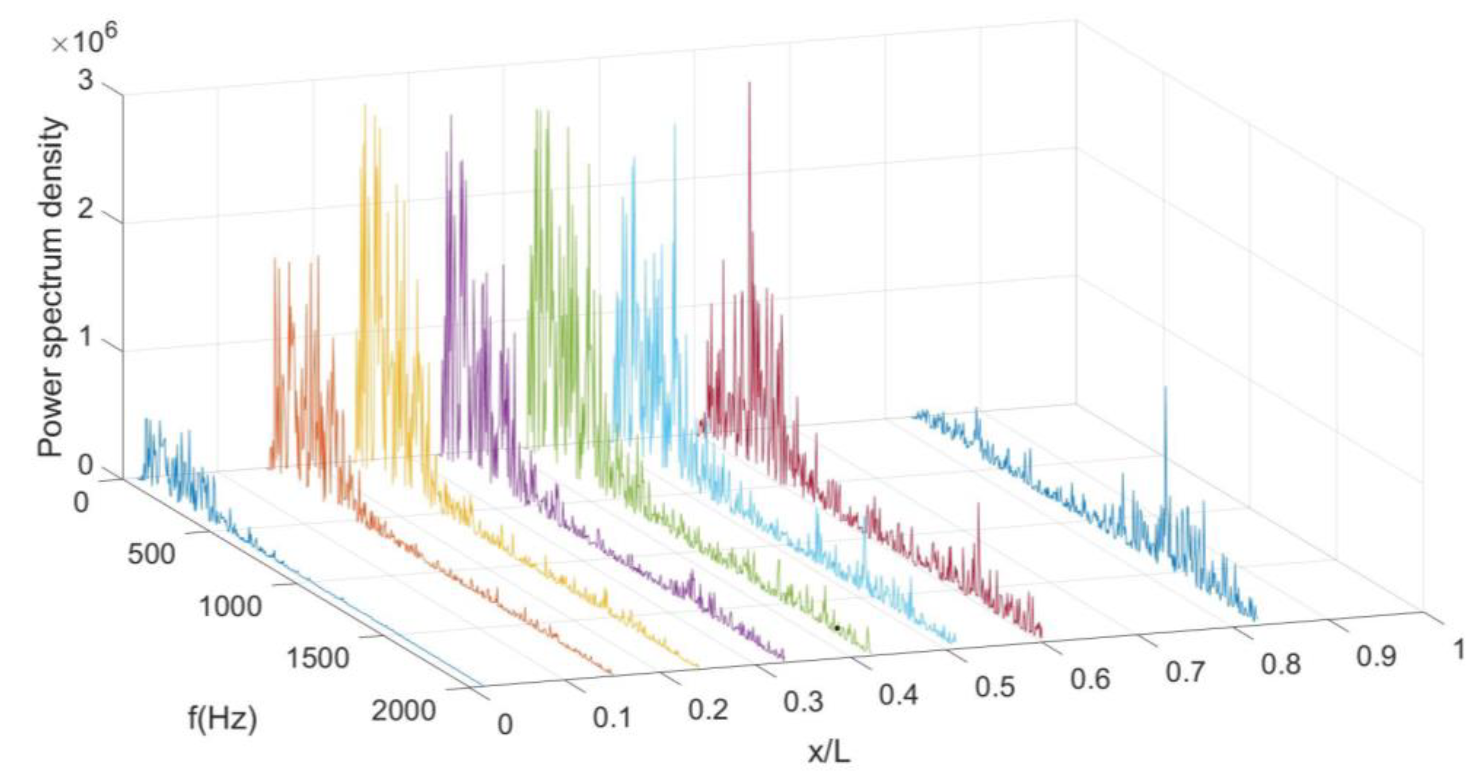
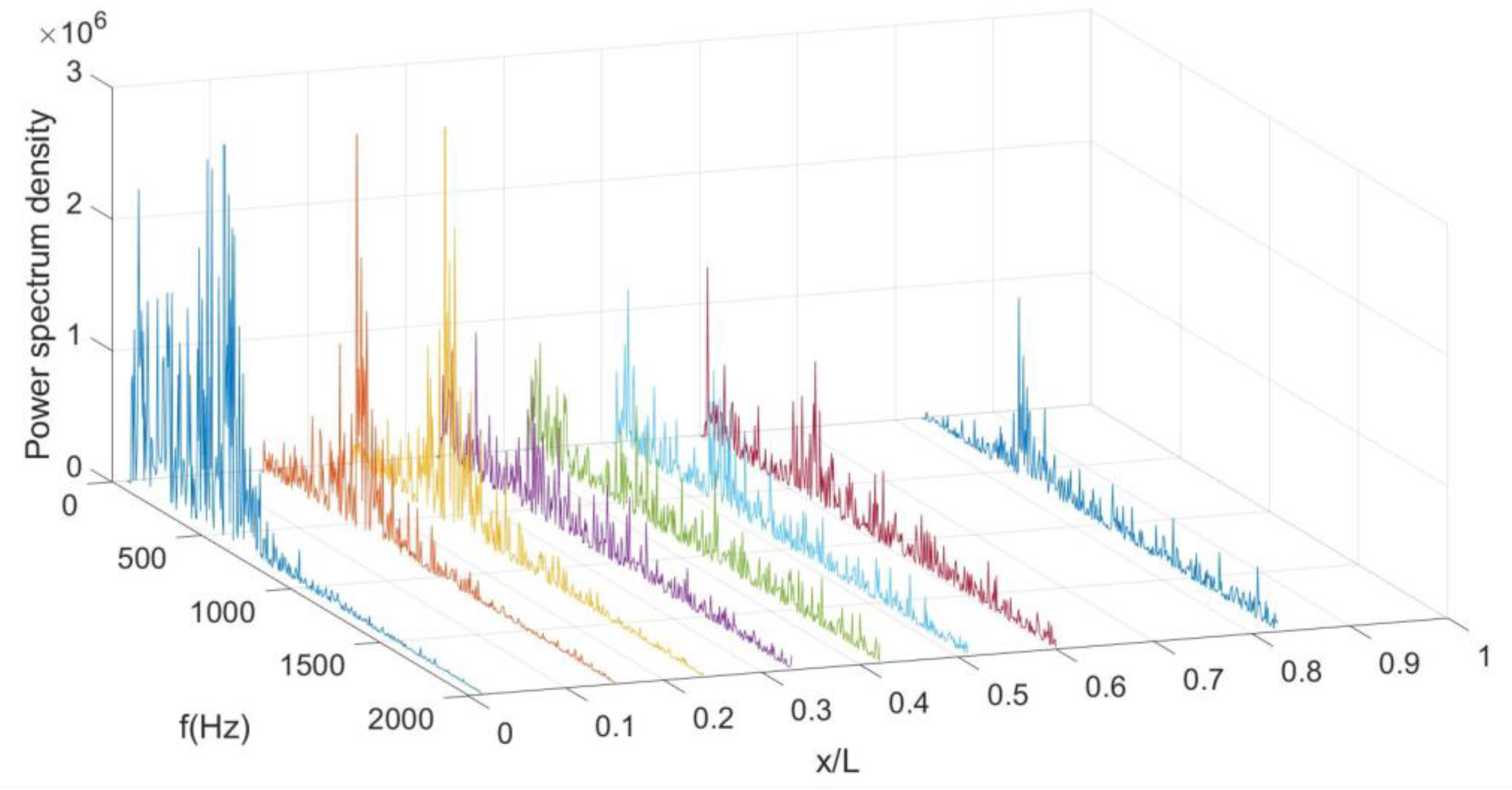
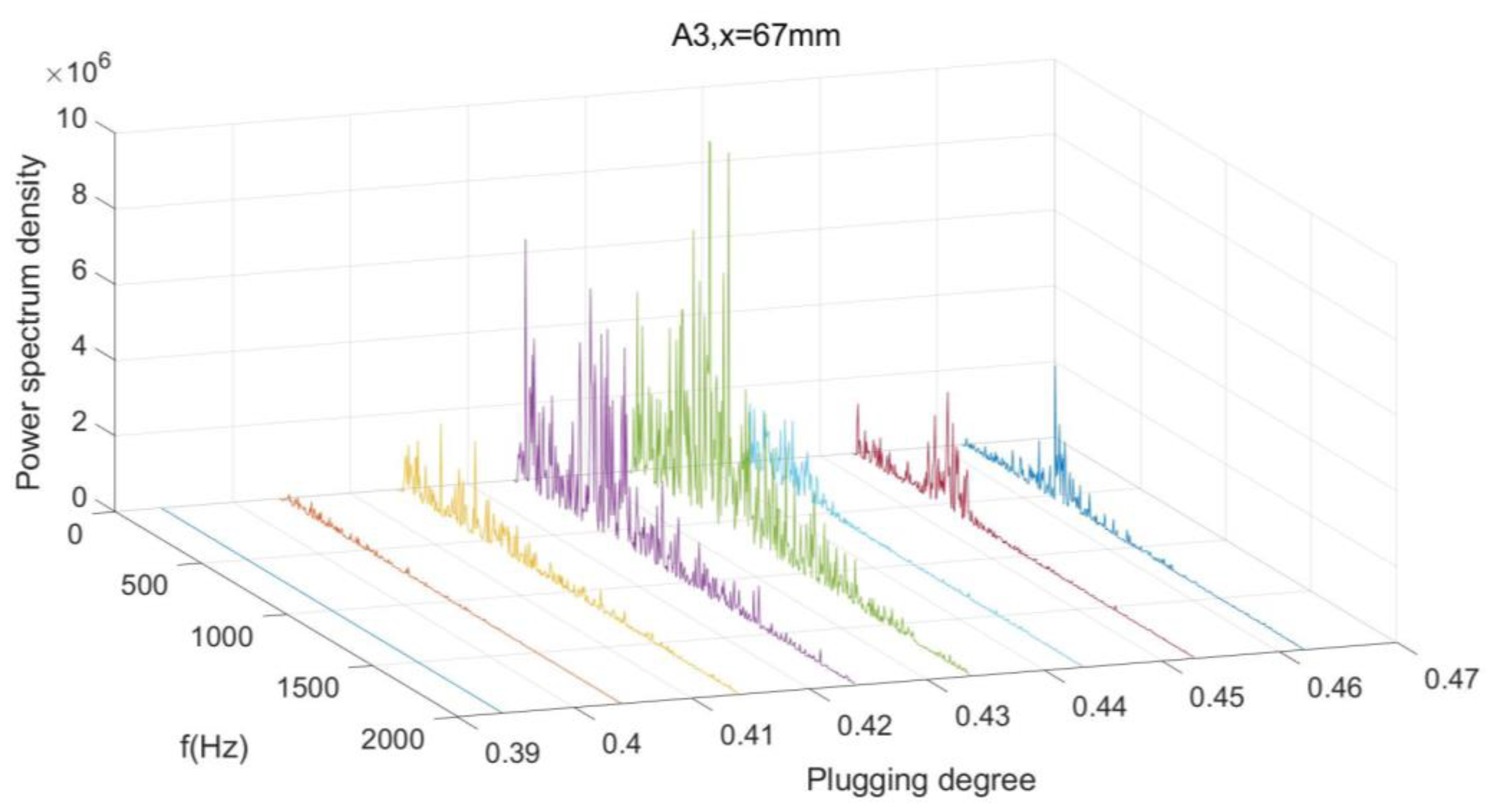
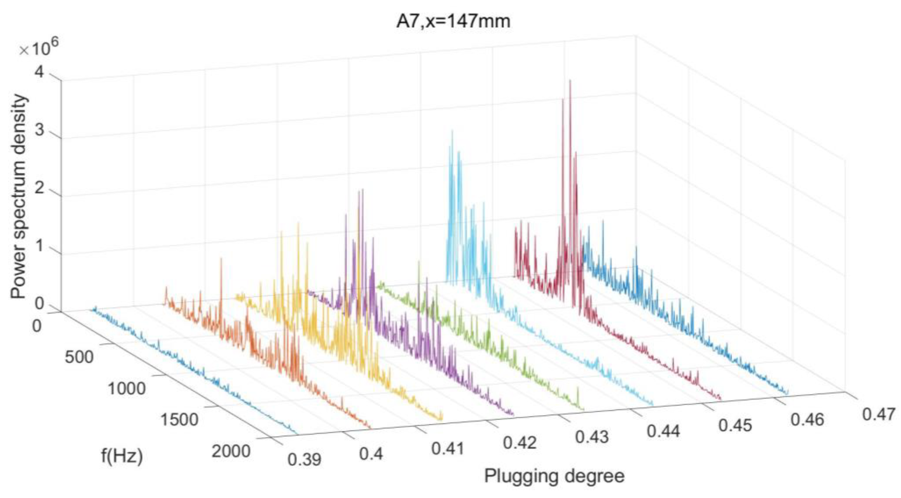
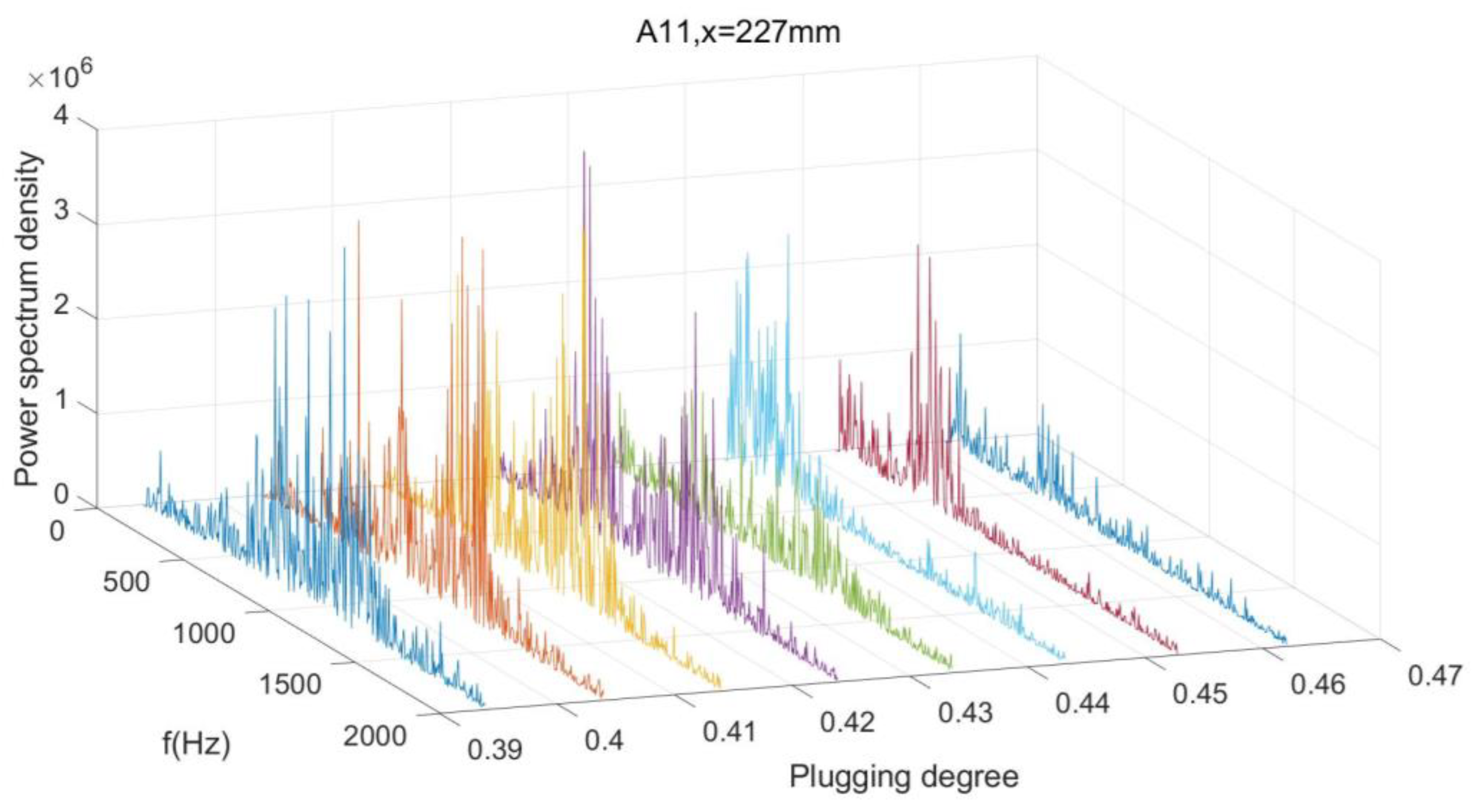
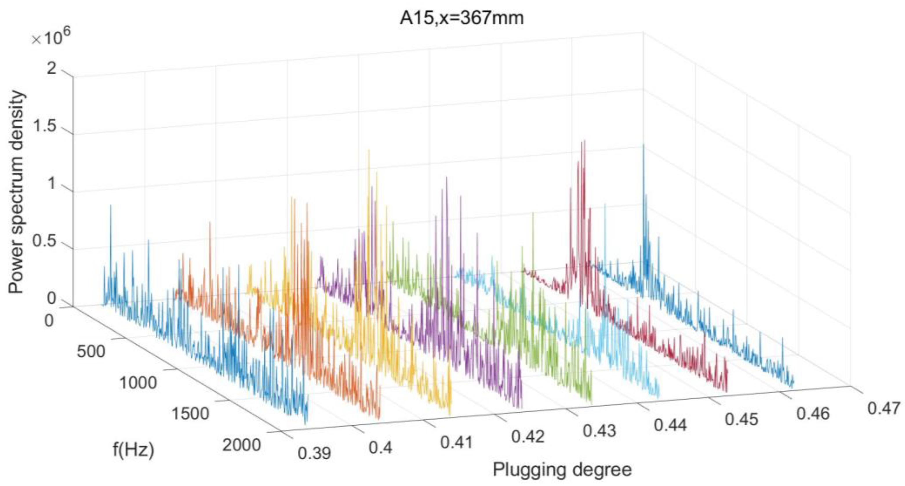
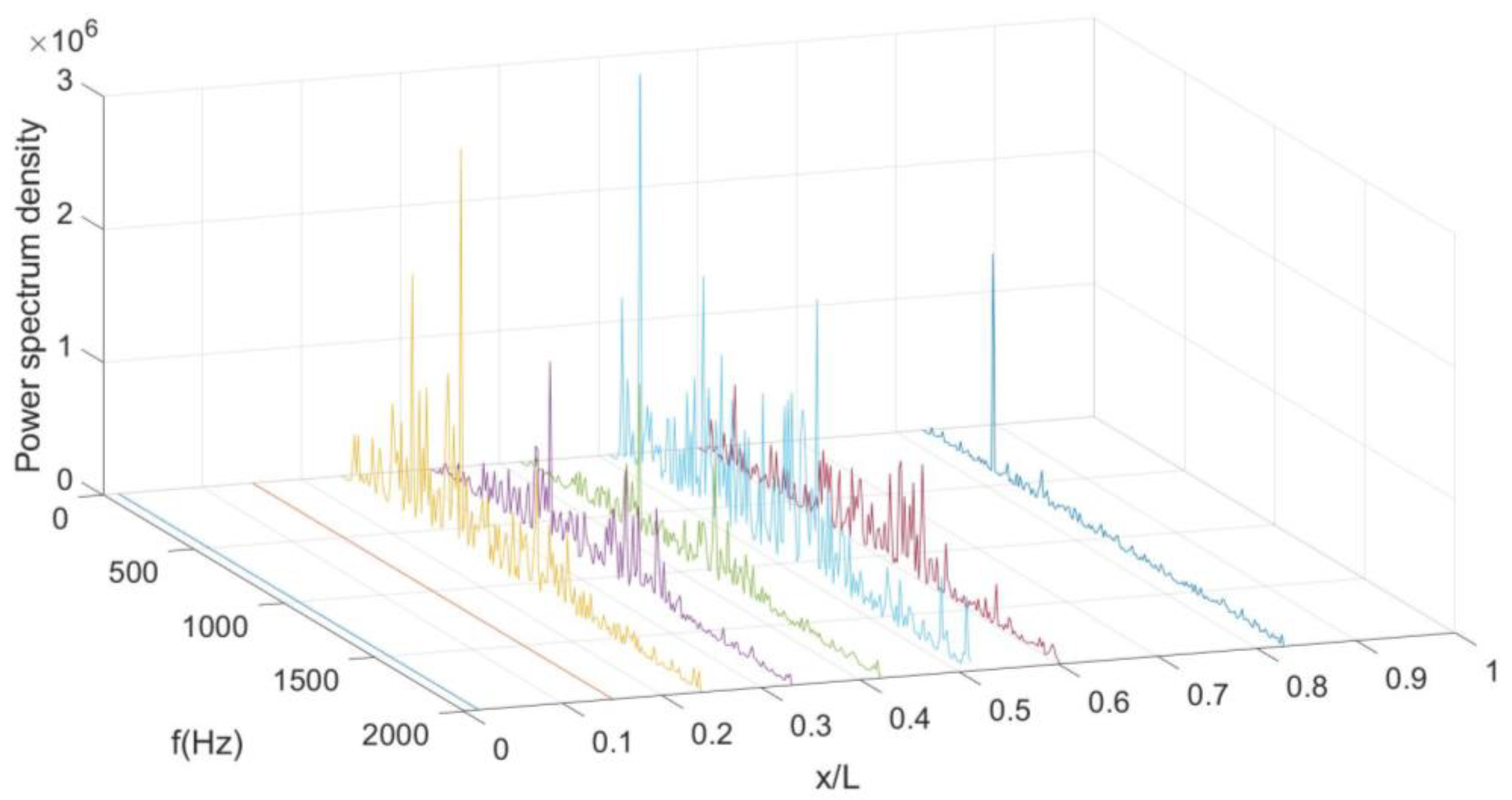
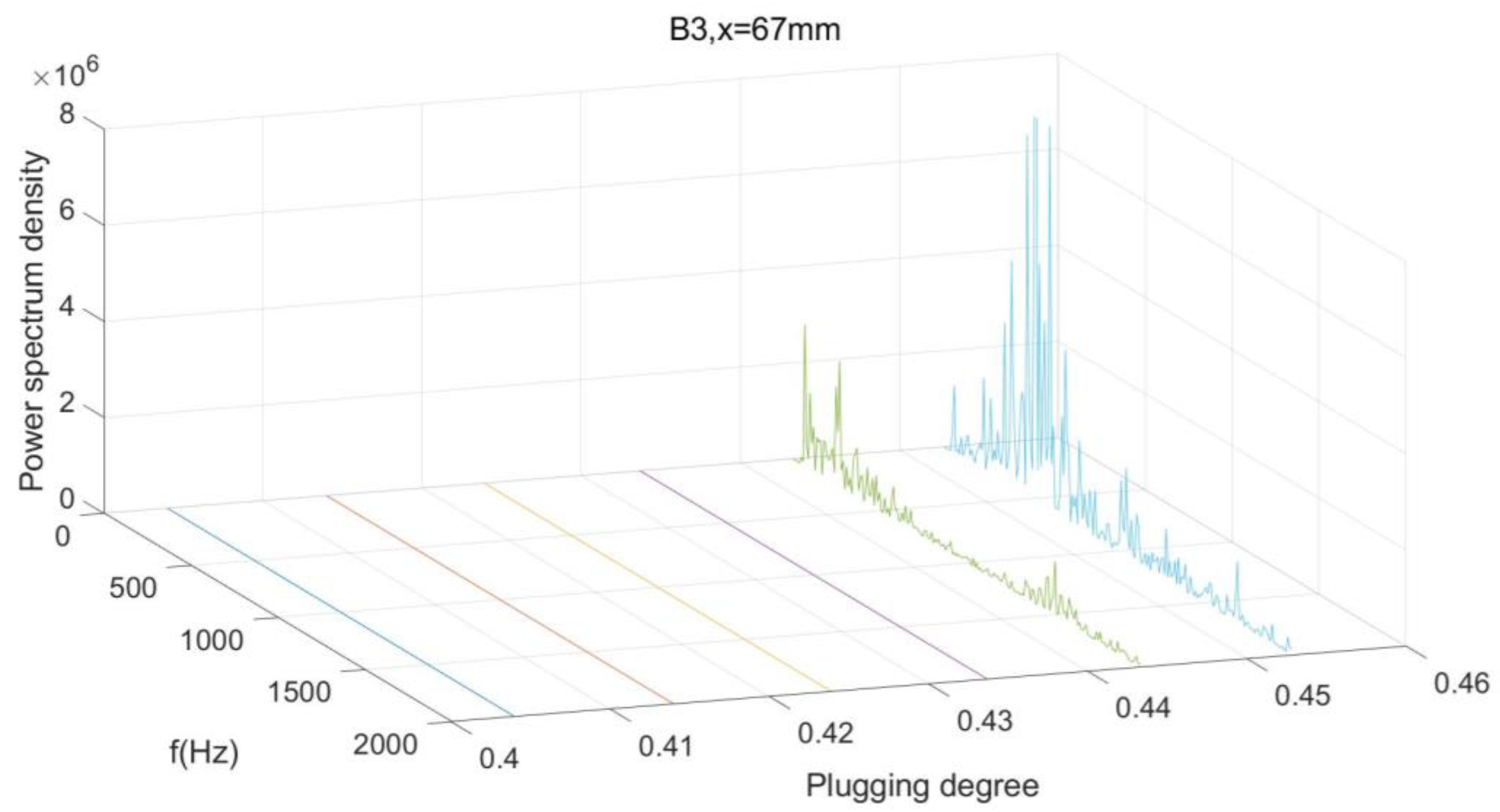
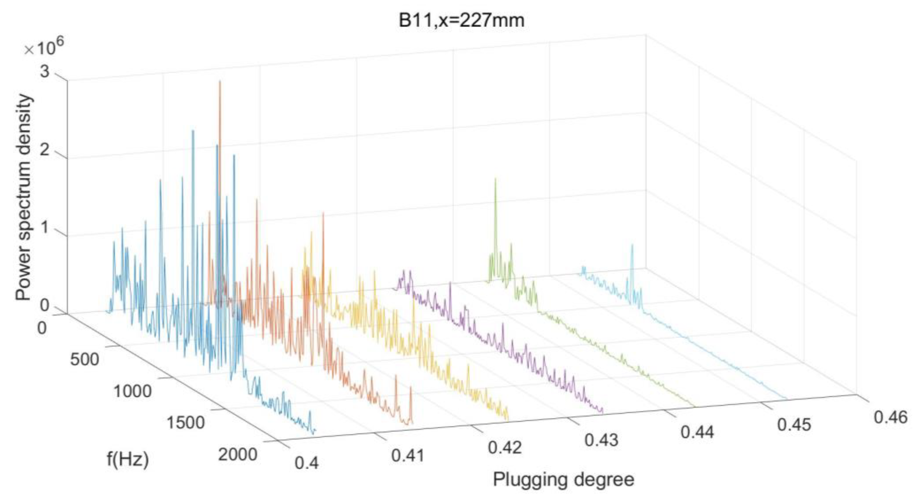
3.3. Power Spectrum Density Analyse of the Wall Pressure Oscillation

Figure 15 shows the results of the power spectrum density of the top wall sensor when the downstream plugging degree is 41.40%. Sensor A1 is located far upstream of the shock flow field, the pressure oscillation has no apparent main frequency, and the oscillation energy of all frequencies is low, which can almost be ignored. Sensor A3 is located at the shock train’s leading edge, and the pressure oscillation energy is relatively high. The energy of pressure oscillation is mainly concentrated at approximately 100 Hz and 500 Hz, and the overall energy of pressure oscillation is mainly concentrated at less than 1000 Hz. The energy of pressure oscillation at Sensor A5 is generally low, presumably because the sensor is located in the small separation zone behind the shock wave on the top wall. The energy of the oscillation within 100 Hz is deficient in A5 and downstream sensors, which is very high in sensors A1, and A3. Therefore, low-frequency oscillation does not easily propagate in the shock train flow field. The approximately 1300 Hz pressure oscillation energy of Sensor A7 is very high, which does not exist in the prior sensor because the sensor A7 is located near the point of the incident shock wave. The pressure oscillation energy of about 500 Hz and 1300 Hz of Sensors A9 and A11 is very high, indicating that high-frequency oscillations are easier to propagate in the shock train flow field.

The closer to the downstream of the shock train flow, the greater the energy loss due to shock loss and viscosity loss, so the pressure oscillation energy of sensor A15 is generally lower than sensor A11.

Figure 16 illustrates the power spectrum density results of each sensor on the lower wall when the downstream plugging degree is 41.40%. Sensor B1 is located far upstream of the shock train flow field. There is no apparent main pressure oscillation frequency, and all frequencies’ oscillation energy is low and nearly negligible. Sensor B3 is affected by the shock train flow field, and there is a certain pressure oscillation; however, the energy of the pressure oscillation is not high, demonstrating that the leading edge of the shock train will occasionally pass through this point when the shock train self-excites under this plugging degree condition. The pressure oscillation energy of Sensor B5 is relatively high, which reflects that the pressure oscillation at this point is relatively intense. The leading edge of the shock train continuously passes through this point under the condition of this plugging degree, causing severe pressure oscillation. The pressure oscillation energy at Sensor B7 is generally lower than that of the previous sensor, which is presumed to be because this point is in a small separation zone on the bottom wall. The pressure oscillation energy distribution of Sensors B9 and B11 is concentrated in the lower frequency band because the two sensors are in the large separation region of the bottom wall. Hence, the pressure oscillation frequency is low.

Notably, the energy distribution of pressure oscillations of Sensors A3 and B5 is very similar. Specifically, the frequency spectrum distribution of pressure oscillations in the intermittent region of the upper and lower walls is very similar, indicating that the oscillations of separated shock legs of bottom and top walls are mutually controlled, and the bifurcated shock waves oscillate as a whole, instead of two separate shock waves oscillating separately.

The overall pressure oscillation energy measured by sensor B15 is much lower than that of B11 for reasons similar to those analyzed above; sensor B15 is near the downstream of the shock train flow filed and has more viscous and shock loss energy than B11.

Figure 17 shows the power spectrum density image at the downstream plugging degree of pressure oscillation for 44.33%. With the increase in downstream congestion to 44.33%, sensor A1 has a specific pressure oscillation; the shock train flow field affected the sensor. Except for the last sensor, the pressure oscillation energy of other sensors is mainly distributed within 500 Hz, and the energy of the high-frequency band pressure oscillation was small. Figure 18 shows the power spectrum density image at the downstream plugging degree of pressure oscillation for 46.213%. As Figure 15 shows, the pressure oscillation at sensor A1 is more severe with a further increase in downstream congestion. Sensors A3 and A5 of pressure oscillation energy distribution were very similar, and the subsequent sensor’s shock wave streaming field pressure shock energy was generally low. In addition, in the S-shaped isolator, the shock train is not symmetric, a large separation zone may appear on the top wall or bottom wall, and the frequency of pressure oscillation in the large separation region is low.

In this paper, the “small” separation zone refers to the separation zone where a small separation occurs in the wall boundary layer in the shock train flow field. It then attaches later, and the “large” separation zone refers to the separation zone where a large separation occurs in the wall boundary layer and does not reattach but keeps developing and extending to the exit section, resulting in the low-speed zone of the exit section.

Under this plugging degree, the pressure oscillation energy of the sensor located downstream of the shock train is mainly concentrated below 500 Hz, such that the large separation zone of the shock train is located on the bottom wall.

Figure 19, Figure 20, Figure 21 and Figure 22 show the power spectrum density results of pressure oscillation sensors A3, A7, A11, and A15 under different downstream plugging degrees. The closer the sensor is downstream, the lower the downstream plugging degree corresponds to the first apparent pressure oscillation. In Sensors A7, A11, and A15, when the downstream plugging degree is more excellent than 44.33%, the energy of the pressure oscillation below 500 Hz rises suddenly, which is presumed to be because of the switch of the large separation region of the shock train from the bottom wall to the top wall, which causes the energy of low-frequency pressure oscillation to rise.

Figure 23 illustrates the power spectrum density image of pressure oscillation along the path measured by the bottom wall sensors when the downstream plugging degree is 41.40%. The pressure oscillation energy at Sensors B1 and B3 is low and negligible, demonstrating that the shock wave flow field does not affect this point. However, under the same plugging degree, the leading edge of the shock train reached Sensor A3 on the top wall, and the shape of the shock wave was not symmetric in the S-shaped isolator of the variable section. The leading edge of the shock train on the bottom wall was later than that on the top wall. At Sensor B5, the pressure oscillates violently. However, the pressure oscillations at Sensors B7 and B9 decreased because the two sensors were in the small separation zone behind the shock wave. Sensor B11 is located at the incident point of the shock wave. The shock leg continually sweeps over Sensor B11, and the pressure oscillation energy is high. Far downstream of the shock flow field, Sensor B15 is in the large separation zone at the exit of the bottom wall, and the pressure oscillation energy is low.

Figure 24 and Figure 25 show the power spectrum density images of pressure oscillation of downstream Sensor B3 and B11 under different downstream plugging degrees. For Sensor B3, when the plugging degree was 45.28%, the leading edge of the shock train reached the sensor. The value of Sensor A3 at the same x position was 41.40%. The pressure oscillation energy of the B11 sensor decreases gradually with the increase in the downstream plugging degree and the forward movement of the shock train.

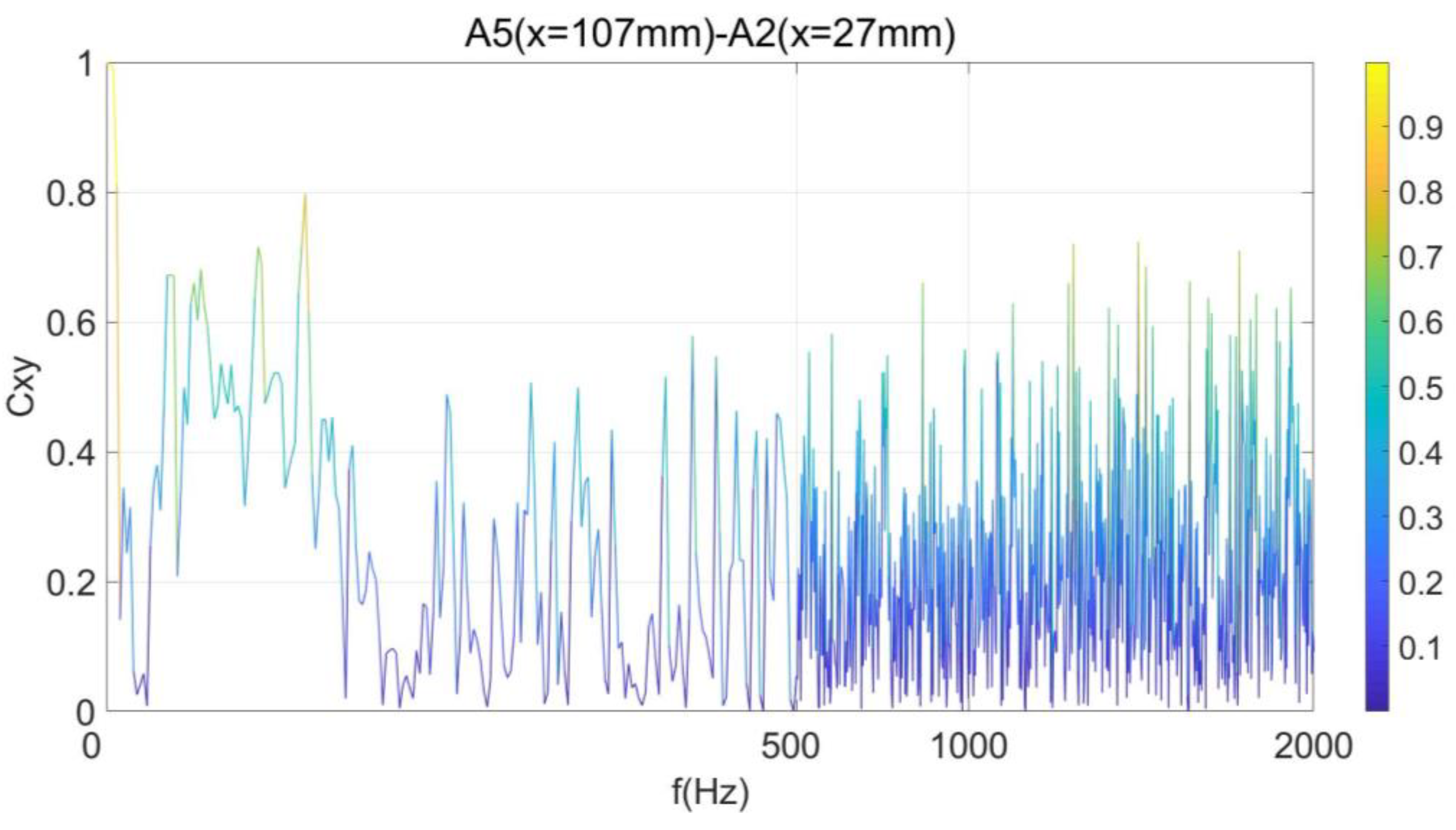
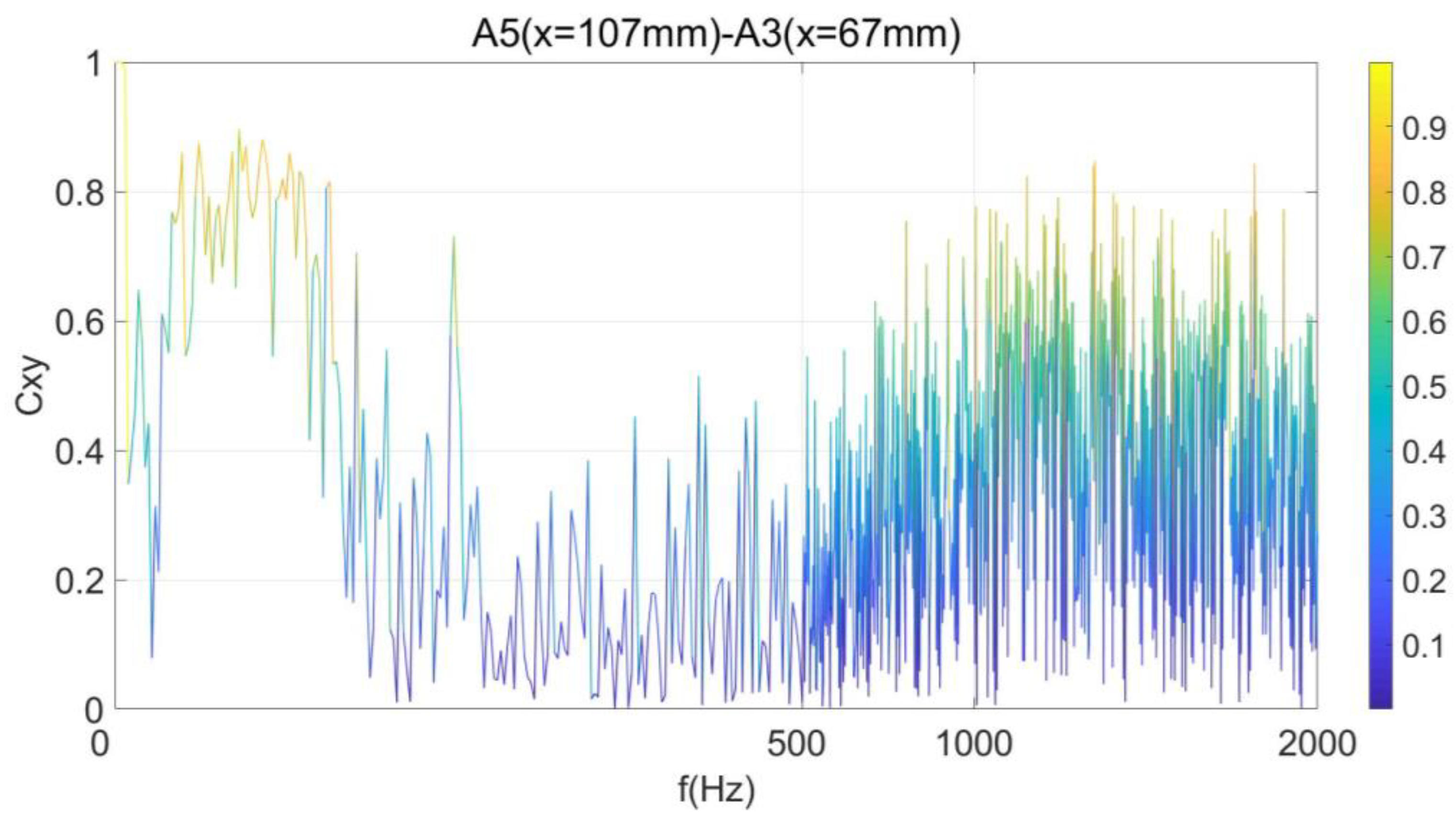
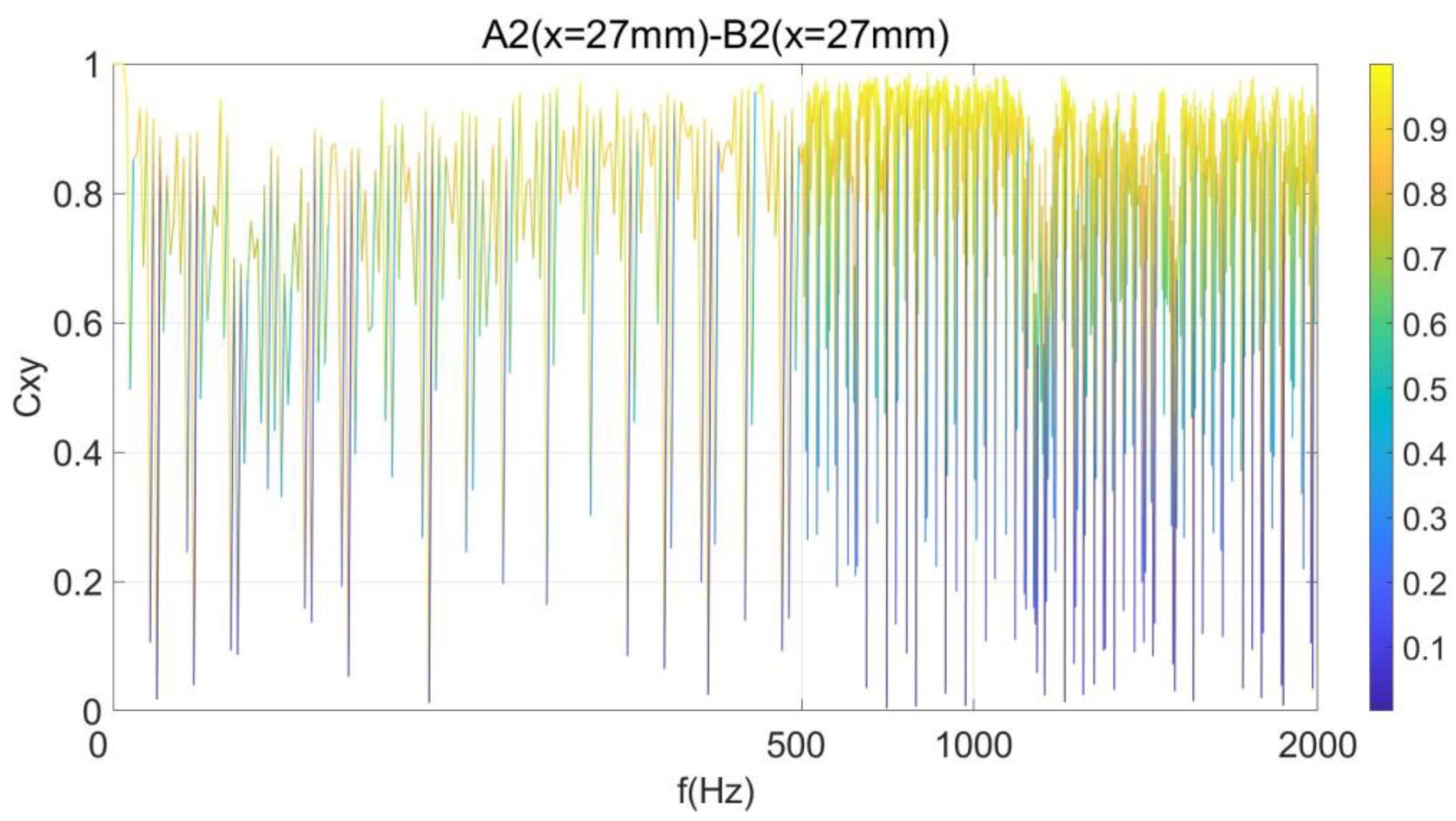
3.4. Analysis of Pressure Oscillation Coherence in the Shock Train Flow Field

To study the causality of the pressure oscillations at different measuring points, the coherence function was used in this subsection with two pressure signals, P_x(t) and P_y(t). The coherence function between them is defined as Equation (6):

$$C_{xy}\left(f\right)=\frac{{\left(P_{xy}\left(f\right)\right)}^2}{P_{xx}\left(f\right)P_{yy}\left(f\right)}$$

(6)

Figure 26, Figure 27 and Figure 28 illustrates the analysis results of the pressure oscillation coherence between Sensor A5 and Sensors A2, A3 and A4. The closer the distance between the two sensors, the stronger the coherence of the pressure oscillations within the 200 Hz frequency. In addition, Sensor A2 is located upstream of the shock train flow field, and Sensor A3 is located at the leading edge of the shock train. In terms of the correlation between pressure oscillations with a frequency below 200 Hz, Sensor A3 is significantly improved compared with Sensor A2. Therefore, the leading edge of the shock train can also be detected by analysing the coherence function between the measuring points in the isolator.

Figure 29 shows the plugging degree of 41.40% pressure oscillation on Sensors A2–B2 coherence analysis. The graph shows that the frequency of pressure oscillation coherence is very high because Sensors A2 and B2 were located in the flow of the turbulent boundary layer; the pressure characteristics were completely determined by the flow turbulence pulsation and were not affected by the separation shock train oscillation of the legs.

4. Conclusions

• The pressure oscillation in the area not affected by the shock train flow field is small and can be ignored. In the shock train flow field, the pressure oscillates most violently near the shock leg. The separation area exhibits low-pressure oscillation energy.
• The shape of the shock waves in the S-shaped isolator of the variable cross-section is asymmetrical, and the positions of shock legs on the upper and lower walls are inconsistent.
• The propagation speed of the shock train in the isolator of the variable section is not constant; however, it propagates slowly in the area involving rapid turning and quickly in the area involving gentle turning.
• It is difficult for the energy of a low-frequency oscillation to propagate from front to back in the shock flow field, while it is easier for the energy of a high-frequency oscillation. The frequency of oscillation is related to the local flow scale. The lower the pressure oscillation energy, the closer the oscillation is to the downstream region of the shock flow field.
• The boundary layer large separation mode of the shock wave flow field in the isolator section switches between the top and bottom walls, and the pressure oscillation frequency is low in the large separation area.

References

1. Waltrup, P.J.; Billig, F.S. Structure of shock waves in cylindrical ducts. AIAA J. 1973, 11, 1404–1408. [Google Scholar] [CrossRef]
2. Waltrup, P.J.; Dugger, G.L.; Billig, F.S. Direct-connect test of hydrogen-fueled supersonic combustion. Symp. Combust. 1977, 16, 1619–1629. [Google Scholar] [CrossRef]
3. Billig, F.S. Research on supersonic combustion. In Proceedings of the AIAA Aerospace Science Meeting, Reno, NV, USA, 6–9 January 1992. [Google Scholar]
4. Billig, F.S.; Dugger, G.L. The interaction of shock wave and heat addition in the design of supersonic combustors. Symp. Combust. 1969, 12, 1125–1139. [Google Scholar] [CrossRef]
5. Tian, X. Investigation of Flow in a Variable Cross-Section Isolator. Master’s Thesis, Nanjing University of Aeronautics and Astronautics, Nanjing, China, 2008. [Google Scholar]
6. Gao, L. Research on Isolators with Non-Constant Section and Complicated Condition. Master’s Thesis, Nanjing University of Aeronautics and Astronautics, Nanjing, China, 2011. [Google Scholar]
7. Tan, H.-J.; Guo, R.-W. Characteristics of Shock Train in Two Dimensional Bends with Constant Area. Acta Aeronaut. Astronaut. Sin. 2006, 27, 1039–1045. [Google Scholar]
8. Chen, J.-F.; Fan, X.-Q.; Meng, Z.; Xiong, B.; Wang, Y. Parameterization and Optimization for Variable Cross-Sections Bend Isolator. J. Propuls. Technol. 2020, 41, 1023–1030. [Google Scholar]
9. Wang, C.; Zhang, K.; Cheng, K. Effects of Incoming Flow Asymmetry on Shock Train Structures in Constant-Area Isolators. Trans. Nanjing Univ. Aeronaut. Astronaut. 2006, 23, 1–7. [Google Scholar]
10. Ding, M.; Li, H.; Fan, X.-Q. Numerical Simulation of Shock Train in a Constant Area Isolator. J. Natl. Univ. Def. Technol. 2001, 23, 15–18. [Google Scholar]
11. Wang, D.-P.; Zhao, W.-Z.; Sugiyama, H.; Tojo, A. Numerical and Experimental Investigations of Mach 4 Pseudo-Shock Waves in a Two-dimensional Square Duct. Acta Aeronaut. Astronaut. Sin. 2005, 26, 392–396. [Google Scholar]
12. Guo, S.; Wang, Z.; Zhao, Y. The flow hysteresis in the supersonic curved channel. J. Natl. Univ. Def. Technol. 2014, 36, 10–14. [Google Scholar]
13. Li, T. Study on Hysteresis Phenomenon Caused by Back Pressure in Curved Isolator. Master’s Thesis, National University of Defense Technology, Changsha, China, 2015. [Google Scholar]
14. Zhang, H. Characteristics of Shock-Train at Complicated Geometrical and Incoming Flow Conditions. Master’s Thesis, Nanjing University of Aeronautics and Astronautics, Nanjing, China, 2009. [Google Scholar]
15. Xiong, B.; Fan, X.-Q.; Wang, Z. Oscillation characteristics of shock train in deflected center-line isolator. J. Aerosp. Power 2016, 30, 1669–1675. [Google Scholar]
16. Xiong, B.; Fan, X.-Q.; Tao, Y.; Li, T. Influence of deflected center-line on performance of isolator. J. Rocket Propuls. 2016, 42, 35–41. [Google Scholar]
17. Huang, H.; Tan, H.; Sun, S.; Wang, Z. Behavior of shock train in curved isolators with complex background waves. AIAA J. 2018, 56, 329–341. [Google Scholar] [CrossRef]
18. An, B.; Fan, X.-Q.; Li, T.; Xiong, B. Numerical investigation on characteristics of shock train in S-shaped isolation section in scramjet engine. J. Rocket Propuls. 2016, 42, 47–52. [Google Scholar]
19. Tan, H.; Sun, S. Preliminary Study of Shock Train in a Curved Variable-Section Diffuser. J. Propuls. Power 2008, 24, 245–252. [Google Scholar] [CrossRef]
20. Kawatsu, K.; Koike, S.; Kumasaka, T.; Masuya, G.; Takita, K. Pseudo-Shock Wave Produced by Backpressure in Straight and DivergingRectangular Ducts. In Proceedings of the AIAA/CIRA 13th International Space Planes and Hypersonics Systems and Technologies, Sendai, Japan, 20–24 June 2005. [Google Scholar]
Figure 1. The results of the verification of the numerical calculation method.
Aerospace 10 00002 g001
Figure 2. Schematic diagram of the experimental bench.
Aerospace 10 00002 g002
Figure 3. Throttle device physical diagram and structure diagram.
Aerospace 10 00002 g003
Figure 4. Transversal dimensions of the channel cross-section.
Aerospace 10 00002 g004
Figure 5. Schematic diagram of the isolator.
Aerospace 10 00002 g005
Figure 6. Comparison of the experiments and simulations without back pressure.
Aerospace 10 00002 g006
Figure 7. Comparison of the experiments and simulations with back pressure at Pb/P1 = 3.
Aerospace 10 00002 g007
Figure 8. Dimensionless pressure–timing curves of Sensors A1, A3, A5 and A7 under 41.40% downstream plugging degree.
Aerospace 10 00002 g008
Figure 9. Dimensionless pressure–timing curves of Sensors B2, B4 and B6 under 41.40% downstream plugging degree.
Aerospace 10 00002 g009
Figure 10. Dimensionless pressure oscillation curves of Sensor A3 at plugging degrees of 39.39%, 41.40% and 43.37%.
Aerospace 10 00002 g010
Figure 11. Mach number cloud image of symmetric plane of isolator section under different backpressure conditions.
Aerospace 10 00002 g011
Figure 12. Dimensionless pressure oscillation curve of the pressure sensor when the back pressure is slowly applied.
Aerospace 10 00002 g012
Figure 13. Definition of the intermittent rate.
Aerospace 10 00002 g013
Figure 14. Curves of sensor intermittent rate changing with time.
Aerospace 10 00002 g014
Figure 15. Power spectrum density and accumulative frequency of the top wall sensor when the downstream plugging degree is 41.40%.
Aerospace 10 00002 g015
Figure 16. Power spectrum density and the accumulative frequency of the bottom wall sensor when the downstream plugging degree is 41.40%.
Aerospace 10 00002 g016aAerospace 10 00002 g016b
Figure 17. Power spectrum density of the top wall sensor when the downstream plugging degree is 44.33%.
Aerospace 10 00002 g017
Figure 18. Power spectrum density of the top wall sensor when the downstream plugging degree is 46.21%.
Aerospace 10 00002 g018
Figure 19. Power spectrum density results of pressure oscillation of Sensor A3 under different downstream plugging degrees.
Aerospace 10 00002 g019
Figure 20. Power spectrum density results of pressure oscillation of Sensor A7 under different downstream plugging degrees.
Aerospace 10 00002 g020
Figure 21. Power spectrum density results of pressure oscillation of Sensor A11 under different downstream plugging degrees.
Aerospace 10 00002 g021
Figure 22. Power spectrum density results of pressure oscillation of Sensor A15 under different downstream plugging degrees.
Aerospace 10 00002 g022
Figure 23. Power spectrum density of the bottom wall sensors when the downstream plugging degree is 41.40%.
Aerospace 10 00002 g023
Figure 24. Power spectrum density results of pressure oscillation of Sensor B3 under different downstream plugging degrees.
Aerospace 10 00002 g024
Figure 25. Power spectrum density results of pressure oscillation of Sensor B11 under different downstream plugging degrees.
Aerospace 10 00002 g025
Figure 26. Pressure oscillation correlation of Sensors A2 and A5.
Aerospace 10 00002 g026
Figure 27. Pressure oscillation correlation of Sensors A3 and A5.
Aerospace 10 00002 g027
Figure 28. Pressure oscillation correlation of Sensors A4 and A5.
Aerospace 10 00002 g028
Figure 29. Pressure oscillation correlation of Sensors A2 and B2.
Aerospace 10 00002 g029