Predicting Water Availability in Water Bodies under the Influence of Precipitation and Water Management Actions Using VAR/VECM/LSTM

Abstract

Recently, awareness about the significance of water management has risen as population growth and global warming increase, and economic activities and land use continue to stress our water resources. In addition, global water sustenance efforts are crippled by capital-intensive water treatments and water reclamation projects. In this paper, a study of water bodies to predict the amount of water in each water body using identifiable unique features and to assess the behavior of these features on others in the event of shock was undertaken. A comparative study, using a parametric model, was conducted among Vector Autoregression (VAR), the Vector Error Correction Model (VECM), and the Long Short-Term Memory (LSTM) model for determining the change in water level and water flow of water bodies. Besides, orthogonalized impulse responses (OIR) and forecast error variance decompositions (FEVD) explaining the evolution of water levels and flow rates, the study shows the significance of VAR/VECM models over LSTM. It was found that on some water bodies, the VAR model gave reliable results. In contrast, water bodies such as water springs gave mixed results of VAR/VECM.

1. Introduction

Water is the most critical resource for life. With a country’s increasing population, an increase in water demand is expected [1]. According to the United Nations’ projection, a large number of people (4.5 billion people) may be influenced by a water crisis by 2050. Increasing population will increase food demand, and more water will be required for crop irrigation [1,2]. Climate change is expected to affect available water resources significantly (e.g., affecting groundwater recharging) [3]. Climate change and/or variability directly impact groundwater systems through replenishment by recharge and indirectly through changes in groundwater usage [4]. Given all these situations, different water bodies have been analyzed to predict their water level or flow rate. In this paper, nine datasets from different regions of Italy were used for investigation, to predict water levels and flows. Datasets contain various rainfalls or temperatures, flow rates from water springs, hydrometric data from rivers, or lakes, and groundwater levels. The U.S. Geological Survey has a web page describing the water cycle, giving insight into the performance of feature engineering. For example, much of the water in rivers and lakes comes from surface runoff (influenced by the type and saturation of the soil). Water enters aquifers in form of precipitation and penetrates slowly through the soil, therefore took longer time to resurface the water level through springs and wells [5,6]. How these variables act together can be understood through a series of events—the weather is the exogenous force. Rain pours down and collects into rivers from where it fills lakes and later reaches aquifers, depending on the permeability of the soil. These water bodies may exercise pressure on each other, causing water springs to change. Climate change can also result in a change in the rate of precipitation patterns. The order of these events is essential to define the causal relationships. This paper mainly addressed the issues of water bodies by predicting the amount of water in each water body using identifiable unique features and assessing the behavior of these features on others in the event of a shock. Each water body is unique and has different features and variables that can influence water availability over time; therefore, we need to predict the essential variables. In the above discussion, we found that these water bodies (aquifers, water springs, lakes, rivers) are connected to each other and affect the overall water availability. To access real available water, precise estimation of water availability from these water bodies is necessary. Therefore, in this study, the available water in all these water bodies is estimated using different prediction models.

The models used have some limitations: VAR and VECM serve as linear predictors. To capture nonlinear behavior of water bodies, Long Short-Term Memory (LSTM) is utilized in this study. However, LSTM is sensitive to initial hidden states. It requires large datasets to be trained to precision [7]. Therefore, the reasons for choosing our models are as follows: The VAR and VECM models can be expected to be least biased due to their linear properties—possibly at the cost of a higher RMSE/MAE. Contrary to complex machine learning models, our models allow for the investigation of causal relationships. The low bias in our models enables reliable interpretations of the OIR plots, which are helpful to determine causal relationships between features—such tools are not available for black-box models.

2. Related Works

Traditionally, hydrological models were constructed using domain experts in most of the water resource system research. Models constructed usually describe the relations between variables using predefined formulas.

Many data-driven models have been employed to improve water demand (WD) forecasting, recognizing the bias in a simple linear regression model [8]. Autoregressive (AR) data-driven methods—analysis of a time series is utilized for analyzing historical data—have been commonly employed in the relevant literature [9]. Literature has demonstrated that AR methods, such as the autoregressive integrated moving average (ARIMA), perform better than classical linear regression approaches in forecasting short-term urban WDs and runoff [9,10].

Researchers have considered the VAR model with different orders for multivariate time series models and ARIMA models for univariate time series models [11,12,13]. Multivariate time series analysis (MVTSA) introduces a way to observe the relationship of a group of variables over time [14], thus making use of all possible information such as correlation [15].

The main idea behind time series forecasting is to create an insight into the system of the underlying measurement session. In the last two decades, machine learning methods have captivated hydrological research interest. Time series models are non-parametric and data-driven, aiming to improve a prediction task [16]. They use past information for training data and utilize stochastic dependencies to accomplish their goal in the underlying structure. The combination of knowledge from both statistics and computing science leads to varying models and specifications. Noisy data, missing labeled data, irrelevant or imbalanced data, and circumscribed model interpretability raise challenging issues in machine learning solutions [17,18].

Recurrent Neural Networks (RNNs) consider network output of previous time steps in later iterations for processing sequential data. Learning long-term and short-term dependencies without losing efficiency is a challenging problem that many researchers have encountered, resulting in specialized and generalized models. Groenen et al. [19] compared RNN architecture and implemented seasonality extraction, residual learning, and accurately predicting wastewater influx at municipal wastewater treatment plants. Bontsema et al. [20] also did a comparative study on wastewater effluent quality focusing on regression trees. Traditional feature construction might surmount LSTMs for multivariate time series [20].

An LSTM is a special RNN that can memorize previous information and calculate the current output [21]. Lecun et al. [22] explained that it is suitable for processing water quality time series data due to its long-term memory capability. It can also solve the problems of gradient disappearance in standard RNN by selectively forgetting or memorizing some data [18].

Many recent publications exist related to the water sector in which LSTMs are used. In the study of Xiang et al. [23], the authors developed a rainfall-runoff model; in their study, Elsheikh et al. [24] used LSTMs to forecast water production in solar stills; Barzegar et al. [25] performed a short-term water quality variable prediction whereas Xu et al. [26] used LSTMs to detect abnormal working conditions in water supply networks. Two approaches are generalized here in forecasting multiple subsequent observations of a time series. Recursive forecasting, also known as the iterative forecasting model, iteratively produces a prediction for a single interval ahead, using a fixed slot of past information/data and predictions of past information/data if their actual values are not given. At the same time, direct forecasting produces a prediction for multiple time intervals ahead independent of the information/data in between. Conventionally, statistical time series methods such as VAR lie under the category of recursive forecasting. They can be customized to produce a forecast for multiple intervals ahead. McCraken et al. [27] talk about VAR models in detail, focusing on their utilization in direct and recursive forecasting. Further in his paper, McCraken demonstrated a comparison of two methods for conditional forecasting and concluded that the recursive method acts better than the direct method [27].

In the study of Zhao et al. [28], the VAR method describes the long-term influence of soil and water conservation measurements on runoff, reflecting distinct effects of different soil conservation measurements and different stages of the exact measurements on runoff. Yoke et al. [29] found the VAR model suitable for modeling rainfall and ground level; a one-way causality between rainfall and groundwater level is reported using the Granger causality. Hartini et al. [30] discussed the significant relationships between river discharge and rainfall, indicating that the study area moved downstream.

Pradhan et al. [31] used the Vector Error Correction Model (VECM) to find bidirectional causality between road transportation and economic growth. In a much recent publication, VECM is used to build similar models. A similar model for a market, taking into account the electricity, coal, gas, and carbon prices as endogenous parameters, was developed by Honkatukia et al. [32]. Fell et al. [33] used the same market dataset and, considering the same prices, adding the water level of the reservoir and the temperature as exogenous regressor to the VECM. Chemarin et al. [34] focused on climatic conditions and considered two climatic parameters: temperature, having an impact on the demand side of the electricity market, and rainfall influencing the electricity-producing capacity of a country concerning its energy mix, for estimating a VECM for the French power market [34]. A similar econometric approach followed in the paper of Thoenes et al. [35], who investigated the relationships among the prices of fuels, electricity, and carbon for the German market [35].

The VAR method is utilized when the used data have stationarity at a level; when the study data have not stationarity at a level but if they are stationary at the first difference value, then the Autoregressive Vector in Difference (VARD) utilizes variables that do not have cointegration. Suppose the studied parameters have stationarity and cointegration at the first difference value. In that case, the Vector Error Correction Model (VECM) is utilized. VECM modeling is used for multivariate time series data, which will then detect the causal relationship between variables using Granger Causality to visualize the effect of variable variability compared to other variables using the Impulse Response Function (IRF) [36].

3. Methodology Used

3.1. Vector Autoregressive (VAR)

VAR is a simultaneous equation, which can be implemented on stationary variables. If variables have no stationarity, we use the Vector Error Correction Model (VECM), with the condition applied. One or more cointegration relations exist between the used variables. VECM is a version of VAR meant to be utilized for known existing cointegration relationships for non-stationary [37].

$$y_t={\displaystyle \sum }_{i=1}^p{A}_i{y}_{t-i}+{\epsilon }_t$$

(1)

where, γ_t: is the vector of observation, A: parameter matrix, ε_t: a vector of error, _t: is at any instant of time.

Suppose the differencing level and cointegration are the same, where the data is stationary. In that case, the VAR and the error correction model are combined to provide the Vector Error Correction Model (VECM) [38].

3.2. Vector Error Correction Model (VECM)

VECM is a version of VAR intended to be utilized in a time series having non-stationarity and a cointegration relationship between the variables. VECM can predict the short-term impacts between variables and the long-term impacts of time series data. A generalized VECM (p), where p represents the lag of endogenous variables with cointegration rank r ≤ k, can be expressed [39]:

$$\Delta y_t={{\displaystyle \prod }}^{}{y}_{t-1}+{\displaystyle \sum }_{i=1}^{p-1}{\mathsf{\Gamma }}_i\Delta y_{t-i}+D_t+{\phi }_t$$

(2)

where: ∆ = operator differencing, where ∆γ_t = γ_t − γ_t−1, y_t−1 = vector variable endogenous with lag1, ${\phi }_t$ = k × 1 vector residuals, D_t = k × 1 vector constant, Π = matrix coefficient of cointegration (Π = αβ^t; α = vector adjustment, k × r matrix and β = matrix cointegration (long-run parameter) (k × r)) Γ_i = k × k matrix coefficient the i th variable endogenous. p represents the lag; r is the cointegration rank; k is the size of vectors considered.

3.3. Long Short Term Memory (LSTM)

LSTM comprises a complex structure, the LSTM cell in its middle layer. In Figure 1, we can see the LSTM cell comprises three gates; input, forget, and output gates, which have control over the flow of information across the cell and the neural network (NN).Input variable $x_t$ is at any instant t, $h_t$ is the hidden layer output and $h_{t-1}$ is its former output, Ĉ_t represents the cell input state, the cell output state is given as $C_t$, and $C_{t-1}$ is its former state, $i_t$, $f_t$, and $o_t$ are the three gate’s states. Both $C_t$ and $h_t$ are transmitted to the following NN in RNN, determined by the structure of the LSTM cell. We use Equation (3) in order to evaluate $C_t$ and $h_t$.

After evaluating the three gate’s states, proceed to the cell input state,

$$i_t=\sigma \left(W_1^i.x_t+W_h^i.h_{t-1}+b_i\right),$$

(3)

forget gate:

$$f_t=\sigma \left(W_1^f.x_t+W_h^f.h_{t-1}+b_f\right)$$

(4)

output gate:

$$o_t=\sigma \left(W_1^o.x_t+W_h^o.h_{t-1}+b_o\right)$$

(5)

cell input:

$${Ĉ}_t=tanh\left(W_1^C.x_t+W_h^C.h_{t-1}+b_C\right)$$

(6)

where weight matrics ($W_1^i$, $W_1^f$, $W_1^o$, $W_1^C$) connects x_t to the three gates and the cell input, weight metrics $W_h^i$, $W_h^f$, $W_h^o$, $W_h^C$ connects h_t−1 to the three gates and cell input, bias terms for all three gates and cell inputs (b_i, b_f, b_o, b_C), the sigmoid function ($\frac{1}{1+\exp \left(-x\right)}$) given by σ and the hyperbolic tangent function, ($\frac{\exp \left(x\right)-\exp \left(-x\right)}{\exp \left(x\right)+\exp \left(-x\right)}$), represented by tanh.

Now we evaluate the cell output state:

$$C_t=i_t\ast {Ĉ}_t+f_t\ast C_{t-1}$$

(7)

where i_t, f_t, $Ĉ$_t, C_t−1, and C_t have the same dimensions.

Finally, we evaluate the hidden layer output [40]:

$$h_t=o_t\ast \tan \mathrm{h}\left(C_t\right)$$

(8)

4. Evaluation Metrics

4.1. Mean Absolute Error (MAE)

MAE is the average magnitude of error in a set of predictions that can be measured using MAE without considering their direction. The MAE value is obtained by calculating the average over the absolute differences between the predicted and observed values. Every difference has the same weight.

$$MAE=\frac{1}{n}{\displaystyle \sum }_{j=1}^n\left|y_j-{\widehat{y}}_j\right|$$

(9)

n: no. of observed value, y_j: observed value.

4.2. Root Mean Squared Error (RMSE)

RMSE is the average magnitude of error that can be measured using RMSE by calculating the square root of the average squared differences between predicted and observed values.

$$RMSE=\sqrt{\frac{1}{n}{\displaystyle \sum }_{j=1}^n{\left(y_j-{\widehat{y}}_j\right)}^2}$$

(10)

n: no. of observed values, y_j: observed value.

RMSE and MAE both give an average error for the prediction model in units for the considered variables. Both can give values in the range of 0 to infinity. Lower values give better results, and both are insensitive to the direction of errors. RMSE gives a relatively high weight to significant errors, as errors are squared and averaged. It is directly proportional to the variance of the frequency distribution of errors [41]. RMSE is adopted in this study due to successful application of this statistical index in the literature [42,43,44,45,46].

4.3. Model Framework

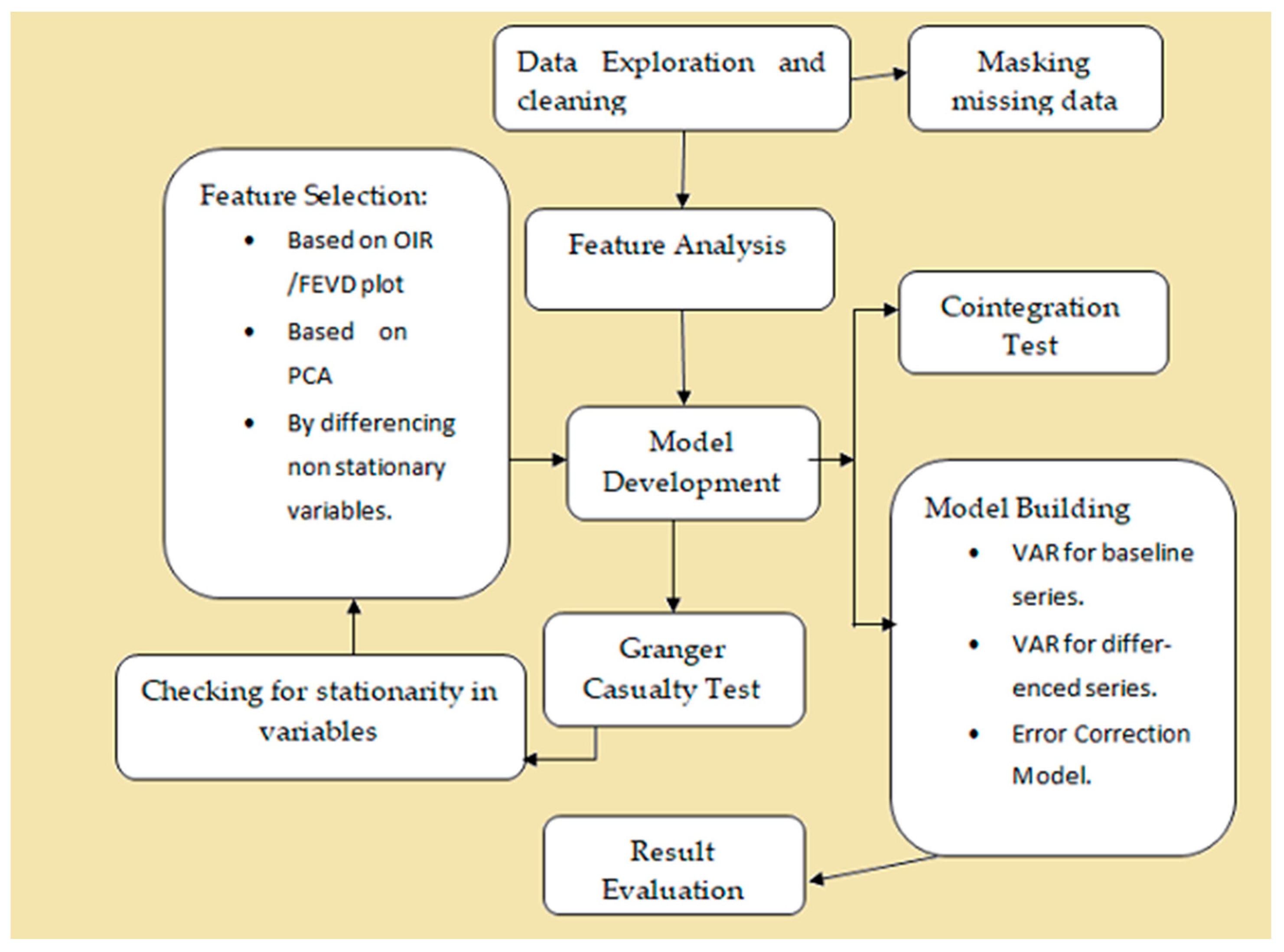
We construct a time series model for each water body category, i.e., aquifers, water springs, lakes, and rivers. In this way, it is possible to optimize every phase for every category to obtain the best result. In particular, the different phases developed are discussed here, and the whole workflow is shown in Figure 2:

Initially, data are explored to understand their variables and their distribution, followed by an analysis of missing data, which is resolved by masking or imputing as per requirement. Outliers will be detected using the Z-score method and will be set as NaN. The Z-score determines how many standard deviations away a data point is from the mean.

Figure 3 shows the distribution of the Petrignano-aquifer. The distribution shown in Figure 3 is plotted after the data cleaning process. The rolling average also seems beneficial in smoothing out some noise from features, and can avoid overfitting.

In a subsequent phase, we will make a feature selection, and feature selection approaches are listed below:

The Orthogonalized Impulse Response (OIR) plot, analyzes shock occurring in one variable at a time. It captures the contemporaneous correlation of error terms, as it relies on stronger assumptions. Thus, the order of features in the model matters. The OIR plot illustrates (orthogonalized) feature shocks which contribute to the error variance of our target features in different lags.

Principal Component Analysis (PCA), uses linear algebra to transform the dataset into a compressed form. Generally, this is called a data reduction technique. While using PCA, one can choose the desired number of dimensions or principal components in the transformed result.They are different non-static variables.

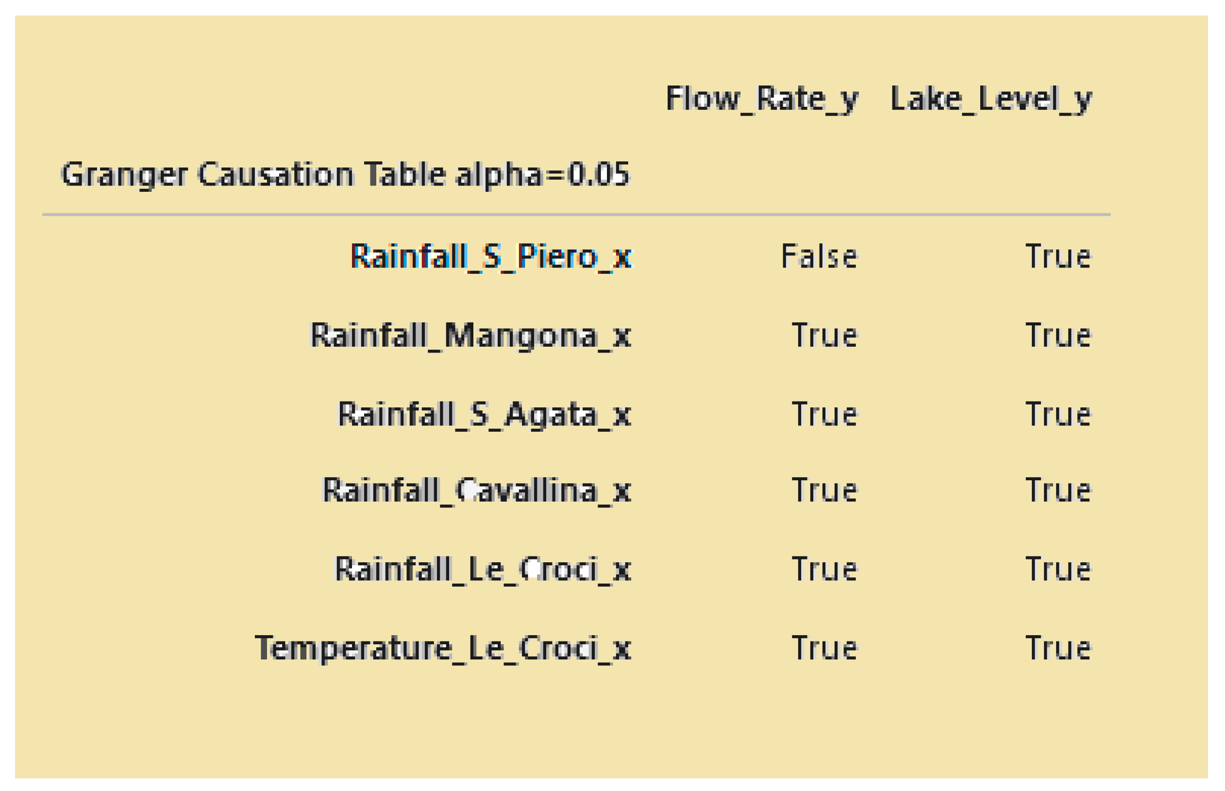
For model development, the datasets are divided into three categories: training set (80%), testing set (10%), validation set (10%). A training set is used to build a baseline VAR model which includes all the significant features, then by analysis of the OIR plot significant features are picked. We conducted the Granger Causality test to depict the relationship between choosing features and target variables, as shown in Figure 4; for further reducing features. If features are not stationary, they can be made stationary by a differencing method; likewise, different features can be used to train the model. After comparing all models, the best model is used to compare with LSTM as in

Table 1. Summary of Depth of Groundwater (aquifers).

Aquifer		VAR			LSTM
	Steps	RMSE (m)	MAE (m)		RMSE (m)	MAE (m)
Auser	1-day	0.0516	0.0374	Before scaling	0.1516	0.1129
	7-day	0.0457	0.0389	After scaling	0.2089	0.1640
	14-day	0.0583	0.0490
Doganella	1-day	0.6030	0.1732	Before scaling	0.3875	0.2525
	7-day	0.1540	0.1255	After scaling	1.7477	1.3480
	14-day	0.2257	0.1912
Luco	1-day	0.466	0.0311	Before scaling	0.0843	0.0647
	7-day	0.0577	0.0430	After scaling	0.0464	0.0356
	14-day	0.0394	0.0264
Petrignano	1-day	0.1004	0.0729	Before scaling	0.0319	0.0256
	7-day	0.2999	0.2919	After scaling	0.2346	0.1884
	14-day	0.2709	0.2276

,

Table 2. Summary of Flow Rate (lake).

Lake	Steps	VAR			LSTM
		RMSE (m/s)	MAE (m/s)		RMSE (m/s)	MAE (m/s)
Blancino	1-day	0.8862	0.3404	Before scaling	0.0585	0.0388
	7-day	0.1205	0.1096	After scaling	1.1897	0.7056
	14-day	0.1081	0.0894

,

Table 3. Summary of Water Level (river).

River	Steps	VAR			LSTM
		RMSE (m)	MAE (m)		RMSE (m)	MAE (m)
Arno	1-day	0.1172	0.0731	Before scaling	0.0582	0.0436
	7-day	0.0486	0.0441	After scaling	0.1358	0.1017
	14-day	0.0686	0.0657

and

Table 4. Summary of Flow rate (water springs).

Water Spring		Steps	VAR		VECM
			RMSE (m/s)	MAE (m/s)	RMSE (m/s)	MAE (m/s)
Amiata	Flow_Rate_Bugnano	1-day	0.0383	0.0304	0.0112	0.007
		7-day	0.0306	0.0274	0.0138	0.010
		14-day	0.0253	0.0238	0.0153	0.012
	Flow_Rate_Arbure	1-day	0.0222	0.0157	0.0825	0.0546
		7-day	0.0506	0.0422	0.0904	0.676
		14-day	0.0952	0.0889	0.0938	0.075
	Flow_Rate_Ermicciolo	1-day	0.3136	0.2942	0.1591	0.1221
		7-day	0.1779	0.1477	0.1907	0.1538
		14-day	0.0966	0.0845	0.2092	0.1726
	Flow_Rate_Gallaria_Alta	1-day	0.1971	0.1264	0.6151	0.4048
		7-day	0.4927	0.3748	0.727	0.5307
		14-day	0.8950	0.8185	0.7609	0.6057
Lupa	Flow_rate_Lupa	1-day	0.4206	0.0944	0.4233	0.0941
		7-day	1.4715	0.5708	1.4715	0.5699
		14-day	2.4280	1.2444	2.4270	1.2439
Madonna-Di-Canetto	Flow_rate_Madonna-di-canneto	1-day	9.5089	5.396	11.6846	6.4348
		7-day	14.0742	10.3333	12.8215	8.9599
		14-day	13.0118	10.9436	12.0066	9.6939

.

In some instances, the time-series variable shows many lags, indicating that a long-memory process may improve performance. This means that a shock may lead to a relatively persistent change in the water flow. A VECM model could capture this memory.

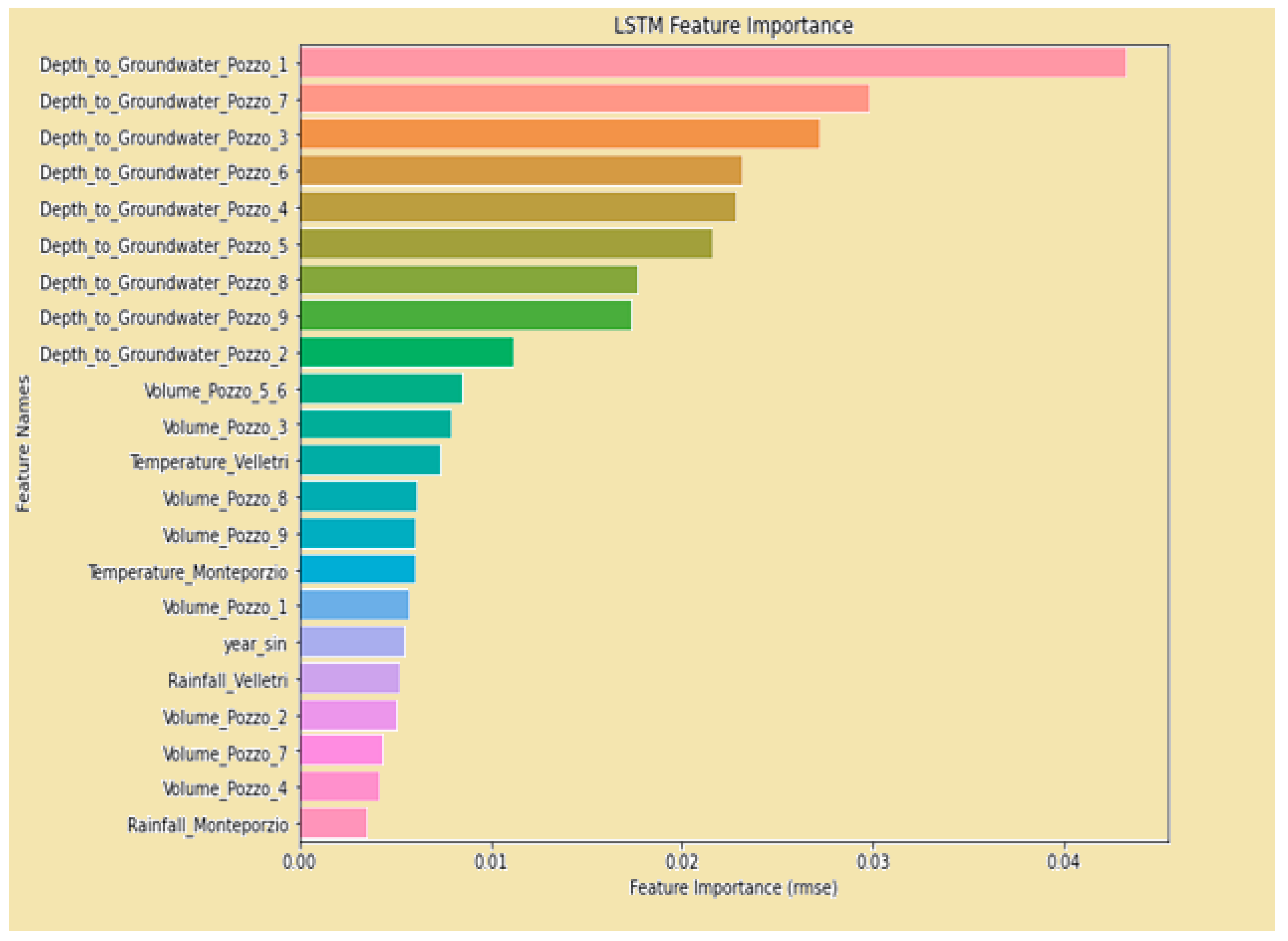
The LSTM model used in this paper required scaled data; therefore, we first scaled our data using normalization procedure. We use the same lag as VAR to train the LSTM for a single-day prediction performance comparison. The model focuses only on the feature importance learned by the LSTM. We use the sensitivity analysis to determine the feature importance (an example is shown in Figure 5). When perturbing a particular feature based on testing data, given the values of the other feature remain unchanged, the behavior of RMSE is emphasized by comparing the prediction before and after perturbation. The feature is found more significant if the value of RMSE estimated is considerably more than other features.

The Durbin–Watson test and the Portmanteau test were performed to verify the quality of the time series models used. While the Durbin–Watson test checks if the error terms are autocorrelated at a lag order of one, the Portmanteau test checks if the autocorrelation of several lags is zero. We always chose the number of lags to be a multiple of the respective model. Usually, we found that there was still autocorrelation left in the error terms. We also checked with a test for normality (Jarque–Bera test) of the error terms, which was denied in all cases. Failing to pass the normality test means that asymptotic standard errors are no longer valid. Bootstrapping methods such as Efron’s or Hall’s confidence interval should be used instead of checking the impulse response. For the VECM, since it detects cointegration relations among features and thus does not require stationary data, we used the Johansen cointegration test to help to select the cointegration rank. Finally, OIR/FEVD analysis of VAR and sensitivity analysis of LSTM are reported to gain insight into feature importance.

5. Case Study Area

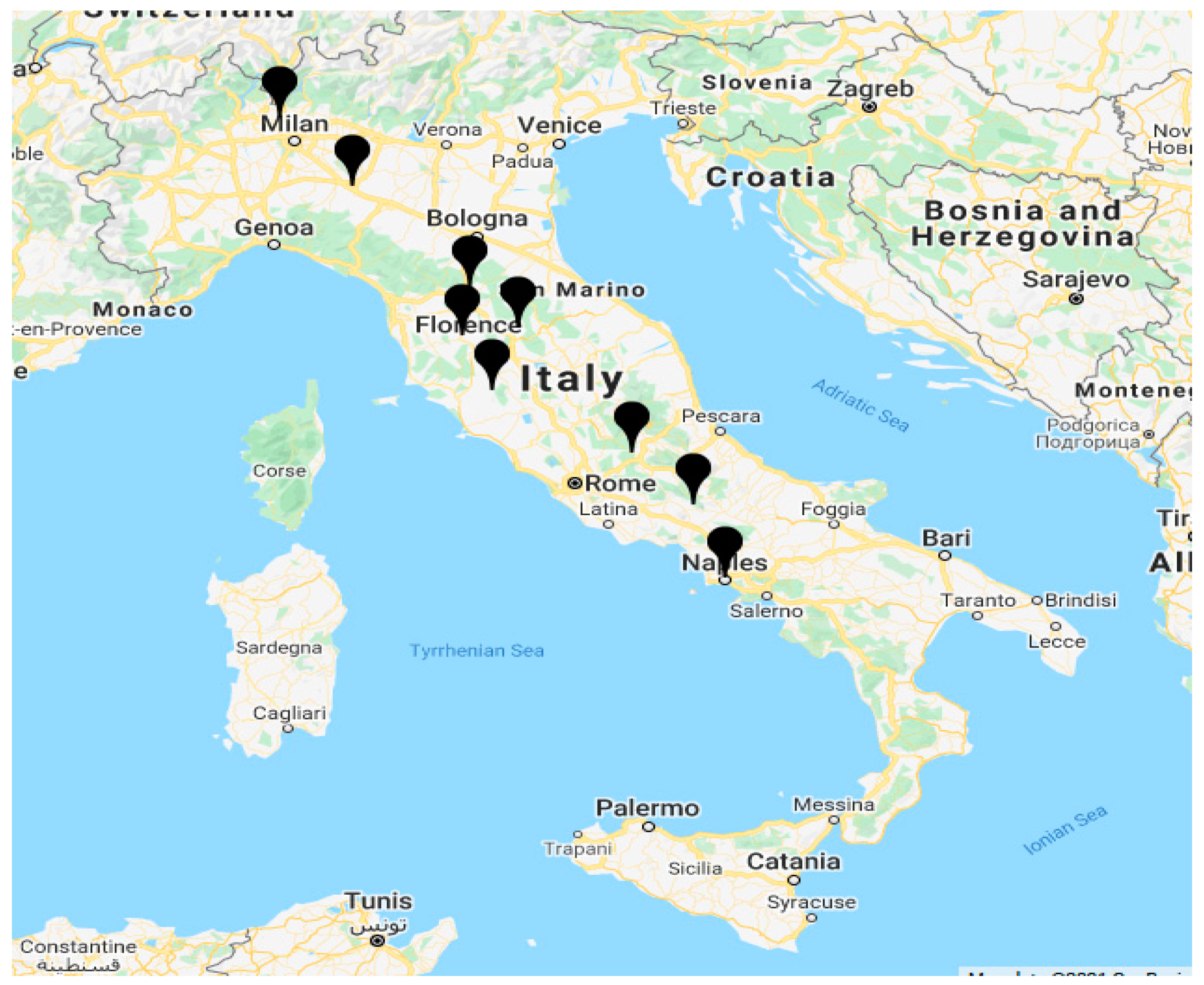
Nine different regions of Italy were taken for study, as mentioned below (Figure 6, projection of waterbodies marked—Aquifer-Auser, Dognella, Luco, Petrignano Lake, Bilancino River, Arno Water Spring, Amiata, Lupa, Madonna di Canneto).

Each water body has unique attributes which are not linked to each other. Each data set consists of 20 years of records (2000–2020). The datasets are entirely independent of each other. Many glasses of water are required for the daily consumption and relevant companies struggle to forecast water availability in a waterbody. Due to climate change, the water level in water bodies has been refilled or started to drain. To help preserve the immunity of these water bodies, there is a necessity to predict the most efficient water availability in terms of level and water flow.

6. Results and Discussion

Datasets of four water bodies were taken for the study, specifically aquifer, lake, river, and water springs. All datasets were divided into three sets: training dataset, validation datasets, and testing datasets with 80/10/10 out of 100. We had both types of variables in data, stationary and non-stationary. We trained VAR (requires stationary variable) and VECM (does not need stationary variable) on the training and validation dataset. In contrast, the LSTM model was only trained on training data and fine-tuned via the validation dataset. All models were tested on a testing dataset of various sizes depending on the amount of non-missing observations available in the different data. For maintaining result accuracy, missing/imputed data were masked. RMSE and MAE were used as evaluation metrics to compare the result.

The table summarizes results for each dataset type collectively using best-suited parameter settings in both VAR/VECM and LSTM. In VAR/VECM, the prediction result was made daily (1 day), the last 7 days, and last 14 days performance results were recorded. The LSTM model predicts for a single day and compares the result before and after scaling the data.

Here, LSTM has not been implemented for 7 days and 14 days of performance in a row. The training/validating/testing sample sizes are negligible due to considerable lag (i.e., lag = 7). This behaves the same as a VAR which does not perform well with a small sample size. The LSTM model used solely focuses on feature importance.

7. Applications of Models to Water Bodies

7.1. Aquifer

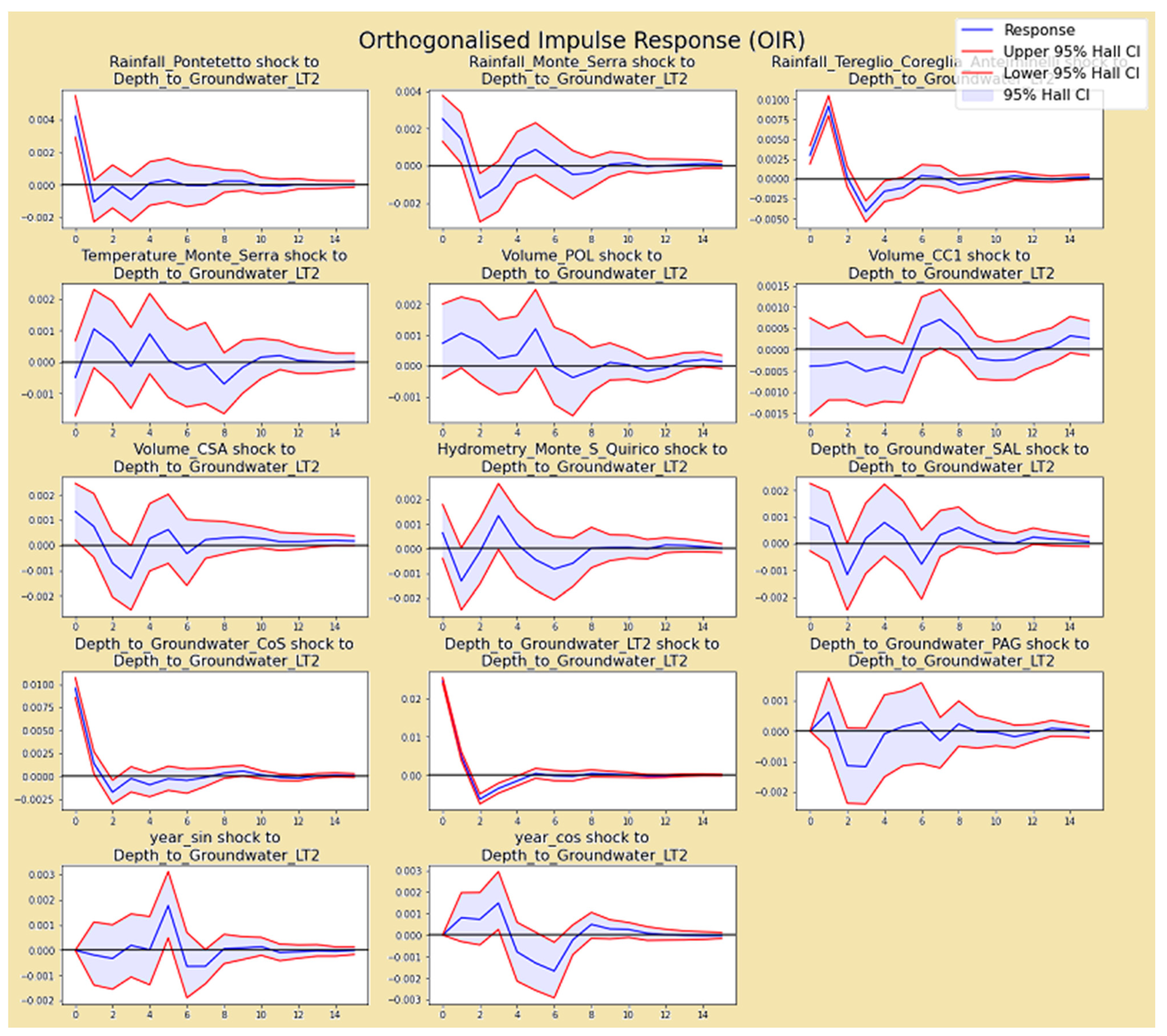
Figure 7 shows the OIR plot for the target variable Depth_to_Groundwater_LT2 of AUSER-AQUIFER. The main idea of the OIR is to notice how one standard deviation shock to x causes a significant (increase/decrease standard deviation) response in y form periods. Symbols mean the response direction.

Generally, the symbol directions make sense (except the Rainfall_Tereglio_Coreglia_Antelminelli for the final feature): A positive shock to rainfall adds water to the aquifer; A positive shock to volume (meaning less water taken from the drinking water plant since the volume is itself negative) leaves more water in the aquifer; a positive shock to hydrometry also means a positive response to groundwater.

Order plays a significant role in the OIR plot. The feature order chosen for aquifer datasets is Rainfall → Temperature → Volumes → Hydrometries → Depth_to_Groundwaters. The order between rainfall and temperature can be reversed since they affect each other. Depth_to_Groundwater is put at the end because we wanted to see how the other features affected the targets. Volumes (the amount taken from the drinking water treatment plant) affect Hydrometries, so Volumes are put before hydrometry. After testing the VAR model on the various setting parameters, the best-suited one was used for comparison with the LSTM model; as shown in Table 1, the Target feature is Depth_to_Groundwater, and the standard features we get after performing the test are hydrometry and rainfall. The Table 1 shows the comparative analysis of VAR and LSTM models.

7.2. Lake

Figure 8 shows the OIR plot for the target variables Flow_Rate and Lake_level of Lake Bilancino. We can conclude from the OIR how one standard deviation shock to Flow_rate/Lake_level causes a significant (increase/decrease standard deviation) response in other variables from the periods.

The feature order chosen for lake datasets is Rainfall → Temperature → Flow_Rate → Lake_Level. The order between rainfall and temperature can be reversed since they affect each other. Lake _level is put at the end because we want to see how the other features affect the targets.

Table 2 summarizes how the VAR model acts better in the long term in comparison to LSTM. The target feature is Flow_Rate and Lake_level, and the common feature after performing the test is Rainfall and Flow_rate. We can say that rainfall has a high impact on the water level in the lake.

7.3. River

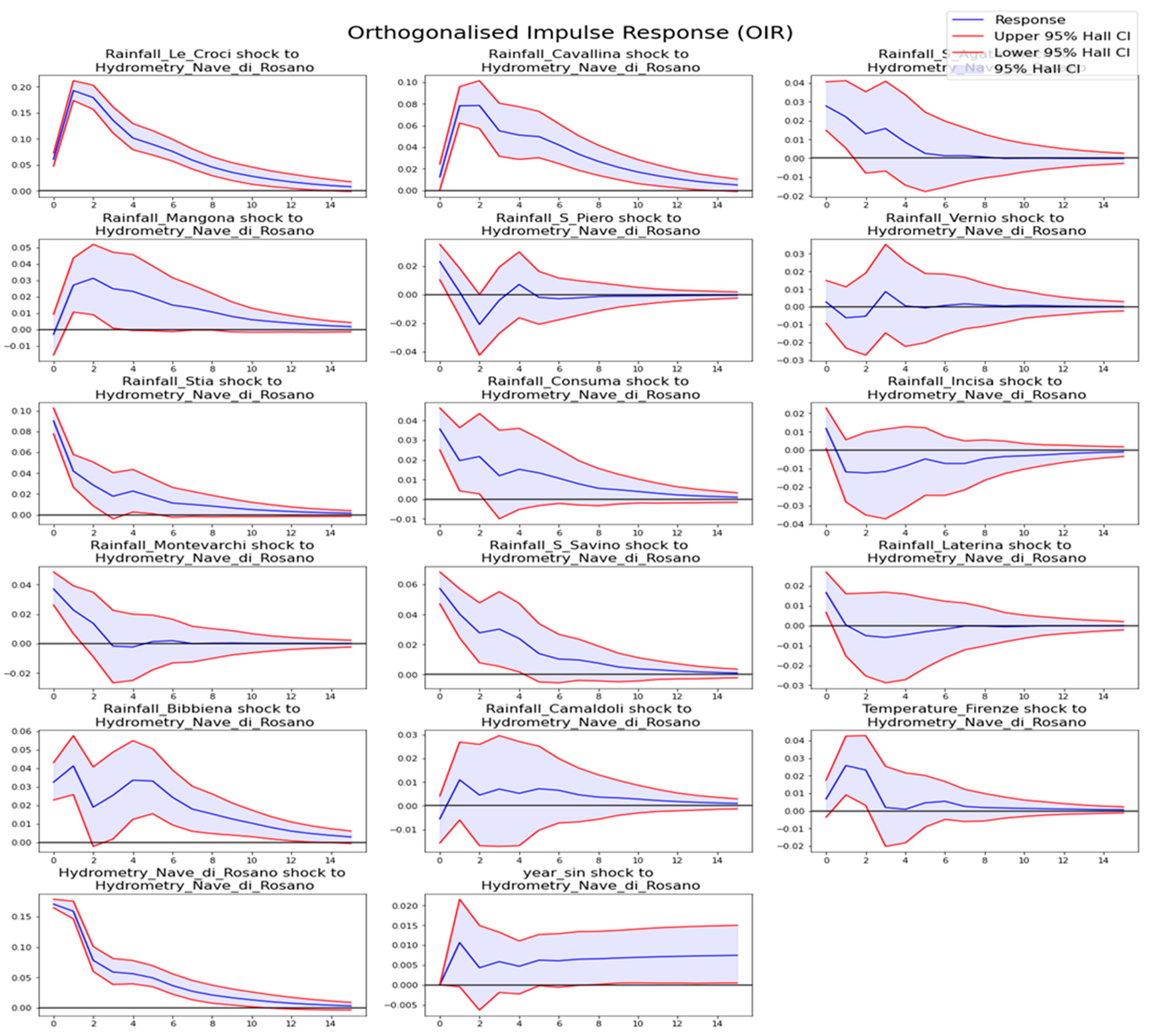
Figure 9 shows the RIVER ARNO OIR plot for the target variable Hydrometry (Flow_rate). The feature order we chose is Rainfall → Temperature → Hydrometry. The former can shock later but not the other way around.

From the sensitivity analysis, we found that Rainfall_Le_Croci, Temperature_Firenze, Rainfall_Cavallina, etc. are essential features to LSTM. However, compared to OIR analysis in VAR, only Rainfall_Cavallina, Rainfall_Le_Croci are in common. We conclude that Rainfall_Cavallina and Le_Croci are the most crucial feature to Hydrometry_Nave_di_Rosano. Other mentioned features are sub-important, part of them for a linear model and a non-linear LSTM model. Table 3 shows a comparative study between VAR and LSTM. The target feature is Hydrometry_Nave_di_Rosano, and the standard features we get after performing the test are Rainfall_Le_Croci, Rainfall_Cavallina.

7.4. Water Springs

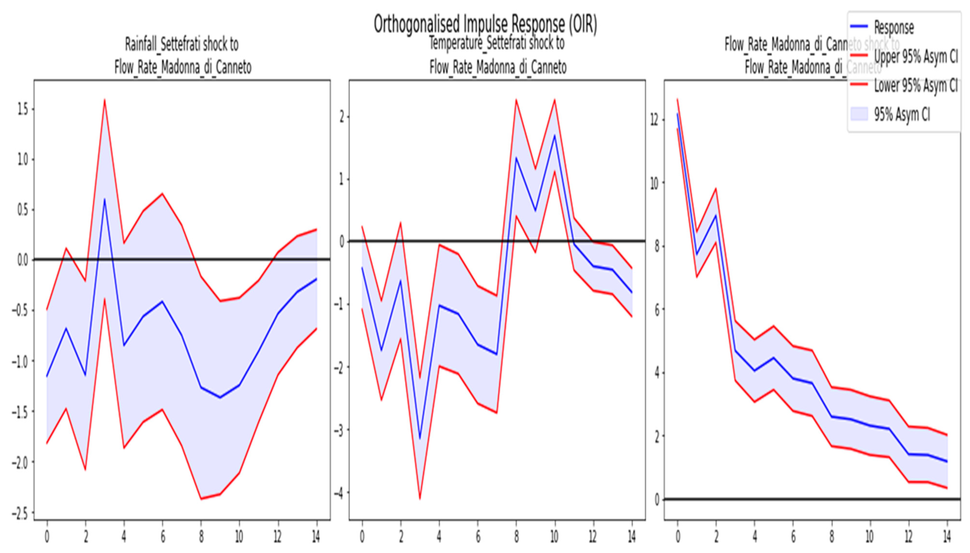
Assuming that the water springs are located on different water bodies, all these water bodies are impacted simultaneously by rainfall and the resulting water flows; however, if the slow decay in the flow rate proportions indicates that the entire rainfall process, the filling of aquifers, and the water flow from the springs takes time and lags. The time series variable shows many lags; this indicates that a long-memory process may lead to better performance. This means that a shock may lead to a relatively persistent change in the water flow. A VECM model could capture this memory. Figure 10 shows the OIR plot for Flow rate shock against rainfall, temperature, and flow rate itself.

From Table 4, we can conclude that for AMIATA VAR. VECM delivers mixed prediction qualities. In the case of LUPA, in comparison to VAR, VECM does not bring any extra benefit. Moving further to MADONNA-DI-CANNETO, VAR seems to be a good choice.

8. Conclusions

When climate change causes irregular rainfall and consumers and regulators demand water, free of chemical pollutants, it is increasingly important to find sustainable water sources. We explored the parametric model, VAR/VECM, to build the best-suited one for each waterbody, inferring causal relationships between different waterbody features. For example—a spring’s flow rate depends partially on the amount of water currently present in its source aquifer. However, the aquifer’s water level also changes due to discharging some water through the spring. The OIR/FEVD plot shows the significance of the chosen features on target features, i.e., how the behavior of one variable concerns other variables in the event of a shock. VECM performs better where a long memory process is required. In water spring, it was noted that a shock may lead to a relatively persistent change in the water flow. Since the VAR model is linear and can only capture local linear prediction, LSTM was implemented to capture the possible non-linear relationship between target and features in the datasets. Due to the missing and unusual pattern in some datasets, we probably have a non-linear pattern, so VAR models may not perform well. We have limited data available to train LSTM, so that the LSTM model results may not be reliable. However, in most cases, we found the VAR model to be more reliable in comparison to LSTM. Although LSTM is not perfectly fine-tuned, it provides decent forecasts. It gives good results on feature importance in most cases. Furthermore, when calculating the MAE/RMSE in each dataset, we scaled the data back to the original levels to reflect the proper performance accurately. In the best situation, a feature was doubly confirmed to be important when the VAR and LSTM models featured analysis to rank it.

In the future, further studies can be carried out to create models that evaluate predictions over longer horizons. Features may interact in different patterns, and early warning signals of shortening water supply may be uncovered. There is also scope of solving water crisis challenges due to climate change by considering climatic conditions that impact water levels/precipitation patterns. In a further study, climatic attributes can be included in the order of events considered to find the casual relationship; this will accelerate the study of the impact of climate on water resources. Additionally, since the data revealed long memory in many cases, a multivariate version of fractional integration (i.e., processes with an order of integration between zero and one) may be helpful to deal with large lag orders. Such models may require fewer parameters and can be used to predict over long horizons. We attempted to tackle the problem of significant lags with the use of VECM models. Due to the use of fewer parameters, the VECM model is recommended for water demand prediction and can aid policy makers and water resource managers in accurate estimation of available water resources at a feasible cost.

References

1. Baer, A. Not enough water to go round? Int. Soc. Sci. J. 1996, 48, 277–292. [Google Scholar] [CrossRef]
2. Yuan, X.; Wu, X.; Tian, H.; Yuan, Y.; Adnan, R.M. Parameter Identification of Nonlinear Muskingum Model with Backtracking Search Algorithm. Water Resour. Manag. 2016, 30, 2767–2783. [Google Scholar] [CrossRef]
3. Salem, G.S.A.; Kazama, S.; Shahid, S.; Dey, N.C. Impact of temperature changes on groundwater levels and irrigation costs in a groundwater-dependent agricultural region in northwest Bangladesh. Hydrol. Res. Lett. 2017, 11, 85–91. [Google Scholar] [CrossRef] [Green Version]
4. Bayatvarkeshi, M.; Zhang, B.; Fasihi, R.; Adnan, R.M.; Kisi, O.; Yuan, X. Investigation into the Effects of Climate Change on Reference Evapotranspiration Using the HadCM3 and LARS-WG. Water 2020, 12, 666. [Google Scholar] [CrossRef] [Green Version]
5. U.S. Geological Survey. Available online: https://www.usgs.gov/special-topic/water-science-school/science/a-comprehensive-study-natural-water-cycle?qt-science_center_objects=0#qt-science_center_objects (accessed on 18 January 2021).
6. Alizamir, M.; Kisi, O.; Adnan, R.M.; Kuriqi, A. Modelling reference evapotranspiration by combining neuro-fuzzy and evolutionary strategies. Acta Geophys. 2020, 68, 1113–1126. [Google Scholar] [CrossRef]
7. Yuan, X.; Chen, C.; Lei, X.; Yuan, Y.; Adnan, R.M. Monthly runoff forecasting based on LSTM–ALO model. Stoch. Environ. Res. Risk Assess. 2018, 32, 2199–2212. [Google Scholar] [CrossRef]
8. Donkor, E.A.; Mazzuchi, T.A.; Soyer, R.; Roberson, J.A. Urban Water Demand Forecasting: Review of Methods and Models. J. Water Resour. Plan. Manag. 2014, 140, 146–159. [Google Scholar] [CrossRef]
9. Chen, J.; Boccelli, D.L. Forecasting Hourly Water Demands with Seasonal Autoregressive Models for Real-Time Application. Water Resour. Res. 2018, 54, 879–894. [Google Scholar] [CrossRef]
10. Muhammad Adnan, R.; Yuan, X.; Kisi, O.; Yuan, Y.; Tayyab, M.; Lei, X. Application of soft computing models in streamflow forecasting. In Proceedings of the Institution of Civil Engineers-Water Management; Thomas Telford Ltd.: London, UK, 2019; Volume 172, No. 3. pp. 123–134. [Google Scholar]
11. Gujarati, D.N. Basic Econometrics; Tata McGraw-Hill Education: New York, NY, USA, 2009. [Google Scholar]
12. Adnan, R.M.; Liang, Z.; Yuan, X.; Kisi, O.; Akhlaq, M.; Li, B. Comparison of LSSVR, M5RT, NF-GP, and NF-SC Models for Predictions of Hourly Wind Speed and Wind Power Based on Cross-Validation. Energies 2019, 12, 329. [Google Scholar] [CrossRef] [Green Version]
13. Kisi, O.; Shiri, J.; Karimi, S.; Adnan, R.M. Three different adaptive neuro fuzzy computing techniques for forecasting long-period daily streamflows. In Big Data in Engineering Applications; Springer: Singapore, 2018; pp. 303–321. [Google Scholar]
14. Lütkepohl, H. Vector autoregressive models. In Handbook of Research Methods and Applications in Empirical Macroeconomics; Edward Elgar Publishing: Camberley, UK, 2013. [Google Scholar] [CrossRef] [Green Version]
15. Mehmood, A.; Jia, S.; Lv, A.; Zhu, W.; Mahmood, R.; Saifullah, M.; Adnan, R.M. Detection of Spatial Shift in Flood Regime of the Kabul River Basin in Pakistan, Causes, Challenges, and Opportunities. Water 2021, 13, 1276. [Google Scholar] [CrossRef]
16. Mitchell, T.M. The Discipline of Machine Learning; Carnegie Mellon University, School of Computer Science, Machine Learning Department: Pittsburgh, PA, USA, 2006; Volume 9. [Google Scholar]
17. Provost, F. Machine learning from imbalanced data sets 101. In Proceedings of the AAAI’2000 Workshop on Imbalanced Data Sets; AAAI Press: Palo Alto, CA, USA, 2000; pp. 1–3. [Google Scholar]
18. Vellido, A.; Martin-Guerrero, J.D.; Lisboa, P.J.G. Making machine learning models interpretable. In Proceedings of the ESANN, European Symposium on Artificial Neural Networks, Computational Intelligence and Machine Learning, Bruges, Belgium, 25–27 April 2012; Volume 12, pp. 163–172. [Google Scholar]
19. Groenen, I. Master Thesis: Representing Seasonal Patterns in Gated Recurrent Neural Networks for Multivariate Time Series Forecasting. 2018. Not Yet Online; Confidential. Available online: http://www.scriptiesonline.uba.uva.nl/657906 (accessed on 20 October 2018).
20. Bontsema. Master Thesis: Forecasting Ammonium Concentration in Wastewater Treatment Plant. 2018. Available online: https://beta.vu.nl/nl/onderwijs/project-en-stage/stagebureau-wiskunde-informatica/master-project-ba/stageverslagen-online/index.aspx (accessed on 25 January 2021).
21. Adnan, R.M.; Liang, Z.; El-Shafie, A.; Zounemat-Kermani, M.; Kisi, O. Prediction of Suspended Sediment Load Using Data-Driven Models. Water 2019, 11, 2060. [Google Scholar] [CrossRef] [Green Version]
22. LeCun, Y.; Bengio, Y.; Hinton, G. Deep learning. Nature 2015, 521, 436–444. [Google Scholar] [CrossRef] [PubMed]
23. Xiang, Z.; Yan, J.; Demir, I. A Rainfall-Runoff Model with LSTM-Based Sequence-to-Sequence Learning. Water Resour. Res. 2020, 56, 1. [Google Scholar] [CrossRef]
24. Elsheikh, A.H.; Katekar, V.P.; Muskens, O.L.; Deshmukh, S.S.; Elaziz, M.A.; Dabour, S.M. Utilization of LSTM neural network for water production forecasting of a stepped solar still with a corrugated absorber plate. Process. Saf. Environ. Prot. 2021, 148, 273–282. [Google Scholar] [CrossRef]
25. Barzegar, R.; Aalami, M.T.; Adamowski, J. Short-term water quality variable prediction using a hybrid CNN–LSTM deep learning model A Short-Term Data Based Water Consumption Prediction Approach. Stoch. Environ. Res. Risk Assess. 2020, 34, 1–19. [Google Scholar] [CrossRef]
26. Xu, Z.; Ying, Z.; Li, Y.; He, B.; Chen, Y. Pressure prediction and abnormal working conditions detection of water supply network based on LSTM. Water Supply 2020, 20, 963–974. [Google Scholar] [CrossRef]
27. McCracken, M.W.; McGillicuddy, J.T. An empirical investigation of direct and iterated multistep conditional forecasts. J. Appl. Econ. 2019, 34, 181–204. [Google Scholar] [CrossRef]
28. Zhao, J.; Mu, X.; Gao, P. Dynamic response of runoff to soil and water conservation measures and precipitation based on VAR model. Hydrol. Res. 2019, 50, 837–848. [Google Scholar] [CrossRef]
29. Keng, C.Y.; Shan, F.P.; Shimizu, K.; Imoto, T.; Lateh, H.; Peng, K.S. AIP Conference Proceedings Application of vector autoregressive model for rainfall and groundwater level analysis. In Proceedings of the 24th National Symposium on Mathematical Sciences: Mathematical Sciences Exploration for the Universal Preservation, Kuala Terengganu, Malaysia, 27–29 September 2016. [Google Scholar] [CrossRef]
30. Hartini, S.; Hadi, M.P.; Sudibyakto, S.; Poniman, A. Application of Vector Auto Regression Model for Rainfall-River Discharge Analysis. Forum Geogr. 2015, 29, 1–10. [Google Scholar] [CrossRef] [Green Version]
31. Pradhan, R.P.; Bagchi, T.P. Effect of transportation infrastructure on economic growth in India: The VECM approach. Res. Transp. Econ. 2013, 38, 139–148. [Google Scholar] [CrossRef]
32. Honkatukia, J.; Malkonen, V.; Perrels, A. Impacts of the European Emissions Trade System on Finnish Wholesale Electricity Prices; Government Institute for Economic Researchs: Helsinki, Finland, 2006. [Google Scholar]
33. Fell, H. EU-ETS and Nordic Electricity: A CVAR Analysis. Energy J. 2010, 31, 1–25. [Google Scholar] [CrossRef] [Green Version]
34. Chemarin, S.; Heinen, A.; Strobl, E. Electricity, Carbon and Weather in France: Where do We Stand? Ecole Polytechnique, Centre National de la Recherche Scientifique: Paris, France, 2008. [Google Scholar]
35. Thoenes, S. Understanding the Determinants of Electricity Prices and the Impact of the German Nuclear Moratorium; Institute of Energy Economics at the University of Cologne (EWI): Cologne, Germeny, 2011. [Google Scholar]
36. Loves, L.; Usman, M.; Russel, E. Modeling Multivariate Time Series by Vector Error Correction Models (VECM) (Study: PT Kalbe Farma Tbk. and PT Kimia Farma (Persero) Tbk). In Journal of Physics: Conference Series; IOP Publishing: Bristol, UK, 2021. [Google Scholar] [CrossRef]
37. Enders, W. Applied Econometric Time Series; John Wiley and Sons Interscience Publication: Hoboken, NJ, USA, 2015. [Google Scholar]
38. Asteriou, D.; Hall, S.G. Applied Econometrics: A Modern Approach; Palgrave Macmillan: New York, NY, USA, 2007. [Google Scholar]
39. Lutkepohl, H. New Introduction to Multiple Time Series Analysis; Springer: Heidelberg, Germany, 2005. [Google Scholar]
40. Duan, Y.; Lv, Y.; Wang, F. Travel time prediction with LSTM neural network. In Proceedings of the IEEE 19th International Conference on Intelligent Transportation Systems (ITSC), Rio de Janeiro, Brazil, 1–4 November 2016; pp. 1053–1058. [Google Scholar] [CrossRef]
41. MAE and RMSE—Which Metric Is Better?-Human in Machine World, Medium. 2016. Available online: https://medium.com/human-in-a-machine-world/mae-and-rmse-which-metric-is-better-e60ac3bde13d (accessed on 25 February 2021).
42. Tayyab, M.; Zhou, J.; Zeng, X.; Zhao, N.; Adnan, R. Integrated Combination of the Multi Hydrological Models by Applying the Least Square Method. Res. J. Appl. Sci. Eng. Technol. 2015, 10, 107–111. [Google Scholar] [CrossRef]
43. Tayyab, M.; Zhou, J.; Adnan, R.; Meng, C.; Zahra, A. Streamflow Prediction by Applying Generalized Regression Network with Time Series Decomposition Method. Indones. J. Electr. Eng. Comput. Sci. 2016, 4, 611–616. [Google Scholar] [CrossRef]
44. Yuan, X.; Tian, H.; Yuan, Y.; Huang, Y.; Ikram, R.M.A. An extended NSGA-III for solution multi-objective hydro-thermal-wind scheduling considering wind power cost. Energy Convers. Manag. 2015, 96, 568–578. [Google Scholar] [CrossRef]
45. Adnan, M.; Nabi, G.; Kang, S.; Zhang, G.; Adnan, R.M.; Anjum, M.N.; Iqbal, M.; Ali, A.F. Snowmelt Runoff Modelling under Projected Climate Change Patterns in the Gilgit River Basin of Northern Pakistan. Pol. J. Environ. Stud. 2017, 26, 525–542. [Google Scholar] [CrossRef]
46. Adnan, R.M.; Parmar, K.S.; Heddam, S.; Shahid, S.; Kisi, O. Suspended Sediment Modeling Using a Heuristic Regression Method Hybridized with Kmeans Clustering. Sustainability 2021, 13, 4648. [Google Scholar] [CrossRef]
Figure 1. The structure of the LSTM cell.
Climate 09 00144 g001
Figure 2. Flowchart of working model VAR/VECM.
Climate 09 00144 g002
Figure 3. Variable distribution of the Petrignano-aquifer.
Climate 09 00144 g003
Figure 4. An example of the Granger Causality test (Bilancino-Lake).
Climate 09 00144 g004
Figure 5. LSTM feature importance for Auser-Aquifer.
Climate 09 00144 g005
Figure 6. Map showing all nine different regions under study.
Climate 09 00144 g006
Figure 7. OIR plot for Depth_to_Groundwater_LT2 (AUSER-AQUIFER).
Climate 09 00144 g007
Figure 8. OIR plot for Flow_rate and Lake_level (LAKE-BILANCINO).
Climate 09 00144 g008
Figure 9. OIR plot of Hydrometry_Nave_di_Rosano(Flow_rate)-RIVER-ARNO.
Climate 09 00144 g009
Figure 10. OIR plot for Flow_Rate (Water Springs-Madonna_di_Canneto).
Climate 09 00144 g010