Solar and Anthropogenic Influences on Climate: Regression Analysis and Tentative Predictions

Abstract

The paper aims to quantify solar and anthropogenic influences on climate change, and to make some tentative predictions for the next hundred years. By means of double regression, we evaluate linear combinations of the logarithm of the carbon dioxide concentration and the geomagnetic aa index as a proxy for solar activity. Thereby, we reproduce the sea surface temperature (HadSST) since the middle of the 19th century with an adjusted $R^2$ value of around 87 percent for a climate sensitivity (of TCR type) in the range of 0.6 K until 1.6 K per doubling of CO${}_2$. The solution of the double regression is quite sensitive: when including data from the last decade, the simultaneous occurrence of a strong El Niño and of low aa values leads to a preponderance of solutions with relatively high climate sensitivities around 1.6 K. If these later data are excluded, the regression delivers a significantly higher weight of the aa index and, correspondingly, a lower climate sensitivity going down to 0.6 K. The plausibility of such low values is discussed in view of recent experimental and satellite-borne measurements. We argue that a further decade of data collection will be needed to allow for a reliable distinction between low and high sensitivity values. In the second part, which builds on recent ideas about a quasi-deterministic planetary synchronization of the solar dynamo, we make a first attempt to predict the aa index and the resulting temperature anomaly for various typical CO${}_2$ scenarios. Even for the highest climate sensitivities, and an unabated linear CO${}_2$ increase, we predict only a mild additional temperature rise of around 1 K until the end of the century, while for the lower values an imminent temperature drop in the near future, followed by a rather flat temperature curve, is prognosticated.

1. Introduction

As the heir of great pioneers [1,2], modern climate science [3] has had major difficulties in narrowing down its most prominent parameter—equilibrium climate sensitivity (ECS)—from the ample range 1.5–4.5 K (per $2\times$ CO${}_2$) that was already given in the Charney report [4]. This lack of specificity is sometimes discussed in terms of various interfering socio-scientific and political factors [5,6]. Yet, in addition to those more “subjective” reasons for climate predictions to be that vague, there are at least two “objective” ones: the paucity of precise and reliable experimental measurements of the climate sensitivity, and the unsatisfying state of understanding the complementary solar influence on the climate. Notably, a couple of mechanisms have been proposed [7,8,9] that could significantly surmount the meager 0.1 percent variation of the total solar irradiance (TSI) which is routinely used as an argument against any discernible solar impact on the climate. Among those mechanisms, the following ones figure most prominently: the comparable large variation of the UV component with its influence on the ozone layer and the resulting stratospheric–tropospheric coupling [10,11,12,13,14,15]; the effects of solar magnetic field-modulated cosmic rays on aerosols and clouds [16,17,18,19]; downward winds following geomagnetic storms in the polar caps of the thermosphere, penetrating the stratosphere and troposphere [20]; the solar wind’s impact on the global electric current [21,22]; the (UV) radiation effects on the growth of oceanic phytoplankton [23], which, in turn, produces dimethylsulphide, a major source of cloud condensation nuclei [24]. However, even the very TSI is suspected [7,25,26,27] to have risen much more steeply since the Little Ice Age than assumed in conservative estimations [28,29,30]. While neither of those mechanisms can presently be considered as conclusively proven [8,31,32], they all together entail significantly more potential for solar influence on the terrestrial climate than what is usually discussed [33]. Any resonance-like interaction of solar forcing with the intrinsic dynamics of the climate system (cf. [34] concerning the “stadium wave”, or [35,36] concerning sub-harmonic Rossby waves) would add further interesting aspects to this issue.

In view of claims [37] of an overwhelming scientific consensus on this complex and vividly debated research topic, and the severe political consequences drawn from it, we reiterate here Parker’s prophetic warning [38] that “…it is essential to check to what extend the facts support these conclusions before embarking on drastic, perilous and perhaps misguided plans for global action”. We also agree with his “…inescapable conclusion (…) that we will have to know a lot more about the sun and the terrestrial atmosphere before we can understand the nature of contemporary changes in climate”.

Thus motivated, and also provoked by recent experimental [39] and satellite-borne measurements [40,41] pointing consistently to a rather low climate sensitivity, we perform another attempt to quantify the respective shares of solar and anthropogenic climate drivers. Specifically, we resume the long tradition of correlating terrestrial temperature data with certain proxies of solar activity, as pioneered by Reid [42] for the sunspot numbers, by Friis-Christensen and Lassen [43] and Solheim et al. [44] for the solar cycle length, and by Cliver et al. [45] and Mufti and Shah [46] for the geomagnetic aa index [47]. Our work builds strongly on the two latter papers, which—based on data ending in 1990 and 2007, respectively—had found empirical correlation coefficients between the aa index and temperature variations of up to 0.95. Notwithstanding some doubts regarding their statistical validity [48], such remarkably high correlations might rise the provocative question of whether any sort of greenhouse effect is still needed at all to explain the (undisputed) global warming over the last one and a half centuries. More recently, however, any prospects for such a reversed simplification were dimmed by the fact that the latest decline of the aa index was not accompanied by a corresponding drop of temperature. By contrast, the latter remained rather constant during the first one and a half decades of the 21st century (the “hiatus”), and even increased with the recent strong El Niño events.

This paper aims at supplementing those previous works [45,46,49,50] by taking seriously into account both observations: the nearly perfect correlation of solar activity with temperatures over about 150 years, and the notable divergence between these quantities during the last two decades. In Section 2, using a double regression analysis, quite similar to that of Soon et al. [51], but with the time series of the aa index as the second independent variable (in addition to the logarithm of CO${}_2$ concentration), we show that the temperature variation since the middle of the 19th century can be reproduced with an (adjusted) $R^2$ value of about 87 percent. Such a goodness-of-fit is achieved for specific combinations of the weights of the aa index and of CO${}_2$ that form a nearly linear function in their two-dimensional parameter space. Best results are obtained for a climate sensitivity in the range between 0.6 and 1.6 K (per 2× CO${}_2$), with a delicate dependence on whether the latest data are included or not. Derived from empirical variations on the (multi-)decadal time scale, this climate sensitivity should be interpreted as a sort of transient climate response (TCR), rather than an ECS. Our range corresponds well with that of Lewis and Curry [52], 0.8–1.3 K, but is somewhat lower than the “official” 1.0–2.5 K range [3]. The lower edge of our estimation is plausibilized by recent experimental [39] and satellite-borne measurements [40,41]. It is also quite close, although still higher, than the particularly low estimate of less than 0.44 K, as advocated by Soon et al. [53] after comparing exclusively rural temperature data in the Northern hemisphere with the TSI. The upper edge, in turn, is not far from the spectroscopy-based estimation by van Wijngaarden and Happer [54]. We also argue that at least one additional decade of data collection will be needed to finally decide between low and high sensitivity values.

With the complementary share of the Sun for global warming reaching values between 30 and 70 percent, any climate forecast requires a decent forecast of solar activity. This leads us into yet another controversial playing field, viz, the predictability of the solar dynamo. While the existence of the short-term Schwabe/Hale cycle is a truism in solar physics, the existence and/or stability of the mid-term Gleissberg and Suess-de Vries cycles are already controversially discussed, and there is even more uncertainty about long-term variations such as the Eddy and Hallstatt “cycles”, which are closely related to the sequence of Bond events [55].

In a series of recent papers [56,57,58,59,60,61,62], we have tried to develop a self-consistent explanation of these short-, medium- and long-term solar cycles in terms of synchronization by planetary motions. According to our present understanding, the surprisingly phase-stable 22.14-year Hale cycle [23,61] results from parametric resonance of a conventional $\alpha -\Omega$ dynamo with an oscillatory part of the helical turbulence parameter $\alpha$ that is thought to be synchronized by the 11.07-year spring-tide periodicity of the three tidally dominant planets Venus, Earth and Jupiter [56,57,58,59]. The medium-term Suess-de Vries cycle (specified to 193 years in our model) then emerges as a beat period between the basic 22.14-year Hale cycle and some (yet not well understood) spin–orbit coupling connected with the motion of the Sun around the barycenter of the solar system that is governed by the 19.86-year synodic period of Jupiter and Saturn [60,62]. Closely related to this, Gleissberg-type cycles appear as nonlinear beat effects and/or from perturbations of the Sun’s orbital motion due to other synodic periods of the Jovian planets. Finally, the long-term variations on the millennial time-scale (Bond events) arise as chaotic transitions between regular and irregular episodes of the solar dynamo [62], in close analogy with the super-modulation concept introduced by Weiss and Tobias [63].

Being well aware of the conjectural nature of this synchronized solar dynamo model, in Section 3 we make a tentative prediction of the aa index for the next 130 years, based on simple three-frequency fits to the aa index data over the last 170 years. While our choice for three frequencies is motivated by the dominance of one Suess-de Vries and two Gleissberg-type cycles, we employ different versions of fixing or relaxing their frequencies, which leads to a certain variety of forecasts. A common feature of all of them is, however, a noticeable decline of solar activity until 2100, and a recovery in the 22nd century. These predictions for the aa index are then combined with three different scenarios of CO${}_2$ increase, including an unfettered annual increase by 2.5 ppm and two further scenarios based on hypothetical decarbonization schemes. The $3\times 3$ models thus obtained are then blended with the different combinations of weights for the aa index and CO${}_2$ as derived before in the regression analysis. For the “hottest” scenario, we predict an additional temperature increase until 2100 of approximately 1 K, while all other combinations lead to less warming, partly even to some imminent cooling, followed by a rather flat behaviour in which decreasing solar activity and a mildly increasing trend from CO${}_2$ compensate each other to a large extent. In Section 4 our results are summarized, and some conclusions are drawn in Section 5.

2. Double Regression Analysis

In this section, we perform a double regression analysis of the temperature data (dependent variable) on the geomagnetic aa index and the logarithm of CO${}_2$ (independent variables). We conduct this in an intuitive and easily reproducible way by showing the fraction of variance unexplained ($\mathrm{FVU}$), i.e., the ratio of the residual sum of squares to the total sum of squares, whose minimum was then identified. From these $\mathrm{FVU}$s, we derive the corresponding $R^2$ value, both in its usual and in its adjusted variant. Let us start, however, with a description of our data base.

2.1. Data

While reliable CO${}_2$ data are obtainable for a long period of time, we decided to restrict our data base to the time from the middle of the 19th century, for which both temperature data and the aa index are readily available.

2.1.1. Temperature Data

There are quite a number of different temperature series which might be considered as the basis for a regression analysis. In order to make contact with the work of Mufti and Shah [46], we decided to use the Hadley Centre Sea Surface Temperature (HadSST) dataset in its updated version HadSST.4.0.0.0, available from www.metoffice.gov.uk (accessed on 1 August 2021) which provided us with the sea surface temperature anomaly from 1850 to 2018, relative to the 1961–1990 average [64]. Actually, these data are not gravely different from the combined sea/land surface temperature (HadCRUT), apart from some slight, but systematic, divergence during the last two decades (the tendency for enhanced warming over land has been discussed in terms of the surface energy balance by Sutton et al. [65], although non-climatic biases in land surface temperature records, such as the urban heat island (UHI) effect [66], might also play a role here).

The HadSST data are shown as open circles in Figure 1a, together with two exemplary centered moving averages with windows 11 years (full line) and 23 years (dashed line), which we will frequently refer to in the following. These curves show the typical temporal structure comprising a slow decay between 1850 and 1905, a rather steep rise between 1905 until 1940, again a mild decay until 1970, followed by a steep increase until 1998. As for the last two decades, we first observe the “hiatus” between 1999 and 2014, being then overwhelmed by the recent strong El Niño events. We will return to those latest years further below.

2.1.2. Geomagnetic aa Index Data

A widely used measure of solar activity, the aa index represents the amplitude (in nT) of the global geomagnetic activity during 3 h intervals at two antipodal magnetic observatories, normalized to geomagnetic latitude $\pm {50}^{°}$ [47]. Inspired by the work of Cliver et al. [45] and Mufti and Shah [46], who pointed out the remarkable correlation of up to 0.95 between (time averaged) temperature anomalies and the geomagnetic aa index, we use the latter data as a proxy for solar activity (slight corrections of this attribution might result from taking into account the weakly confounding factors related to the secular change of the orientation and strength of the Earth’s magnetic field, as discussed previously [67]). A viable alternative would have been to use sunspot data, or various versions of the TSI, as exemplified in [27,53]. Given, on one side, their generally high correlation ($r=0.96$) with sunspot numbers [68], and, on the other side, their high reliability based on precise measurement down to 1844 (which avoids some ambiguities concerning the correct variability of the TSI [27,53]), we focus here exclusively on the aa index data, leaving regression analyses with other solar data to future work.

The bulk of the aa index data, between 1868 and 2010, was obtained from the ftp server ftp.ngdc.noaa.gov. As in Reference [46], the early segment between 1844 and 1867 was taken from Nevanlinna and Kataja [69]. The latest segment, between 2011 and 2018, was obtained from www.geomag.bgs.ac.uk (accessed on 1 August 2021). All these aa index data were annually averaged to provide a homogeneous dataset. Together with their 11-year and 23-year moving averages, the annual $\mathrm{aa}$ data are shown in Figure 1b. Already by visual inspection, between 1850 and 1990, we observe a remarkable similarity of their shape with that of temperature, while after 1995, the aa index declined, whereas the temperature continued to increase. We will have more to say on that divergence further below.

2.1.3. CO${}_2$ Data

The CO${}_2$ concentration data until 2014 were obtained from iac.ethz.ch/CMIP6/. The four additional data points from 2015 and 2018 were taken from the website www.co2.earth (accessed on 27 November 2020). Together with their 11-year and 23-year moving averages, the logarithm of these data is shown in Figure 1c. The use of the logarithm relies on the saturation effect according to which it becomes increasingly difficult for additionally added CO${}_2$ molecules to further close the “infrared window” for outgoing radiation.

2.2. The Most Relevant Data and Their Correlations

After presenting the data that will actually be used in the remainder of this paper, we redtake a short break to consider whether these are indeed the most relevant data. Our reliance on the aa index might indeed be questioned, as other studies [6] have claimed a strong temperature dependence on ocean–atmosphere variations, such as the Pacific Decadal Oscillation (PDO) [70] and the Atlantic Multidecadal Oscillation (AMO) [71], with their similar time structures governed by a sort of 60–70-year “cyclicity”. On the other hand, there is also evidence for direct correlations of the aa index with regional features, such as the Northern Annular Mode (NAM) [72]. In order to assess such possible links, in Figure 2 we show exemplarily the 23-year averages of the AMO and the PDO data, together with the previously shown aa index (appropriately shifted and scaled) and $\Delta T$. It is clearly seen that the aa index and $\Delta T$ had a particularly parallel behaviour until 1990. There is also some similarity with AMO, while PDO has a different time dependence.

In

Table 1. Empirical correlation coefficients r between different datasets, each of which represents a centered moving average over 11 or 23 years. The values in parentheses indicate the (one-sided) p-values, based on the “honest” number of degrees of freedom, i.e., $N_{\mathrm{y}}/11$ or $N_{\mathrm{y}}/23$, wherein $N_{\mathrm{y}}$ is the number of years. Note the large values for the correlation both between CO${}_2$ and the aa index with $\Delta T$, compared to weak or barely existing correlations of the AMO and PDO index with $\Delta T$.

	MAW 11 Years: 1855 till			MAW 23 Years: 1867 till
Correlated Data	2013	2008	2003	2008	2003	1998
CO${}_2$ with aa	0.440	0.606	0.720	0.703	0.783	0.803
(one-sided p)	(0.053)	(0.0099)	(0.0017)	(0.045)	(0.023)	(0.02)
CO${}_2$ with $\Delta T$	0.926	0.911	0.891	0.916	0.894	0.869
(one-sided p)	(0)	(0)	(0)	(0.0017)	(0.0037)	(0.0073)
aa with $\Delta T$	0.595	0.738	0.819	0.806	0.900	0.950
(one-sided p)	(0.010)	(0.001)	(0.0001)	(0.016)	(0.0032)	(0.0005)
AMO with $\Delta T$				0.260	0.164	0.106
(one-sided p)				(0.30)	(0.38)	(0.42)
aa with AMO				−0.015	−0.013	−0.028
(one-sided p)				(0.49)	(0.40)	(0.48)
PDO with $\Delta T$				−0.131	−0.001	0.126
(one-sided p)				(0.40)	(0.50)	(0.41)
aa with PDO				0.050	0.049	0.074
(one-sided p)				(0.46)	(0.46)	(0.44)

, we quantify those relationships between various data in terms of the empirical correlation coefficients r (including also the associated one-sided p-values). We perform this for the two different moving average windows (abbreviated henceforth as “MAW”) of 11 years and 23 years, and in either case for three different end points of the time interval (2013, 2008, 2003 for $\mathrm{MAW}=11$ years and 2008, 2003 and 1998 for $\mathrm{MAW}=23$ years; note that these are the centered points of the last interval of the moving averages, into which the annual data from later years are included). Our first observation (see the first row) is the significant correlation between the two predictor variables CO${}_2$ and the aa index. Although we consider both variables as physically independent from each other (while the independence of $\mathrm{aa}$ from CO${}_2$ is evident, we also presume here the CO${}_2$ increase as being exclusively of anthropogenic origin—a certain amount of ”degassing” of the oceans due to heliogenic warming is not completely excluded, but very likely a minor effect), this multicollinearity is at the root of the ill-posedness of our attribution problem. Indeed, both correlations of CO${}_2$ and the aa index with $\Delta T$ have similar r-values in the range between 0.6 and 0.95, which is a first indication for their comparable influences. However, there are some subtleties to discern when considering different end years, both for $\mathrm{MAW}=11$ years and for $\mathrm{MAW}=23$ years. Focusing on the latter case, the correlation for CO${}_2$ acquires its highest value ($r=0.916$) for the full time interval, and decreases slightly to 0.869 when the time interval is shortened by 10 years. By contrast, the correlation of the aa index with $\Delta T$ has only a value of $r=0.8$ for the full interval, but grows to 0.95 for the restricted interval. This latter result confirmed that of Mufti and Shah [46] obtained for a similar period, and by Cliver et al. [45] for a still shorter interval. Some further correlations are indicated exclusively for $\mathrm{MAW}=23$ years. Given the visual similarity of AMO and $\Delta T$ in Figure 2, their correlation is surprisingly small, but would increase if the overall upward trend of $\Delta T$ were subtracted. The PDO seems to show no relevant correlation with $\Delta T$.

In Figure 3, we show some further correlation dependencies, this time on the time shift $\delta t$ between the two respective data, which could possibly give a clue about intrinsic delay effects (such as the ”stadium wave” of [71]). One curve shows the correlation between the aa index and the AMO index, whereby the aa index at earlier times is correlated with AMO at later times. While the correlation is not large, we see at least a clear maximum at $\delta t=11$ years, as if the AMO index lagged behind the aa index by this delay time. The second curve shows the corresponding relationship between $\Delta T$ and AMO, with the correlation reaching a maximum of 0.3 at $\delta t=6$ years. While this looks like a sort of inverted causality (AMO lags behind $\Delta T$), it could simply mean that $\Delta T$ is indeed governed by the aa index, which also determines the AMO index at later times.

We also show the corresponding curves for the aa index and $\Delta T$, in the two versions for the full time interval and the 10-year shortened one. For the full interval, r starts at value 0.8 for $\delta t=0$, but reaches a maximum of 0.915 for $\delta t=10$ years. While at face value this insinuates a 10-years lag between the aa index and $\Delta T$, it is more likely connected with the implied cancellation of the last 10 years during which the aa index was decreasing. In order to test this, in the second curve we omit the last 10 years of both data completely. Here, we find an $r=0.95$ at $\delta t=0$, which still increases to a maximum of $r=0.962$ at $\delta t=3$ yr. This sounds indeed like a reasonable time delay between cause (aa index) and effect ($\Delta T$).

2.3. Regression

After those preliminaries, we now start with the multiple linear regression analysis which, as an extension of ordinary least-squares regression, uses several independent (or explanatory) variables to predict the outcome of a dependent (or response) variable. Specifically, we apply a double linear regression by modelling the temperature data (dependent variable) using the ansatz

$$\Delta T^{\mathrm{model}}=w_{\mathrm{aa}}·\mathrm{aa}+w_{{\mathrm{CO}}_2}·{log}_2({\mathrm{CO}}_2/280\mathrm{ppm})$$

with the respective weights $w_{\mathrm{aa}}$ and $w_{{\mathrm{CO}}_2}$ for the two independent variables $\mathrm{aa}$ and CO${}_2$, and compare them with the measured data $\Delta T^{\mathrm{meas}}$. This procedure is very similar to that of Soon et al. [51], who, instead of $\mathrm{aa}$, used the length of the sunspot cycle, the averaged sunspot number and a more complicated composite as proxies of solar irradiance. While Soon et al. [51] translated all these proxies into some percentage of TSI variation (fixing their “stretching factor” by the best fit of modeled and observed temperature history), we stick here to the somewhat weird unit K/nT for $w_{\mathrm{aa}}$, without specifying in detail the physical mechanism(s) underlying the solar–climate connection. In case of a dominant Svensmark effect, this unit would indeed have an intuitive physical meaning, whereas in case of a dominant UV radiation impact on the ozone layer (plus the subsequent coupling of the stratosphere and troposphere), it would just represent a very indirect, co-responding proxy.

Note that our ansatz is significantly simpler than that of Lean and Rind [73], who used the time series of ENSO and volcanic aerosols as additional independent predictors. Since the latter typically vary on the time scales of a few years, our ansatz only makes sense when considered as a low-pass filter. One of the non-trivial questions to address then was which time average should be used. Evidently, the structures of temporal fluctuation of the three data are quite different. As for the independent data, the monotonically rising CO${}_2$ curve is the smoothest one, so the results of any regression would be widely independent on the widths of the averaging window. The aa index is fluctuating much more, with its dominant 11-year periodicity which had been taken into account, though in different ways, by Cliver et al. [45] and Mufti and Shah [46]. Cliver et al. [45] have been working both with a decadal average and the so-called aa baseline ($a{a}_{\min }$), i.e., the minimum value which generally occurs within one year following the sunspot minima. The empirical correlation coefficient of $r=0.95$ between $a{a}_{\min }$ and the 11-year average temperature turned out to be even better than that between two decadal averages ($r=0.9$). Mufti and Shah [46], in turn, worked with 11-year and 23-year averages, which also serves as a first guidance for our study, though later we will consider the dependence on the widths of the averaging windows in a more quantitative manner.

The dependent variable, i.e., $\Delta T$, exhibits a general upward trend, but is also characterized by significant fluctuations, albeit not with the dominant 11-year periodicity of the aa index, whose climatic impact is thought to be smoothed out by the large thermal inertia of the oceans. As mentioned, $\Delta T$ is strongly influenced by short-term variations due to the El Niño-Southern Oscillation (ENSO) and volcanism, which had been included in the multiple regression analysis of Lean and Rind [73] and the recent global surface temperature reconstruction by Scafetta [74]. The biggest price we have to pay for our simplifying neglect of those strong short-term variations is a high sensitivity of our regression results on end effects. For illustration purposes, we will consider (in addition to the use of different averaging windows) three cases with different end years of the utilized data. In the first case, we take into account all data until 2018. As evident from Figure 1, it was particularly the last decade which showed the strongest discrepancy between the decreasing aa index and the partly stagnant (“hiatus”), partly increasing temperature—especially during the last years dominated by a very strong El Niño (note that a similar discrepancy was also observed in the decade around 1880; see Figure 1). In order to assess the specifics of this divergence between the two data, and to compare them with the high correlations found previously by [45,46], we also consider two shortened periods with end years 2013 and 2008, respectively.

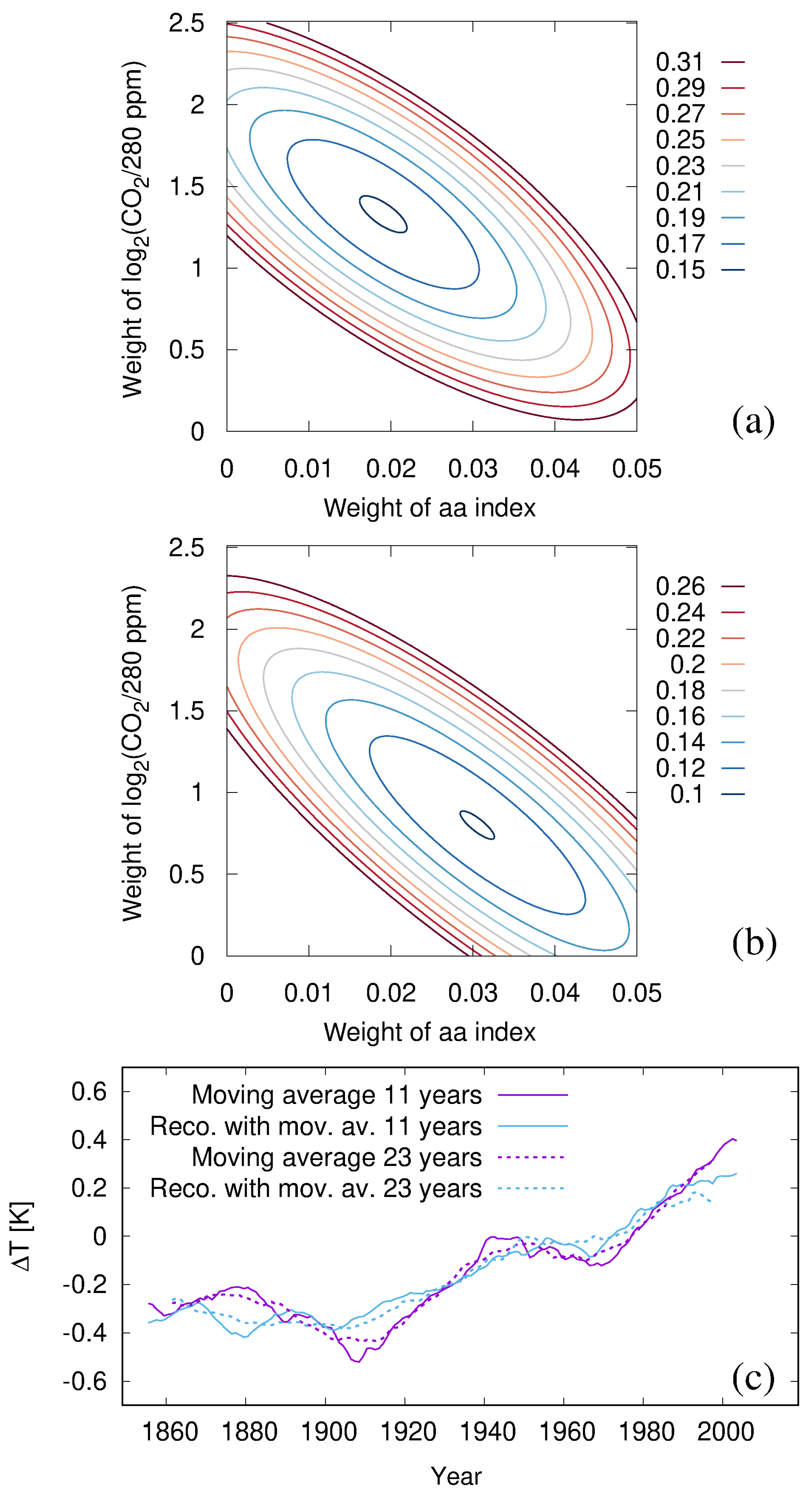
Let us start, however, with the full data ending in 2018. For the two MAW’s of 11 years and 23 years, Figure 4a,b shows the fraction of variance unexplained ($\mathrm{FVU}$), i.e., the ratio of the residual sum of squares to the total sum of squares, in dependence on the respective weights of the aa index ($w_{\mathrm{aa}}$, on the abscissa) and the logarithm of CO${}_2$ ($w_{{\mathrm{CO}}_2}$, on the ordinate axis). The latter value immediately provides us with a sort of instantaneous climate sensitivity of the TCR type. The minimum ${\mathrm{FVU}}_{\min }=0.107$ is obtained for the weights’ combination $w_{\mathrm{aa}}=0.011$ K/nT and $w_{{\mathrm{CO}}_2}=1.72$ K in the case of $\mathrm{MAW}=11$ years, and ${\mathrm{FVU}}_{\min }=0.102$ is obtained for $w_{\mathrm{aa}}=0.0162$ K/nT and $w_{{\mathrm{CO}}_2}=1.54$ K in the case of $\mathrm{MAW}=23$ years. From the ellipse-shaped contour plots of $\mathrm{FVU}$, we see that those minima reflect a dominating influence of CO${}_2$ over the aa index. The two red curves in Figure 4c now show the corresponding temperature reconstructions based on those optimized values of $w_{\mathrm{aa}}$ and $w_{{\mathrm{CO}}_2}$, for $\mathrm{MAW}=11$ years (full line) and for $\mathrm{MAW}=23$ years (dashed line). For both lines, we obtain a reasonable fit of the general upward trend of $\Delta T$, but a poor reconstruction of its oscillatory features. This clearly corresponds to the higher share of $w_{{\mathrm{CO}}_2}$ as compared to that of $w_{\mathrm{aa}}$. Any (tentative) higher share of $w_{\mathrm{aa}}$ would lead to a drastic decrease in the reconstructed $\Delta T$ for the last two decades, resulting in forbiddingly large $\mathrm{FVU}$ values when compared with the relatively high observed $\Delta T$ in this late period.

This brings us to the question of what happens if we exclude the latest “hot” 5 years (with their strong El Niño influence), thus restricting the date until 2013 only. The corresponding results are shown in Figure 5. Obviously, the optimal weights’ combination now shifts away from CO${}_2$ to $\mathrm{aa}$, with values $w_{\mathrm{aa}}=0.0145$ K/nT and $w_{{\mathrm{CO}}_2}=1.56$ K for $\mathrm{MAW}=11$ years and $w_{\mathrm{aa}}=0.0232$ K/nT and $w_{{\mathrm{CO}}_2}=1.21$ K for $\mathrm{MAW}=23$ years. Evidently, the resulting (green) temperature reconstruction curves in Figure 5c now appear more oscillatory.

In Figure 6, we show the corresponding plots for the case in which we select the end year 2008, which basically corresponds to the database of Mufti and Shah [46] (2007 in their case). Evidently, the regression for this shortened segment leads to a significantly stronger weight for the aa index. The minimum $\mathrm{FVU}$ is then obtained at $w_{\mathrm{aa}}=0.0190$ K/nT and $w_{{\mathrm{CO}}_2}=1.33$ K for $\mathrm{MAW}=11$ years, and at $w_{\mathrm{aa}}=0.0305$ K/nT and $w_{{\mathrm{CO}}_2}=0.80$ K for $\mathrm{MAW}=23$ years. Due to the dominance of $w_{\mathrm{aa}}$, the (blue) reconstruction curves in Figure 6c (in particular that for $\mathrm{MAW}=23$ years) now show a significant oscillatory behaviour.

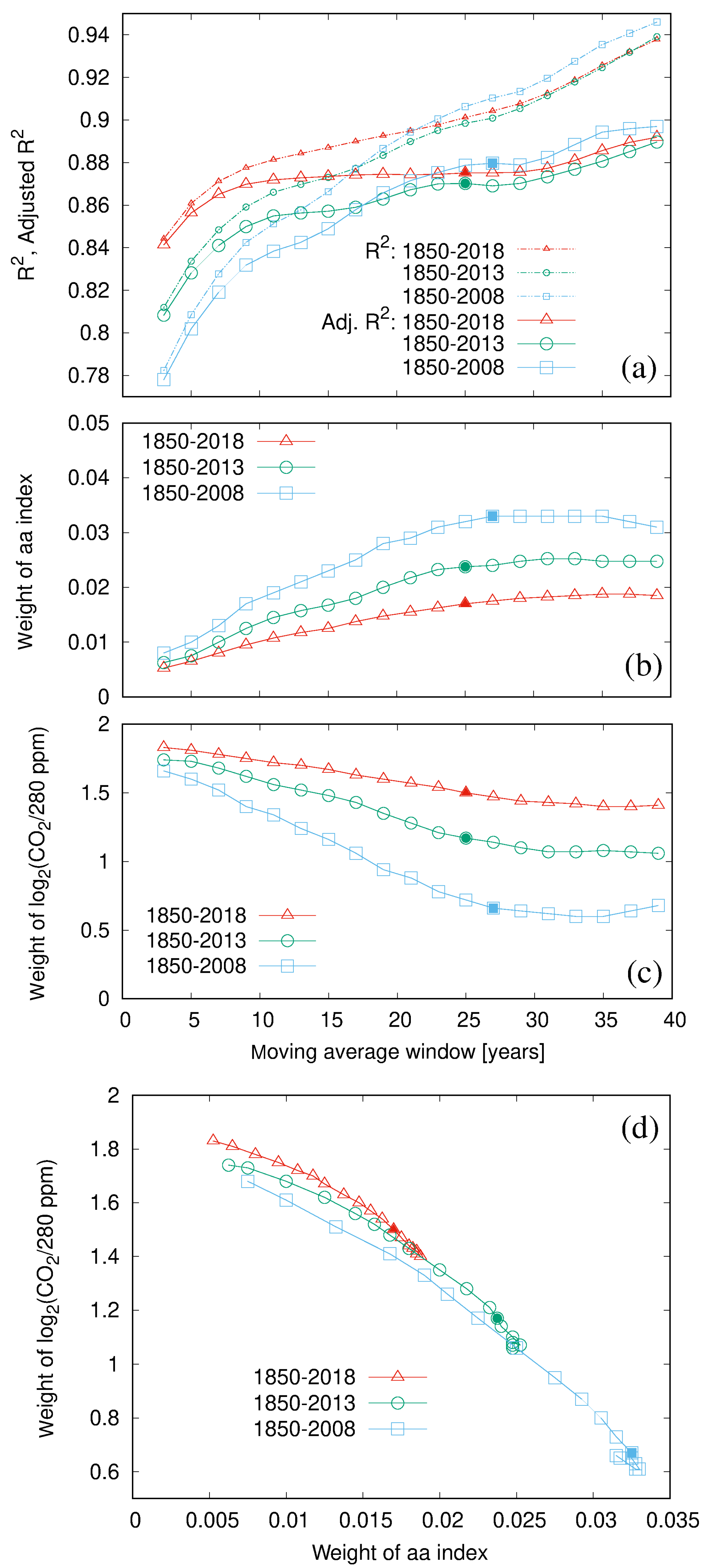
While those three examples provide a first illustration of how sensible the solution of the regression reacts on the choice of the end year, and the widths of the $\mathrm{MAW}$, the latter dependence is now studied in more detail. We first analyze the coefficient of determination $R^2$, which is related to the previously used $\mathrm{FVU}$ according to $R^2=1-\mathrm{FVU}$. The corresponding dashed curves in Figure 7a have a rather universal shape, starting from values of 0.78…0.84 for $\mathrm{MAW}=3$ years to around 0.94 for $\mathrm{MAW}=39$ years. The monotonic increase in $R^2$, which at first glance might suggest the use of high values of $\mathrm{MAW}$, has to be interpreted with caution. This has to do with the specific role of temporal averaging in our regression: a significant share of the increase in $R^2$ is just due to the increasing ratio of explanatory terms p (in our case two: $w_{\mathrm{aa}}$ and $w_{{\mathrm{CO}}_2}$) to the effective data number n. The latter is not identical to the number of considered years, $N_{\mathrm{y}}$, but—due to the moving average—approximately equal to $N_y/\mathrm{MAW}$. To correct for this effect, we use the so-called adjusted $R^2$, which is, in general, ${\overline{R}}^2=1-\mathrm{FVU}\times (n-1)/(n-p-1)$; hence, in our special case ${\overline{R}}^2=1-\mathrm{FVU}\times (N_y/\mathrm{MAW}-1)/(N_y/\mathrm{MAW}-3)$. This adjusted ${\overline{R}}^2$, as a much more telling coefficient of determination than $R^2$, is shown with full lines in Figure 7a. The monotonic increase still seen for $R^2$ now gives way to a more structured curve. For the green (data until 2013) and blue curves (data until 2008), we observe a local (if shallow) maximum around $\mathrm{MAW}=25$ years. The red curve (data until 2018) has a very flat plateau between $\mathrm{MAW}=11$ and $\mathrm{MAW}=27$ years, with an extremely shallow maximum at $\mathrm{MAW}=25$ years. We consider those local maxima around $\mathrm{MAW}=25$ years ($\mathrm{MAW}=27$ years for the blue curve) as a sort of best fit. Although ${\overline{R}}^2$ still rises slightly for the highest $\mathrm{MAW}$ values, the corresponding number of explained variables then becomes too small to allow for a decent reconstruction of the structure of the $\Delta T$ curve. As a side remark, while our methodology, with its focus on the adjusted $R^2$, is different from that of Love, Mursula and Tsai [48], the main results are not that dissimilar; using the lag-one auto-correlation $r^1$ (and a shorter time interval of 141 years), those authors had determined the effective data number of the aa index to either be 22 or 13 when using the annual data or the so-called first differences between cycle-averaged data, respectively (see their Table 1). The corresponding values for the temperature were indicated as eight and six, respectively, (and one might have guessed a similar number by a simple visual inspection of the zigzag curve in Figure 1a). This latter effective data number of six would, in their case, correspond to a MAW of 24 years, which is indeed encouragingly close to our optimum value of 25 years, obtained by considering the adjusted $R^2$, and also taking into account the CO${}_2$, which was not included in [48].

The corresponding dependencies for $w_{\mathrm{aa}}$ and $w_{{\mathrm{CO}}_2}$ are shown in Figure 7b,c, respectively. Figure 7d depicts the same solutions in the two-dimensional parameter space. In this representation, all three curves (red, green and blue) form a sort of common, weakly bent line, which appears to connect the extremal values of $w_{{\mathrm{CO}}_2}\approx 1.9$ K on the ordinate axis with $w_{\mathrm{aa}}\approx 0.04$ K/nT on the abscissa. This common line conflates the ellipsoidal shapes of the $\mathrm{FVU}$ as shown in Figure 3, Figure 4 and Figure 5 which, in turn, just reflected the significant ill-posedness of the underlying inverse problem. To put it differently: due to the high correlation coefficients of $\Delta T$, both with CO${}_2$ as well as with the aa index, the separate shares of the two ingredients are very hard to disentangle.

However questionable our fixation on the shallow maxima at $\mathrm{MAW}\approx 25$ years might ever be, Figure 7 also proves that any alternative choice of a higher $\mathrm{MAW}$ would not change the final solution drastically. In either case, both $w_{\mathrm{aa}}$ and $w_{{\mathrm{CO}}_2}$ would converge to a close-by value. Much more decisive is the distinction between the differently colored curves; for $w_{{\mathrm{CO}}_2}$, they give us results somewhere between 0.6 K and 1.6 K (in the latter case, we took into account the particular flatness of the maximum, which in reality might also lay at slightly lower values of $\mathrm{MAW}$).

In some sense, this is again a frustratingly wide range of values. As stated, it reflects the ill-posedness of the underlying inverse problem, whose non-uniqueness led to a high sensitivity on end effects related to the neglected factors, such as ENSO (and volcanic aerosols). Taking into account those short-term variations in the regression, as performed in [73,74], might have significantly sharpened the final outcome, but has to be left for future work. Complementary to that, the temperature development during the next decade(s) will also help; if it continues to grow, we will end up at the higher end of the $w_{{\mathrm{CO}}_2}$ range. In case of some imminent drop, it will point to lower values of $w_{{\mathrm{CO}}_2}$. At any rate, the decreasing correlation (i.e., multicollinearity) between $\mathrm{aa}$ (which is supposed to fall, or, at least, not rise significantly) and the (continuously rising) CO${}_2$ will more and more improve the quality of the regression analysis.

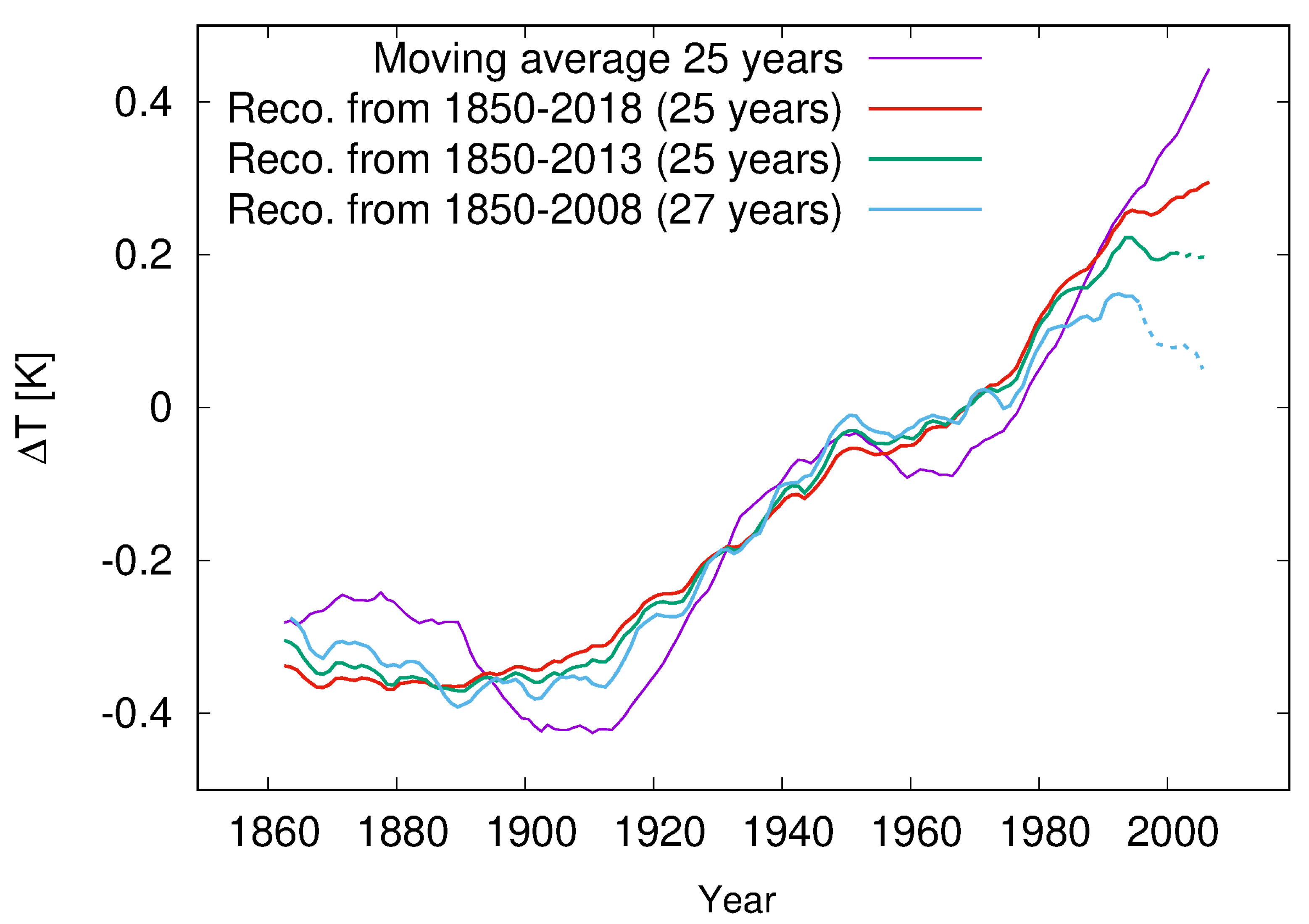
In Figure 8, we show all three temperature reconstructions with the optimal combinations of $w_{\mathrm{aa}}$ and $w_{{\mathrm{CO}}_2}$ as taken from Figure 7, together with the original $\Delta T$ data, averaged over 25 years. The dashed segments of the green and blue curves correspond to the later time segments which were deliberately omitted in the corresponding regression analysis. As expected, they exhibit an increasing divergence from the original $\Delta T$ data. On the other hand, from the red via the green to the blue curve, we also observe an improved reconstruction of the oscillatory behaviour of $\Delta T$. This is the crux of our problem; the better the reconstruction for the years until 1995, the larger is the deviation for the latest two decades. We will need approximately one decade of more data to be able to identify the best solution. For the green or blue lines to have any validity, a significant temperature drop in the nearest future will be unavoidable.

2.4. Some Plausibility Checks and Comparisons

Before entering the field of predictions, we would like to check the plausibility of the obtained estimates, in particular those at the lower end of the range. For that purpose, we shortly discuss the results of three papers, which were based on experimental and satellite-borne measurements.

Combining measurements at optically thick samples of CO${}_2$ with a five-layer numerical model for the greenhouse effect, Laubereau and Iglev [39] derived a temperature increase of 0.26 K for the 290 ppm to 385 ppm increase between 1880 and 2010, which resulted in a climate sensitivity of 0.636 K (per 2× CO${}_2$).

Feldman et al. [40] published results from two clear-sky surface radiative forcing measurements with the Atmospheric Emitted Radiance Interferometer (AERI) between 2000 and 2010, when the CO${}_2$ concentration increased (according to their estimate) by 22 ppm. They observed an increase of 0.2 W/m${}^2$ during this decade, which amounts to 2.4 W/m${}^2$ (per 2× CO${}_2$). With the usual zero-feedback sensitivity parameter of 0.27 K/(W/m${}^2$), this would translate into 0.65 K (per 2× CO${}_2$). If we were to use the modified value of 0.31 K/(W/m${}^2$) (which allows for variations with latitude [75]), we would obtain 0.75 K.

Later on, Rentsch [41] found a similar result by analyzing outgoing radiation under night-time, cloud-clear conditions. The CO${}_2$ rise from 373 ppm to 410 ppm led to a forcing of 0.358 W/m${}^2$, corresponding to 2.63 W/m${}^2$ (per 2× CO${}_2$), i.e., to 0.71 K (with 0.27 K/(W/m${}^2$)) or 0.82 K (with 0.31 K/(W/m${}^2$)), in nearly perfect agreement with Feldman et al. [40].

Hence, these three papers are mutually consistent, giving sensitivities in the range between 0.64 K and 0.82 K, which is close to the lower edge of our estimate. We also note that this end of our regression results, which corresponds to approximately 70 percent “for the sun”, is similar to the 50–69 percent range as once found by Scafetta [76,77].

That said, we also note that Wijngaarden and Happer [54] found the much higher value of 1.4 K (at fixed absolute humidity), which would fit to our upper limit of 1.6 K value, which is, in turn, significantly lower than their value 2.2–2.3 K, as inferred for fixed relative humidity.

The range of our estimates is slightly sharper than the range from 0.4 K to 2.5 K of Soon et al. [53] (with the high value deemed unrealistic by the authors), and slightly wider than the 0.8–1.3 K range of Lewis and Curry [52], but, in either case, quite consistent with those estimations.

3. Predictions

In the preceding Section, we have derived a certain plausible range of combinations of the respective weights of the aa index and the logarithm of CO${}_2$ by means of a regression analysis of data from the past 170 years. In the following, we leave the realm of solid, data-based science, and enter the more nebulous domain of predictions. Given all the underlying uncertainties concerning the future time dependence of the aa index, of CO${}_2$ and of further climate factors such as AMO, PDO, ENSO, volcanism, etc., any forecast has to be taken with a grain of salt. At least we will conduct some parameter studies, by allowing the unknown time series of the aa index and CO${}_2$, and their respective weights, to vary in some reasonable range. Let us start with the aa index.

3.1. Predicting the Solar Dynamo

This subsection is definitely the most speculative one of this paper, as it is concerned with forecasts of the aa index for the next 130 years. There is no doubt that the aa index is strongly correlated with the sunspot number (SSN), with typical correlation coefficients of around $r=0.96$ when averaged over one cycle [68]. Nor is there any doubt that the SSN and the aa index are both governed (though in a non-trivial manner) by the solar dynamo. Therefore, any prediction of the aa index boils down to a prediction of the solar dynamo, which many researchers believe to be impossible, at least beyond the horizon of the very next cycle, for which “precursor methods” exist [78,79,80] (although the underlying neural network methods might still learn from interesting applications in other fields [81]).

In order to justify our audacious forecast for the aa index, we have to make a little digression on the solar dynamo and its short-, medium- and long-term cycles. The reader should be warned, though, that our arguments do not reflect the mainstream of solar dynamo theory. We think, nevertheless, that the last years have brought about sufficient empirical evidence that warrants at least a cautious try.

Let us start with some recent evidence concerning the phase stability of the Schwabe cycle, a matter that was first discussed by Dicke [82]. In [61], we reviewed the pertinent results derived from algae data in the early Holocene [23] and from sunspot and aurorae borealis observations, combined with ${}^{14}$C and ${}^{10}$Be data, from the last centuries. Without going into the details, it was shown that the Schwabe cycle was very likely phase-stable at least over some centuries, with a period between 11.04 years and 11.07 years. While certain nonlinear self-synchronization mechanisms of the solar dynamo cannot be completely ruled out as an explanation [83], the external synchronization by the 11.07-year periodic spring tides of the (tidally dominant) Venus–Earth–Jupiter system provides a suspiciously compelling alternative. Based on previous observations and ideas [84,85,86,87,88], we corroborated a model [56,57,58,59,89], in which the weak tidal forces of Venus, Earth and Jupiter served only as an external trigger for synchronizing the intrinsic helicity oscillations of the kink-type Tayler instability in the tachocline region. The arising 11.07-year period of the helicity parameter $\alpha$ ultimately led to the 22.14-year period of the Hale cycle.

Building on this phase stability of the Hale cycle, in [60,62] we exploited ideas of Wilson [87] and Solheim [90] to explain the mid-term Suess-de Vries cycle as a beat period between the 22.14-year Hale cycle and the 19.86-year synodic cycle of Jupiter and Saturn, which governs the motion of the Sun around the barycenter of the solar system. Note that, apart from first ideas [87,90,91,92], the spin–orbit coupling that is necessary to translate the orbital motion of the Sun into some dynamo-relevant internal forcing, is yet far from understood. In our model, the Suess-de Vries cycle acquires a clear (beat) period of 193 years, which is in the lower range of usual estimates (see [93]). The situation with the Gleissberg cycle(s) was less clear; they appeared partly as double and triple overtones of the Suess-de Vries cycle, but also as independent frequencies resulting from beat periods of other synodic cycles of Jovian planets with the Schwabe cycle (see Figure 10 in [62]). Further below, this vagueness of the Gleissberg cycle(s) will be factored in when fitting and extrapolating the aa index. Lately, in [62], we tried to explain the transitions between regular and irregular intervals of the solar dynamo (the “supermodulation” as defined by Weiss and Tobias [63]) in terms of a transient route to chaos.

With these preliminaries, we now fit the aa index over the last 170 years in order to extrapolate it into the future. We assume that we have safely left the irregular period of the solar dynamo, as reflected in the Little Ice Age which can be considered as the latest link in the (chaotic) chain of Bond events [55]. Guided by our (double-)synchronization model, and encouraged by Ma and Vaquero [93], who had indeed derived a 195-year cycle in the quiet (regular) interval from 800 to 1340, we keep this Suess-de Vries period fixed to 193 years in all fits. Concerning the Gleissberg-type cycle(s), we are less strict. In the first version, we fix the two periods of 96 and 65 years; for the second one, we only fix the 96-year period, and for the third one, we keep both Gleissberg cycles undetermined.

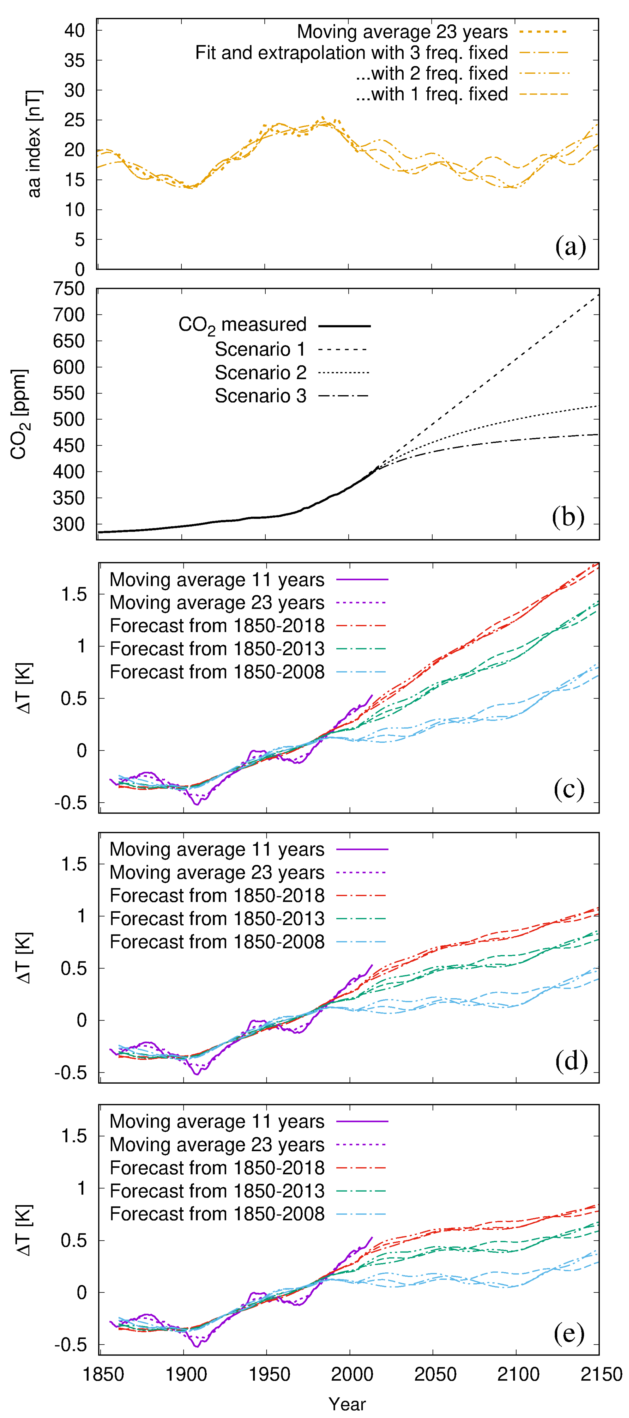
In the interval between 1850 and 2150, the results of these three different three-frequency fits are presented in Figure 9a, together with the (fitted) 23-year averaged aa index data between 1850 and 2007. Evidently, all three curves approximate the original data reasonably well, and all show a similar extrapolation with a long decay until 2100, and a recovery afterwards. This behavior is quite similar to the prediction of Bucha and Bucha [20] (their Figure 14), as well as with the variety of predictions in Reference [94]. The differences between the three fits mainly concern the high frequency part; whereas the version with three frequencies being fixed is the smoothest, the other two fits comprise some stronger wiggles. This simply reflects the fact that the Gleissberg cycle is more vague than the Suess-de Vries cycle. In the following, we will always work with all three curves obtained, hoping that they constitute a representative variety for the future of the aa index.

3.2. Some Scenarios

Thus prepared, we now consider three different CO${}_2$ scenarios (Figure 9b), for each of which we further take into account the three predictions for the aa index as just discussed, as well as the three optimal combinations of weights for the aa index and CO${}_2$ as derived in the previous section. Deliberately, we restrict our forecasts until 2150, admitting that neither the CO${}_2$ trend nor the aa index are seriously predictable beyond that horizon.

Let us start with the simple case (while we do not refer here to IPCC’s Representative Concentration Pathways, this case has some similarity to their RCP 6.0, at least until 2100.) of an unabated linear extrapolation of the recent CO${}_2$ trend to rise by 2.5 ppm annually (upper curve in Figure 9b), which would bring us to a value of 736 ppm in 2150 (still steeper trends are not completely ruled out, but perhaps not that realistic, given the recent worldwide reduction commitments). For this scenario, Figure 9c shows three red, green and blue bundles of curves, each comprising the three different fits of the aa index as discussed above. The red bundle (“hot”) corresponds to the red solution in Figure 7, with a rather high CO${}_2$-sensitivity of 1.5 K and an aa sensitivity of 0.017 K/nT. The green bundle (“medium”) corresponds to the green solution of Figure 7 based on sensitivities of 1.2 K and 0.022 K/nT. The blue bundle (“cool”) corresponds to 0.6 K and 0.032 K/nT.

We see that, in 2100, the “hot” variant leads to a temperature anomaly of $\Delta T=1.3$ K, which is $0.9$ K above the average $\Delta T\approx 0.4$ K from the first decade of this century. Such an increase would be quite compatible with the prediction of Scafetta [74]. Our “medium” and “cool” curves are flatter, leading to $\Delta T=0.9$ K and $\Delta T=0.4$ K, respectively. However, for those cases to be of any relevance, an imminent drop of temperature would be required before the corresponding curves could continue as flat as shown. In either case, the variation of the temperature predictions between the three different fits of the aa index is in the range of 0.1 K, which is much smaller than the respective differences between the “hot”, “medium” and “cool” curve bundles.

The second scenario (dotted line in Figure 9b) assumes a slowly decreasing upward trend of the CO${}_2$ concentration towards the end of the 21st century, with a hypothetical time dependence

$${\mathrm{CO}}_2=[382+2.5(t-2007)/(1.+(t-2007)/100)]\mathrm{ppm}$$

reaching a final value of 529 ppm in 2150. The resulting red, green and blue curves in Figure 9d show a rather flat behavior.

The last (and rather unrealistic) CO${}_2$ scenario (dash-dotted line of Figure 9b) assumes a radical decarbonization path with

$${\mathrm{CO}}_2=[382+2.5(t-2007)/(1.+(t-2007)/50)]\mathrm{ppm}.$$

The resulting temperature curves (Figure 7e) are basically constant throughout the end of our forecast horizon.

4. Summary and Discussion

This work has revived the tradition of correlating solar magnetic field data with the terrestrial climate as pioneered by Cliver et al. [45] and Mufti and Shah [46]. Just as these authors, we found an empirical correlation coefficient between the aa index and $\Delta T$ with remarkably high values ranging from 0.8 to 0.96, which points to a significant influence of solar variability on the climate. Our modest innovation was to employ a double regression analysis, with the logarithm of the atmospheric CO${}_2$ concentration as the second independent variable, whose pre-factor corresponds to an (instantaneous) climate sensitivity of the TCR type. For the lengths of the centered moving average window of 25 years, we identified optimal parameter combinations leading to adjusted $R^2$ values of around 87 percent. Depending on whether to include or not include the data from the last decade, the regression gave climate sensitivity values from 1.6 K down to 0.6 K (per $2\times$ CO${}_2$), and values from 0.017 K/nT up to 0.032 K/nT for the corresponding sensitivity on the aa index.

Ironically, if interpreted as $1.1\pm 0.5$ K, the derived climate sensitivity range turns out to have (nearly) the same ample 50 percent error bar as the “official” ECS value ($3\pm 1.5$ K), which we had criticized in the introduction. Yet, in view of the impressive 95 percent correlation (obtained for the restricted period 1850–2008), we believe the correct climate sensitivity to be situated somewhere in the lower half of that range. This “bias” is also supported by the fact that, during the last years, an intervening strong El Niño, a positive PDO (prevailing between 2014 and 2016), and a positive AMO, all conspired to raise the temperature to significantly higher values than what would be expected from the sole combination of the aa index and CO${}_2$. With the upcoming switch to La Niña conditions, and the imminent return of the PDO and AMO into their negative phases, we expect a significant temperature drop for the coming years, which might then re-establish the strong correlation between $\Delta T$ and the aa index (it remains to be seen whether the plummeting temperatures observed from December 2020 to June 2021 were already the harbinger of a more robust downward trend, or just a fluctuation due to intermediate La Niña conditions). We should also mention the theoretical possibility that the (supposedly independent) ENSO variability is, in itself, a function of the average temperature [95]. In this case, our linear ansatz, and the underlying distinction between short-term and long-term effects, would become increasingly problematic. At any rate, the next decade will be decisive for distinguishing between climate sensitivity values in the lower versus those in the upper half of the derived range. In this sense we are more optimistic than Love et al. [48], who believed that we “…would have to patiently wait for decades before enough data could be collected to provide meaningful tests…”. Given the high correlation for most of the past 170 years, and the good correspondence with the results of recent satellite-borne measurements [40,41], our “bets” are clearly on the lower half of that range.

Based on those estimates, we presented some cautious climate predictions for the next 130 years. With the derived share of the solar influence reaching values between 30 and 70 percent, such predictions depend critically on a correct forecast of the solar dynamo (in addition to that of CO${}_2$, of course). Following our recent work towards a self-consistent planetary synchronization model of short- and medium-term cycles of the solar dynamo, we extrapolated some simple three-frequency fits of the aa index to the data from the last 170 years into the next 130 years. Apart from intrinsic variabilities of such forecasts (mainly connected with the vagueness of the Gleissberg-type cycle(s)), we prognosticated a general decline of the aa index until 2100, which essentially reflects the 200-year Suess-de Vries cycle. Such a prediction presupposes that we indeed have left the irregular solar dynamo episode (corresponding to the Little Ice Age, the latest “Bond event”) and that we will further remain in a regular phase of solar activity [62,63], similar to that between 800 and 1340 [93]. Of course, we have to ask ourselves whether our prediction of a declining aa index could be completely wrong, with the Sun eventually becoming even “hotter” in the future, thus adding to the warming of CO${}_2$. While such a scenario could not be completely ruled out, we consider it as not very likely, given that the solar activity at the end of the 20th century was perhaps the highest during the last 8000 years [96], and that it has declined ever since.

As for the CO${}_2$ trend, we examined three scenarios, comprising an unfettered 2.5 ppm annual increase until 2150, as well as one soft and one radical decarbonization scheme. Even in the “hottest” case considered, we only found a mild additional temperature rise of less than 1 K until the end of this century, while all other cases resulted in flatter curves in which the heating effect of increasing CO${}_2$ was widely compensated for by the cooling effect of a decreasing aa index. Hence, the advocated 2 K goal could likely be met even without any drastic decarbonization measures. Apart from that, we also advise that any imminent temperature drop (due to the turn of ENSO, PDO and AMO into their respective negative phases) should not be mistaken as, and extrapolated to, a long-lasting downward trend [97].

5. Conclusions and Outlook

In this work, we focused exclusively on a quasi-instantaneous, i.e., TCR-like, climate sensitivity on CO${}_2$. As for ECS, we agree with Knutti et al. [3], who opined that “(k)nowing a fully equilibrated response is of limited value for near-term projections and mitigation decisions” and that “(t)he TCR is more relevant for predicting climate change over the next century”. In view of the millennial relaxation time scale underlying the concept of ECS, we caution that any intervening grand minimum of the solar dynamo would undermine the predictive power of our model. Moreover, we fear that the huge Milankovitch drivers [98] will—perhaps much too soon—massively interfere with the solar and anthropogenic factors that were considered in this paper.

References

1. Arrhenius, S. Die vermutliche Ursache der Klimaschwankungen. Medd. Kungl. Vetenskpasakad. Nobelinst. 1906, 1, 1–10. [Google Scholar]
2. Callendar, G.S. The artificial production of carbon dioxide and its influence on temperature. Q. J. R. Meteorol. Soc. 1938, 64, 223–240. [Google Scholar] [CrossRef]
3. Knutti, R.; Rugenstein, M.A.A.; Hegerl, G.C. Beyond equilibrium climate sensitivity. Nat. Geosci. 2017, 10, 727–736. [Google Scholar] [CrossRef]
4. Charney, J.G.; Arakawa, A.; Baker, D.J.; Bolin, B.; Dickinson, R.E.; Goody, R.M.; Leith, C.E.; Stommel, H.M.; Wunsch, C.I. Carbon Dioxide and Climate: A Scientific Assessment; National Academy of Sciences Press: Washington, DC, USA, 1979. [Google Scholar]
5. Lindzen, R.S. An oversimplified picture of the climate behavior based on a single process can lead to distorted conclusions. Eur. Phys. J. Plus 2020, 135, 462. [Google Scholar] [CrossRef]
6. Vahrenholt, F.; Lüning, S. Unerwünschte Wahrheiten: Was Sie über den Klimawandel Wissen Sollten; Langen-Müller: Munich, Germany, 2020. [Google Scholar]
7. Hoyt, D.V.; Schatten, K.H. A discussion of plausible solar irradiance variations. J. Geophys. Res. 1993, 98, 18895–18906. [Google Scholar] [CrossRef] [Green Version]
8. Gray, L.J.; Beer, J.; Geller, M.; Haigh, J.D.; Lockwood, M.; Matthes, K.; Cubasch, U.; Fleitmann, D.; Harrison, G.; Hood, L.; et al. Solar influence on climate. Rev. Geophys. 2010, 48, 1–53. [Google Scholar] [CrossRef]
9. Lean, J.L. Cycles and trends in solar irradiance and climate? WIREs Clim. Chang. 2010, 1, 111–121. [Google Scholar] [CrossRef]
10. Labitzke, K.; van Loon, H. Associations between the 11-year solar cycle, the QBO and the atmosphere. Part 1: The troposphere and stratosphere in the northern hemisphere in winter. J. Atmos. Terr. Phys. 1988, 50, 197–206. [Google Scholar] [CrossRef]
11. Haigh, J.D. The role of stratospheric Ozon in modulating the solar radiative forcing of climate. Nature 1994, 370, 544–546. [Google Scholar] [CrossRef]
12. Soon, W.H.; Posmentier, E.S.; Baliunas, S.L. Climate hypersensitivity to solar forcing? Ann. Geophys. 2000, 18, 583–588. [Google Scholar] [CrossRef]
13. Georgieva, K.; Kirov, B.; Koucka Knizova, P.; Mosna, Z.; Kouba, D.; Asenovska, Y. Solar influence on atmospheric circulation. J. Atmos. Sol.-Terr. Phys. 2012, 90–91, 15–21. [Google Scholar] [CrossRef]
14. Silverman, V.; Harnik, N.; Matthes, K.; Lubis, S.W.; Wahl, S. Radiative effects of ozone waves on the Northern Hemisphere polar vortex and its modulation by the QBO. Atmos. Chem. Phys. 2018, 18, 6637–6659. [Google Scholar] [CrossRef] [Green Version]
15. Veretenenko, S.; Ogurtsov, M.G. Influence of Solar-geophysical factors on the state of the stratospheric polar vortex. Geomagn. Aeron. 2020, 60, 974–981. [Google Scholar] [CrossRef]
16. Svensmark, H.; Friis-Christensen, E. Variations of cosmic ray flux and global cloud coverage—A missing link in solar-climate relationship. J. Atmos. Sol.-Terr. Phys. 1997, 59, 1225–1232. [Google Scholar] [CrossRef]
17. Soon, W.H.; Baliunas, S.L.; Posmentier, E.S.; Okeke, P. Variations of solar coronal hole area and terrestrial lower tropospheric air temperature from 1979 to mid-1998: Astronomical forcings of change in earth’s climate? New Astron. 2000, 4, 563–579. [Google Scholar] [CrossRef]
18. Shaviv, N.J.; Veizer, J. Celestial driver of Phanerozoic climate? GSA Today 2003, 13, 4–10. [Google Scholar] [CrossRef]
19. Svensmark, H.; Enghoff, M.B.; Shaviv, N.J.; Svensmark, J. Increased ionization supports growth of aerosols into cloud condensation nuclei. Nat. Commun. 2017, 8, 2199. [Google Scholar] [CrossRef] [Green Version]
20. Bucha, V.; Bucha, V., Jr. Geomagnetic forcing of changes in climate and in the atmospheric circulation. J. Atmos. Sol.-Terr. Phys. 1998, 60, 145–169. [Google Scholar] [CrossRef]
21. Tinsley, B.A. Influence of solar wind on the global electric current, and inferred effects on cloud microphysics, temperature, and dynamics in the troposphere. Space Sci. Rev. 2000, 94, 231–258. [Google Scholar] [CrossRef]
22. Tinsley, B.A. The global atmospheric electric circuit and its effects on cloud microphysics. Rep. Prog. Phys. 2008, 71, 66801–66900. [Google Scholar] [CrossRef]
23. Vos, H.; Brüchmann, C.; Lücke, A.; Negendank, J.F.W.; Schleser, G.H.; Zolitschka, B. Phase Stability of the Solar Schwabe Cycle in Lake Holzmaar, Germany, and GISP2, Greenland, between 10,000 and 9000 cal. BP. In Climate in Historical Times: Towards a Synthesis of Holocene Proxy Data and Climate Models, GKSS School of Environmental Research; Fischer, H., Kumke, T., Lohmann, G., Floser, G., Miller, H., Storch, H., Eds.; Springer: Berlin/Heidelberg, Germany, 2004; pp. 293–317. [Google Scholar]
24. Charlson, R.J.; Lovelock, J.E.; Andreae, M.O.; Warren, S.C. Oceanic phytoplankton, atmospheric sulphur, cloud albedo and climate. Nature 1987, 326, 655–661. [Google Scholar] [CrossRef]
25. Scafetta, N.; Willson, R.C. ACRIM total solar irradiance satellite composite validation versus TSI proxy models. Astrophys. Space Sci. 2014, 350, 421–442. [Google Scholar] [CrossRef] [Green Version]
26. Egorova, T.; Schmutz, W.; Rozanov, E.; Shapiro, A.I.; Usoskin, I.; Beer, J.; Tagirov, R.V.; Peter, T. Revised historical solar irradiance forcing. Astron. Astrophys. 2018, 615, A85. [Google Scholar] [CrossRef] [Green Version]
27. Connolly, R.; Soon, W.; Connolly, M.; Baliunas, S.; Berglund, J.; Butler, C.J.; Cionco, R.G.; Elias, A.G.; Fedorov, V.M.; Harde, H.; et al. How much has the Sun influence Northern hemisphere temperature trends. An ongoing debate. Res. Astron. Astrophys. 2021, 21, 131. [Google Scholar] [CrossRef]
28. Wang, Y.-M.; Lean, J.L.; Sheeley, N.R., Jr. Modelling the Sun’s magnetic field and irradiance since 1713. Astrophys. J. 2009, 625, 522–538. [Google Scholar] [CrossRef]
29. Steinhilber, F.; Beer, J.; Fröhlich, C. Total solar irradiance during the Holocene. Geophys. Res. Lett. 2009, 36, L19704. [Google Scholar] [CrossRef] [Green Version]
30. Krivova, N.A.; Vieira, L.E.A.; Solanki, S. Reconstruction of solar spectral irradiance since the Maunder minimum. J. Geophys. Res. Space Phys. 2010, 115, A12112. [Google Scholar] [CrossRef] [Green Version]
31. Solanki, S.K. Solar variability and climate change: Is there a link? Astron. Geophys. 2002, 43, 5.9–5.13. [Google Scholar] [CrossRef] [Green Version]
32. Courtillot, V.; Gallet, Y.; Le Mouël, J.-L.; Fluteau, F.; Genevey, A. Are there connections between the Earth’s magnetic field and climate? Earth Planet. Sci. Lett. 2007, 253, 328–339. [Google Scholar] [CrossRef]
33. Bindoff, N.L.; Stott, P.A.; Achuta Rao, K.M.; Allen, M.R.; Gillett, N.; Gutzler, D.; Hansingo, K.; Hegerl, G.; Hu, Y.; Jain, S.; et al. Detection and Attribution of Climate Change: From Global to Regional. In IPCC AR5 WG1 Ch10; Cambridge University Press: Cambridge, UK; New York, NY, USA, 2013. [Google Scholar]
34. Wyatt, M.G.; Peters, J.M. A secularly varying hemispheric climate-signal propagation previously detected in instrumental and proxy data not detected in CMIP3 data base. SpringerPlus 2012, 1, 68. [Google Scholar] [CrossRef] [Green Version]
35. Pinault, J.-L. Resonant forcing of the climate system in subharmonic modes. J. Mar. Sci. Eng. 2020, 8, 60. [Google Scholar] [CrossRef] [Green Version]
36. Pinault, J.-L. Resonantly forced baroclinic waves in the oceans: A new approach to climate variability. J. Mar. Sci. Eng. 2021, 9, 13. [Google Scholar] [CrossRef]
37. Cook, J.; Oreskes, N.; Doran, P.T.; Anderegg, W.R.L.; Verheggen, B.; Maibach, E.W.; Carlton, J.S.; Lewandowsky, S.; Skuce, A.G.; Green, S.E.; et al. Consensus on consensus: A synthesis of consensus estimates on human-caused global warming. Environ. Res. Lett. 2016, 11, 048002. [Google Scholar] [CrossRef]
38. Parker, E.N. Sunny side of global warming. Nature 1999, 399, 416–417. [Google Scholar] [CrossRef]
39. Laubereau, A.; Iglev, H. On the direct impact of the CO2 concentration rise to the global warming. EPL 2013, 104, 29001. [Google Scholar] [CrossRef]
40. Feldman, D.R.; Collins, W.D.; Gero, P.J.; Torn, M.S.; Mlawer, E.J.; Shipper, T.R. Observational determination of surfaced radiative forcing by CO2 from 2000 to 2010. Nature 2015, 519, 339–343. [Google Scholar] [CrossRef] [Green Version]
41. Rentsch, C.P. Radiative forcing by CO2 observed at top of atmosphere from 2002 to 2019. arXiv 2019, arXiv:1911.10605. [Google Scholar]
42. Reid, G. Influence of solar variability on global sea surface temperatures. Nature 1987, 329, 142–143. [Google Scholar] [CrossRef]
43. Friis-Christensen, E.; Lassen, K. Length of the solar cycle: An indicator of solar activity closely associated with climate. Science 1991, 254, 698–700. [Google Scholar] [CrossRef] [Green Version]
44. Solheim, J.-E.; Stordahl, K.; Humlum, O. The long sunspot cycle 23 predicts a significant temperature decrease in cycle 24. J. Atmos. Sol.-Terr. Phys. 2012, 80, 267–284. [Google Scholar] [CrossRef] [Green Version]
45. Cliver, C.W.; Boriakoff, V.; Feynman, J. Solar variability and climate change: Geomagnetic aa index and global surface temperature. Geophys. Res. Lett. 1998, 25, 1035–1038. [Google Scholar] [CrossRef] [Green Version]
46. Mufti, S.; Shah, G.N. Solar-geomagnetic activity influence on Earth’s climate. J. Atmos. Sol.-Terr. Phys. 2011, 73, 1607–1615. [Google Scholar] [CrossRef]
47. Mayaud, P.-N. The aa indices: A 100-year series characterizing the magnetic activity. J. Geophys. Res. 1972, 77, 6870–6874. [Google Scholar] [CrossRef]
48. Love, J.J.; Mursula, K.; Tsai, V.C.; Perkins, D.M. Are secular correlations between sunspots, geomagnetic activity, and global temperature significant? Geophys. Res. Lett. 2012, 38, L21703. [Google Scholar] [CrossRef] [Green Version]
49. Pulkkinen, T.I.; Nevanlinna, H.; Pulkkinen, P.J.; Lockwood, M. The Sun-Earth connection in time scales from years to decades and centuries. Space Sci. Rev. 2001, 95, 625–637. [Google Scholar] [CrossRef]
50. Zherebtsov, G.A.; Kovalenko, V.A.; Molodykh, S.I.; Kirichenko, K.E. Solar variability manifestations in weather and climate characteristics. J. Atmos. Sol.-Terr. Phys. 2019, 182, 217–222. [Google Scholar] [CrossRef]
51. Soon, W.H.; Posmentier, E.S.; Baliunas, S.L. Inference of solar irradiance variability from terrestrial temperature changes, 1880–1993: An astrophysical application of the Sun-climate connection. Astrophys. J. 1996, 472, 891–902. [Google Scholar] [CrossRef] [Green Version]
52. Lewis, N.; Curry, J. The Impact of Recent Forcing and Ocean Heat Uptake Data on Estimates of Climate Sensitivity. J. Clim. 2018, 31, 6051–6071. [Google Scholar] [CrossRef]
53. Soon, W.; Conolly, R.; Conolly, M. Re-evaluating the role of solar variability on Northern Hemisphere temperature trends since the 19th century. Earth Sci. Rev. 2015, 150, 409–452. [Google Scholar] [CrossRef]
54. van Wijngaarden, W.A.; Happer, W. Dependence of Earth’s Thermal Radiation on Five Most Abundant Greenhouse Gases. arXiv 2020, arXiv:2006.03098. [Google Scholar]
55. Bond, G.; Kromer, B.; Beer, J.; Muscheler, R.; Evans, M.N.; Showers, W.; Hoffmann, S.; Lotti-Bond, R.; Hajdas, I.; Bonani, G. Persistent solar influence on North Atlantic climate during the Holocene. Science 2001, 294, 2130–2136. [Google Scholar] [CrossRef] [PubMed] [Green Version]
56. Stefani, F.; Giesecke, A.; Weber, N.; Weier, T. Synchronized helicity oscillations: A link between planetary tides and the solar cycle? Sol. Phys. 2016, 291, 2197–2212. [Google Scholar] [CrossRef]
57. Stefani, F.; Galindo, V.; Giesecke, A.; Weber, N.; Weier, T. The Tayler instability at low magnetic Prandtl numbers: Chiral symmetry breaking and synchronizable helicity oscillations. Magnetohydrodynamics 2017, 53, 169–178. [Google Scholar] [CrossRef]
58. Stefani, F.; Giesecke, A.; Weber, N.; Weier, T. On the synchronizability of Tayler-Spruit and Babcock-Leighton type dynamos. Sol. Phys. 2018, 293, 12. [Google Scholar] [CrossRef] [Green Version]
59. Stefani, F.; Giesecke, A.; Weier, T. A model of a tidally synchronized solar dynamo. Sol. Phys. 2019, 294, 60. [Google Scholar] [CrossRef] [Green Version]
60. Stefani, F.; Giesecke, A.; Seilmayer, M.; Stepanov, R.; Weier, T. Schwabe, Gleissberg, Suess-de Vries: Towards a consistent model of planetary synchronization of solar cycles. Magnetohydrodynamics 2020, 56, 269–280. [Google Scholar]
61. Stefani, F.; Beer, J.; Giesecke, A.; Gloaguen, T.; Seilmayer, M.; Stepanov, R.; Weier, T. Phase coherence and phase jumps in the Schwabe cycle. Astron. Nachr. 2020, 341, 600–615. [Google Scholar] [CrossRef]
62. Stefani, F.; Stepanov, R.; Weier, T. Shaken and stirred: When Bond meets Suess-de Vries and Gnevyshev-Ohl. Sol. Phys. 2021, 296, 88. [Google Scholar] [CrossRef]
63. Weiss, N.O.; Tobias, S.M. Supermodulation of the Sun’s magnetic activity: The effects of symmetry changes. Mon. Not. Roy. Astron. Soc. 2016, 456, 2654–2661. [Google Scholar] [CrossRef]
64. Kennedy, J.J.; Rayner, N.A.; Atkinson, C.P.; Killick, R.E. An ensemble data set of sea surface temperature change from 1850: The Met Office Hadley Centre HadSST.4.0.0.0 data set. J. Geophys. Res. Atmos. 2019, 124, 7719–7763. [Google Scholar] [CrossRef]
65. Sutton, R.T.; Dong, B.; Gregory, J.M. Land/sea warming ratio in response to climate change: IPCC AR4 model results and comparison with observations. Geophys. Res. Lett. 2007, 34, L02701. [Google Scholar] [CrossRef]
66. Scafetta, N. Detection of non-climatic biases in land surface temperature records by comparing climatic data and their model simulations. Clim. Dyn. 2021, 56, 2959–2982. [Google Scholar] [CrossRef]
67. Clilverd, M.A.; Clark, T.D.G.; Clarke, E.; Rishbeth, H. Increased magnetic storm activity from 1868 to 1995. J. Atm. Sol.-Terr. Phys. 1998, 60, 1047–1056. [Google Scholar] [CrossRef]
68. Cliver, C.W.; Boriakoff, V.; Bounar, K.H. Geomagnetic activity and the solar wind during the Maunder Minimum. Geophys. Res. Lett. 1998, 25, 897–900. [Google Scholar] [CrossRef]
69. Nevanlinna, H.; Kataja, E. An extension of the geomagnetic activity index series aa for two solar cycles (1844–1868). Geophys. Res. Lett. 1993, 20, 2703–2706. [Google Scholar] [CrossRef]
70. Mantua, N.J.; Hare, S.R. The Pacific Decadal Oscillation. J. Oceanography 2002, 58, 35–44. [Google Scholar] [CrossRef]
71. Wyatt, M.G.; Kravtsov, S.; Tsonis, A.A. Atlantic Multidecadal Oscillation and Northern Hemisphere is climate variability. Clim. Dyn. 2012, 38, 929–949. [Google Scholar] [CrossRef]
72. Roy, I.; Asikainen, T.; Maliniemi, V.; Mursula, K. Comparing the influence of sunspot activity and geomagnetic activity on winter surface climate. J. Atmos. Sol.-Terr. Phys. 2016, 149, 167–179. [Google Scholar] [CrossRef]
73. Lean, J.L.; Rind, D.H. How natural and anthropogenic influences alter global and regional surface temperatures: 1889 to 2006. Geophys. Res. Lett. 2008, 35, L18701. [Google Scholar] [CrossRef] [Green Version]
74. Scafetta, N. Reconstruction of the interannual to millennial scale patterns of the global surface temperature. Atmosphere 2021, 12, 147. [Google Scholar] [CrossRef]
75. Soden, B.J.; Held, I.M. An assessment of climate feedbacks in coupled ocean-atmosphere models. J. Clim. 2006, 19, 3354–3360. [Google Scholar] [CrossRef]
76. Scafetta, N.; West, I.M. Phenomenological reconstructions of the solar signature in the Northern Hemisphere surface temperature records since 1600. J. Geophys. Res. Atmos. 2007, 112, D24S03. [Google Scholar] [CrossRef] [Green Version]
77. Scafetta, N.; West, I.M. Is climate sensitive to solar variability. Phys. Today 2008, 61, 50–51. [Google Scholar] [CrossRef] [Green Version]
78. Svalgaard, L.; Cliver, E.W.; Kamide, Y. Sunspot cycle 24: Smallest cycle in 100 years? Geophys. Res. Lett. 2005, 32, L01104. [Google Scholar] [CrossRef] [Green Version]
79. Petrovay, K. Solar cycle prediction. Liv. Rev. Sol. Phys. 2020, 17, 2. [Google Scholar] [CrossRef] [Green Version]
80. Velasco Herrera, V.M.; Soon, W.; Legates, D.R. Does machine learning reconstruct missing sunspots and forecast a new solar minimum? J. Atmos. Sol.-Terr. Phys. 2019, 184, 57–62. [Google Scholar]
81. Chattopadhyay, G.; Midya, S.K.; Chattopadhyay, S. MLP based predictive model for surface ozone concentration over an urban area in the Gangetic West Bengal during pre-monsoon season. Adv. Space Res. 2021, 68, 1485–1501. [Google Scholar] [CrossRef]
82. Dicke, R.H. Is there a chronometer hidden deep in the Sun? Nature 1978, 276, 676–680. [Google Scholar] [CrossRef]
83. Hoyng, P. Is the solar cycle timed by a clock? Solar Phys. 1996, 169, 253–264. [Google Scholar] [CrossRef]
84. Hung, C.-C. Apparent relations between solar activity and solar tides caused by the planets. In NASA/TM–2007-214817; Glenn Research Center: Cleveland, OH, USA, 2007. [Google Scholar]
85. Wilson, I.R.G.; Carter, B.D.; Waite, I.A. Does a spin–orbit coupling between the Sun and the Jovian planets govern the solar cycle? Publ. Astron. Soc. Austr. 2008, 25, 85–93. [Google Scholar] [CrossRef] [Green Version]
86. Scafetta, N. Does the Sun work as a nuclear fusion amplifier of planetary tidal forcing? A proposal for a physical mechanism based on the mass-luminosity relation. J. Atmos. Sol.-Terr. Phys. 2012, 81–82, 27–40. [Google Scholar] [CrossRef] [Green Version]
87. Wilson, I.R.G. The Venus-Earth-Jupiter spin–orbit coupling model. Pattern Recogn. Phys. 2013, 1, 147–158. [Google Scholar] [CrossRef] [Green Version]
88. Okhlopkov, V.P. The gravitational influence of Venus, the Earth, and Jupiter on the 11-year cycle of solar activity. Mosc. Univ. Phys. Bull. 2016, 71, 440–446. [Google Scholar] [CrossRef]
89. Weber, N.; Galindo, V.; Stefani, F.; Weier, T. The Tayler instability at low magnetic Prandtl numbers: Between chiral symmetry breaking and helicity oscillations. New J. Phys. 2015, 17, 113013. [Google Scholar] [CrossRef]
90. Solheim, J.-E. The sunspot cycle length-modulated by planets? Pattern Recogn. Phys. 2013, 1, 159–164. [Google Scholar] [CrossRef]
91. Javaraiah, J. Long-Term Variations in the Solar Differential Rotation. Solar Phys. 2003, 212, 23–49. [Google Scholar] [CrossRef]
92. Sharp, G. Are Uranus and Neptune responsible for solar grand minima and solar cycle modulation? Int J. Astron. Astrophys. 2013, 3, 260–273. [Google Scholar] [CrossRef] [Green Version]
93. Ma, L.; Vaquero, J.M. New evidence of the Suess/de Vries cycle existing in historical naked-eye observations of sunspots. Open Astron. 2020, 29, 28–31. [Google Scholar] [CrossRef]
94. Lüdecke, H.-J.; Weiss, C.O.; Hempelmann, A. Paleoclimate forcing by the solar De Vries/Suess cycle. Clim. Past Discuss. 2015, 11, 279–305. [Google Scholar]
95. Fredriksen, H.-B.; Berner, J.; Subramanian, A.C.; Capotondi, A. How does El Niño-Southern Oscillation change under global warming—A first look at CMIP6. Geophys. Res. Lett. 2020, 47, e2020GL090640. [Google Scholar] [CrossRef]
96. Solanki, S.K.; Usoskin, I.G.; Kromer, B.; Schüssler, M.; Beer, J. Unusual activity of the Sun during recent decades compared to the previous 11,000 years. Nature 2004, 431, 1084–1087. [Google Scholar] [CrossRef] [PubMed] [Green Version]
97. Abdussamatov, H. Current long-term negative average annual energy balance of the Earth leads to the new little ice age. Thermal Sci. 2015, 19 (Suppl. S2), 279–288. [Google Scholar] [CrossRef]
98. Roe, G. In defense of Milankovitch. Geophys. Res. Lett. 2006, 33, L24703. [Google Scholar] [CrossRef] [Green Version]
Figure 1. Data of the HadSST sea surface temperature anomaly Δ T (a), the aa index (b) and log 2 of the ratio of the CO 2 concentration to the reference value of 280 ppm (c). The annual data between 1850 and 2018 are complemented by centered moving averages with windows 11 years and 23 years, as also utilized by Mufti and Shah [46]. The sources of the data are described in the text.
Climate 09 00163 g001
Figure 2. Comparison between the centered moving averages over 23 years of the four datasets Δ T , aa index, AMO index and PDO index. Note the remarkable parallelity of Δ T and aa index until 1990, and the divergence thereafter. The AMO index also has some similarity with Δ T , while the PDO index is significantly different. The AMO index data were obtained from https://psl.noaa.gov/data/timeseries/AMO/ (accessed on 17 December 2020), the PDO index data from https://psl.noaa.gov/pdo/ (accessed on 22 December 2020).
Climate 09 00163 g002
Figure 3. Correlations between various data, each representing a 23-year centered moving average, in dependence on the time shift δ t between them. In each case, the first item indicates the earlier dataset, the second the later one. The aa- Δ T correlation starts at a value r = 0.8 for δ t = 0 and reaches a maximum of r = 0.915 for δ t = 10 years. While this might insinuate a 10-year causal time shift between aa index and Δ T , it is more likely connected with the canceling effect of the latest decade with its poor correlation. In the second curve, for which we completely omitted the last 10 years of both data, we obtain r = 0.95 at δ t = 0 , increasing to a maximum of r = 0.962 at δ t = 3 years. Compared to those large r-values, the correlation of Δ T and AMO is much smaller, viz 0.3 at δ t = 6 years (AMO lagging behind temperature). The correlation of aa index and AMO is still smaller, with a maximum of r = 0.129 for δ t = 11 years.
Climate 09 00163 g003
Figure 4. Regression analysis for the full data (with end year 2018). (a) FVU in dependence on w aa and w CO 2 for MAW = 11 years, with FVU min = 0.107 reached for w aa = 0.011 K/nT and w CO 2 = 1.72 K. (b) The same for MAW = 23 years, with FVU min = 0.102 reached for w aa = 0.0162 K/nT and w CO 2 = 1.54 K. (c) The 11-year and 23-year moving averages for the original Δ T (purple) and for the reconstructed Δ T (red) when using the optimized values of w aa and w CO 2 from (a,b).
Climate 09 00163 g004
Figure 5. Regression analysis for the reduced data (end year 2013). (a) FVU in dependence on w aa and w CO 2 for MAW = 11 years, with FVU min = 0.134 reached for w aa = 0.0145 K/nT and w CO 2 = 1.56 K. (b) The same for MAW = 23 years, with FVU min = 0.105 reached for w aa = 0.0232 K/nT and w CO 2 = 1.21 K. (c) The 11-year and 23-year moving averages for the original Δ T (purple) and for the reconstructed Δ T (red) when using the optimized values of w aa and w CO 2 from (a,b).
Climate 09 00163 g005
Figure 6. Regression analysis for the reduced data (end year 2008). (a) FVU in dependence on w aa and w CO 2 for MAW = 11 years, with FVU min = 0.149 reached for w aa = 0.019 K/nT and w CO 2 = 1.33 K. (b) The same for MAW = 23 years, with FVU min = 0.099 reached for w aa = 0.0305 K/nT and w CO 2 = 0.80 K. (c) The 11-year and 23-year moving averages for the original Δ T (purple) and for the reconstructed Δ T (red) when using the optimized values of w aa and w CO 2 from (a,b).
Climate 09 00163 g006
Figure 7. Results of the regression in dependence on the width of the moving average window ( MAW ). (a) R 2 and its adjusted version R ¯ 2 , each for the three time intervals ending in 2018, 2013, 2008. The (shallow) local maxima of R ¯ 2 around MAW = 25 years are indicated by full symbols. (b) w aa in dependence on MAW . The full symbols are the values corresponding to the local maxima in (a). (c) Same as (b), but for w CO 2 . (d) Regression result in the two-dimensional parameter space of w aa and w CO 2 . Note the universal shape of the solution resulting in a slightly bent, but nearly linear function connecting the extremal values w CO 2 1.9 K on the ordinate axis and w aa 0.04 K/nT on the abscissa.
Climate 09 00163 g007
Figure 8. Original Δ T data, averaged over 25 years and reconstructions based on the optimal combinations of w aa and w CO 2 from Figure 7. The dashed segments of the green and blue curves indicate the time intervals that did not enter in the respective regressions. From the red over green to blue curve, we see an ever improving reconstruction of the oscillatory behaviour, and an ever increasing divergence with the observed data at later years.
Climate 09 00163 g008
Figure 9. Climate predictions until 2150. (a) The 23-year moving average of the aa index, and three 3-frequency fitted to it, extrapolated until 2150. (b) Three scenarios for CO 2 concentration. (c) Temperature forecasts for the first CO 2 scenario (dashed curve in (b)), for the three pairs of w aa and w CO 2 resulting from regression with end year 2018 (red), 2013 (green), 2008 (blue). Each of the coloured bundles comprise the three different 3-frequency fits from (a). (d) Same as (c), but for the second CO 2 scenario with a mild decarbonization scheme (dotted line in (b)). (e) Same as (c), but for a third CO 2 scenario with a radical decarbonization (dash-dotted line in (b)).
Climate 09 00163 g009