Land-Use/Land-Cover Changes and Their Impact on Surface Urban Heat Islands: Case Study of Kandy City, Sri Lanka


Abstract
1. Introduction
2. Materials and Methods
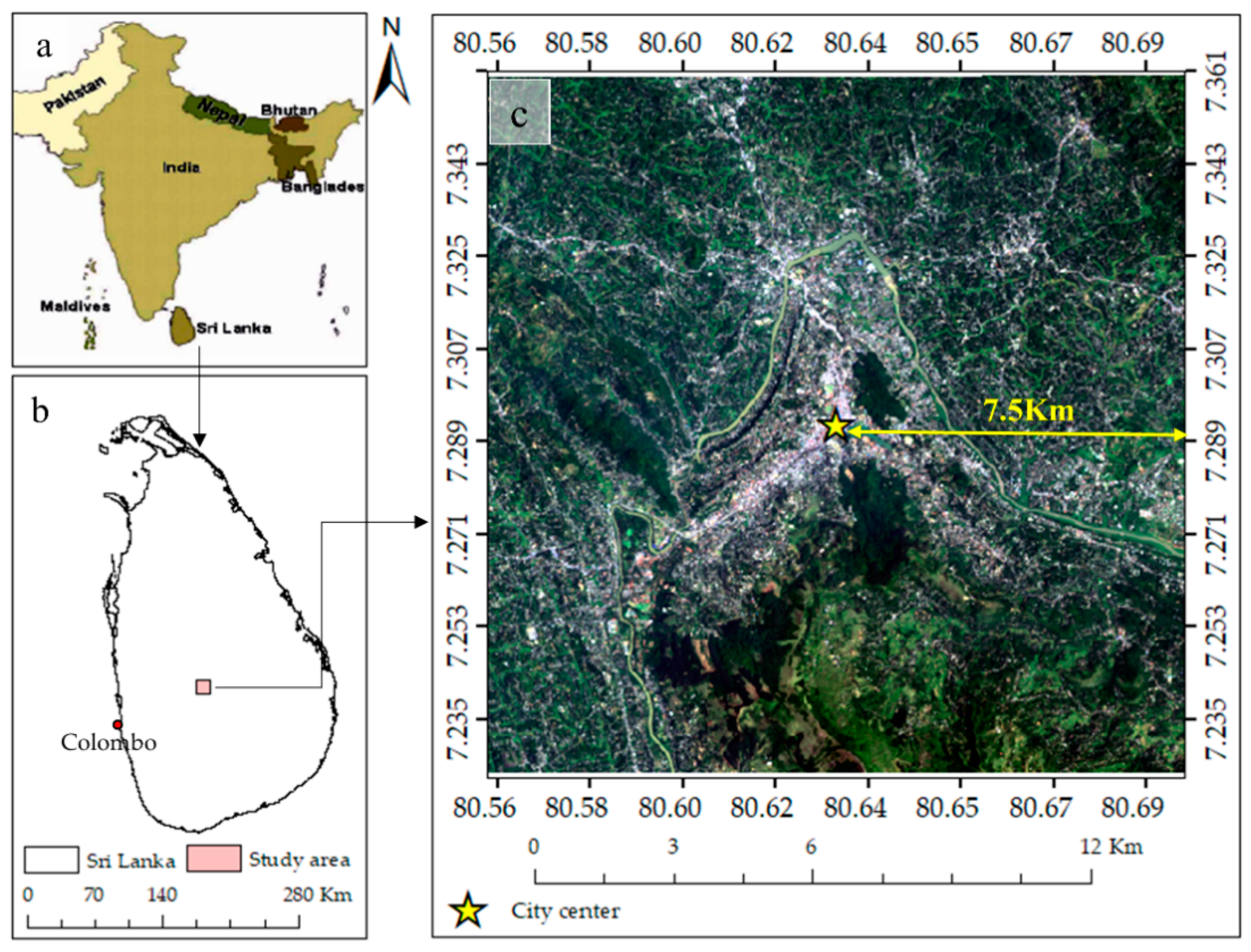
2.1. Study Area
2.2. Datasets and Data Preprocessing
2.3. LST Computation
2.4. Land-Use/Land-Cover (LULC) Classification
2.5. Adopted Method for Accuracy Assessment
2.6. Change Detection
2.7. Spatial Analysis
2.7.1. Urban Expansion and LST Behavior
2.7.2. Spatiotemporal Dynamic of IS as Grid-Based Density Analysis
3. Results
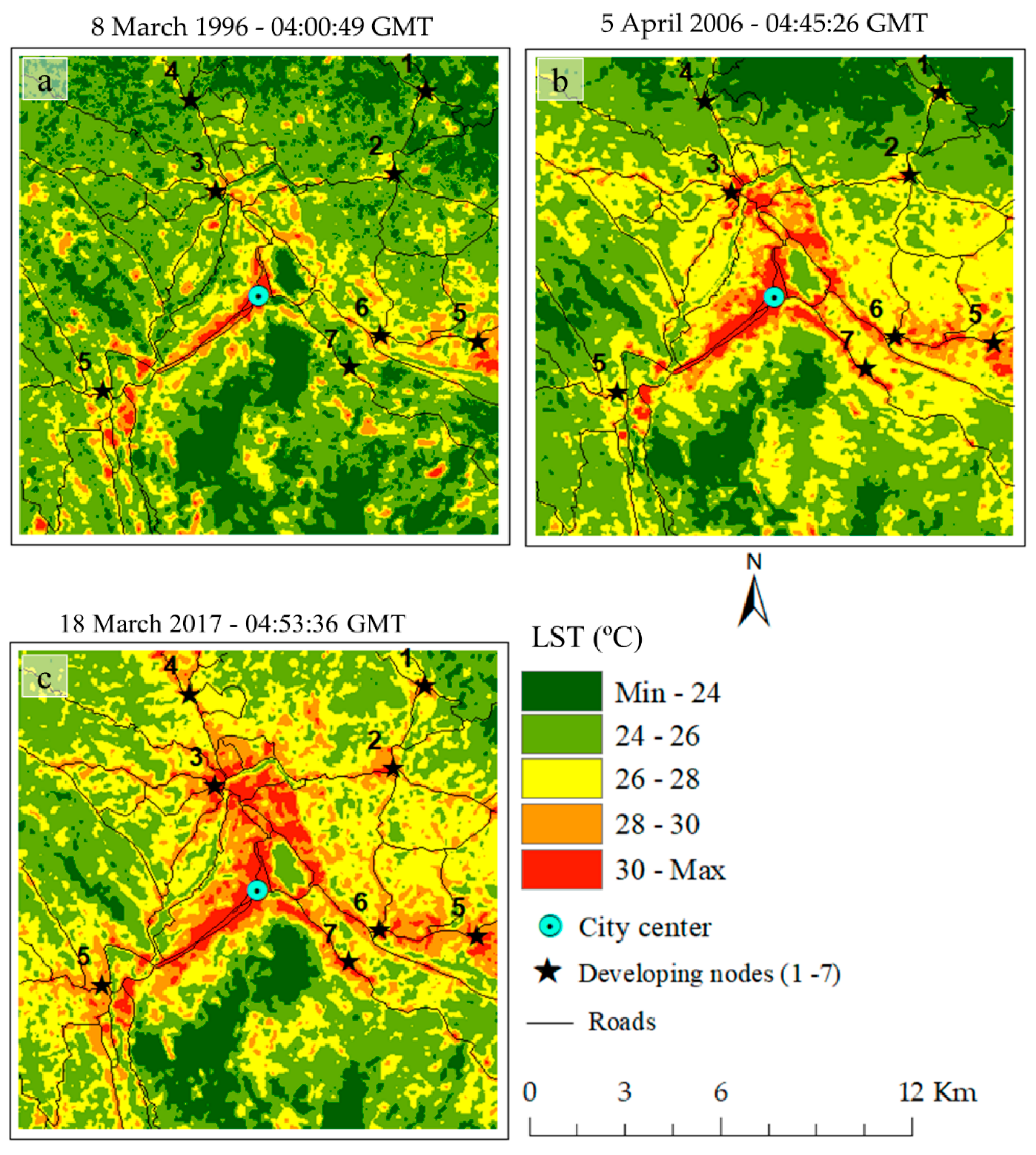
3.1. LST Spatiotemporal Pattern
3.2. Accuracy Assessment of LULC Classification
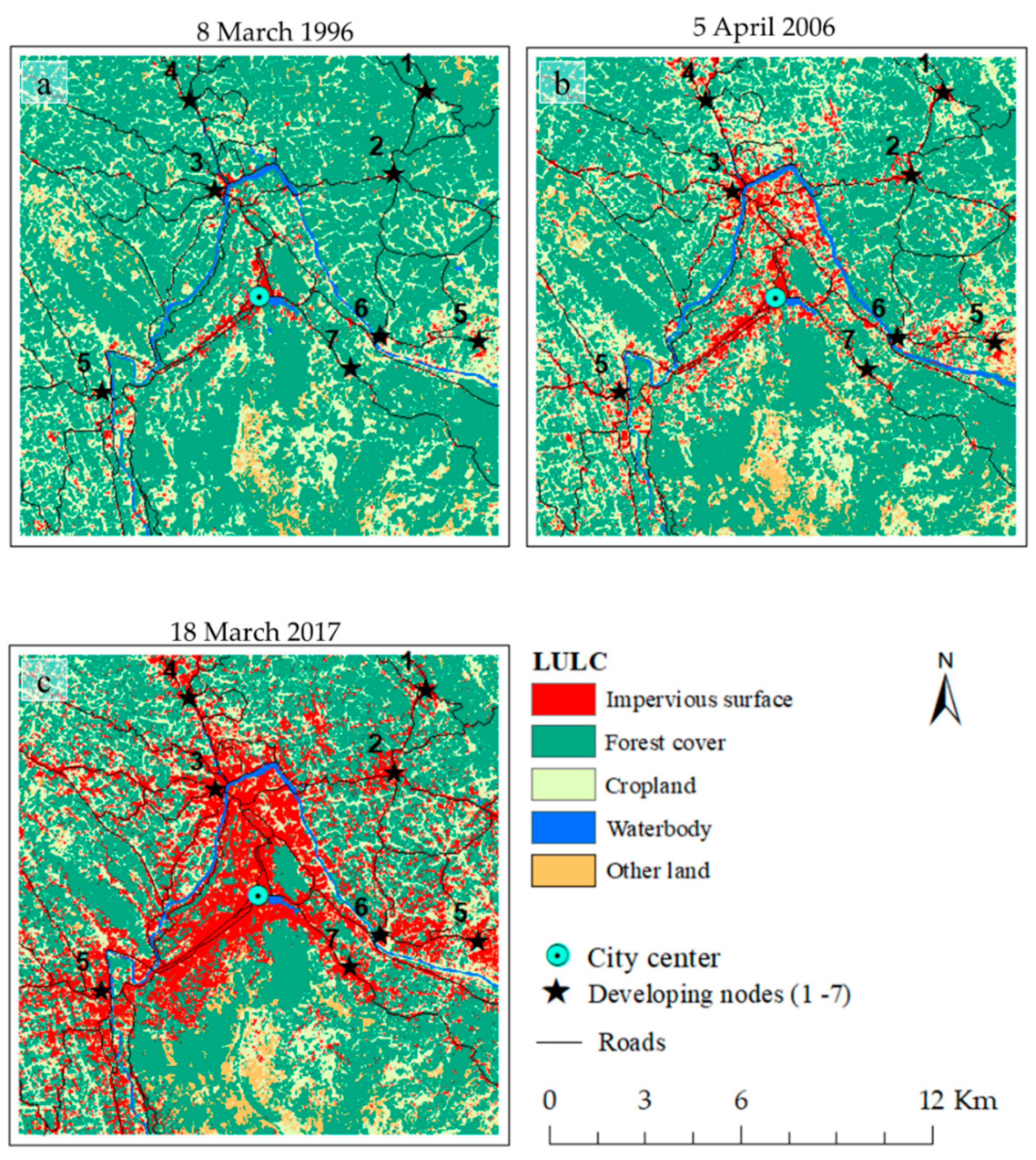
3.3. Spatiotemporal Pattern of LULC Dynamics
3.4. Urban Expansion and LST Behavior
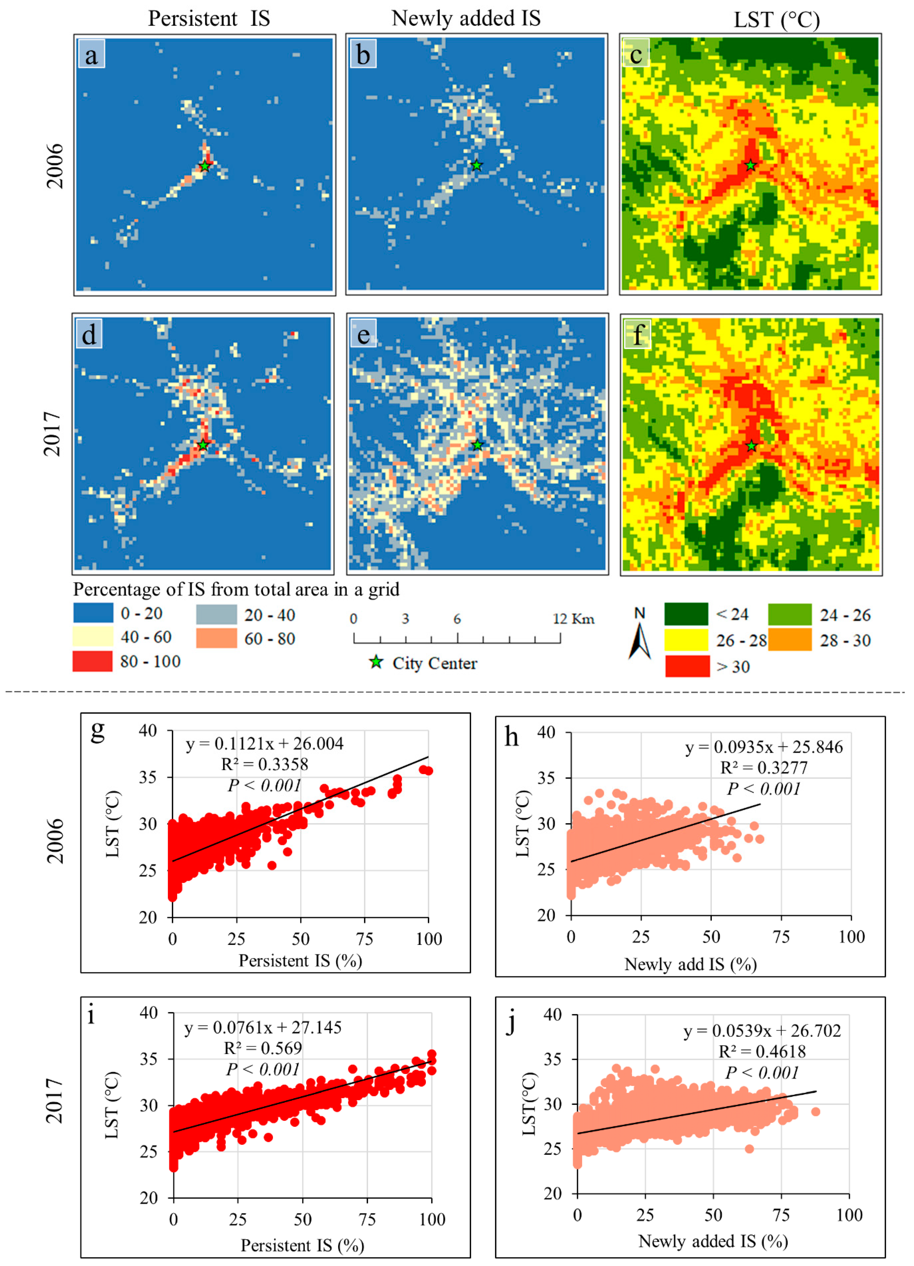
3.5. IS Spatiotemporal Dynamic
4. Discussion
4.1. Urbanization and SUHI Effect in Kandy City
4.2. Implication of Results for SUHI Mitigation and Adaptation
5. Conclusions
Author Contributions
Funding
Acknowledgments
Conflicts of Interest
References
- United Nations. UN Department of Economic and Social Affairs, The World ’s Cities in 2018; United Nations: New York, NY, USA, 2018. [Google Scholar]
- United Nations. UN Department of Economic and Social Affairs, World Urbanization Prospects: The 2014 Revision, Highlights; United Nations: New York, NY, USA, 2015. [Google Scholar]
- Dissanayake, D.; Morimoto, T.; Murayama, Y.; Ranagalage, M. Impact of landscape structure on the variation of land surface temperature in sub-saharan region: A case study of Addis Ababa using Landsat data (1986–2016). Sustainability 2019, 11, 2257. [Google Scholar] [CrossRef]
- Ranagalage, M.; Dissanayake, D.; Murayama, Y.; Zhang, X.; Estoque, R.C.; Perera, E.; Morimoto, T. Quantifying surface urban heat island formation in the world heritage tropical mountain city of Sri Lanka. ISPRS Int. J. Geo Inf. 2018, 7, 341. [Google Scholar] [CrossRef]
- Scafetta, N.; Ouyang, S. Detection of UHI bias in China climate network using Tmin and Tmax surface temperature divergence. Glob. Planet. Chang. 2019, 181, 102989. [Google Scholar] [CrossRef]
- Howard, L. The Climate of London; 1. W. Phillips: London, UK, 1818. [Google Scholar]
- EPA (US Environmental Protection Agency). Reducing Urban Heat Islands: Compendium of Strategies Urban Heat Island Basics; US Environmental Protection Agency: Washington, DC, USA, 2008.
- Oba, G. Urban heat island effect of Addis Ababa City: Implications of urban green spaces for climate change adaptation. In Climate Change Adaptation in Africa; Springer International Publishing: Berlin, Germany, 2017. [Google Scholar]
- Estoque, R.C.; Murayama, Y.; Myint, S.W. Effects of landscape composition and pattern on land surface temperature: An urban heat island study in the megacities of Southeast Asia. Sci. Total Environ. 2017, 577, 349–359. [Google Scholar] [CrossRef] [PubMed]
- Xu, S. An approach to analyzing the intensity of the daytime surface urban heat island effect at a local scale. Environ. Monit. Assess. 2009, 151, 289–300. [Google Scholar] [CrossRef]
- Li, Y.Y.; Zhang, H.; Kainz, W. Monitoring patterns of urban heat islands of the fast-growing Shanghai metropolis, China: Using time-series of Landsat TM/ETM+ data. Int. J. Appl. Earth Obs. Geoinf. 2012, 19, 127–138. [Google Scholar] [CrossRef]
- Senanayake, I.P.; Welivitiya, W.D.D.P.; Nadeeka, P.M. Remote sensing based analysis of urban heat islands with vegetation cover in Colombo city, Sri Lanka using Landsat-7 ETM+ data. Urban Clim. 2013, 5, 19–35. [Google Scholar] [CrossRef]
- Dissanayake, D.; Morimoto, T.; Murayama, Y.; Ranagalage, M.; Handayani, H.H. Impact of urban surface characteristics and socio-economic variables on the spatial variation of land surface temperature in Lagos City, Nigeria. Sustainability 2019, 11, 25. [Google Scholar] [CrossRef]
- Rousta, I.; Sarif, M.O.; Gupta, R.D.; Olafsson, H.; Ranagalage, M.; Murayama, Y.; Zhang, H.; Mushore, T.D. Spatiotemporal analysis of land use/land cover and its effects on Ssurface urban heat island using landsat data: A case study of metropolitan city Tehran (1988–2018). Sustainability 2018, 10, 4433. [Google Scholar] [CrossRef]
- Myint, S.W.; Brazel, A.; Okin, G.; Buyantuyev, A. Combined effects of impervious surface and vegetation cover on air temperature variations in a rapidly expanding desert city. GISci. Remote Sens. 2010, 47, 301–320. [Google Scholar] [CrossRef]
- Estoque, R.C.; Murayama, Y. Monitoring surface urban heat island formation in a tropical mountain city using Landsat data (1987–2015). ISPRS J. Photogramm. Remote Sens. 2017, 133, 18–29. [Google Scholar] [CrossRef]
- Ranagalage, M.; Estoque, R.C.; Murayama, Y. An urban heat island study of the Colombo metropolitan area, Sri Lanka, based on Landsat data (1997–2017). ISPRS Int. J. Geo-Inf. 2017, 6, 189. [Google Scholar] [CrossRef]
- Ranagalage, M.; Estoque, R.C.; Zhang, X.; Murayama, Y. Spatial changes of urban heat island formation in the Colombo District, Sri Lanka: Implications for sustainability planning. Sustainability 2018, 10, 1367. [Google Scholar] [CrossRef]
- Kikon, N.; Singh, P.; Singh, S.K.; Vyas, A. Assessment of urban heat islands (UHI) of Noida City, India using multi-temporal satellite data. Sustain. Cities Soc. 2016, 22, 19–28. [Google Scholar] [CrossRef]
- Arsiso, B.K.; Mengistu Tsidu, G.; Stoffberg, G.H.; Tadesse, T. Influence of urbanization-driven land use/cover change on climate: The case of Addis Ababa, Ethiopia. Phys. Chem. Earth 2018, 105, 212–223. [Google Scholar] [CrossRef]
- Oke, T.R. City size and the urban heat island. Atmos. Environ. 1973, 7, 769–779. [Google Scholar] [CrossRef]
- Ranagalage, M.; Wang, R.; Gunarathna, M.H.J.P.; Dissanayake, D.; Murayama, Y.; Simwanda, M. Spatial forecasting of the landscape in rapidly urbanizing hill stations of South Asia: A case study of Nuwara Eliya, Sri Lanka (1996–2037). Remote Sens. 2019, 11, 1743. [Google Scholar] [CrossRef]
- Simwanda, M.; Ranagalage, M.; Estoque, R.C.; Murayama, Y. Spatial analysis of surface urban heat islands in four rapidly growing African Cities. Remote Sens. 2019, 11, 1645. [Google Scholar] [CrossRef]
- Dissanayake, D.; Morimoto, T.; Ranagalage, M. Accessing the soil erosion rate based on RUSLE model for sustainable land use management: A case study of the Kotmale watershed, Sri Lanka. Model. Earth Syst. Environ. 2018, 5, 291–306. [Google Scholar] [CrossRef]
- Wijesundara, N.C.; Abeysingha, N.S.; Dissanayake, D.M.S.L.B. GIS-based soil loss estimation using RUSLE model: A case of Kirindi Oya river basin, Sri Lanka. Model. Earth Syst. Environ. 2018, 4, 251–262. [Google Scholar] [CrossRef]
- Dienst, M.; Lindén, J.; Saladié, Ò.; Esper, J. Detection and elimination of UHI effects in long temperature records from villages—A case study from Tivissa, Spain. Urban Clim. 2019, 27, 372–383. [Google Scholar] [CrossRef]
- Daskon, C.D. Cultural resilience–The roles of cultural traditions in sustaining rural livelihoods: A case study from rural Kandyan villages in central Sri Lanka. Sustainability 2010, 2, 1080–1100. [Google Scholar] [CrossRef]
- Weerasundara, L.; Magana-Arachchi, D.N.; Ziyath, A.M.; Goonetilleke, A.; Vithanage, M. Health risk assessment of heavy metals in atmospheric deposition in a congested city environment in a developing country: Kandy City, Sri Lanka. J. Environ. Manag. 2018, 220, 198–206. [Google Scholar] [CrossRef] [PubMed]
- Ministry of Urban Development, Water Supply and Drainage Sri Lanka. Kandy City Region Strategic Development Plan—2030; Urban Development Authority: Kandy, Sri Lanka, 2015.
- Meetiyagoda, L. Pedestrian safety in Kandy Heritage City, Sri Lanka: Lessons from world heritage cities. Sustain. Cities Soc. 2018, 38, 301–308. [Google Scholar] [CrossRef]
- United States Geological Survey (USGS). Landsat Missions: Landsat Science Products. Available online: https://www.usgs.gov/land-resources/nli/landsat/landsat-science-products (accessed on 7 April 2018).
- Sobrino, J.A.; Jiménez-Muñoz, J.C.; Paolini, L. Land surface temperature retrieval from Landsat TM 5. Remote Sens. Environ. 2004, 90, 434–440. [Google Scholar] [CrossRef]
- Weng, Q.; Lu, D.; Schubring, J. Estimation of land surface temperature-vegetation abundance relationship for urban heat island studies. Remote Sens. Environ. 2004, 89, 467–483. [Google Scholar] [CrossRef]
- Ibrahim, M.; Abu-Mallouh, H. Estimate land surface temperature in relation to land use types and geological formations using spectral remote sensing data in Northeast Jordan. Open J. Geol. 2018, 8, 174–185. [Google Scholar] [CrossRef][Green Version]
- Weng, Q. Land use change analysis in the Zhujiang Delta of China using satellite remote sensing, GIS and stochastic modelling. J. Environ. Manag. 2002, 64, 273–284. [Google Scholar] [CrossRef]
- Phiri, D.; Morgenroth, J. Developments in Landsat land cover classification methods: A review. Remote Sens. 2017, 9, 967. [Google Scholar] [CrossRef]
- Erkan, U.; Gökrem, L. A new method based on pixel density in salt and pepper noise removal. Turk. J. Electr. Eng. Comput. Sci. 2018, 26, 162–171. [Google Scholar] [CrossRef]
- Thapa, R.; Murayama, Y. Image classification techniques in mapping urban landscape: A case study of Tsukuba city using AVNIR-2 sensor data. Tsukuba Geoenviron Ment. Sci. 2007, 3, 3–10. [Google Scholar]
- Sakthidasan Sankaran, K.; Velmurugan Nagappan, N. Noise free image restoration using hybrid filter with adaptive genetic algorithm. Comput. Electr. Eng. 2016, 54, 382–392. [Google Scholar] [CrossRef]
- Wu, C.; Murray, A.T. Estimating impervious surface distribution by spectral mixture analysis. Remote Sens. Environ. 2003, 84, 493–505. [Google Scholar] [CrossRef]
- Weng, Q. A remote sensing–GIS evaluation of urban expansion and its impact on surface temperature in the Zhujiang Delta, China. Int. J. Remote Sens. 2001, 22, 1999–2014. [Google Scholar]
- Pal, S.; Ziaul, S. Detection of land use and land cover change and land surface temperature in English Bazar urban centre. Egypt. J. Remote Sens. Sp. Sci. 2017, 20, 125–145. [Google Scholar] [CrossRef]
- Ahmed Memon, R.; Leung, D.Y.; Chunho, L. A review on the generation, determination and mitigation of Urban Heat Island. J. Environ. Sci. 2008, 20, 120–128. [Google Scholar]
- Lea, C.; Curtis, A.C. Thematic Accuracy Assessment Procedures, Natural Resource Report NPS/NRPC/NRR—2010/204 NPS 999/10; U.S. Department of the Interior, National Park Service, Natural Resource Program Center: Fort Collins, CO, USA, 2010.
- Galagoda, R.U.; Jayasinghe, G.Y.; Halwatura, R.U.; Rupasinghe, H.T. The impact of urban green infrastructure as a sustainable approach towards tropical micro-climatic changes and human thermal comfort. Urban For. Urban Green. 2018, 34, 1–9. [Google Scholar] [CrossRef]
- Ranagalage, M.; Estoque, R.C.; Handayani, H.H.; Zhang, X.; Morimoto, T.; Tadono, T.; Murayma, Y. Relation between urban volume and land surface temperature: A comparative study of planned and traditional cities in Japan. Sustainability 2018, 10, 2366. [Google Scholar] [CrossRef]
- Min, C.M.; Min, H.Z. Spatio-temporal evolution analysis of the urban heat island: A case study of Zhengzhou City, China. Sustainability 2018, 10, 1992. [Google Scholar] [CrossRef]
- Lin, J.; Huang, B.; Chen, M.; Huang, Z. Modeling urban vertical growth using cellular automata–Guangzhou as a case study. Appl. Geogr. 2014, 53, 172–186. [Google Scholar] [CrossRef]
- Handayani, H.H.; Murayama, Y.; Ranagalage, M.; Liu, F.; Dissanayake, D. Geospatial analysis of horizontal and vertical urban expansion using multi-spatial resolution data: A case study of Surabaya, Indonesia. Remote Sens. 2018, 10, 1599. [Google Scholar] [CrossRef]
- Weerasundara, L.; Amarasekara, R.W.K.; Magana-Arachchi, D.N.; Ziyath, A.M.; Karunaratne, D.G.G.P.; Goonetilleke, A.; Vithanage, M. Microorganisms and heavy metals associated with atmospheric deposition in a congested urban environment of a developing country: Sri Lanka. Sci. Total Environ. 2017, 584–585, 803–812. [Google Scholar] [CrossRef] [PubMed]
- Aberatne, V.D.; Illeperuma, O. Air pollution monitoring in the city of Kandy: Possible transboundary effects. Natl. Sci. Found. Sri Lanka 2006, 34, 137–141. [Google Scholar] [CrossRef]
- Zhang, X.; Estoque, R.C.; Murayama, Y. An urban heat island study in Nanchang City, China based on land surface temperature and social-ecological variables. Sustain. Cities Soc. 2017, 32, 557–568. [Google Scholar] [CrossRef]


| (a) Metadata of Landsat images | |||
| Sensor | Landsat-5 TM | Landsat-5 TM | Landsat-8 OLI/TIRS |
| Landsat Sensor ID | LT05_L1TP_141055_19960308_20170106_01_T1 | LT05_L1TP_141055_20060405_20161123_01_T | LC08_L1TP_141055_20170318_20170328_01_T1 |
| Date | 8 March 1996 | 5 April 2006 | 18 March 2017 |
| Spatial Resolution | 30 × 30 m | ||
| Path/Row | 141/55 | ||
| Time (GMT)* | 4:00:49 a.m. | 4:45:26 a.m. | 4:53:36 a.m. |
| (b) Air temperature (°C) of image acquisition dates. (Data source: Department of Meteorology, Sri Lanka) | |||
| Maximum | 32 | 31.5 | 30.8 |
| Minimum | 19.4 | 20.4 | 16.1 |
| Mean | 25.7 | 25.9 | 23.4 |
| Calculation/Process | Mathematical Equation | Description | Equation. No. |
|---|---|---|---|
| Normalized Difference Vegetation Index | ρNIR refers to surface-reflectance values of Band 4 (Landsat-5 TM) and Band 5 (Landsat-8); ρRed refers to the surface-reflectance values of Band 3 (Landsat-5 TM) and Band 4 (Landsat-8 OLI). | (1) | |
| Proportion of Vegetation (Pv) | Pv represents the amount of vegetation, NDVImin represents minimum values of normalized difference vegetation index (NDVI), and NDVImax represents the maximum value of NDVI. | (2) | |
| Land-Surface Emissivity (ε) | ε represents land-surface emissivity; m represents (εv − εs) − (1 − εs) Fεv; Pv represents the amount of vegetation; n represents εs + (1 − εs) Fεv; εs is soil emissivity; εv is vegetation emissivity; and F is a shape factor whose mean value, assuming different geometrical distributions, is 0.55 [32]. In this study, we adopted m as 0.004 and n as 0.986 based on previous results [32]. | (3) | |
| Emissivity-Corrected LST | Tb is at-satellite brightness temperature in Kelvin; λ is central-band wavelength of emitted radiance (11.5 μm for Band 6 and 10.8 μm for Band 10 [33]); is h × c/σ (1.438 × 10⁻² m K) with σ being the Boltzmann constant (1.38 × 10⁻²³ J/K), h is Planck’s constant (6.626 × 10⁻³⁴ J∙s), and c is the speed of light (2.998 × 10⁸ m/s) [34]; ε is land-surface emissivity estimated using Equation (3). Then, calculated LST values (Kelvin) were converted to degrees Celsius (°C). | (4) |
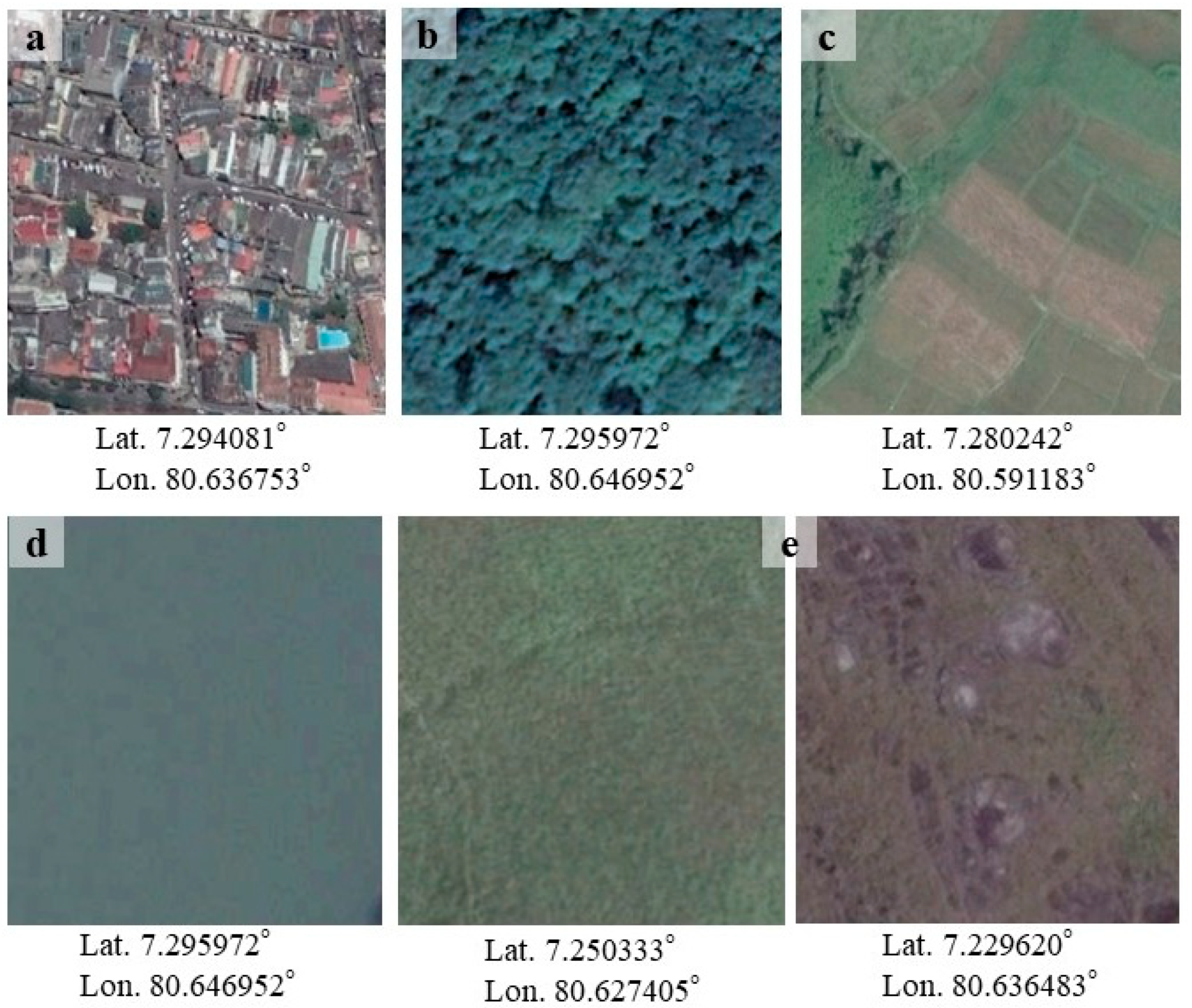
| LULC | Code | Description | Image Reference * |
|---|---|---|---|
| Impervious surface | IS | Areas with a very high urban proportion, including the central business district, and commercial, industrial, and residential lands. | a |
| Forest cover | FC | Areas with a high vegetation fraction, including dense and less dense forests with evergreen trees. | b |
| Croplands | CL | Agricultural lands, including paddy, tea, and other farmlands. | c |
| Waterbody | WB | Areas covered by water, including rivers, tanks, and ponds. | d |
| Other land | OL | Other LULC not included in the above categories. | e |
| LULC | 1996 | 2006 | 2017 | |
|---|---|---|---|---|
| User accuracy (%) | IS | 83.3 | 97.1 | 99.2 |
| FC | 95.2 | 99.3 | 98.7 | |
| CL | 94.2 | 90.2 | 92.4 | |
| WB | 100 | 100 | 80 | |
| OL | 92 | 90.3 | 86.4 | |
| Producer accuracy (%) | IS | 100 | 97.1 | 99.2 |
| FC | 98.8 | 95.9 | 95.4 | |
| CL | 89.8 | 97.7 | 96.5 | |
| WB | 100 | 100 | 100 | |
| OL | 69.7 | 87.5 | 90.5 | |
| Overall accuracy (%) | 94.6 | 96 | 96.4 | |
| Kappa coefficient | 0.89 | 0.93 | 0.95 |
| LULC | 1996 | 2006 | 2017 | |||
|---|---|---|---|---|---|---|
| Area (ha) | Percentage (%) | Area (ha) | Percentage (%) | Area (ha) | Percentage (%) | |
| IS | 528.7 | 2.3 | 1514.0 | 6.7 | 5382.5 | 23.9 |
| FC | 15,041.9 | 66.9 | 12,742.1 | 56.6 | 10,483.4 | 46.6 |
| CL | 5570.8 | 24.8 | 6486.3 | 28.8 | 5372.6 | 23.9 |
| WB | 248.2 | 1.1 | 296.5 | 1.3 | 239.6 | 1.1 |
| OL | 1110.4 | 4.9 | 1461.2 | 6.5 | 1022.0 | 4.5 |
| Total | 22,500.0 | 100.0 | 22,500.0 | 100.0 | 22,500.0 | 100.0 |
| LULC | 1996 vs. 2006 | 2006 vs. 2017 | 1996 vs. 2017 | ||||||
|---|---|---|---|---|---|---|---|---|---|
| Net change | Annual change | Annual change rate (%) | Net change | Annual change | Annual change rate (%) | Net change | Annual change | Annual change rate | |
| (ha) | (ha) | (ha) | (ha) | (ha) | (ha) | (%) | |||
| IS | 985.3 | 98.5 | 11.1 | 3868.5 | 351.7 | 12.2 | 4853.8 | 231.1 | 11.7 |
| FC | −2299.8 | −230 | −1.6 | −2258.7 | −205.3 | −1.8 | −4558.5 | −217.1 | −1.7 |
| CL | 915.5 | 91.5 | 1.5 | −1113.7 | −101.2 | −1.7 | −198.2 | −9.4 | −0.2 |
| WB | 48.2 | 4.8 | 1.8 | −56.9 | −5.2 | 11.9 | −8.6 | −0.4 | −0.2 |
| OL | 350.7 | 35.1 | 2.8 | −439.2 | −39.9 | −3.2 | −88.5 | −4.2 | −0.4 |
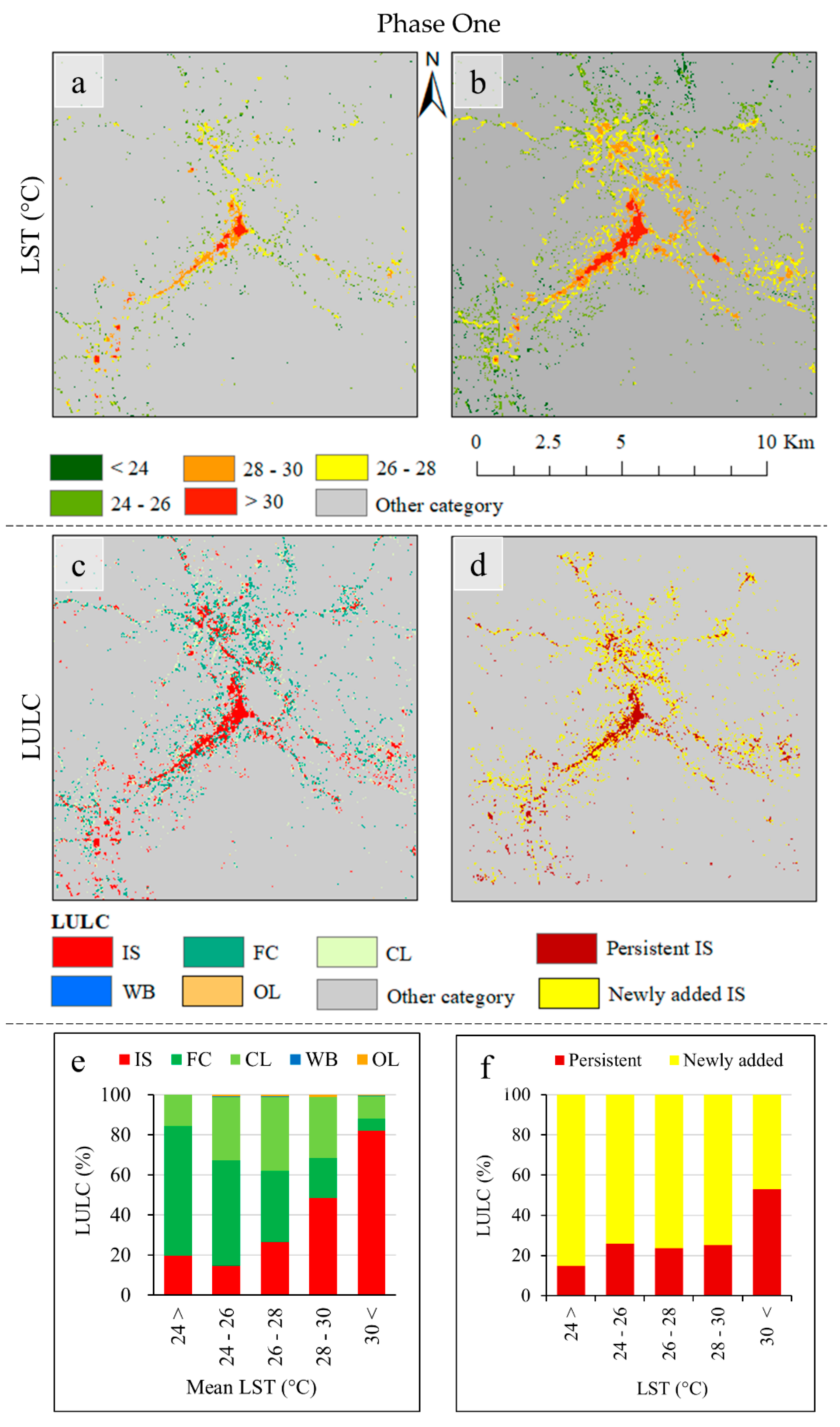
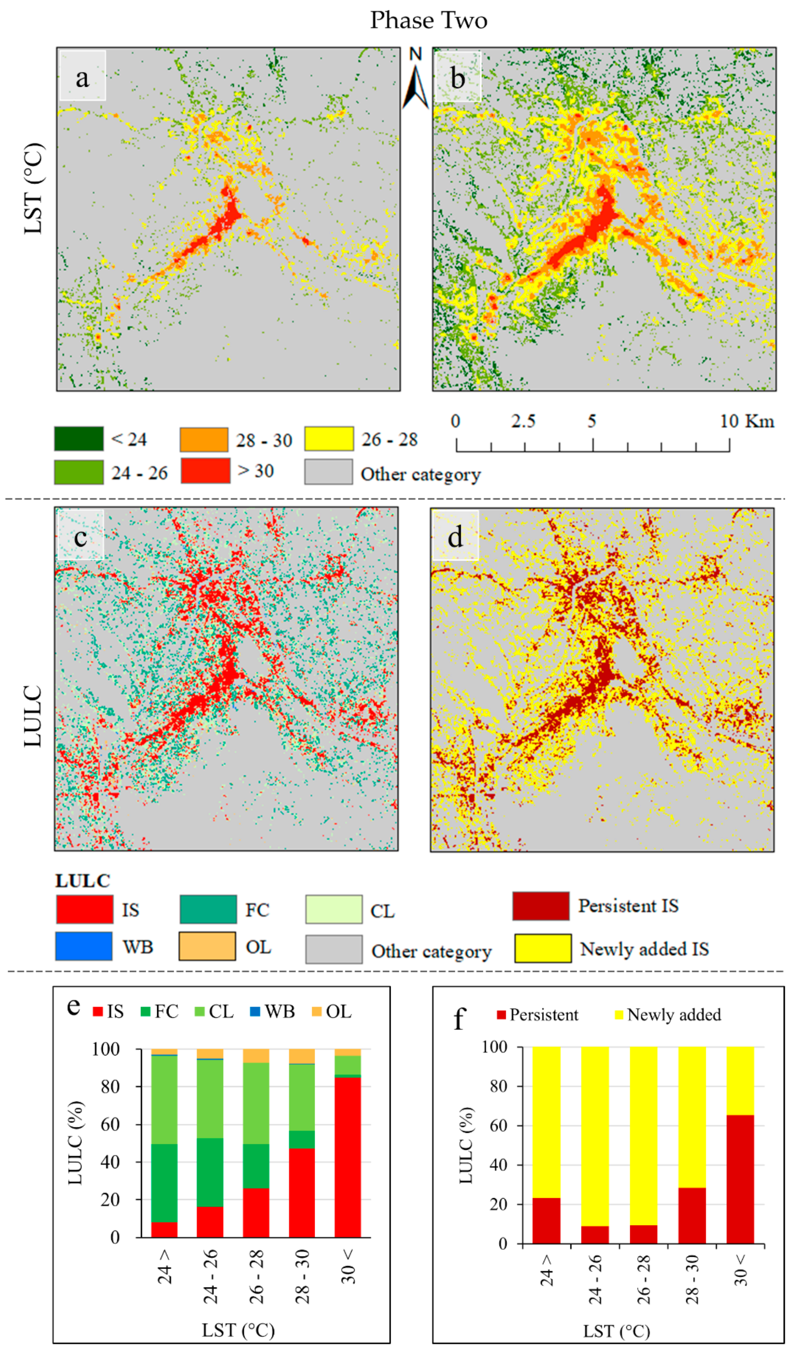
| Attributes | Phase One | Phase Two |
|---|---|---|
| Period | 1996–2006 | 2006–2017 |
| LULC | The LULC that transferred to IS from 1996 to 2006 (newly added IS) and persistent IS in 2006 as a percentage from total land by following LST classes. | Other LULC that transferred to IS from 2006 to 2017 (newly added IS) and persistent IS in 2017 as a percentage from total land by following LST classes. |
| LST | LST spatial pattern over the above LULC in 1996 and 2006 | LST spatial pattern over the above LULC in 2006 and 2017 |
| LST classes | <24, 24–26, 26–28, 28–30, >30 | |
| Respective figure caption | Figure 5a–f | Figure 6a–f |
| (a) Area of total IS, persistent IS, and newly added IS (ha) | |||
| Phase One (2006) | Phase Two (2017) | Change (2017–2006) | |
| Total IS | 1514.0 | 5382.5 | 3868.5 |
| Persistent IS | 524.3 | 1503.6 | 979.3 |
| Newly added IS | 989.6 | 3878.8 | 2889.2 |
| (b) Mean LST by types of IS (°C) | |||
| Phase One (2006) | Phase Two (2017) | Change (2017–2006) | |
| Total IS | 28.79 | 29.24 | 0.45 |
| Persistent IS | 29.63 | 30.39 | 0.77 |
| Newly added IS | 28.35 | 28.80 | 0.44 |
| (c) Differences in LST between the types of IS (°C) | |||
| Cross-cover comparison | Phase One (2006) | Phase Two (2017) | Mean (2017–2006) |
| Total IS–persistent IS | −0.83 | −1.15 | −0.99 |
| Total IS–newly added IS | 0.44 | 0.45 | 0.44 |
| Persistent IS–newly added IS | 1.27 | 1.59 | 1.43 |
© 2019 by the authors. Licensee MDPI, Basel, Switzerland. This article is an open access article distributed under the terms and conditions of the Creative Commons Attribution (CC BY) license (http://creativecommons.org/licenses/by/4.0/).
Share and Cite
Dissanayake, D.; Morimoto, T.; Ranagalage, M.; Murayama, Y. Land-Use/Land-Cover Changes and Their Impact on Surface Urban Heat Islands: Case Study of Kandy City, Sri Lanka. Climate 2019, 7, 99. https://doi.org/10.3390/cli7080099
Dissanayake D, Morimoto T, Ranagalage M, Murayama Y. Land-Use/Land-Cover Changes and Their Impact on Surface Urban Heat Islands: Case Study of Kandy City, Sri Lanka. Climate. 2019; 7(8):99. https://doi.org/10.3390/cli7080099
Chicago/Turabian StyleDissanayake, DMSLB, Takehiro Morimoto, Manjula Ranagalage, and Yuji Murayama. 2019. "Land-Use/Land-Cover Changes and Their Impact on Surface Urban Heat Islands: Case Study of Kandy City, Sri Lanka" Climate 7, no. 8: 99. https://doi.org/10.3390/cli7080099
APA StyleDissanayake, D., Morimoto, T., Ranagalage, M., & Murayama, Y. (2019). Land-Use/Land-Cover Changes and Their Impact on Surface Urban Heat Islands: Case Study of Kandy City, Sri Lanka. Climate, 7(8), 99. https://doi.org/10.3390/cli7080099