Atmospheric and Ocean Dynamics May Explain Cycles in Oceanic Oscillations

Abstract

What causes cycles in oceanic oscillations, and is there a change in the characteristics of oscillations in around 1950? Characteristics of oceanic cycles and their sources are important for climate predictability. We here compare cycles generated in a simple model with observed oceanic cycles in the great oceans: The North Atlantic Oscillation (NAO), El Niño, the Southern Oscillation Index (SOI), and the Pacific Decadal Oscillation (PDO). In the model, we let a stochastic movement in one oceanic oscillation cause a similar but lagging movement in another oceanic oscillation. The two interacting oscillations show distinct cycle lengths depending upon how strongly one oscillation creates lagging cycles in the other. The model and observations both show cycles around two to six, 13 to 16, 22 to 23, and 31 to 32 years. The ultimate cause for the distinct cycles is atmospheric and oceanic “bridges” that connect the ocean basins, but the distinct pattern in cycle lengths is determined by properties of statistical distributions. We found no differences in the leading or lagging strength between well separated basins (the North Atlantic and the Pacific) and overlapping ocean basins (both in the Pacific). The cyclic pattern before 1950 appears to be different from the cyclic pattern after 1950.

1. Introduction

Several attempts have been made to explain the cycles observed for El Niño as well as for other ocean oscillations [1,2,3], and the observational procedures for obtaining data that characterize El Niño have been improved, in particular after about 1950 [4]. The El Niño and other measures of the Pacific oscillations are often quoted to show oscillations from two to seven years, [2,5], but multidecadal and longer cycles have also been identified [6,7]

There are several assessments of the cyclic nature of the various ocean oscillations that are invoked in explaining global and local temperature changes [8,9,10]. Four recent explanations for the observed ocean oscillation are: (i) One refers to the movements of the sun and the moon, but requires amplifying mechanisms to drive the oscillations (e.g., Keeling and Whorf [11], Munk et. al [12], Treolar [13]). (ii) A second recent explanation suggests that the net top-of-the-atmosphere (TOA) energy flux explains part of the mean ocean heating rate (correlation coefficient 0.53) [14,15]. However, changes in the TOA energy flux may be associated with variations in atmospheric greenhouse gases, CO₂ → TOA flux → ocean heat uptake. (iii) A third explanation relates to ocean morphology and “memory,” stochastic forces, and mechanisms that cause out-of-phase oscillations in the Pacific [16]. (iv) A fourth explanation is that the cyclic characteristics of the Pacific Decadal Oscillation (PDO) and the Southern Oscillation Index (SOI) could be explained by the strength of the interaction between ocean oscillations, Seip and Grøn [17]. The oscillations initially show stochastic movements, but subsequently one of the oscillations influence a neighboring oscillation so that the movements in both oscillations become synchronized, but with a lag for one of them. The two series are then said to show a leading–lagging (LL) relationship. The two-oscillation systems then show characteristic common cycle times. However, the El Niño–Southern Oscillation (ENSO) shows “ENSO flavors,” that is, the sea surface temperature (SST) of different ENSO events varies in amplitude and frequency, suggesting that there may be other factors involved as well [2,18].

The objective of the present study is to obtain a better understanding of the characteristics of ocean oscillations. For example, Delworth et al. (2017) suggest that ocean dynamics are critical to the interaction between the North Atlantic Oscillation (NAO) and the Atlantic Multidecadal Oscillation (AMO), but that the NAO and the Atlantic Meridional Overturning Circulation (AMOC) also involve atmospheric processes, like cloud or dust feedbacks.

Detailed mechanisms can be found in articles that include model descriptions (e.g., Jackson et al. [19] on salinity and the AMOC). Williamson et al. [5] discuss the relationship between temperature dipoles and wind stress, Vannitsem and Ekelmans [20] discuss thermohaline circulation, and Busecke and Abernathey [21] discuss ocean mesoscale mixing driven by variations in large-scale flow.

Here we show that ocean oscillation interactions impact oscillation periodicity, and that the mechanisms that explain the strength of ocean interactions may be sufficient to predict the periodicities. We expand on the model for ocean oscillation cycle lengths by Seip and Grøn [17]. In particular, we examine further the impact of the persistent leading or lagging relations between oceanic oscillations. Since observation procedures for El Niño were improved around 1950, we examine if data on ocean oscillations before 1950 differ from data after 1950. A similar improvement in data quality occurred for the Northern Hemisphere sea level pressure and the North Atlantic sea ice cover in 1950 [6]. There is also a concern that the effects of progressively increasing atmospheric CO₂ concentrations may change the way ocean oscillations interact [22]. Lastly, we examine the actual persistence of LL relations between NAO and El Niño (different ocean basins) and PDO and El Niño (overlapping ocean basins).

2. Materials

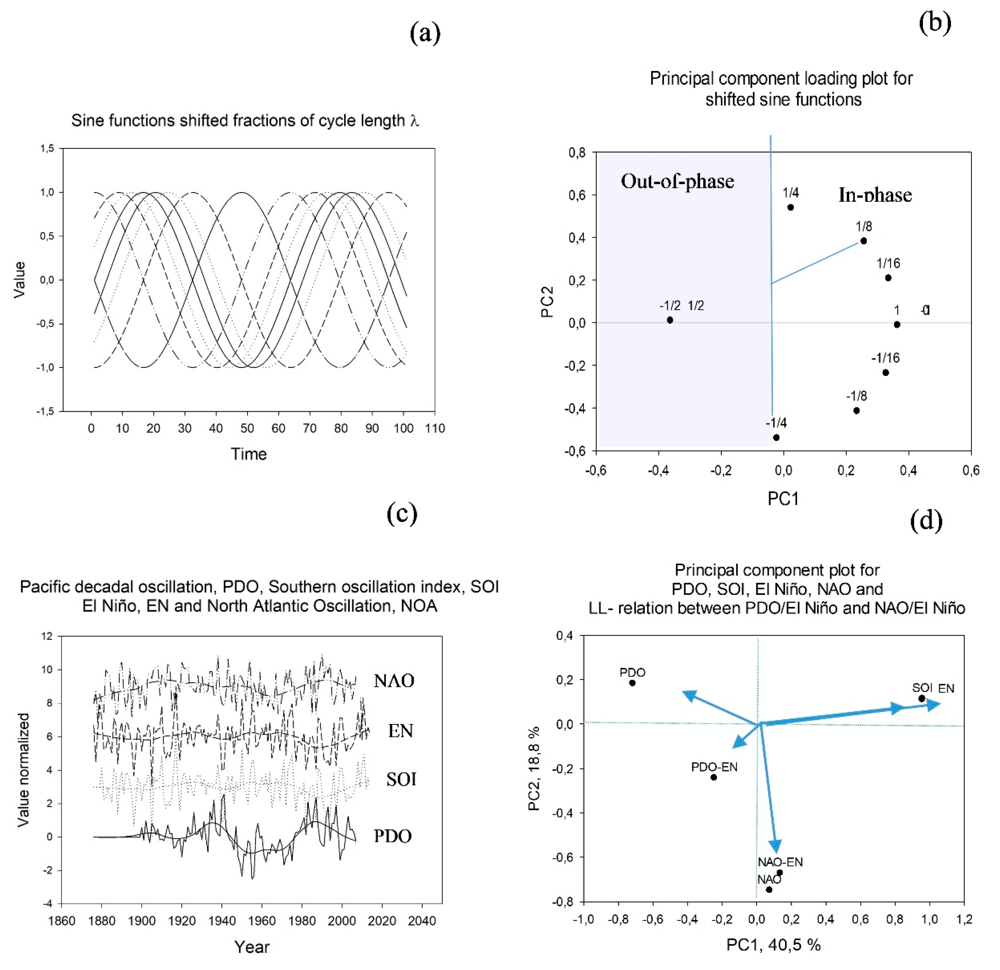
We tested four ocean oscillations, or proxies for the oscillations, that were closely related to the climate variability and global warming. They were the Pacific Decadal Oscillation (PDO), the Southern Oscillation Index (SOI), the El Niño, and the North Atlantic Oscillation (NAO), Figure 1c. The PDO and the El Niño were measures of SST, the others of pressure differences. The pressure difference series were assumed to express characteristics of ocean oscillations within an ocean region, but require physical mechanisms to link them to oscillations in SST. The regions may differ, as for the El Niño that are specified by region numbers 1, 2, 3, and 4 in the Pacific [23].

For the raw series examined here, Privalsky and Yushkov [24] characterize the series in terms of the order, p, corresponding to a discrete autoregressive time series (AR(p)) and (r_e) that characterize the series proximity to white noise. The numbers identified by Privalsky and Yushkov [24] are quoted below.

The Pacific Decadal Oscillation (PDO) is closely related to the Interdecadal Pacific Oscillation (IPO), but has a more northern hemisphere focus (Gehne et al. 2014; Trenberth 2015). PDO was measured by the PDO index. Cycle length for PDO after isolating multidecadal variability was about 50–70 years [25,26]. We used annual data from 1861 to 2015 for this series. The Privalsky and Yushkov [24] characteristics were AR(p) = 1 and re = 0.10, that is, 90% of the variations in the time series were due to noise. Data were retrieved from http://www.atmos.washington.edu/~mantua/abst.PDO.html).

The Southern Oscillation Index (SOI) is a standardized index based on the observed sea level pressure differences between Tahiti and Darwin, Australia (P_Tahiti − P_Darwin). The negative phase of the SOI represents below-normal air pressure at Tahiti and above-normal air pressure at Darwin. Prolonged periods of negative (positive) SOI values coincide with abnormally warm (cold) ocean waters across the eastern tropical Pacific typical of El Niño (La Niña) episodes.

The Privalsky and Yushkov [24] characteristics were AR(p) = 2 and r_e = 0.08. Data were retrieved from http://www.bom.gov.au/climate/current/soihtm1.shtml.

The Niño 3.4 index was the average of SSTA in the Niño 3.4 region (120°W–170°W, 5°S–5°N), with the unit of K (or °C). The index was used to represent the variability of the El Niño–Southern Oscillation (ENSOs). An increase in the El Niño index above say +0.5 indicates that the east–central tropical Pacific is warmer than normal. The El Niño–Southern Oscillation (ENSO) was reported to show periodicities of two to seven years [27] and to interact with the PDO or the Interdecadal Pacific Oscillation (IPO), which is closely related to PDO [28]. The Privalsky and Yushkov [24] characteristics were NINO4a: AR(p) = 2 and re = 0.13. Data were retrieved from https://www.ncdc.noaa.gov/teleconnections/enso/indicators/soi/.

The North Atlantic Oscillation (NAO) measures the air pressure difference between a Southern station (e.g., Lisbon and the Northern station, Reykjavik (p _Lisbon − p _Reykjavik)). When the NAO index exhibits an increasing trend, European winter-time temperatures are frequently higher than normal. [29,30]. The cycle length for the NAO when smoothed to identify multidecadal variability is about 60 years [31,32]. On an interannual time scale, the dynamics of the North Pacific and the North Atlantic probably influence each other through thermocline circulation [20]. The Privalsky and Yushkov [24] characteristics were AR(p) = 0 and r_e = 0. Although these authors found that the NAO is purely stochastic, the NAO time series are used to explain, for example, ocean circulation (Woollings et al. [33]) and Northern winter temperatures (Faust et al. [34]). Seip et al. [35] show that the NAO has common cycle times with other North Atlantic Oscillation measures, like the AMO and the AMOC. We used annual NAO index values obtained from the website: https://climatedataguide.ucar.edu/climate-data/hurrell-north-atlantic-oscillation-nao-index-station-based.

The time series start at different years ranging from 1861–1900. For the calculations, we used the data from 1980 to 2015, except for the PDO that starts at 1900. The values for the ENSO and tropical Pacific SST data set have a greater reliability after 1950 [4].

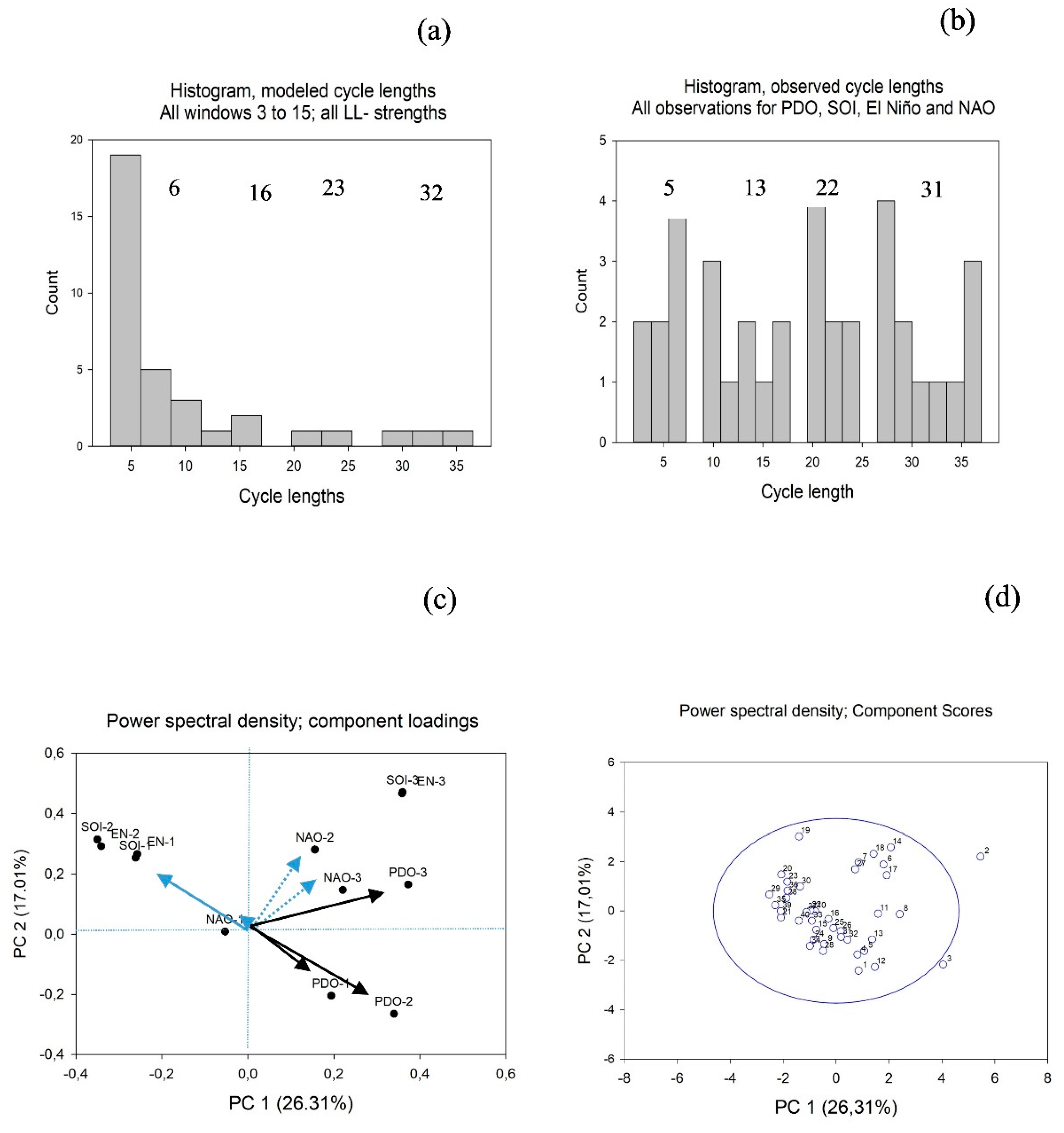
The time series are shown centered and normalized to unit standard deviation in Figure 1c. The figure shows both the raw series and series LOESS smoothed (window as fraction of full series f = 0.2 and a second order polynomial fitting). Figure 1a–b, d will be examined in the results section, but are included here to ease comparison of results with idealized sine function series.

In the present study, we used the random generators that are standard in Excel and in MatLab. They generate uniformly random numbers. However, it appears that random function generators may introduce periodic components [36]. Cycles of five steps long have a probability of occurring of less than 5% [35].

3. Methods

The method for identifying cycles and their lengths is described in Seip and Grøn [37]. We; therefore, here only give a short summary of two key features of the method that are used to develop the minimum model for cycle length. These are: (i) Identification of leading–lagging relations between two cyclic time series that impact each other, and (ii) the identification of common cycles for the paired series. The method is different from the ordinary cross correlation techniques (e.g., as applied to the Atlantic Meridional Overturning Circulation (AMOC) in Escudier et al. [1] or to PDO in Fleming [38]). The method does not require the series to be stationary, not even over a short interval. There have been other attempts to overcome requirements for long, stationary series [39], and a survey is given in Kestin et al. [27]. However, even with techniques that examine rolling time windows, window lengths are at least 10-, preferably 21-time-steps long. Furthermore, results may be distorted by additional methodical assumptions, like using frequencies that belong to a discrete harmonic set for windowed Fourier transforms [27]. A second type of method uses covariance estimates [20,40], and with increasing sample length the method gives more reliable results. The window length for the LL method is only used to establish confidence intervals by applying a Monte Carlo test to stochastic data. The LL method identifies common cycle lengths for the paired series, but there may still be other cycles superimposed on the series.

3.1. Quantifying Running Leading–Lagging Relation for Pairs of Variables

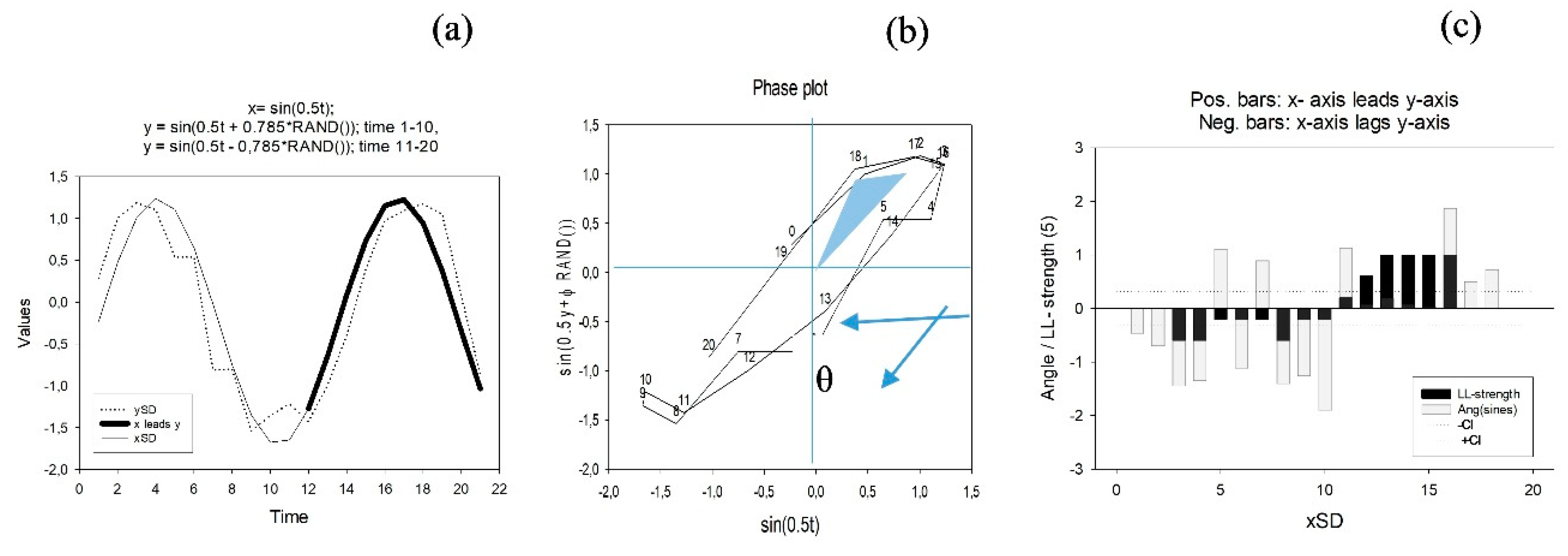
In the present work the leading–lagging (LL) method determines the LL relations for paired synoptic series of two times three observations. The LL method is explained with reference to Figure 2. At the basis of the method is the dual representation of paired cyclic time series, x (t) and y (t), in time representation and as phase plots. As time series the x-axis represents time and the x(t) and y(t) variables are plotted on the y-axis. As phase plot, the paired time series are depicted on the x-axis and the y-axis on a 2D graph, Figure 2b.

If one series leads another series with less than half a cycle length, then we will have persistent rotational direction of the series trajectories in the phase plot. Figure 2a,b give an example with x(t) = sin t and y(t) = sin (ωt + φ), φ = + 0.785 for time steps 1 to 9 and φ = –0.785 for time steps 10 to 20.

We explain the leading–lagging LL method in four steps.

Step 1. The data are linearly detrended.

Step 2. Rotational directions in phase space. The angle θ between two successive vectors ${\mathbf{V}}_1$ and ${\mathbf{V}}_2$ through three consecutive observations are calculated from:

$$\theta =sign(v_1\times v_2)\cdot \mathrm{Arccos}\left(\frac{v_1\cdot v_2}{\left|v_1\right|\left|v_2\right|}\right)$$

(1)

The rotational direction for the paired series in Figure 2a is shown as gray positive bars (counter clock-wise rotations) and as gray negative bars (clock-wise rotations) in Figure 2c.

Step 3. The LL strength of the mechanisms that cause two variables to either rotate clock-wise or counter clock-wise in a phase portrait is measured by the number of positive rotations (as sign(θ) > 0) minus the number of negative rotations (as sign(θ) < 0), relative to the total number of rotations over a certain period.

$$LL=\left(N_{pos}-N_{neg}\right)/\left(N_{pos}+N_{neg}\right)$$

(2)

This means that we can assess the persistence of the rotational direction. We use the nomenclature: LL (x, y) ∈ [−1,1] for leading–lagging strength: LL (x, y) < 0 implies that y leads x, y→x; LL (x, y) > 0 implies that x leads y, x→y. In a range around LL(x,y) = 0, no LL relations are significant.

Significance levels are calculated with Monte Carlo simulations for the LL strength measure. We found the 95% confidence interval for the mean value (zero per definition) to be ±0.32 for n = 9, that is, in a phase plot the series cycle persistently clock-wise or persistently counter clock-wise. This corresponds to significant leading–lagging signatures for the series shown in Figure 2c, black bars.

Step 4. The cycle length (CL) of two paired series that interact are approximated as:

$$CL=n\times 2\pi /\left({{\displaystyle \sum }}_2^{n-1}{\theta }_{i-1,i,i+1}\right)$$

(3)

where θ_i−1,i,i+1 is the angle between two consecutive vectors determined by three consecutive observations. The number of angles that close a full circle corresponds to the cycle length. With two perfect sines (no random component added and series normalized to unit standard deviation as in Figure 2b), we found CL = (λ) = 6.30, which is close to the design cycle length of λ = 2π ≈ 6.28. With a phase shift of λ/4, the trajectories form a closed circle and the average angle is −1.00 ± 0.00 radians. With a phase shift of λ/2, the average angle is −1.07 ± 0.48, that is, the rotational pattern is an ellipse. We get the same average angle, but with greater standard deviation. The wedges in Figure 2b suggest that the cycle time corresponds to the number of time steps, 1, 2, required to fill the ellipse with wedges.

3.2. The Minimal Statistical Model for Ocean Current Interactions

Our hypothesis is that if a pair of stochastic time series happens to show leading–lagging relations for n time steps, then that portion of the time series will also show a specific cycle length. We start with two time series 131 samples long and generated by uniform distributions. The series are hypothesized to represent annual observations of two ocean oscillations and are centered and normalized to unit standard deviation. We calculate the leading or lagging relations between the two series by using running time windows of lengths (WL) = 3, 5, 7, 15, and examine how many relations that by chance show persistent leading or lagging relations. That is, as we move downward the time series, i = 1–131, we examine the LL strength for the window i − n to i + n. With n = 1, we get 3 paired observations (WL = 3). If 3 of 3 paired observations show the same LL relation, then the LL strength = 1.0 and we calculate CL, for those cases from Equation (3). With n = 2, the window length is 5, and we examine if 5 of 5, 4 of 5, or 3 of 5 paired observations show the same LL relations (the LL strength is then 1.0, 0.8, 0.6 respectively), and we calculate the CL for those cases. This is repeated 10,000 times for window lengths 3 to 15. For a given window length, the percentage cycles of a certain length are thereafter divided by the total number of cycle lengths. We obtain a series of cycle lengths, which we can compare with the cycle lengths observed for ocean oscillations.

3.3. Power Spectral Density

The normal power spectral density (PSD) algorithm is applied to the full time series and to two subseries divided at 1950. The 3 PSD series are also normalized to unit standard deviation. We use a version of the multiple window spectrum method, [36] and stack PSDs both from the same series and from series that collectively will characterize the teleconnection system. Calculations are made in Excel, Matlab, and with SigmaPlot 14©. The full series do not have sufficient length to identify cycle lengths longer than the length of the time series, but we cautionary only allow half the time series length.

3.4. Principal Component Analysis (PCA)

Principal component analysis is a technique for extracting data from a complex matrix which relates several samples (normally presented as rows) of variables (columns) to define a few series (the principal components) that express the major information in the matrix data. PCA normally results in two plots. The loading plot shows how the variables relate to each other. Variables that are similar in a least square sense cluster together, whereas variables that are unrelated are perpendicular to each other when the variable symbols are connected to the origin with lines. However, for cyclic variables, the interpretation of the PCA plots will have another interpretation than for linear data with added stochastic noise. Figure 1a shows a set of sine functions that are shifted 1/16, 1/8, etc. of the cycle length relative to each other. Figure 1b shows the corresponding PCA loading plot. Sine functions that are shifted λ/4 relatively to each other will show a circle when plotted in a phase plot and; therefore, have a regression coefficient, r = 0. Paired time series that have regression coefficients of zero will appear in the phase plot at a right angle to each other, as in the loading plot in Figure 1b.

Significance levels for the PCA were identified by adding random numbers to the columns and the rows of the PCA matrix and then calculating 95% confidence intervals for the random numbers. Adding random numbers distorts the PCA algorithm to a certain degree, so the confidence estimates are only guiding values. However, confidence bands are difficult to obtain when PCA is applied to cyclic, non-normal data.

4. Results

We first provide a principal component analysis for the four raw ocean oscillation time series to get an impression of how the data relate to each other. Thereafter we apply power spectral analysis to the ocean oscillation data. Third, we present the results of the minimal model we hypothesize will give a basic explanation of the cycles observed in the ocean oscillations. Fourth, we compare model results to observations. Fifth, we examine the time series before and after 1950 and, finally, we report on the actual persistence of LL relations between the NAO–El Niño pair and the PDO–El Niño pair.

4.1. Relations between Four Ocean Oscillation Time Series

The PCA results for the four ocean oscillations in Figure 1d were compared to the loading plot for sine functions in Figure 1b. The SOI and El Niño (EN) were very similar, the PDO was almost half a cycle length, λ/2, out of phase with the SOI and El Niño, and the NAO was about λ/4 out of phase with the PDO, the SOI, and El Niño. The interaction relations will be treated in the discussion.

Since there was an improvement in the quality of the El Niño–Southern Oscillation observations around 1950, we divided the series into two subseries, one from the beginning of the observation period until 1949, and one from 1950 to the end of the observation period. A second reason for dividing the series was to examine if there were systematic changes in the PSD between the two time windows, caused either by increasing anthropogenic CO₂ emissions or by changes in the multidecadal ocean oscillation.

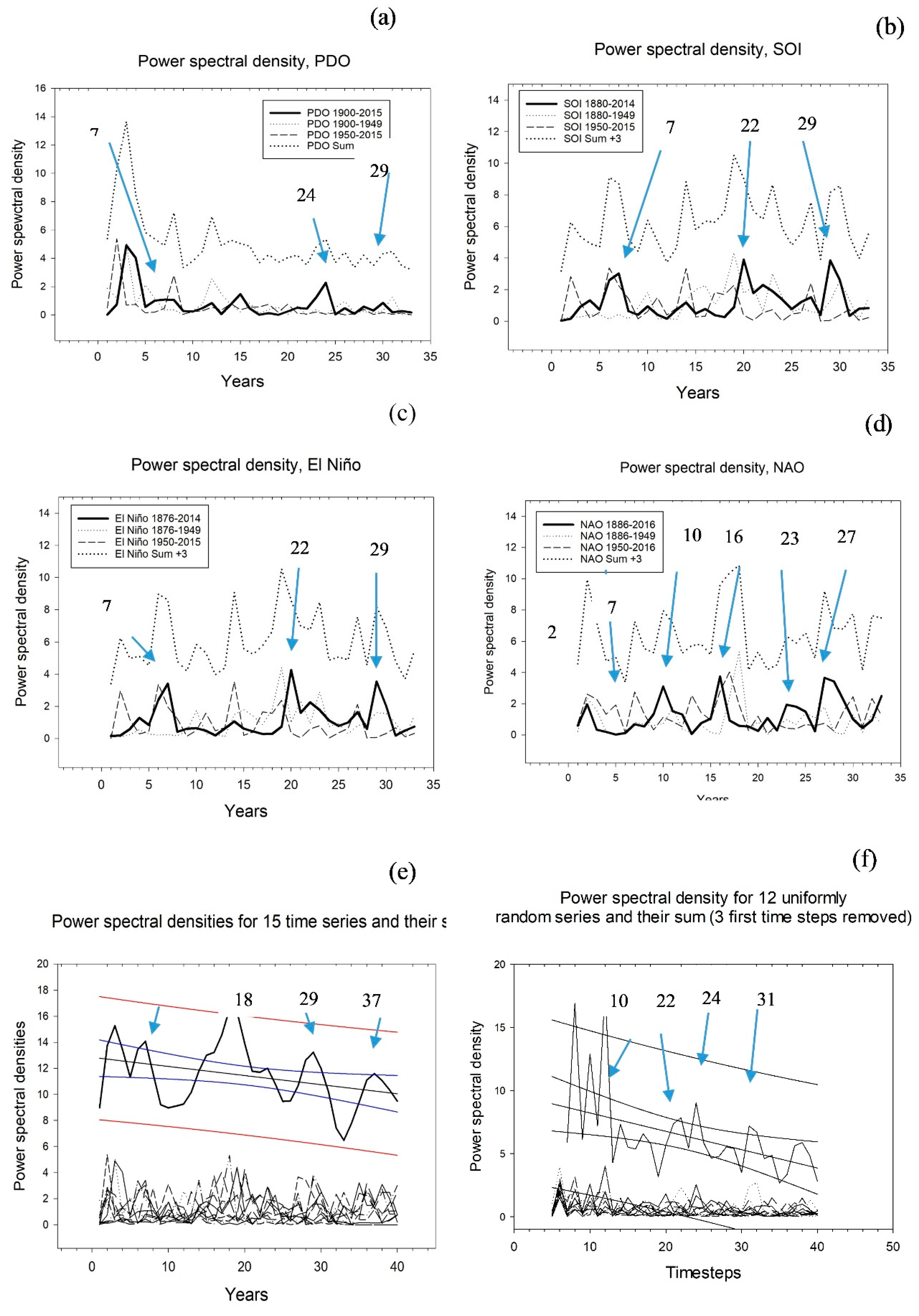
The power spectral densities (PSD) normalized to unit standard deviation and slightly LOESS smoothed f = 0.1, p = 2, are shown in Figure 3a–d. The PSD for the full series is outlined in bold. The uppermost curve in all four panels shows the sum of the three curves. The PSD for the full series dominated the pattern. The peaks in the PSD and the cycle lengths corresponding to the peaks are shown in

Table 1. Peaks in power spectral density curves. The full time series for the oscillations. “Sum” is all time series, including each of the sub periods before and after 1950. Numbers in bold designate peaks that visually higher than neighboring peaks.

Time Series	Peaks
PDO-1	3, 7, 12, 15, 21, 24, 29, 30, 35
SOI-1	4, 7, 10, 14, 16, 20, 22, 27, 29, 36
El Niño-1	4, 7, 10, 14, 20, 22, 27, 29, 36
NAO-1	2, 7, 10, 16, 21, 23, 27, 33, 37
Sum PDO, SOI, EN, NAO	3, 7, 18, 23, 29, 37
12 Uniform stochastic series	4, 6, 10, 22, 24, 31

. Cycle lengths that correspond to pronounced peaks, that is, peaks that are visually higher than neighboring peaks in the graphs, are marked in bold. Cycle lengths of seven years were pronounced for all four ocean oscillations. The power spectral densities are shown as tables in Supplementary Materials 1. In Supplementary Materials 2 the power density spectra for the raw series are shown graphically.

We hypothesize that by stacking the full series and sub-series on top of each other, cycle lengths that would dominate the ocean oscillation system would stand out, whereas other cycle lengths would cancel out. The result is shown in Figure 3e. For the stacked series, five peaks exceed the 95% confidence interval for the mean. Their corresponding cycle lengths are 3, 7, 18, 29, and 37 as shown in Table 1. We compared the PSD results for the stacked 12 ocean oscillations time series to 12 stacked PSD based on 12 uniformly stochastic series. As shown in Figure 3f, the stochastic distributions have peaks exceeding the 95% confidence band at 4, 6, 10, 22, 24, and 31 time steps.

4.2. Minimal Model Results

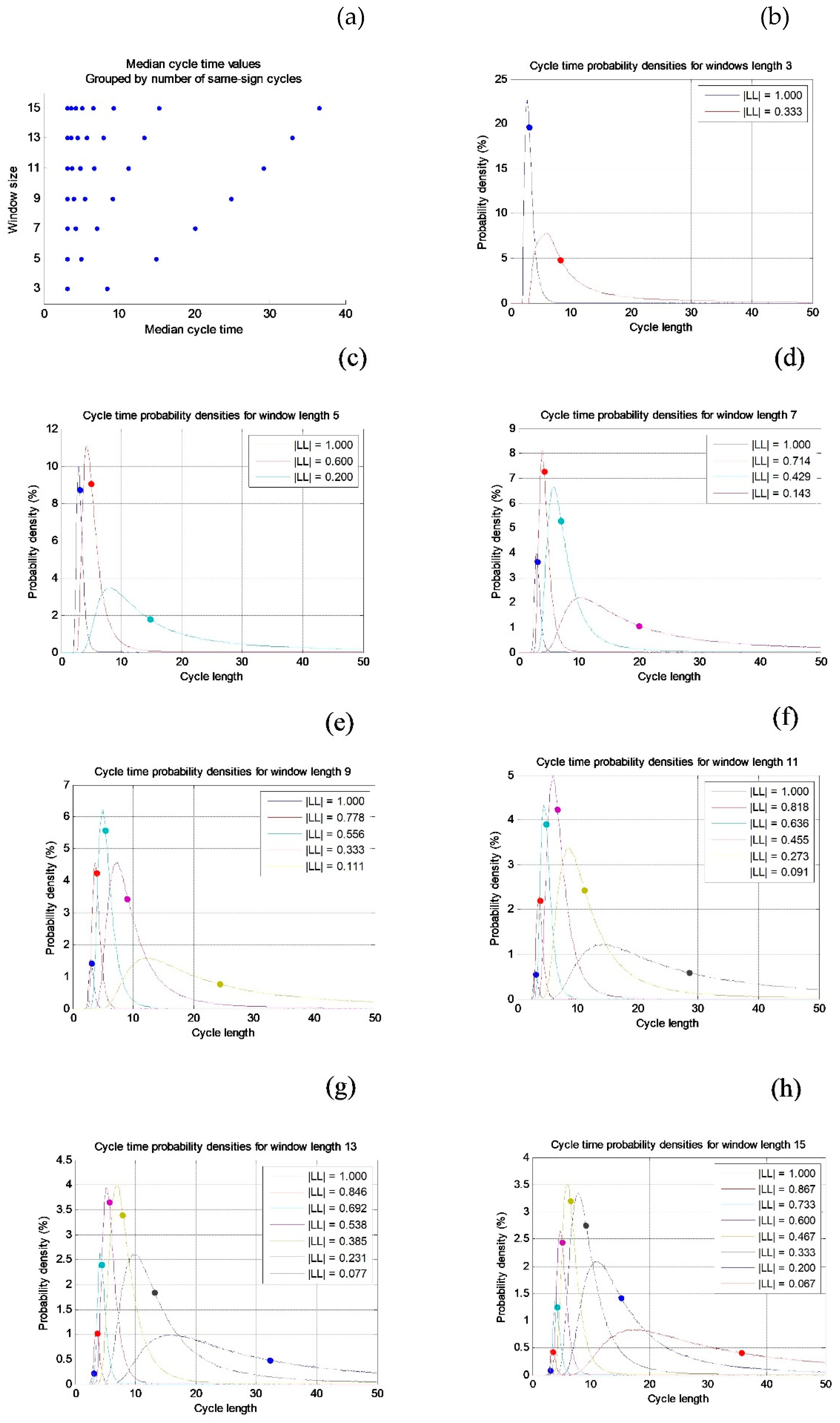
When one random series becomes a leading series to a second series, the two series show distinct cycles. We used moving time windows of three to 15 time steps and calculated cycle times when the paired series showed a persistent leading or lagging relation. Figure 4a shows median cycle lengths (x-axis) as window size (y-axis). For example, with window size 3, there can be a persistent LL relation for two or three time steps. The corresponding cycle lengths are 3.09 and 8.43 time steps. Numerical values corresponding to the graphs in Figure 4a are shown in Supplementary Material 3. Persistent LL sequences may create cycle lengths that are longer than the LL sequences. For example, sequences that are 15 years long may give distinct cycle lengths that are ≈30 years long. Figure 4b–h show the probability density function for cycles with increasing window sizes. A dot indicates the median value, which is to the right of the mode value (max value). The probability density functions have been normalized within each window length. With one million simulations, we found that the probability for 15 or more persistent leading or lagging relations in a sequence is less than 0.000215. To detect potential clustering of the cycle data, we calculated mean and standard deviation and constructed histograms for the cycle data. In the following, each time step is one year.

4.3. Comparing Model Results and Observations

The probability distribution functions at high cycle lengths show that the median (and also the average) values are far from the mode. When we compare the observed values with the results from the minimal model, the peaks shown in the PSD for the observed series, Figure 3, are sharper and more distinct than the probability density indicates for the model results, Figure 4. Therefore, we compared the peaks in the observed PSD shown in Figure 3 with the median values calculated in the model, Figure 4.

Histograms were made for the modeled distribution of cycle lengths across all time windows, 3 to 15, Figure 5a. We also made histograms for all four observed ocean oscillations combined, Figure 5b.

4.4. Comparing Time Series Cycles before and after 1950

One way to examine whether ocean oscillation observations are accurate before and after 1950 is to apply PSD to the sub-series before and after 1950. If the PSD are dissimilar, we would expect that the series are either sampled differently (the before-1950 sub-series probably sampled the most wrongly), or the development of the ocean oscillations is different before and after 1950. To examine similarities and differences between the PSD based on the full series and the sub-series before and after 1950, we constructed a matrix where the rows represent the cycle times: 1, 2, 3… to 40, and the columns show the ocean oscillations as 1 = full series, 2 = beginning–1949, 3 = 1950–end. The results are shown in Figure 5c,d. The PSDs for the El Niño series and the SOI series appear to overlap almost completely. However, there are differences between the sub-series and the full series for the NAO and the PDO.

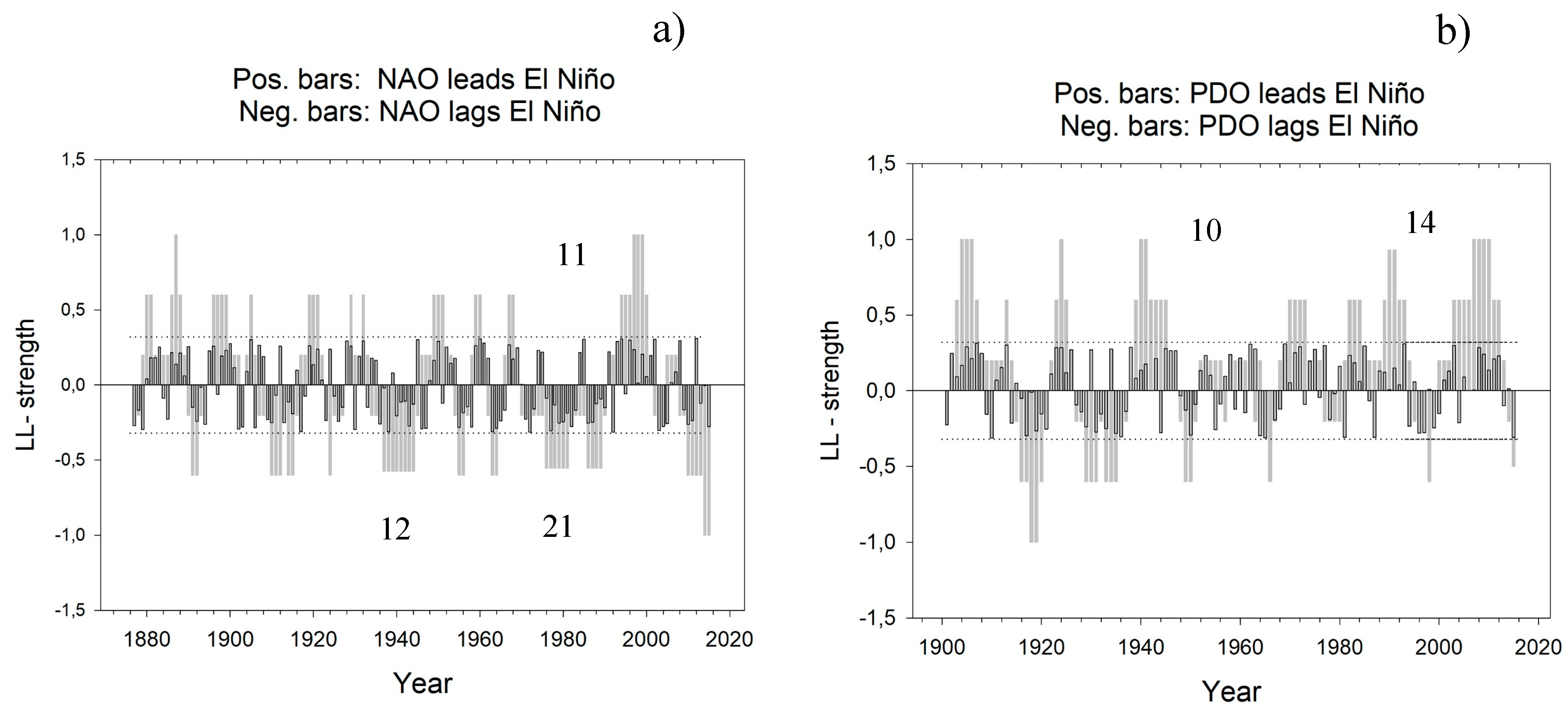
4.5. Observed LL Relations between the NAO and El Niño and the PDO and El Niño

We have calculated the actual number of times one ocean oscillation is a leading oscillation to another. Visually, the leading ocean oscillation consistently peaks less than a cycle length before the other. Running LL relations for the two pairs, NAO and El Niño and PDO and El Niño are shown in Figure 6a,b, respectively. The black bars show LL relations with n = 3, and the gray bars show average LL relations for five years, n = 5. (With LL = 1.0 or LL = −1, all 5 years have the same leading relation.) The dashed lines show 95% confidence limits for window lengths 9. The numbers in the graphs indicate windows where the LL relations persist for a long time. For the El Niño NAO pair, there are long persistent cycles that end in 1945, 1990, and 2001. For the PDO El Niño pair, there are long persistent cycles that end in 1947, 1994, and 2014.

The average number of persistent LL relations (not necessarily significant) is 6.6 years (both directions, range one to 21 years). For the NAO–El Niño pair, it is 4.2 years (range one to 11 years) when El Niño leads PDO and 8.4 years (range one to 14 years) when El Niño lags PDO. In Supplementary Material 4, the lengths of persistent LL relations are shown graphically. We then return back to Figure 1d to examine the relationship between the NAO–El Niño interaction, LL (NAO–El Niño), and the NAO index. From Figure 1d, it is seen that NAO leads El Niño when the NAO index is high. The relationship between LL (PDO, El Niño) and ocean oscillation time series is less pronounced.

5. Discussion

We first discuss the observed and modeled results and then compare the two. Last, we discuss the four theories for why distinct cycles occur.

5.1. Observations and Model Results Show Common Distinct Cycles

We first discuss the observed cycle estimates, then the modeled estimates, and, last, we compare the two estimates.

5.1.1. Observed Cycle Estimates

The PSD plots for the PDO, the SOI, El Niño, and the NAO gave common cycles at seven, 18, 29, and 37 years. The result is supported by our finding that the SOI and El Niño gave very similar results, in spite of characterizing different, but overlapping ocean regions, and in spite of being measured by temperature and sea level pressure, respectively. Additional support is given by the good correspondence between our cycle length estimates and the estimates for century-long time series of sea surface ice cover and sea level pressure in the Arctic by Venegas and Mysak [6]. They found four distinct cycle times of six to seven, nine to 10, 16 to 20 (centered at 18 years), and 30 to 50 years for “natural climate variability.” These authors also suggest atmospheric and morphological causes for the distinct cycle times (e.g., wind-driven motion of ice for the six- to seven-year cycle). Like us, they also examined if the improvement in data quality in 1950 changed their overall results. They concluded that a real regime shift around 1950–1960 could not be discarded.

We hypothesized that ocean basins that are separated (the North Atlantic Ocean and the Pacific Ocean) would interact less strongly than ocean basins that overlap (two basins in the Pacific Ocean). However, the average number of significantly persistent LL relations were 43%-47%, respectively, that is, with no appreciable differences. An interesting finding is also that the NAO index has a high value when it is a leading variable to El Niño.

5.1.2. The Model Estimate

We obtain better separation between cycle times with large window sizes time, that is, if oceanic oscillations show persistent leading relations for a long time (≈15 years, Figure 4a). Then cycle times above 30 years could be identified. Short cycle times are close, but in the model also distinct. Cycle times shorter than five years may occur with a probability greater than 5% in a uniformly random time series [35].

5.1.3. Comparing Observed and Modeled Distinct Cycles

The theory for distinct cycles presented in this paper explains several distinct cycles. The ultimate cause is the atmospheric and oceanic “bridges” that allow one ocean body to impact another ocean body so that their cycles are concerted for a prolonged time. Given a certain time window with concerted cycles, the cycle times are determined by properties of a uniform statistical distribution. The cycles are then observed as they give their fingerprint to temperature variations, sea-level pressure differences, or, as in the cases presented by Venegas and Mysak [6], as sea surface ice cover. Our results should be compared to results from modeling studies on teleconnections between ocean basins, like those of Roy et al. [42]. However, models like the CMIP5 still need improvement to adequately describe “bridges” between ocean basins [42].

5.2. Four Theories for Distinct Cycles

The sun–moon explanation focuses on the seven-year cycle. The TOA energy flux explanation shows cycle lengths that are three to four years long and thus within the range that could result from two stochastic series that impact each other. Still, the TOA explanation shows that the TOA energy flux is persistently and significantly leading the ocean heating rate for a period of 13 years (significance established for five running time windows, see Supplementary Materials 5). The ocean morphology explanation also shows periods in the range of three to five years, but such periods are also characteristic for oscillations in several ocean basins.

Our results extend the results in Seip and Grøn [17] in five ways. We include the NAO and the El Niño ocean oscillations, and second, we examine a continuum of window sizes. Third, we examine sub-series of the ocean oscillations before and after 1950. Fourth, we show that ocean interactions synchronize oscillation movements for two to above 20 years, but with a lag for one of the oscillations. Finally, we contrast our explanation of oceanic cycles to three alternative explanations in the literature.

6. Conclusions

We found evidence that the cyclic characteristics of ocean dynamics can be explained by a simple model that just depends upon the effect of one stochastic ocean oscillation exerting an impact on a second ocean oscillation so that movements in the two oscillations become concerted, but with a lag. Leading–lagging (LL) relations between ocean oscillations in different ocean basins prevail much longer than would occur by chance (<five years, a persistent series of 21 years has been observed). Thus, there must exist “bridges” that carry information from one basin to neighboring basins. The “bridges” and their strength are determined by atmospheric and ocean dynamics and there appear to be little distinction between basins that are separated and those that are overlapping. Since characteristic cycle lengths for oscillations before and after 1950 are different (their power spectral densities are different), we cannot exclude a regime shift in the climate around 1950.

As far as we can see, among the four theories that potentially could explain distinct cycles on a decadal- and multidecadal-scale, the theory that interactions between ocean basins give a leading relation between oscillations for a prolonged time is presently the only theory that explains the prevalence of several distinct cycles across oceans.